Samuel I . Outcalt, Kenneth M . Hinkel Erika Meyer, and Anthony J . Brazel

Application of Hurst Rescaling to Geophysical Serial Data

The empirical investigation of several geophysical time series indicates that they are composed of segments representing diferent natural regimes, or periods when events are strongly autocorrelated. Using a data transformation method devel- oped b y Hurst, these regimes are diferentiated b y rescaling the time series and examining the resulting transformed trace for inflections. As regime signals are not completely mixed and have rather long run lengths, Hurst rescaling pro- duces a clustering of extremes of the same sign and elevates the Hurst exponent to values greater than 0.5. These regimes have a characteristic distribution, as dejined b y the mean and standard deviation, which d i f e r f r o m the statistical characteristics of the complete record. Analysis of sunspot numbers, monthly precipitation records f r o m the midwestern United States, and annual watershed discharge yield regimes that correlate to well-documented periods of extreme activity. Rescaling appears to be useful in screening time series of unknown characteristics t o diferentiate periods dominated b y regime-specijic physical processes .

INTRODUCTION

The methods developed by Hurst (1951) to study the discharge of the Nile and other geophysical serial data are now recognized as pioneer explorations in natural fractal geometry (Mandelbrot 1982). Using historical records, Hurst was attempting to estimate the reservoir storage required to contain the Nile flood- water. To this end, he employed a technique of time-series transformation, referred to here as Hurst rescaling.

Hurst rescaling entails subtracting the mean of the series from each of the n observations in the record. These deviations from the mean are accumulated to

The senior author was first introduced to the fact that extremes in geophysical serial data are often temporally clustered by Professor Mark A. Melton during a graduate seminar at the Univer- sity of British Columbia in 1966; he never lost his interest in the problem. This research was par- tially supported by the National Science Foundation grants SES-9308334 and OPP-9529783 to KMH.

Samuel 1. Outcalt is adjunct professor emeritus, Kenneth M. Hinkel is associate pro- fessor, and Erika Meyer is a graduate student in the department of geography at the University of Cincinnati. Anthony 1. Brazel is professor of geography at Arizona State University.

Geographical Analysis, Vol. 29, No. 1 (January 1997) 0 1997 Ohio State University Press

S. I . Outcalt, K . M . Hinkel, E . Meyer, and A. J . Braze1 73

form a transformed series R. The adjusted range R(n) of the series is equal to

The adjusted range, divided by the standard deviation (S) of the record, yields the rescaled range. The rescaled range is expected to increase asymptotically with the square root of the number of record observations (n). The exponent H , with an anticipated value of 0.5, is termed the Hurst exponent (Schroeder 1991). These relationships are shown as equation (1).

(Rmax - &in).

The value of H is crudely calculated as the log of the rescaled range divided by the number of observations, as shown in equation (2).

H = log [R(n)/S(n)]/logn.

This form of equation (2) is used by Schroeder (1991, p. 130), and described as “a convenient measure of the persistence of a statistical phenomena.” It is employed here rather than the form favored by Potter (1979), in which the denominator is log (n ls ) .

Through empirical observation, Hurst and others recognized that, for many geophysical time series, the value of H is greater than 0.5 and frequently ranges from 0.6-0.9 (Hurst, Black, and Simaika 1965; Church 1980). This effect has been termed the Hurst phenomenon. Interpretations of the Hurst phenomenon have been abundant in the geophysical literature. Mandelbrot and Wallis (1969) and Mandelbrot (1982) attribute the nonrandom behavior of river discharge to “persistence,” which is the temporal grouping of nonperiodic, similar events. Furthermore, they associate Hurst exponent values with fractional noises. The Hurst exponent can range from brown noise ( H = 0.5) for a series with little persistence, through black noise ( H = 1.0) which characterizes extreme persis- tence. A value of H near 0.5 therefore indicates chaotic effects due to weak information storage capacity, and this is observed as an absence of long-term temporal correlations (Stolum 1996).

Klemes (1974), however, states that the heightened persistence of the Hurst phenomenon may be the result of a nonstationary, or shifting, record mean. He also claims that H values can be affected by characteristics of the stream storage system, and therefore asserts that a physical, rather than a mathematical, model of the effect would be extremely useful. Potter (1976, 1979), Church (1980), and Mesa and Poveda (1993) also attribute the Hurst phenomenon to a nonstation- ary mean. Conversely, Wallis and O’Connell (1973) suggest that the Hurst phe- nomenon can be explained with a mixed autoregressive-moving average model. Boes and Salas (1978) demonstrate that the nonstationary model is but a special case of the mixture model, as they have the same correlation structure and gen- erate similar pox diagrams. Thus, it is generally believed that elevated values of H result from pooling samples with different distribution characteristics.

This study will concentrate on the fundamental aspect used by Hurst and others-the rescaling transformation. In particular, we will demonstrate the power of Hurst rescaling in screening serial data for regime transitions. These occur at significant rescaled trace inflections, which signal the boundary of time- series segments characterized by statistical properties differing from the com- plete time series. The regimes that are defined by Hurst rescaling presumably reflect the effects of changes in the forcing mechanisms for a major duration. In the examination of geophysical serial data, investigators frequently use arbitrary time divisions, such as decades of mean annual values, to test for significant

74 1 Geographical Analysis

changes using statistical parameters. Hurst rescaling liberates investigators from using arbitrary periods or the informal method of “visual decomposition.”

To achieve our goal, a simple nonstationary model will be employed that appears to be validated by the empirical data. Our general model is similar to that of Potter (1976), who initially attributed the Hurst phenomenon to regimes with different statistical distributions but later ascribed to “acquisition artifacts” effects; in this case, the movement of the weather station or stream gaging site (Potter 1979).

A CONCEPTUAL MODEL OF THE HURST EFFECT

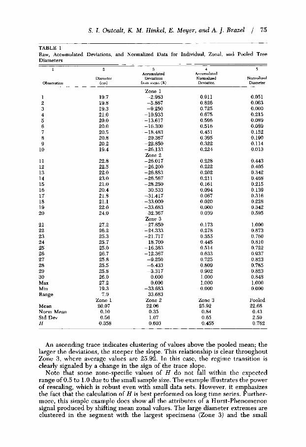
Suppose that one measured the diameters of trees found in three distinct zones along a transect. These zones could represent ecotones characterized by a differing dominant tree species, or could characterize regions in varying stages of vegetation succession. The diameter of each tree is recorded as a sequence by zone, as shown in Table 1. In this example, ten trees from each of the three zones yields a series of thirty observations. The maximum, minimum, mean, and standard deviation for each zone and the pooled sample are also reported.

Hurst rescaling entails accumulating deviations of the observation values from the pooled mean. For example, observation 1 has a circumference of 19.7 centimeters, which is 2.98 centimeters less than the pooled mean (22.68) as shown in the third column of Table 1. Observation 2 is 2.88 centimeters smaller than the pooled mean, and this deviation is added to the running sum to obtain -5.87.

Deviations from the pooled mean are thus calculated and accumulated for the entire series. Minimum and maximum deviations are used to calculate the adjusted range: in this case 33.683. As discussed earlier, the rescaled range is the adjusted range divided by the pooled standard deviation (33.683/2.586). Thus, from equation (2), H is 0.762 for the entire series, which suggests long- term persistence.

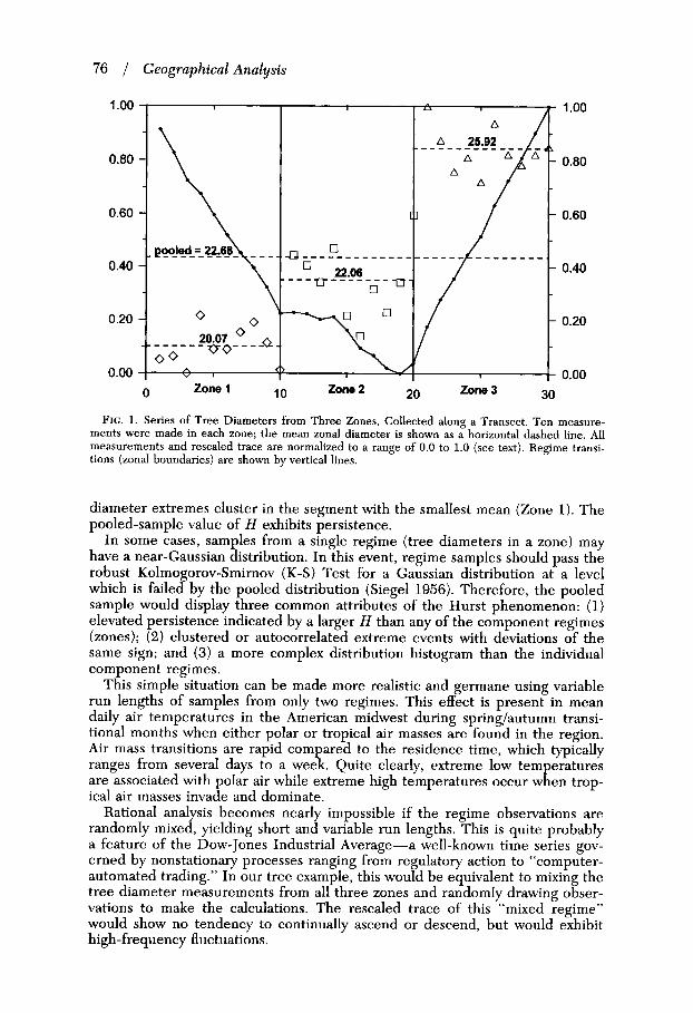
The advantage of rescaling is illustrated in Figure 1. Here, the observations are graphed as a series. In this and subsequent figures, all measurements and their transforms have been normalized to a range of 0.0 to 1.0. To normalize the tree diameters (column 5), for example, the minimum observed value of 19.3 is subtracted from each observation, and the remainder is divided by the sample range (7.9). In a similar manner, the rescaled sum in normalized by using the adjusted range of the rescaled series (-33.683), as shown in column 4. The sample and pooled means are calculated in the same way.

Normalization is performed for two purposes: (1) it allows the raw and re- scaled data to be displayed on the same diagram, and (2) normalization has no impact on the trace pattern or the estimate of H . For example, we could have first normalized the tree diameter data without affecting either H or the trace.

The primary advantage lies in the ease in interpreting the rescaled series. In Figure 1, it is clear that the Zone 1 average (20.07) is well below the pooled mean of 22.68. Thus, deviations are negative and accumulated deviations yield a trace with a negative slope for observations 1-10. A descending trace there- fore indicates persistence of lower-than-normal observations.

A significant trace inflection occurs near the zonal boundary at observation 10. Several of the Zone 2 trees have diameters approaching the pooled mean, yielding a trace with a slope near zero. Because most of the observations in Zone 2 are well below the pooled average, the overall slope is negative and the trace reaches a global normalized rescaled minimum value of 0.0 near the zonal boundary.

S . I . Outcalt, K . M . Hinkel, E . Meyer, and A. 1. Braze1 75

TABLE 1 Raw, Accumulated Deviations, and Normalized Data for Individual, Zonal, and Pooled Tree Diameters

1 2 3 4 5 Accumulated Accumulated

D i a m e t e r Deviations Normalized Normalized Observation (cm) from mean (R) Deviation Diameter

1 2 3 4 5 6 7 8 9

10

11 12 13 14 15 16 17 18 19 20

21 22 23 24 25 26 27 28 29 30 Max Min Range

Mean Norm Mean Std Dev H

19.7 19.8 19.3 21.0 20.0 20.0 20.5 20.8 20.2 19.4

22.8 22.5 22.0 23.0 21.0 20.4 21.8 21.1 22.0 24.0

27.2 26.2 25.3 25.7 25.0 26.7 25.8 25.5 25.8 26.0 27.2 19.3 7.9

Zone 1 20.07 0.10 0.56 0.358

Zone 1 -2.983 -5.867 -9.250

-10.933 -13.617 -16.300 -18.483 -20.367 -22.850 -26.133 Zone 2 -26.017 -26.200 -26.883 -26.567 -28.250 -30.533 -31.417 -33.000 -33.683 -32.367 Zone 3 -27.850 -24.333 -21.717 - 18.700 -16.383 -12.367 -9.250 -6.433 -3.317

0.000 0.000

-33.683 33.683

Zone 2 22.06 0.35 1.07 0.603

0.911 0.826 0.725 0.675 0.596 0.516 0.451 0.395 0.322 0.224

0.228 0.222 0.202 0.211 0.161 0.094 0.067 0.020 0.000 0.039

0.173 0.278 0.355 0.445 0.514 0.633 0.725 0.809 0.902 1.000 1.000 0.000

Zone 3 25.92 0.84 0.65 0.455

0.051 0.063 0.000 0.215 0.089 0.089 0.152 0.190 0.114 0.013

0.443 0.405 0.342 0.468 0.215 0.139 0.316 0.228 0.342 0.595

1.000 0.873 0.760 0.810 0.722 0.937 0.823 0.785 0.823 0.848 1.000 0.000

Pooled 22.68 0.43 2.59 0.762

An ascending trace indicates clustering of values above the pooled mean; the larger the deviations, the steeper the slope. This relationship is clear throughout Zone 3, where average values are 25.92. In this case, the regime transition is clearly signaled by a change in the sign of the trace slope.

Note that some zone-specific values of H do not fall within the expected range of 0.5 to 1.0 due to the small sample size. The example illustrates the power of resealing, which is robust even with small data sets. However, it emphasizes the fact that the calculation of H is best performed on long time series. Further- more, this simple example does show all the attributes of a Hurst-Phenomenon signal produced by shifting mean zonal values. The large diameter extremes are clustered in the segment with the largest specimens (Zone 3) and the small

76 f

1 .oo

0.80

0.60

0.40

0.20

0.00

1 .oo

0.80

0.60

0.40

0.20

0.00 30 Zone 3 20 Zone 2 10 Zone 1 0

FIG. 1. Series of Tree Diameters from Three Zones, Collected along a Transect. Ten measure- ments were made in each zone; the mean zonal diameter is shown as a horizontal dashed line. All measurements and rescaled trace are normalized to a range of 0.0 to 1.0 (see text). Regime transi- tions (zonal boundaries) are shown by vertical lines.

diameter extremes cluster in the segment with the smallest mean (Zone 1). The pooled-sample value of H exhibits persistence.

In some cases, samples from a single regime (tree diameters in a zone) may have a near-Gaussian distribution. In this event, regime samples should pass the robust Kolmogorov-Smirnov (K-S) Test for a Gaussian distribution at a level which is failed by the pooled distribution (Siege1 1956). Therefore, the pooled sample would display three common attributes of the Hurst phenomenon: (1) elevated persistence indicated by a larger H than any of the component regimes (zones); ( 2 ) clustered or autocorrelated extreme events with deviations of the same sign; and (3) a more complex distribution histogram than the individual component regimes.

This simple situation can be made more realistic and germane using variable run lengths of samples from only two regimes. This effect is present in mean daily air temperatures in the American midwest during springfautumn transi- tional months when either polar or tropical air masses are found in the region. Air mass transitions are rapid compared to the residence time, which typically ranges from several days to a week. Quite clearly, extreme low temperatures are associated with polar air while extreme high temperatures occur when trop- ical air masses invade and dominate.

Rational analysis becomes nearly impossible if the regime observations are randomly mixed, yielding short and variable run lengths. This is quite probably a feature of the Dow-Jones Industrial Average-a well-known time series gov- erned by nonstationary processes ranging from regulatory action to “computer- automated trading.” In our tree example, this would be equivalent to mixing the tree diameter measurements from al! three zones and randomly drawing obser- vations to make the calculations. The rescaled trace of this “mixed regime” would show no tendency to continually ascend or descend, but would exhibit high-frequency fluctuations.

S . 1. Outcalt, K . M . Hinkel, E . Meyer, and A. J . Braze1 / 77

200

150 m 0 Q

c 3

-cJ

100

50 v,

0 1500 1550 1600 1650 1700 1750 1800 1850 1900 1950 2(

Year

- U 0

0 2 - -

0 0 , ' 1 ' l ' 1 ' 1 ' 1 ' 1 ' 1 ' 1 ' 1 ' 1500 1550 1600 1650 1700 1750 1800 1850 1900 1950 21

Year

30

00

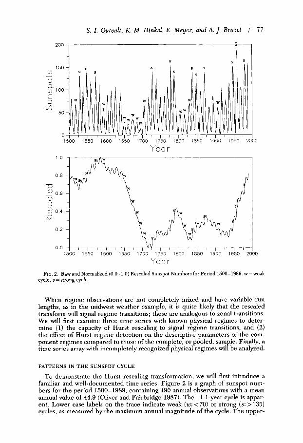
FIG. 2. Raw and Normalized (0.0-1.0) Rescaled Sunspot Numbers for Period 1500-1989. w=weak cycle, s =strong cycle.

When regime observations are not completely mixed and have variable run lengths, as in the midwest weather example, it is quite likely that the rescaled transform will signal regime transitions; these are analogous to zonal transitions. We will first examine three time series with known physical regimes to deter- mine (1) the capacity of Hurst rescaling to signal regime transitions, and (2) the effect of Hurst regime detection on the descriptive parameters of the com- ponent regimes compared to those of the complete, or pooled, sample. Finally, a time series array with incompletely recognized physical regimes will be analyzed.

PATTERNS IN THE SUNSPOT CYCLE

To demonstrate the Hurst rescaling transformation, we will first introduce a familiar and well-documented time series. Figure 2 is a graph of sunspot num- bers for the period 1500-1989, containing 490 annual observations with a mean annual value of 44.9 (Oliver and Fairbridge 1987). The 11.1-year cycle is appar- ent. Lower case labels on the trace indicate weak (w: <70) or strong (s: >135) cycles, as measured by the maximum annual magnitude of the cycle. The upper-

78 f Geographical Analysis

case labels indicate global extremes in the data set, with the weakest cycle peak magnitude occurring in 1694 (W = 20) and strongest in 1957 (S = 194).

The normalized rescaled time series is shown below and utilizes the same sym- bols. The general patterns are easy to interpret. To reiterate, an ascending trace occurs when a sequence of individual observations in the time series exceed the mean of the record, and these positive deviations are accumulated. A steep positive slope therefore indicates persistence of significantly higher-than-average values. Conversely, a trace descension results from the accumulation of obser- vations below the record mean, and a slope near zero denotes near-average con- ditions over the duration. Finally, regime transitions are often signaled by a change in the sign of the trace slope.

Several patterns are apparent in the normalized rescaled sunspot number trace. First, we note that high-frequency trace fluctuations are related to the sunspot cycle, and this subcyclic information is preserved. Second, we note a slight depression in the trace centered around 1525, which corresponds to the end of the Sporer minimum (1420-1530). Following this local minimum, the trace reaches a global maximum around 1580, produced by the cumulative im- pact of several recurring strong cycles.

The next 150 years show a decreasing trend toward a global minimum around 1715 caused by repeating weak cycles, including the weakest cycle in 1694 (W). This is the Maunder minimum, typically dated from 1645-1715. Note, however, the duration over which the trace is declining is greater by a factor of two. Since a declining trace occurs when recurring values less than the mean of the data set are summed, the negative slope suggests a gradual reduction in sunspot activity preceding the Maunder minimum as traditionally defined, and a period of recovery extending slightly beyond the observed global minimum in 1694 (W).

The 1700s are characterized by renewed sunspot activity, with several strong cycles. This pattern is reflected as an ascension of the normalized rescaled trace which peaks locally around 1778. Three weak solar cycles in the early 1800s are followed by three strong cycles clustered in the mid-1800s. The rapid ascension near the end of the record is due to clustering of strong cycles and includes the record maximum of 1957 (S).

The calculated Hurst exponent is 0.668 for the 490-year record. If the data are first detrended, H remains the same but the rescaled trace is modified. The overall pattern is the same, with inflection points occurring at the same time. However, the trace is progressively displaced downward with time since the linear trend was positive. Thus, the global minimum on the trace occurs during the first half of the twentieth century. Since the observed trend may well be part of a longer cycle [for example, two hundred years (Schove 1983)], it is a significant part of the signal and is not removed from the data (Bhattacharya, Gupta, and Waymire 1983).

PRECIPITATION RECORDS AND DROUGHT

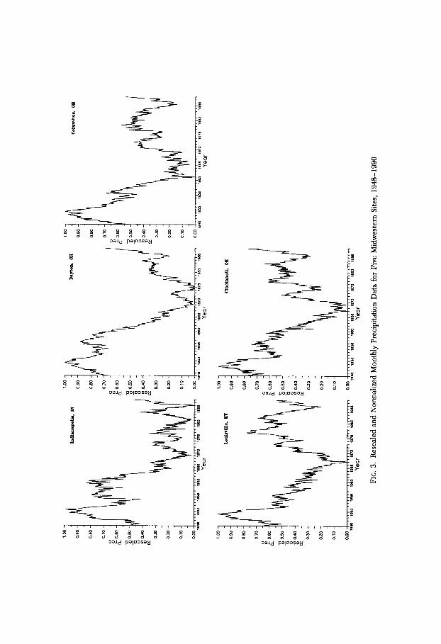
Potter (1976, 1979) used annual precipitation time series to identify nonsta- tionarity in the record. In his studies, one hundred years of data for sites in the northeastern United States were analyzed to detect precipitation regimes and to calculate the Hurst exponent. In a similar vein, monthly precipitation amounts for the period 1948 through 1990 were obtained for five NOAA meteorological stations in the midwestern United States (NOAA 1992). This yielded 516 obser- vations for forty-three years at each station, and includes some periods of signif- icant drought. The normalized rescaled time series are presented as Figure 3.

80 / Geographical Analysis

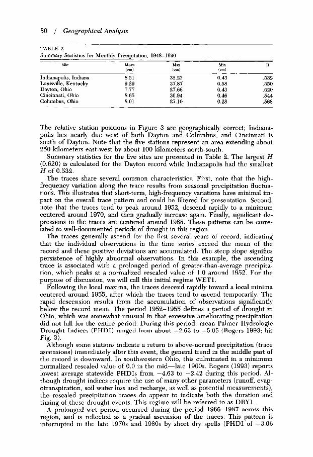
TABLE 2 Summary Statistics for Monthly Precipitation, 1948-1990

Site Mean M a Min H (cm) (cm) (cm)

Indianapolis, Indiana 8.51 32.23 0.43 ,532 Louisville, Kentucky 9.29 37.87 0.58 ,550 Dayton, Ohio 7.77 27.66 0.43 ,620 Cincinnati, Ohio 8.65 30.94 0.46 ,544 Columbus, Ohio 8.01 27.10 0.28 .568

The relative station positions in Figure 3 are geographically correct; Indiana- polis lies nearly due west of both Dayton and Columbus, and Cincinnati is south of Dayton. Note that the five stations represent an area extending about 250 kilometers east-west by about 100 kilometers north-south.

Summary statistics for the five sites are presented in Table 2. The largest H (0.620) is calculated for the Dayton record while Indianapolis had the smallest H of 0.532.

The traces share several common characteristics. First, note that the high- frequency variation along the trace results from seasonal precipitation fluctua- tions. This illustrates that short-term, high-frequency variations have minimal im- pact on the overall trace pattern and could be filtered for presentation. Second, note that the traces tend to peak around 1952, descend rapidly to a minimum centered around 1970, and then gradually increase again. Finally, significant de- pressions in the traces are centered around 1988. These patterns can be corre- lated to well-documented periods of drought in this region.

The traces generally ascend for the first several years of record, indicating that the individual observations in the time series exceed the mean of the record and these positive deviations are accumulated. The steep slope signifies persistence of highly abnormal observations. In this example, the ascending trace is associated with a prolonged period of greater-than-average precipita- tion, which peaks at a normalized rescaled value of 1.0 around 1952. For the purpose of discussion, we will call this initial regime WET1.

Following the local maxima, the traces descend rapidly toward a local minima centered around 1955, after which the traces tend to ascend temporarily. The rapid descension results from the accumulation of observations significantly below the record mean. The period 1952-1955 defines a period of drought in Ohio, which was somewhat unusual in that excessive ameliorating precipitation did not fall for the entire period. During this period, mean Palmer Hydrologic Drought Indices (PHDI) ranged from about -2.63 to -5.05 (Rogers 1993; his Fig. 3).

Although some stations indicate a return to above-normal precipitation (trace ascensions) immediately after this event, the general trend in the middle part of the record is downward. In southwestern Ohio, this culminated in a minimum normalized rescaled value of 0.0 in the mid-late 1960s. Rogers (1993) reports lowest average statewide PHDIs from -4.63 to -2.42 during this period. Al- though drought indices require the use of many other parameters (runoff, evap- otranspiration, soil water loss and recharge, as well as potential measurements), the rescaled precipitation traces do appear to indicate both the duration and timing of these drought events. This regime will be referred to as DRY1.

A prolonged wet period occurred during the period 1966-1987 across this region, and is reflected as a gradual ascension of the traces. This pattern is interrupted in the late 1970s and 1980s by short dry spells (PHDI of -3.06

S . I . Outcalt, K . M . Hinkel, E . Meyer, and A. J. Braze1 81

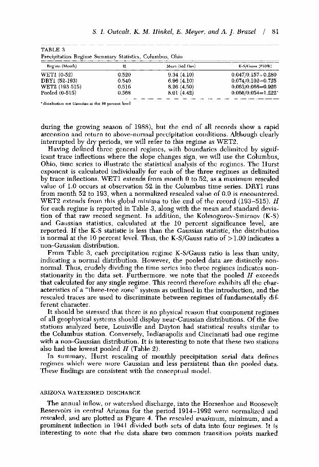
TABLE 3 Precipitation Regime Summary Statistics, Columbus, Ohio

Regime (Month) n Mean (Std Dev) K-S/Gauss (PIOJ)

WETl (0-52) 0.520 9.34 (4.10) 0.047/0.157=0.280 DRYl (52-193) 0.540 6.96 (4.10) 0.074/0.102=0.725 WET2 (193-515) 0.516 8.26 (4.50) 0.063/0.068=0.926 Pooled (0-515) 0.568 8.01 (4.42) 0.066/0.054=1.222*

‘distribution not Gaussian at the 10 percent level

during the growing season of 1988), but the end of all records show a rapid ascension and return to above-normal precipitation conditions. Although clearly interrupted by dry periods, we will refer to this regime as WETS.

Having defined three general regimes, with boundaries delimited by signif- icant trace inflections where the slope changes sign, we will use the Columbus, Ohio, time series to illustrate the statistical analysis of the regimes. The Hurst exponent is calculated individually for each of the three regimes as delimited by trace inflections. WETl extends from month 0 to 52, as a maximum rescaled value of 1.0 occurs at observation 52 in the Columbus time series. DRYl runs from month 52 to 193, when a normalized rescaled value of 0.0 is encountered. WET2 extends from this global minima to the end of the record (193-515). H for each regime is reported in Table 3, along with the mean and standard devia- tion of that raw record segment. In addition, the Kolmogorov-Smirnov (K-S) and Gaussian statistics, calculated at the 10 percent significance level, are reported. If the K-S statistic is less than the Gaussian statistic, the distribution is normal at the 10 percent level. Thus, the K-S/Gauss ratio of > 1.00 indicates a non-Gaussian distribution.

From Table 3, each precipitation regime K-S/Gauss ratio is less than unity, indicating a normal distribution. However, the pooled data are distinctly non- normal. Thus, crudely dividing the time series into three regimes indicates non- stationarity in the data set. Furthermore, we note that the pooled H exceeds that calculated for any single regime. This record therefore exhibits all the char- acteristics of a “three-tree zone” system as outlined in the introduction, and the rescaled traces are used to discriminate between regimes of fundamentally dif- ferent character.

I t should be stressed that there is no physical reason that component regimes of all geophysical systems should display near-Gaussian distributions. Of the five stations analyzed here, Louisville and Dayton had statistical results similar to the Columbus station. Conversely, Indianapolis and Cincinnati had one regime with a non-Gaussian distribution. It is interesting to note that these two stations also had the lowest pooled H (Table 2).

In summary, Hurst rescaling of monthly precipitation serial data defines regimes which were more Gaussian and less persistent than the pooled data. These findings are consistent with the conceptual model.

ARIZONA WATERSHED DISCHARGE

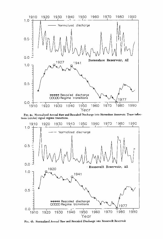
The annual inflow, or watershed discharge, into the Horseshoe and Roosevelt Reservoirs in central Arizona for the period 1914-1992 were normalized and rescaled, and are plotted as Figure 4. The rescaled maximum, minimum, and a prominent inflection in 1941 divided both sets of data into four regimes. It is interesting to note that the data share two common transition points marked

1910 1920 1930 1940 1950 1960 1970 1980 1990 1 .o

0.5

0.0

1 .o Horseshoe Reservoir, AZ

0.5

caled discharge ime transitions

0.0 1910 1920 1930 1940 1950 1960 1970 1980 1990

FIG. 4a. Normalized Annual Raw and Rescaled Discharge into Horseshoe Reservoir. Trace inflec- Year

tions (circles) signal regime transitions.

1 1 .o

0.5

0.0 Roosevelt Reservoir, AZ 1920

1.0 7 - - - - -

0.5 y - - - -

4++W Rescaled discharge Oxco Regime transitions -

0.0 I I I I I I U I I 1910 1920 1930 1940 1950 1960 1970 1980 1990

Year FIG. 4b. Normalized Annual Raw and Rescaled Discharge into Roosevelt Reservoir

S . I. Outcalt, K . M . Hinkel, E . Meyer, and A. 1. Brazel J 83

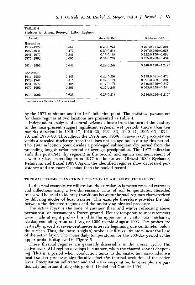
TABLE 4 Statistics for Annual Reservoir Inflow Regimes

Record H Mean (Std Dev) K-S/Gauss (P20%)

Horseshoe 1914-1927 0.567 1927-1941 0.472 194 1-1977 0.541 1977-1992 0.605

0.46(0.24) 0.107/0.274=0.391 0.29(0.21) 0.167/0.266=0.628 0.19(0.18) 0.122/0.176=0.693 0.34(0.28) 0.125/0.258=0.484

~ ~~ ~

1914-1992 0.640

Roosevelt 1914-1920 0.449 1920- 194 1 0.515 1941-1977 0.498 1977-1992 0.561

0.28(0.24) 0.146/0.120=1.217*

0.44(0.29) 0.179/0.381=0.470 0.22(0.17) 0.091/0.233=0.391 0.17(0.17) 0.149/0.176=0.847 0.33(0.24) 0.063/0.258=0.244

1914-1992 0.636 0.23(0.21) 0.146/0.120=1.217*

' distribution not Gaussian at 20 percent level

by the 1977 minimum and the 1941 inflection point. The statistical parameters for these regimes at two locations are presented as Table 4.

Independent analyses of central Arizona climate from the turn of the century to the near-present suggest significant regional wet periods (more than ten months duration) in 1915-17, 1919-20, 1931-33, 1940-41, 1965-66, 1972- 73, and 1978-80. Throughout the 1920s and 1930s, near-average precipitation yields a rescaled discharge trace that does not change much during this period. The 1941 inflection point divides a prolonged subsequent dry period from the preceding long-duration period of average precipitation. The 1977 inflection ends this post-1941 dry segment in the record, and signals commencement of a wetter phase extending from 1977 to the present (Brazel 1986; Eychaner, Rehmann, and Brazel 1989). Again, the identified regimes show decreased per- sistence and are more Gaussian than the pooled record.

THERMAL REGIME TRANSITION DETECTION IN SOIL ABOVE PERMAFROST

In this final example, we will explore the correlation between rescaled extremes and inflections using a two-dimensional array of soil temperatures. Rescaled traces will be used to identify transitions between thermal regimes characterized by differing modes of heat transfer. This example therefore provides the link between the detected regimes and the underlyng physical processes.

The active layer is the zone of summer thaw and winter refreezing above permafrost, or permanently frozen ground. Hourly temperature measurements were made at eight probes buried in the upper soil at a site near Fairbanks, Alaska, extending from mid-August 1992 to mid-August 1993. The probes are vertically spaced at seven-centimeter intervals beginning one centimeter below the surface. Thus, the lowest (eighth) probe is at fifty centimeters, near the base of the active layer. The mean daily temperatures for the 363-day period at the upper probe is displayed in Figure 5.

Three thermal regimes are generally discernible in the annual cycle. The active layer (AL) regime develops in summer, when the thawed zone is deepen- ing. This is a period when conduction tends to dominate, but nonconductive heat transfer processes significantly affect the thermal evolution of the active layer. Precipitation infiltration and soil water evaporation, for example, are par- ticularly important during this period (Hinkel and Outcalt 1994).

84 / Geographical Analysis

0 30 60 90 120 150 180 210 240 270 300 330 3

-2 O 4 I

1 6 - 14-

-12- 0

8 - a -

4 -

- Upper (1 -cm) probe

,lo:

t-

-2 i

-41 I

0.2

0.4 1

Upper (1 -cm) probe

~

Rescaled

ZC-FR

.. 0.0 I I I I I I I I I I I I 0 30 60 90 120 150 180 210 240 270 300 330 31

Day Index FIG. 5. Mean Daily and Rescaled Temperature from Near-Surface Probe for Period Mid-August

1992 to Mid-August 1993. AL = active layer regime; ZC =zero curtain regime; FR =freezing regime.

As the active layer refreezes from the surface downward in autumn and early winter, temperatures in the lower part of the active layer are isothermal near O'C, often for several months. This is known as the zero-curtain efect (Sumgin et al. 1940), and this period is referred to as the zero curtain (ZC) regime. Although heat conduction cannot occur across an isothermal zone, water and water vapor migrate vertically across the unfrozen layer in response to osmotic gradients, transporting both sensible and latent heat upward. This regime is therefore dominated by nonconductive heat transfer effects (Outcalt, Nelson, and Hinkel 1990).

In mid-late winter, as subfreezing temperatures penetrate to depth, the active layer freezes and the freezing (FR) regime commences. Once the path- ways between soil pores become blocked with ice, the movement of water and water vapor is restricted and conduction dominates. This regime is truncated with spring thaw and the AL regime begins the cycle again.

These divisions are based on the dominant heat transfer process, so the regime patterns are known from other analyses (Outcalt, Nelson, and Hinkel 1990; Hinkel and Outcalt 1994, 1995). Regime transitions, however, are not easily discriminated. The statistics for the three regimes identified by rescaling are reported in Table 5.

S . I . Outcalt, K . M . Hinkel, E . Meyer, and A. J . Braze1 85

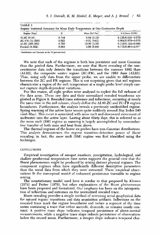
TABLE 5 Regime Statistical Summary for Mean Daily Temperature at One-Centimeter Depth

Regime (Days) H Mean (Std Dev) K-S/Gauss (PIOB)

AL92 (0-31) 0.744 6.84 (3.16) 0.125/0.216=0.579 ZC-FR (31-266) 0.823 -0.81 (0.61) 0.064/0.079=0.8 10 AL93 (266-362) 0.760 10.80 (3.50) 0.119/0.124=0.960 Pooled (0-362) 0.863 2.96 (5.60) 0.172/0.064=2.87*

‘distribution not Gaussian at the 10 percent level

We note that each of the regimes is both less persistent and more Gaussian than the pooled data. Furthermore, we note that Hurst rescaling of the one- centimeter data only detects the transitions between the summer 1992 thaw (AL92), the composite winter regime (ZC-FR), and the 1993 thaw (AL93). Thus, using only data from the upper probe, we are unable to differentiate between the ZC and FR regimes. This is not surprising given that soil regimes characterize a region of the soil; temperature at a single probe level simply can- not capture depth-dependent variations.

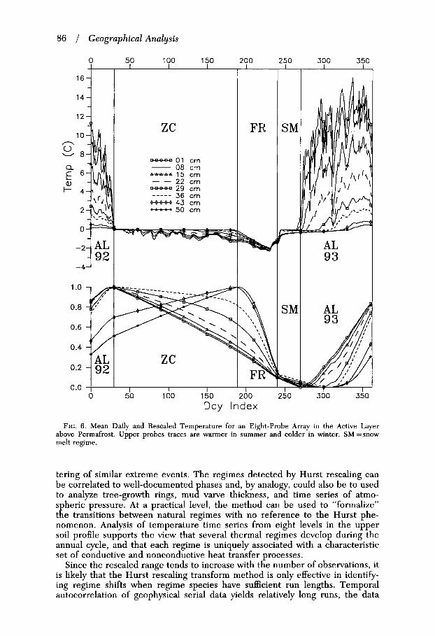
For this reason, all eight probes were analyzed to exploit the full richness of the data array. These raw data and their normalized rescaled transforms are plotted as Figure 6. Rescaled trace extremes and inflections, occurring at nearly the same time in the soil column, clearly define the AL92-ZC and ZC-FR regime boundaries. Furthermore, the analysis reveals a previously unidentified regime. Spring warming of the active layer occurs quite suddenly around Day Index 240 (mid-May). This event is associated with snow melt and downward movement of meltwater into the active layer. Lasting about thirty days, this is referred to as the snow melt (SM) regime as warming is largely accomplished by nonconduc- tive transfer of both mass and heat from above.

The thermal regimes of the lower six probes have non-Gaussian distributions. This analysis demonstrates the regime transition-detection power of H u n t resealing; in fact, the snow melt (SM) regime was first identified using the technique.

CONCLUSIONS

Empirical investigation of sunspot numbers, precipitation, hydrological, and shallow geothermal temperature time series supports the general view that the Hurst phenomenon might be produced by mixing distinct physical regimes. The component regimes often have significantly different descriptive parameters than the serial data from which they were extracted. These empirical obser- vations fit the conceptual model of enhanced persistence traceable to regime mixing.

The nonstationary model used here is similar to that proposed by Klemes (1974) and Potter (1976), but other explanations of the Hurst phenomenon have been proposed and formalized. Our emphasis has been on the interpreta- tion of inflections and extremes on the normalized rescaled trace.

Hurst rescaling provides a simple method of screening serial geophysical data for natural regime transitions and data acquisition artifacts. Inflections on the rescaled trace mark the regime boundaries and isolate a segment of the time series containing a trace that either ascends, descends, or remains nearly con- stant. A positive trace slope indicates temporal persistence of above-normal measurements, while a negative trace slope reflects persistence of observations below the record mean. Furthermore, a steeper slope indicates temporal clus-

86 / Geographical Analysis

0

1 .o

0.4

0.2

0.0 0

50 100 150 200 250

zc

-01 c m - 08 c m -15 crn

22 cm -29 cm

36 c m w+ew 43 cm - 5 0 cm

- - _-___

FR S M

S M

50 100 150 200 250 Day Index

300 350

AL 93

300 350

FIG. 6. Mean Daily and Rescaled Temperature for an Eight-Probe Array in the Active Layer above Permafrost. Upper probes traces are warmer in summer and colder in winter. SM =snow melt regime.

tering of similar extreme events. The regimes detected by Hurst rescaling can be correlated to well-documented phases and, by analogy, could also be to used to analyze tree-growth rings, mud varve thickness, and time series of atmo- spheric pressure. At a practical level, the method can be used to “formalize” the transitions between natural regimes with no reference to the Hurst phe- nomenon. Analysis of temperature time series from eight levels in the upper soil profile supports the view that several thermal regimes develop during the annual cycle, and that each regime is uniquely associated with a characteristic set of conductive and nonconductive heat transfer processes.

Since the rescaled range tends to increase with the number of observations, it is likely that the Hurst rescaling transform method is only effective in identify- ing regime shifts when regime species have sufficient run lengths. Temporal autocorrelation of geophysical serial data yields relatively long runs, the data

S . I . Outcalt, K . M . Hinkel, E . Meyer, and A. 1. Brazel 1 87

attribute that makes regime transitions detectable at a site. Complete regime mixing is not probable in climate-governed geophysical time series as the global fluid systems have strong persistence. This nearly universal species persistence is an attribute of geophysical systems that makes regime identification tractable at a site. This is a general attribute of hydro-climatological serial data that is forced, to a large extent, by circulation pattern transitions in the large fluid sys- tems of the atmosphere and oceans.

LITERATURE CITED

Bhattacharya, R. N., V. K. Gupta, and E. Waymire (1983). “The Hunt Effect under Trends.”Journal of Applied Probability 20, 649-62.

Boes, D. C., and J. D. Salas (1978). “Nonstationarity of the Mean and the Hunt Phenomenon.” Water Resources Research 14( l) , 135-43.

Brazel, A. J, (1986). “Statewide Temperature and Moisture Trends, 1895-1983.” In Arizona Climate: The First Hundred Years, edited by W. D. Sellers, R. H. Hill, and M. Sanderson-Rae, pp. 79-84. Tuscon: University of Arizona Press.

Church, M. (1980). “Records of Recent Geomorphological Events.” In Timescales in Geomorphology, edited by R. A. Cullingform, D. A. Davidson, and J. Lewin, pp. 13-29. New York: John Wiley and Sons.

Eychaner, J. H., M. R. Rehmann, and A. J. Brazel (1989). “Arizona Floods and Droughts.” Floods and Droughts, State Summaries. National Water Summary, 1988-89. USGS Water Supply Paper 2375, pp. 181-88.

Hinkel, K. M., and S. I. Outcalt (1994). “Identification of Heat Transfer Processes during Soil Cooling, Freezing, and Thaw in Central Alaska.” Permafrost and Perigkial Processes 5(4), 217-35.

(1995). “The Detection of Heat-Mass Transfer Regime Transitions in the Active Layer Using Fractal Geometry.” Cold Regions Science and Technology 23, 293-304.

Hurst, H. E. (1951). “Long-Term Storage Capacity of Reservoirs.” Transactions ofthe American Society of Civil Engineers 116, 770-99.

Hurst, H. E., R. P. Black, and Y. M. Simaika (1965). Long-Term Storage: An Experimental Study. London: Constable Press.

Klemes, V. (1974). “The Hurst Phenomenon: A Puzzle?” Water Resources Research 10(4), 675-88. Mandelbrot, B. B. (1982). The Fractal Geometry of Nature. New York: W.H. Freeman and Co. Mandelbrot, B. B., and J. Wallis (1969). “Robustness of the Rescaled Range R/S in the Measurement of

Mesa, 0. J., and G. Poveda (1993). “The Hurst Effect The Scale of Fluctuation Approach.” Water

NOAA (1992). Znternutionul Station Meteorological Climate Summary. CD-ROM Version 2.0. Asheville,

Oliver, J. E., and R. W. Fairbridge, eds. (1987). The Encyclopedia of Climatology. New York: Van

Outcalt, S. I., F. E. Nelson, and K. M. Hinkel (1990). “The Zero-Curtain Effect: Heat and Mass Transfer

Potter, K. W. (1976). “Evidence for Nonstationarity as a Physical Explanation of the Hurst Phenom-

(1979). “Annual Precipitation in the Northeast United States: Long Memory, Short Memory, or

Rogers, J. C. (1993). “Climatological Aspects of Drought in Ohio.” Ohiolournal of Science 93(3), 51-59. Schove, D. J., ed. (1983). Sunspot Cycles. Benchmark Papers in Geology, vol. 68, Stroudsburg, Penn.:

Schroeder, M. (1991). Fractals, Chaos, Power Laws: Minutes from an Znjinite Paradise. New York: W.H.

Siegel, S. (1956). Nonparametric Statistics for the Behavioral Sciences. New York: McGraw-Hill. Stolum, H.-H. (1996). “River Meandering as a Self-Organization Process.” Science (271), 1710-13. Sumgin, M. I., S. P. Kachurin, N. I. Tolstikhin, and V. F. Tumel’ (1940). Obshchee Med toueda ie

Wallis, J. R., and P. E. OConneU (1973). “Firm Reservoir Yield-How Reliable Are Historic Hydro-

Noncyclic Long-Run Statistical Dependence.” Water Resources Research 5(5), 967-88.

Resources Research 29( 12), 3995-4002.

N.C.: Federal Climate Complex.

Nostrand Reinhold.

across an Isothermal Region in Freezing Soil.” Water Resources Research 26(7), 1509-16.

enon.” Water Resources Research 12( 15), 1047-52.

No Memory?” Water Resources Research 15(2), 340-46.

Hutchinson Ross.

Freeman and Co.

[General Pennafostology]. Moscow: Academiia Nauk SSR.

logical Records?” Hydrological Science Bulletin 18(3), 347-65.