Embed Size (px)
Citation preview
56
Estonian Journal of Engineering, 2010, 16, 1, 56–77 doi: 10.3176/eng.2010.1.07
Application of high-level decision diagrams
for simulation-based verification tasks
Maksim Jenihhin, Jaan Raik, Anton Chepurov and Raimund Ubar
Department of Computer Engineering, Tallinn University of Technology, Raja 15, 12618 Tallinn, Estonia; {maksim, jaan, anchep, raiub}@pld.ttu.ee Received 28 October 2009, in revised form 20 January 2010 Abstract. This paper describes the advantages of the application of a system representation model, called High-Level Decision Diagrams (HLDDs), for hardware functional verification. Two tasks of simulation-based verification, considered in this paper, are assertion checking and code coverage analysis. Assertion checking employs temporal extension of an existing HLDD model aimed at supporting temporal properties, expressed in Property Specification Language (PSL). The described approach to code coverage analysis provides for more accurate results than traditional VHDL code coverage methods. Experimental results show the feasibility and efficiency of the HLDDs-based approaches. Key words: hardware functional verification, decision diagrams, assertion checking, code coverage, PSL.
1. INTRODUCTION
Traditional design representation models are based on HDLs (e.g. VHDL or
Verilog). However, a number of drawbacks are related to the application of HDLs-based models in verification.
The awkwardness and usually even inability of HDLs to represent complex temporal assertions has caused introduction of languages, especially dedicated for this purpose, such as the Property Specification Language (PSL). The latter one in turn is not always supported by design simulation tools or this support may be expensive. The attempts to unify design implementation and its properties’ representations normally result in creation of large hardware checkers that assume significant restrictions on the initial assertion functionality. At the same time a comprehensive verification coverage measurement, based on the HDL model, may require complicated HDL code manipulations, resulting in inefficient resource consumption.
57
In this paper we address the main simulation-based hardware verification issues that are speed and accuracy of the verification process. We target these issues by exploiting the advantages of the HLDD-based modelling formalism. The main contribution of this paper is the combination of assertion checking and coverage analysis approaches into a single homogeneous HLDD-based dynamic functional verification flow. Previous research, including [1], has shown that HLDDs are an efficient model for design simulation and convenient for diagnosis and debug.
The paper is organized as follows. Section 2 defines the HLDD graph model, discusses its compactness types and describes the HLDD-based simulation process. HLDD-based structural coverage analysis is discussed in Section 3. Here the most popular coverage metrics such as statement, branch and condition are considered. Section 4 discusses application of the HLDD for assertion checking. For this purpose a brief description of IEEE std PSL as a language for assertions entry is provided. Further, the main issues of the approach itself, such as temporal extension for HLDD (THLDD), hierarchical creation of THLDDs and the THLDD assertion checking process, are discussed. Section 5 provides the experimental results, and finally conclusions are drawn.
2. HIGH-LEVEL DECISION DIAGRAMS Various kinds of Decision Diagrams (DD) have been applied for design
verification and test for about two decades. Reduced Ordered Binary Decision Diagrams (BDD) [2] as canonical forms of Boolean functions have their application in equivalence checking and in symbolic model checking.
In this paper we consider a decision diagram representation called High-Level Decision Diagrams (HLDDs) that can be considered as a generalization of BDD. There exist a number of other word-level decision diagrams such as multi-terminal DDs (MTDDs) [3], K*BMDs [4] and ADDs [5]. However, in MTDDs the non-terminal nodes hold Boolean variables only. The K*BMDs, where additive and multiplicative weights label the edges, are useful for compact canonical representation of functions on integers (especially wide integers). The main goal of HLDD representations, described in this paper, is not canonicity, but ease of simulation. The principal difference between HLDDs and ADDs lies in the fact that ADDs edges are not labelled with activating values. In HLDDs the selection of a node activates a path through the diagram, which derives the needed value assignments for variables.
The HLDDs can be used for representing different abstraction levels from RTL (Register-Transfer Level) to TLM (Transaction Level Modelling) and the behavioural level. HLDDs have proven to be an efficient model for simulation and diagnosis since they provide for a fast evaluation by graph traversal and for easy identification of cause–effect relationships [1]. The HLDD model itself is not a contribution of this paper.
58
2.1. Definition of the HLDD modelling formalism In the following we give a formal definition of High-Level Decision
Diagrams. Let us denote a discrete function ( ),y f x= where 1( , , )ny y y= K and
1( , , )mx x x= K are vectors defined on 1 mX X X= × ×K with values
1 ,ny Y Y Y∈ = × ×K and both, the domain X and the range Y are finite sets of values. The values of variables may be Boolean, Boolean vectors or integers. Definition 1. A HLDD, representing a discrete function ( ),y f x= is a directed acyclic labelled graph that can be defined as a quadruple ( , , , ),yG M E Z Γ= where M is a finite set of vertices (referred to as nodes), E is a finite set of edges, Z is a function, which defines the variables labelling the nodes, and Γ is a function on .E
The function ( )iZ m returns the variable ,kx which is labelling node .im Each node of a HLDD is labelled with a variable. In special cases, nodes can be labelled with constants or algebraic expressions. An edge e E∈ of a HLDD is an ordered pair 2
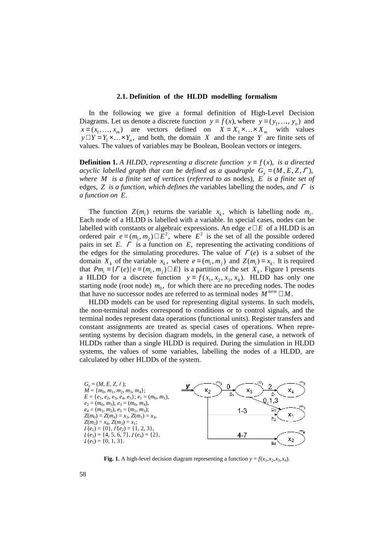
1 2( , ) ,e m m E= ∈ where 2E is the set of all the possible ordered pairs in set .E Γ is a function on ,E representing the activating conditions of the edges for the simulating procedures. The value of ( )eΓ is a subset of the domain kX of the variable ,kx where ( , )i je m m= and ( ) .i kZ m x= It is required that { ( ) | ( , ) }i i jPm e e m m EΓ= = ∈ is a partition of the set .kX Figure 1 presents a HLDD for a discrete function 1 2 3 4( , , , ).y f x x x x= HLDD has only one starting node (root node) 0 ,m for which there are no preceding nodes. The nodes that have no successor nodes are referred to as terminal nodes .termM M∈
HLDD models can be used for representing digital systems. In such models, the non-terminal nodes correspond to conditions or to control signals, and the terminal nodes represent data operations (functional units). Register transfers and constant assignments are treated as special cases of operations. When repre-senting systems by decision diagram models, in the general case, a network of HLDDs rather than a single HLDD is required. During the simulation in HLDD systems, the values of some variables, labelling the nodes of a HLDD, are calculated by other HLDDs of the system.
Fig. 1. A high-level decision diagram representing a function y = f (x1, x2, x3, x4).
Gy = (M, E, Z, Γ); M = {m0, m1, m2, m3, m4}; E = {e1, e2, e3, e4, e5}; e1 = (m0, m1), e2 = (m0, m3), e3 = (m0, m4), e4 = (m1, m2), e5 = (m1, m3); Z(m0) = Z(m4) = x2, Z(m1) = x3, Z(m2) = x4, Z(m3) = x1; Γ(e1) = {0}, Γ(e2) = {1, 2, 3}, Γ(e3) = {4, 5, 6, 7}, Γ(e4) = {2}, Γ(e5) = {0, 1, 3}.
59
(a) (b) (c)
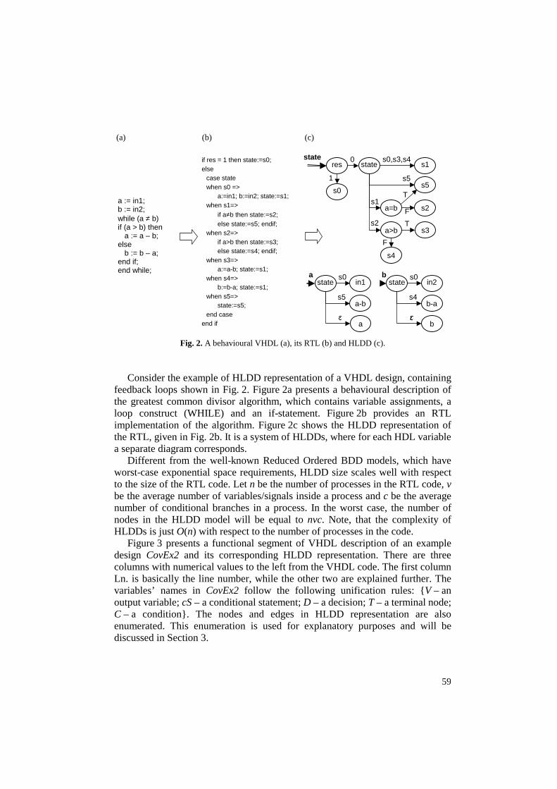
Fig. 2. A behavioural VHDL (a), its RTL (b) and HLDD (c). Consider the example of HLDD representation of a VHDL design, containing
feedback loops shown in Fig. 2. Figure 2a presents a behavioural description of the greatest common divisor algorithm, which contains variable assignments, a loop construct (WHILE) and an if-statement. Figure 2b provides an RTL implementation of the algorithm. Figure 2c shows the HLDD representation of the RTL, given in Fig. 2b. It is a system of HLDDs, where for each HDL variable a separate diagram corresponds.
Different from the well-known Reduced Ordered BDD models, which have worst-case exponential space requirements, HLDD size scales well with respect to the size of the RTL code. Let n be the number of processes in the RTL code, v be the average number of variables/signals inside a process and c be the average number of conditional branches in a process. In the worst case, the number of nodes in the HLDD model will be equal to nvc. Note, that the complexity of HLDDs is just O(n) with respect to the number of processes in the code.
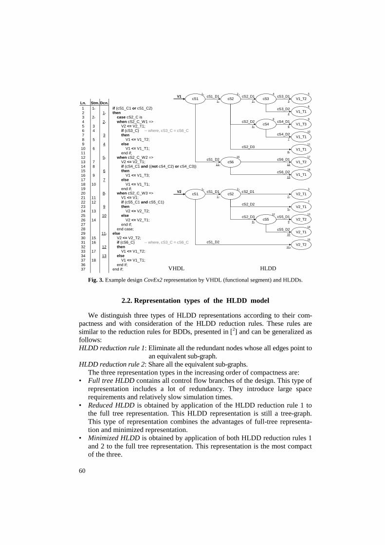
Figure 3 presents a functional segment of VHDL description of an example design CovEx2 and its corresponding HLDD representation. There are three columns with numerical values to the left from the VHDL code. The first column Ln. is basically the line number, while the other two are explained further. The variables’ names in CovEx2 follow the following unification rules: {V – an output variable; cS – a conditional statement; D – a decision; T – a terminal node; C – a condition}. The nodes and edges in HLDD representation are also enumerated. This enumeration is used for explanatory purposes and will be discussed in Section 3.
if res = 1 then state:=s0; else case state when s0 => a:=in1; b:=in2; state:=s1; when s1=>
if a≠b then state:=s2; else state:=s5; endif; when s2=> if a>b then state:=s3; else state:=s4; endif; when s3=> a:=a-b; state:=s1; when s4=> b:=b-a; state:=s1; when s5=> state:=s5; end case end if
state res
0state
s0,s3,s4
s5
s1
a=b
s5
s1
s0
1
s2
T
F
a>b s3 T
F
s4
s2
a state
s0
a-b
in1
s5
a ε
b state
s0
b-a
in2
s4
b ε
a := in1; b := in2; while (a ≠ b) if (a > b) then a := a – b; else b := b – a; end if; end while;
60
Fig. 3. Example design CovEx2 representation by VHDL (functional segment) and HLDDs.
2.2. Representation types of the HLDD model
We distinguish three types of HLDD representations according to their com-pactness and with consideration of the HLDD reduction rules. These rules are similar to the reduction rules for BDDs, presented in [2] and can be generalized as follows: HLDD reduction rule 1: Eliminate all the redundant nodes whose all edges point to
an equivalent sub-graph. HLDD reduction rule 2: Share all the equivalent sub-graphs.
The three representation types in the increasing order of compactness are: • Full tree HLDD contains all control flow branches of the design. This type of
representation includes a lot of redundancy. They introduce large space requirements and relatively slow simulation times.
• Reduced HLDD is obtained by application of the HLDD reduction rule 1 to the full tree representation. This HLDD representation is still a tree-graph. This type of representation combines the advantages of full-tree representa-tion and minimized representation.
• Minimized HLDD is obtained by application of both HLDD reduction rules 1 and 2 to the full tree representation. This representation is the most compact of the three.
Ln. Stm. Dcn. 1
2 3 4 5 6 7 8 9
10 11 12 13 14 15 16 17 18 19 20 21 22 23 24 25 26 27 28 29 30 31 32 33 34 37 36 37
1*
2*
3 4
5
6
7 8
9
10
11 12
13
14
15 16
17
18
1*
2*
3
4
5*
6
7
8*
9
10
11*
12
13
if (cS1_C1 or cS1_C2) then case cS2_C is when cS2_C_W1 => V2 <= V2_T1; if (cS3_C) -- where, cS3_C = cS6_C then V1 <= V1_T2; else V1 <= V1_T1; end if; when cS2_C_W2 => V2 <= V2_T1; if (cS4_C1 and ((not cS4_C2) or cS4_C3)) then V1 <= V1_T3; else V1 <= V1_T1; end if; when cS2_C_W3 => V1 <= V1; if (cS5_C1 and cS5_C1) then V2 <= V2_T2; else V2 <= V2_T1; end if; end case; else V2 <= V2_T2; if (cS6_C) -- where, cS3_C = cS6_C then V1 <= V1_T2; else V1 <= V1_T1; end if; end if; VHDL HLDD
cS1_D1 cS2_D1
cS2_D2
cS3_D1
cS3_D2
cS1_D2
cS4_D1
cS4_D2
cS1 cS2 cS3 V1_T2
V1_T1
cS4 V1_T3
V1_T1
V1
cS6_D1
cS6_D2
cS6 V1_T2
V1_T1
11 3
7
21
4
651
12111
13
11 21 5
6
9
10
17
18
8
16
4
cS2_D3V1_T1
81
11
cS1_D1 cS2_D1
cS2_D3 cS5_D1
cS5_D2
cS1_D2
cS1 cS2 V2_T1
cS5 V2_T2
V2_T1
V2_T2
V2
82
10
112
9
2212
3
13
14
15
12
2212
cS2_D2V2_T1
52
7
61
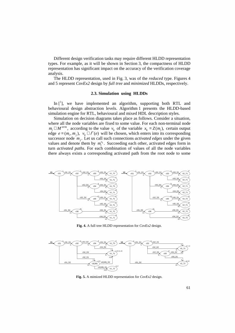
Different design verification tasks may require different HLDD representation types. For example, as it will be shown in Section 3, the compactness of HLDD representation has significant impact on the accuracy of the verification coverage analysis.
The HLDD representation, used in Fig. 3, was of the reduced type. Figures 4 and 5 represent CovEx2 design by full tree and minimized HLDDs, respectively.
2.3. Simulation using HLDDs
In [1], we have implemented an algorithm, supporting both RTL and
behavioural design abstraction levels. Algorithm 1 presents the HLDD-based simulation engine for RTL, behavioural and mixed HDL description styles.
Simulation on decision diagrams takes place as follows. Consider a situation, where all the node variables are fixed to some value. For each non-terminal node
,termim M∉ according to the value kv of the variable ( ),k ix Z m= certain output
edge ( , ),i je m m= ( )kv eΓ∈ will be chosen, which enters into its corresponding successor node .jm Let us call such connections activated edges under the given values and denote them by .kv
im Succeeding each other, activated edges form in turn activated paths. For each combination of values of all the node variables there always exists a corresponding activated path from the root node to some
Fig. 4. A full tree HLDD representation for CovEx2 design.
Fig. 5. A mimized HLDD representation for CovEx2 design.
cS1_D1
cS2_D1
cS2_D2
cS(3/6)_D1
cS(3/6)_D2cS1_D2
cS4_D1
cS4_D2
cS1 cS2
cS(3/6)
V1_T2
cS4 V1_T3V1
11
3,12
7
111
4,13
651
21
11 21
5,17
98
4,16
cS2_D3V1_T1
81
6,10,11,18
cS1_D1 cS2_D1
cS2_D3
cS1_D2
cS1 cS2
cS5
V2_T2
V2
82
10
9
2212
13,15
2212
cS2_D2V2_T1
52
3,7,14
cS5_D212
cS5_D1
112
11d
11d
cS1_D1 cS2_D1
cS2_D2
cS3_D1
cS3_D2
cS1_D2
cS4_D1
cS4_D2
cS1 cS2 cS3 V1_T2
V1_T1
cS4 V1_T3
V1_T1
V1
cS6_D1
cS6_D2
cS6 V1_T2
V1_T1
11 31
71
21
41
6151
121111
131
11 21 5
6
9
10
17
18
81
161
41
cS2_D3 cS5_D1
cS5_D2
cS5 V1_T1
V1_T1
81
101
91
121
7d
7d
15d
15d
3d
3d
cS1_D1 cS2_D1
cS2_D2
cS3_D1
cS3_D2
cS1_D2
cS4_D1
cS4_D2
cS1 cS2 cS3 V2_T1
V2_T1
cS4 V2_T1
V2_T1
V2
cS6_D1
cS6_D2
cS6 V2_T2
V2_T2
12 32
72
22
42
6252
122112
132
12 22
82
162
42
cS2_D3 cS5_D1
cS5_D2
cS5 V2_T2
V2_T1
82
102
92
13
14
122
62
terminal node. We refer to this path as the main activated path. The simulated value of variable, represented by the HLDD, will be the value of the variable labelling the terminal node of the main activated path. Algorithm 1. SimulateHLDD() For each diagram G in the model mCurrent = m0 Let xCurrent be the variable labeling mCurrent While mCurrent is not a terminal node If xCurrent is clocked or its DD is ranked after G then Value = previous time-step value of xCurrent Else Value = present time-step value of xCurrent End if mCurrent = mCurrent
Value
End while Assign xG = xCurrent End for End SimulateHLDD
In the RTL style, the algorithm takes the previous time step value of variable ,jx labelling a node ,im if jx represents a clocked variable in the corresponding
HDL. Otherwise, the present value of jx will be used. In the case of behavioural HDL coding style, HLDDs are generated and ranked in a specific order to ensure causality. For variables ,jx labelling HLDD nodes the previous time step value is used if the HLDD calculating jx is ranked after the current decision diagram. Otherwise, the present time step value will be used.
Let us explain the HLDD simulation process on the decision diagram example, presented in Fig. 1. Assuming that variable 2x is equal to 2, a path is activated from node 0m (the root node) to a terminal node 3,m labelled with 1.x Let the value of variable 1x be 4, thus, 1 4.y x= = Note, that this type of simulation is event-driven since we have to simulate only those nodes that are traversed by the main activated path.
3. HLDD-BASED COVERAGE ANALYSIS Hardware verification coverage analysis is aimed to estimate quality and
completeness of the performed verification. It plays a key role in simulation-based verification and helps to find an answer to the important yet sophisticated question of when the design is verified enough. The main focus in this paper is on the structural coverage (code coverage) for simulation-based verification as the most widely used in practice. This section describes how a number of traditional code coverage metrics [6,7] can be analysed, based on the HLDD model.
63
3.1. Statement coverage analysis The statement coverage is the ratio of statements, executed during simulation,
to the total number of statements under the given set of stimuli. The idea of statement coverage representation on HLDDs was proposed in [8]
and developed further in [9]. The statement coverage metric has a straightforward mapping to HLDD-based coverage. It maps directly to the ratio of nodes mCurrent, traversed during the HLDD simulation presented in Algorithm 1 (Sub-section 2.3), to the total number of the HLDD nodes in the DUV’s (Design Under Verification) representation. The appropriate type of HLDD representation for the analysis of both, statement and branch coverage metrics, is the reduced one. The variations in the analysis, caused by different HLDD representation types, are discussed further.
Let us consider the VHDL description of the CovEx2 design, provided in Fig. 3. The numbers in the second column (Stm.) correspond to the lines with statements (both conditional and assignment). The 20 HLDD nodes of the two graphs in the same figure correspond to the 18 statements of the VHDL segment. Covering all nodes in the HLDD model (i.e. full HLDD node coverage) corresponds to covering all statements in the respective HDL (100% statement coverage). However, the opposite is not true. HLDD node coverage is slightly more stringent than HDL statement coverage. Please note that some of the HDL statements have duplicated representation by the HLDD nodes. This is due to the fact that HLDD diagrams are normally generated for each data variable separately. Please consider statements 1 and 2 with asterisk ‘*’ in VHDL representation and additional indexes in HLDD (Fig. 3). They are represented twice by the nodes of both variables V1 and V2 graphs, and therefore there are 20 HLDD nodes in total.
The fact that HLDD node coverage is slightly more stringent than HDL statement coverage is caused by their property to better represent the actual structure of the design. For example, if one statement in a design description by VHDL can be accessed by several execution paths, it will be represented by a number of nodes (or sub-graphs) in the corresponding graph when reduced, or full-tree HLDD representations are used.
3.2. Branch coverage analysis
The branch coverage metric shows the ratio of branches in the control flow
graph of the code that are traversed under the given set of stimuli. This metric is also known as decision coverage, especially in software testing [7], and arc coverage. In a typical application of branch coverage measurement, the number of every decision’s hits is counted. Note, that the full branch coverage comprises full statement coverage.
Similar to the statement coverage, branch coverage also has very clear representation in the HLDD model (also initially proposed in [8] and developed
64
further in [9]). It is the ratio of every edge eactive, activated in the simulation process, presented by Algorithm 1 (Subsection 2.3) to the total number of edges in the corresponding HLDD representation of the DUV.
Let us consider the VHDL segment in Fig. 3. Here, the third column (Dcn.) numbers all 13 branches (aka decisions) of the code. The edges in the HLDD graphs, provided in Fig. 3, represent these branches and are marked by the corresponding numbers (underlined). Covering all the edges in a HLDD model (i.e. full HLDD edge coverage) corresponds to covering all branches in the respective HDL. However, similarly to the previously discussed statement on coverage mapping, here the opposite is also not true and HLDD edge coverage is slightly more stringent than HDL branch coverage.
Please note that some of the HDL branches also have duplicated repre-sentation by the HLDD edges. This is due to the same reason as with HLDD nodes. In Fig. 3 they are marked by ‘*’ and by additional subscript indexes.
The HLDD-based approaches for statement and branch coverage metrics can further be extended for other metrics of structural verification coverage such as state coverage (aka FSM coverage), data flow coverage and others. In the first case the graph or graphs for the state variable should be analysed. The second one would require strict HLDD model partitioning by the variables sub-graphs and would map to the coverage of all single paths from terminal nodes to the root nodes separately in all variables’ HLDD sub-graphs.
3.3. Condition coverage analysis
Condition coverage metric reports all cases of each Boolean sub-expression,
separated by logical operators or and and; in a conditional statement it causes the complete conditional statement to evaluate the decisions (e.g. ‘true’ or ‘false’ values) under the given set of stimuli. It differs from the branch coverage by the fact that in the branch coverage only the final decision, determining the branch, is taken into account. If we have n conditions, joined by logical and operators in a logical expression of a conditional statement, it means that the probability of evaluating the statement to the decision ‘true’ is 1/2n (considering pure random stimuli for the condition values). Calculation of the condition coverage, based on HDL representation, is a sophisticated multi-step process. However, the condi-tion coverage metric allows discovering information about many corner cases of the DUV.
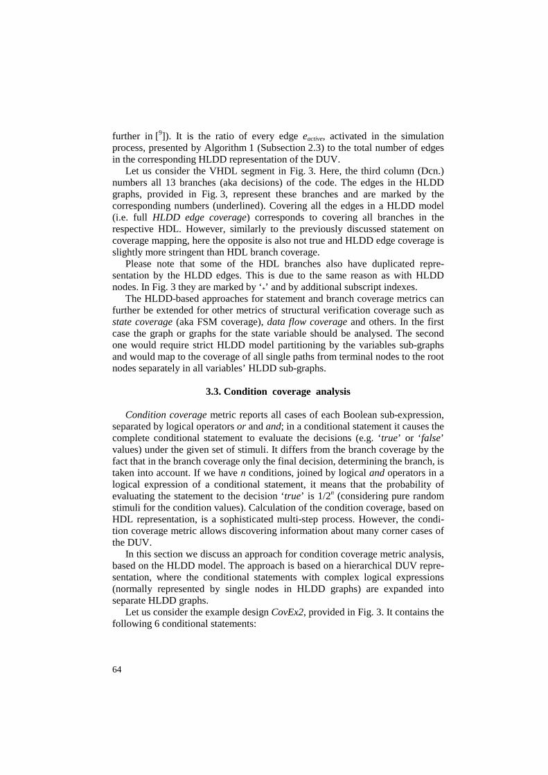
In this section we discuss an approach for condition coverage metric analysis, based on the HLDD model. The approach is based on a hierarchical DUV repre-sentation, where the conditional statements with complex logical expressions (normally represented by single nodes in HLDD graphs) are expanded into separate HLDD graphs.
Let us consider the example design CovEx2, provided in Fig. 3. It contains the following 6 conditional statements:
65
cS1: if (cS1_C1 or cS1_C2) then cS1_D1 else cS1_D2;
cS2: case (cS2_C) when cS2_C_W1: cS2_D1;
when cS2_C_W2: cS2_D2;
when cS2_C_W3: cS2_D3;
cS3: if (cS3_C) then cS3_D1 else cS3_D2; -- where, cS3_C = cS6_C
cS4: if (cS4_C1 and ((not cS5_C2) or cS5_C3))then cS4_D1 else cS4_D2;
cS5: if (cS5_C1 and cS5_C2) then cS5_D1 else cS5_D2;
cS6: if (cS6_C) then cS6_D1 else cS6_D2; -- where, cS3_C = cS6_C
The HLDD expansion graphs for these conditional statements are provided in
Fig. 6. Here the terminal nodes are marked by background colors according to different decisions for better readability.
These 6 expansion graphs can be considered as sub-graphs, representing “virtual” variables (because they are not real variables of the CovEx2 VHDL representation) cS1–cS6. Thus together with the two HLDD graphs for variables V1 and V2 (Fig. 3) these sub-graphs compose hierarchical HLDD representation of the design (altogether 8 graphs). Here we choose graphs from Fig. 3, because accurate condition coverage analysis requires reduced type of HLDDs.
The full condition coverage metric maps to the full coverage of terminal nodes of the conditional statements expansion graphs during the complete
Fig. 6. Expansion graphs for conditional statements of CovEx2.
T
F
cS1_C1
cS1_D2
cS1cS1_C2
cS1_C2T
cS1_D1F
cS1_D1
cS1_D1F
T
TcS4_C1
cS4cS4_C2
F
cS4_D1T
T
F
cS5_C1
cS5_D2
cS5cS5_C2
cS5_C2T
cS5_D2F
cS5_D1
cS5_D2F
T
TcS4_C3
cS4_D2F
cS4_D1TF
cS4_C3
cS4_D1F
cS4_C2 cS4_D2TT
cS4_C3
cS4_D2F
cS4_D2TF
cS4_C3
cS4_D2F
cS2_C_W1
cS2_C_W2
cS2_C
cS2_D2
cS2cS2_D1
cS2_C_W3cS2_D3
T
F
cS6_C
cS6_D2
cS6cS6_D1
T
F
cS3_C
cS3_D2
cS3cS3_D1
66
hierarchical DD system simulation with the given stimuli. The size of the items’ list CI for this coverage metric is:
1 1
2 .cScS CASEIF
ci
k
nnn
C ci k
I n= =
= +∑ ∑
Here
IFcSn is the number of if-type conditional statements, icn is the number
of conditions in the ith conditional statement, CASEcSn is the number of case-type
conditional statements and kcn is the number of conditions in the kth conditional
statement. E.g., list of the condition coverage items for СovEx2 is 1 2 3(2* 2 2* 2 2 ) (3) 23.CI = + + + =
The main advantage of the proposed approach is low computational overhead. Once the hierarchical HLDD is constructed, the analysis for every given stimuli set is evaluated in a straightforward manner during HLDD simulation (Algorithm 1, Subsection 2.3).
The size of the hierarchical HLDDs with the expanded conditional statements grows with respect to CI and therefore there is a significant increase of the memory consumption. However, the length of the average sub-path from the root to terminal nodes grows linearly with the number of conditions. Therefore, since the simulation time of a HLDD has a linear dependence on the average sub-path from the root to terminal nodes, it will grow only linearly with respect to the number of conditions.
A less compact HLDD representation contains more items, i.e. nodes and edges. It means it requires more memory for the data structure storage and possibly longer simulation time, if the average sub-path from the root to terminal nodes becomes longer. However, it is potentially capable to represent the design’s structure more accurately and therefore the coverage measurement may be more accurate as well.
It has been shown in [10] that the results of the analysis of the discussed coverage metrics, performed on reduced HLDDs, are more stringent that the ones with the minimized HLDDs. Moreover, compared to HDL-based analysis, the reduced HLDD-based results are always more stringent, while minimized HLDD-based ones are often less.
At the same time, the performance of the base coverage metrics analyses, based on the reduced and minimized HLDD model, is equivalent due to the fact that both models have the same average length of sub-paths from the root to terminal nodes. Compared to the full tree HLDD representation, the reduced HLDD model usually has significant performance improvement while the accuracy of the design’s structure representation remains the same for the discussed coverage metrics.
67
4. HLDD-BASED ASSERTION CHECKING Application of assertions checking has been recognized to be an efficient
technique in many steps of the state-of-the-art digital systems design [11]. In simulation-based verification, which is the main focus of this paper, assertions play the role of monitors for a particular system behaviour during simulation and signal about satisfaction or violation of the property of interest [12].
The popularity of assertion-based verification has encouraged cooperative development of a language, specially dedicated for assertions expression. As a result, a Property Specification Language (PSL), which is based on IBM’s language Sugar, has been introduced [13]. Later it has become an IEEE 1850 Standard [14]. PSL has been specifically designed to fulfill several general functional specification requirements for hardware, such as ease of use, concise syntax, well-defined formal semantics, expressive power and known efficient underlying algorithms in simulation-based verification. Research on the topic of converting PSL assertions to various design representations, such as finite state machines and hardware description languages, is gaining popularity [15–18]. Probably the most well-known commercial tool for this task is FoCs [19] by IBM. The above-mentioned solutions and the approach proposed in [20] mainly address synthesis of checkers from PSL properties that are to be used in hardware emulation. The application of the same checker constructs for simulation in software may lack efficiency due to target language concurrency and poor means for temporal expressions. Current approach allows avoiding the above limitations. The structure of an HLDD design representation with the temporal extension, proposed in this paper, allows straightforward and lossless translation of PSL properties. Traditionally the process of checking complex temporal assertions in HDL environment causes significant time and resources overhead. In this section, we discuss an approach to checking PSL assertions using HLDDs that is aimed to overcome these drawbacks.
4.1. PSL for assertion expression
The PSL [13,21] is a multi-flavored language. In this paper we consider only its
VHDL flavour. PSL is also a multi-layered language. The layers include: • Boolean layer – the lowest one, consists of Boolean expressions in HDL (e.g.
a &&(b || c)) • Temporal layer – sequences of Boolean expressions over multiple clock
cycles, also supports Sequential Extended Regular Expressions (SERE) (e.g. {A[*3];B} |-> {C})
• Verification layer – it provides directives that tell a verification tool what to do with the specified sequences and properties.
• Modelling layer – additional helper code to model auxiliary combinational signals, state machines etc that are not part of the actual design but are required to express the property.
68
The temporal layer of the PSL language has two constituents: • Foundation Language (FL) that is Linear time Temporal Logic (LTL) with
embedded SERE • Optional Branching Extension (OBE) that is Computational Tree Logic
(CTL) The latter considers multiple execution paths and models design behaviour as
execution trees. The OBE part of PSL is normally applied for formal verification. Therefore, in this paper we shall consider only the FL part of PSL. In fact, only FL, or more precisely, its subset known as PSL Simple Subset, is suitable for dynamic assertion checking. This subset is explicitly defined in [139] and loosely speaking it has two requirements for time: to advance monotonically and to be finite, which leads to restrictions on types of operands for several operators. Currently in the discussed HLDD-based approach only several LTL operators without SERE support are implemented. However, as it will be shown later, the support for SERE as well as for any other language constructs can be easily added by an appropriate library extension.
Let us consider a simple example assertion, expressed in PSL: reqack: assert always (req -> next ack).
Here reqack followed by semicolon is a label that provides a name for the assertion. assert is a verification directive from the Verification layer, always and next are temporal operators, ->is an operator from Boolean layer, while req and ack are Boolean operands that are also 2 signals in the DUV.
In the following the reqack assertion checking results are shown for 3 example stimuli sequences for signals {req, ack}: • stimuli 1: ({0,0};{1,0};{0,1} {0,0}) - PASS (satisfied) • stimuli 2: ({0,0};{1,0};{0,0} {0,0}) - FAIL (violated) • stimuli 3: ({0,0};{0,0};{0,1} {0,0}) - not activated (vacuous pass)
Vacuous pass occurs if a passing property contains Boolean expression that, in frames of the given simulation trace, has no effect on the property evaluation. The property has passed not because of meeting all the specified behaviour but only because of non-fulfillment of logical implication activation conditions. The decision whether to treat vacuous passes as actual satisfactions of properties or not depends on particular verification tool. The approaches presented in this paper separate vacuous passes from normal passes of a property.
4.2. Temporally extended HLDDs
In order to support complex temporal constructs of PSL assertion, an
extension for the HLDD modelling formalism has been proposed [22]. The extension is referred to as temporally extended high-level decision diagrams (THLDDs).
Unlike the traditional HLDD, the temporally extended high-level decision diagrams are aimed at representing temporal logic properties. A temporal logic property P at the time-step ,ht T∈ denoted by ( , ),
htP f x T= where
1( , , ),mx x x= K is a Boolean vector and 1{ , , )sT t t= K is a finite set of time-
69
steps. In order to represent the temporal logic assertion ( , ),ht
P f x T= a temporally extended high-level decision diagram PG can be used. Definition 2. A temporally extended high-level decision diagram (THLDD) is a non-cyclic directed labelled graph that can be defined as a sixtuple
( , , , , , ),PG M E T Z Γ Φ= where M is a finite set of nodes, E is a finite set of edges, T is a finite set of time-steps, Z is a function, which defines the variables, labelling the nodes and their domains, Γ is a function on ,E repre-senting the activating conditions for the edges, and Φ is a function on M and
,T defining temporal relationships for the labelling variables.
The graph PG has exactly three terminal nodes ,termM M∈ labelled with constants, whose semantics is explained below: • FAIL – the assertion P has been simulated and does not hold; • PASS – the assertion P has been simulated and holds; • CHK. (from CHECKING) – the assertion P has been simulated and it does
not fail, nor does it pass non-vacuously. The function ( , )im tΦ represents the relationship, indicating at which time-
steps t T∈ the node labelling variable ( )l ix Z m= should be evaluated. More exactly, the function returns the range of time-steps relative to current time ,currt where the value of variable kx must be read. We denote the relative time range by t∆ and calculation of variable lx using the time-range ( , )im t tΦ = ∆ by .t
lx∆ We distinguish three cases: • { , , },t j k∆ = ∀ K meaning that tj tk
l lx x∆ ∆∧ ∧K is true, i.e. variable lx is true at every time-step between curr jt + and .curr kt +
• { , , },t j k∆ = ∃ K meaning that tj tkl lx x∆ ∆∨ ∨K is true, i.e. variable lx is true
at least at one of the time-steps between curr jt + and .curr kt + • ,t k∆ = where k is a constant. In other words, the variable lx has to be true
k time-steps from current time-step .currt In fact, t k∆ = is equivalent to and may be represented by { , , },t k k∆ = ∀ K or alternatively by { , , }.t k k∆ = ∃ K Notation ( )cevent x is a special case of the upper bound of the time range,
denoted above by k and means the first time-step when cx becomes true. This notation can be used in the three listed above THLDD temporal relationship functions ( , ),im tΦ which creates the listed below variations of them. For ,t
lx∆ where lx and cx are node labelling variables: • {0, , ( )},ct event x∆ = ∀ K which means that variable lx is true at every time-
step between currt and the first time-step from currt when variable cx becomes true, inclusively. This is equivalent to the PSL expression lx until_ .cx The PSL expression lx until_ cx can be represented by t∆ =
{0, , ( ) 1}.cevent x∀ −K • {0, , ( )},ct event x∆ = ∃ K which means that variable lx is true at least at one of
the time-steps between currt and the first time-step from currt when variable
cx becomes true, inclusive. This is equivalent to the PSL expression lx before_ .cx The PSL expression lx before_ cx can be represented by
{0, , ( ) 1}.ct event x∆ = ∃ −K
70
• ( ),ct event x∆ = which means that variable lx has to be true at the first time-step when cx becomes true. This is equivalent to the PSL expression
_ ( ) .c lnext event x x For Boolean, i.e. non-temporal, variables 0.t∆ = Table 1 shows examples on how temporal relationships in THLDDs map to
PSL expressions. In addition, we use the notion of endt as a special value for the upper bound of
the time range, denoted above by ;k endt is the final time-step that occurs at the end of simulation and is determined by one of the following cases: • number of test vectors • the amount of time provided for simulation • simulation interruption
The special values for the time range bounds (i.e. ( )cevent x and )endt are supported by the HLDD-based assertion checking process. In the proposed approach the design simulation, which calculates simulation trace, precedes assertion checking process. In practice, endt is the final time-step of the pre-stored simulation trace.
Note, that THLDD is an extension of HLDD, defined in Section 2, as it includes temporal relationships functions. The main purpose of the proposed temporal extension is transferring additional information and giving directives to the HLDD simulator that will be used for assertions checking.
4.3. PSL assertions conversion to THLDDs
The first step in the conversion process is parsing a PSL assertion of interest
into elementary entities, containing one operator only. The hierarchy of operators is determined by the PSL operators precedence specified by the IEEE1850 Standard. The second step is generation of a THLDD representation for the assertion. This process in turn consists of two stages. The first stage is preparatory and consists of a PPG (Primitive Property Graphs) library creation for elementary operators. The second stage is recursive hierarchical construction of a THLDD graph for a complex property using the PPG library elements.
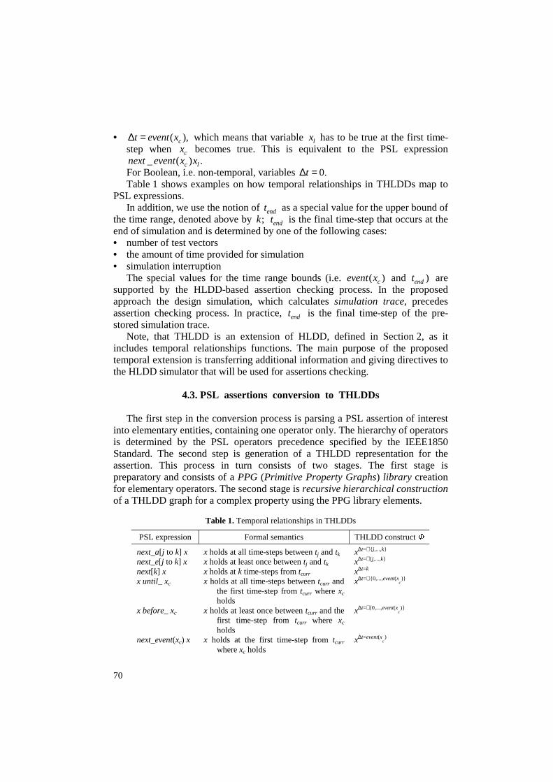
Table 1. Temporal relationships in THLDDs
PSL expression Formal semantics THLDD construct Φ
next_a[j to k] x x holds at all time-steps between tj and tk x∆t=∀ {j,...,k} next_e[j to k] x x holds at least once between tj and tk x∆t=∃ {j,...,k} next[k] x x holds at k time-steps from tcurr x∆t=k x until_ xc x holds at all time-steps between tcurr and
the first time-step from tcurr where xc holds
x∆t=∀ {0,...,event(xc )}
x before_ xc x holds at least once between tcurr and the first time-step from tcurr where xc holds
x∆t=∃ {0,...,event(xc )}
next_event(xc) x x holds at the first time-step from tcurr where xc holds
x∆t=event(xc )
71
A PPG should be created for every PSL operator supported by the proposed approach. All the created PPGs are combined into one PPG Library. The library is extensible and should be created only once. It implicitly determines the supported PSL subset. The method currently supports only weak versions of PSL FL LTL-style operators. However, by means of the supported operators a large set of properties, expressed in PSL, can be derived. Primitive property graph is always a THLDD graph. That means it uses HLDD model with the proposed above temporal extension and has a standard interface.
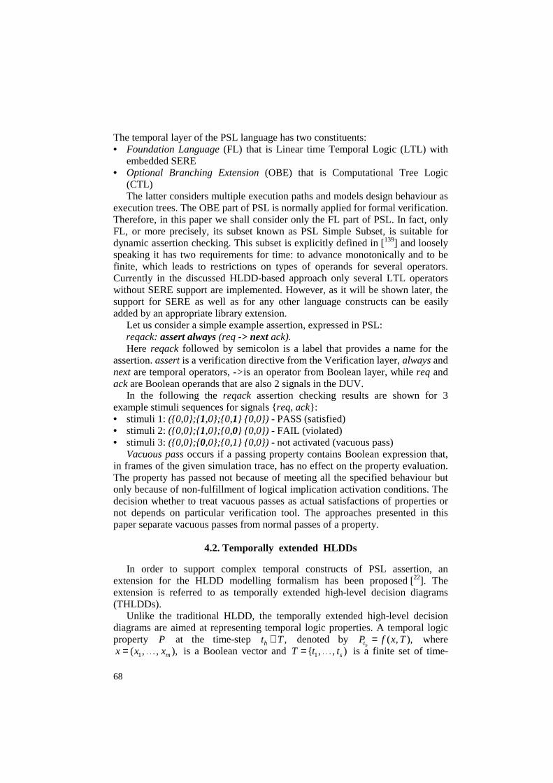
Figure 7 shows examples of primitive property graphs for two PSL operators next_e and logical implication ->.
The construction of complex THLDD properties is performed in the top-down manner. The process starts from the operators with the lowest precedence, forming the top level. Then their operands that are sub-operators with higher precedence recursively form lower levels of the complex property. For example, always and never operators have the lowest level of precedence and consequently their corresponding PPGs are put to the highest level in the hierarchy. The sub-properties (operands) are step-by-step substituted by lower level PPGs until the lowest level, where sub-properties are pure signals or HDL operations.
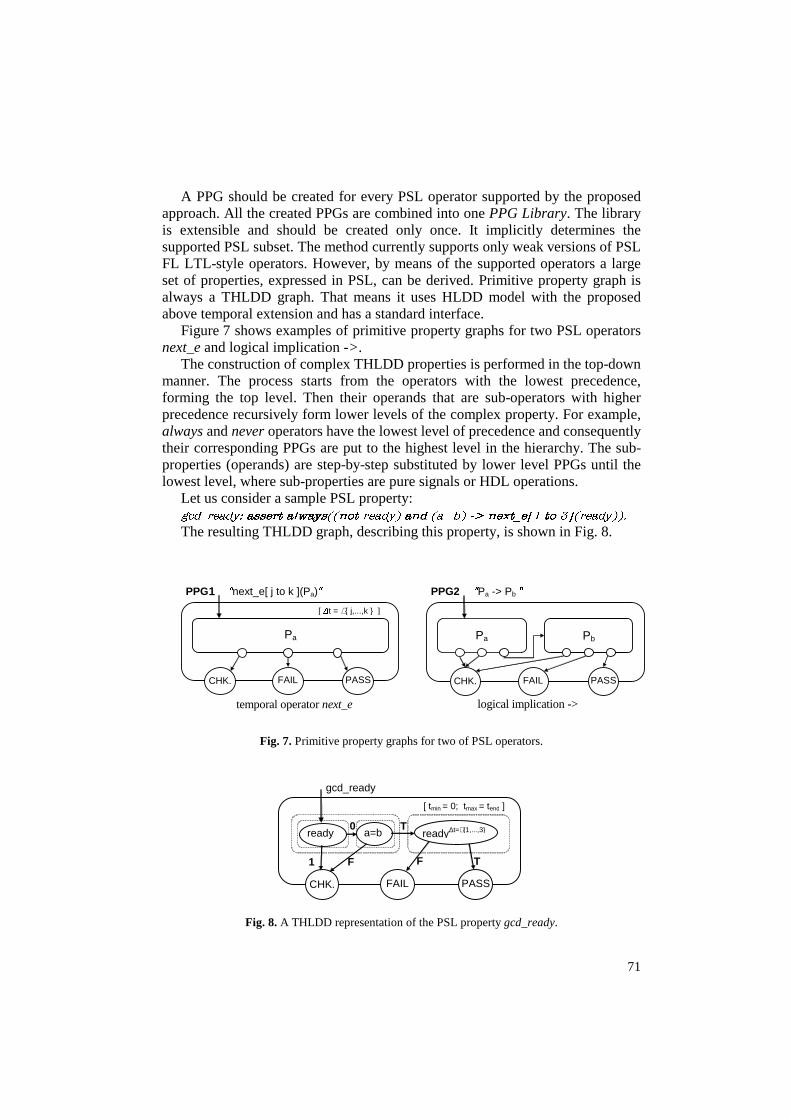
Let us consider a sample PSL property: gcd_ready: assert always((not ready) and (a=b) -> next_e[1 to 3](ready)).
The resulting THLDD graph, describing this property, is shown in Fig. 8.
Fig. 7. Primitive property graphs for two of PSL operators.
Fig. 8. A THLDD representation of the PSL property gcd_ready.
PPG2 ″Pa -> Pb ″
FAIL PASS CHK.
Pa Pb
logical implication -> temporal operator next_e
PPG3 ″next_e[ j to k ](Pa)″
[ ∆t = ∃ { j,...,k } ]
FAIL PASS CHK.
Pa
1
1 T
ready a=b ready∆t=∃ {1,...,3}
gcd_ready
[ tmin = 0; tmax = tend ]
FAIL PASS CHK.
0
F F
T
72
The construction of the property gcd_ready implies usage of the four PPGs. The nodes in the final THLDD contain signal variables and an HDL expression (a = b).
4.4. HLDD-based assertion checking
The process of HLDD-based assertion checking implies the existing HLDD
simulator functionality (Algorithm 1) and its extension for assertion checking presented by Algorithm 2.
In the current implementation, HLDD-based assertion checking is a two-step process. First the DUV has to be simulated (Algorithm 1, Section 2.3), which calculates the simulation trace. This trace is a starting point for assertion checking that is performed in accordance with Algorithm 2 shown bellow. The process of checking takes into account temporal relationships information at the THLD nodes that represent an assertion.
Algorithm 2. AssertionCheck() For each diagram G in the model For t=tmin...tmax mCurrent = m0 ; tnow = t xCurrent = Z(mCurrent) Repeat If tnow > tmax then Exit End if Value = xCurrent at Φ(mCurrent,tnow) mCurrent = mCurrent
Value
tnow = tnow+∆t
Until mCurrent ∉ Mterm Assign xG = xCurrent at time-step tnow End for /* t= tmin...tmax */ End for End AssertionCheck
A general flow of the HLDD-based assertion checking process can be described as follows. The input data for the first step (simulation) are HLDD model representation of the design under verification and stimuli. This step results in a simulation trace, stored in a text file. The second step (checking) uses this data as well as the set of THLDD assertions as input. The output of the second step is the assertions checking results that include information about both the assertions coverage and their validity.
The stored assertion validity data allows further analysis and reasoning of which combinations of stimuli and design states have caused fails and passes of the assertions. This data also implicitly contains information about the monitored asser-tions coverage (i.e. assertion activity: “active” or “inactive”) by the given stimuli.
73
5. EXPERIMENTAL RESULTS This section demonstrates experimental results for the discussed HLDD
model applications for verification coverage analysis and assertion checking. The experiment benchmarks several designs from ITC’99 benchmarks family [23] and a design gcd which is an implementation of the greatest common devisor.
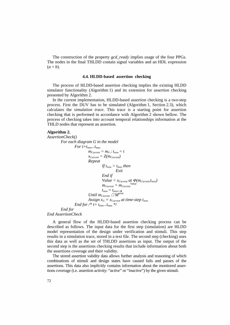
Figure 9 shows comparison results obtained in [10] with the proposed methodology, based on different HLDD representations and coverage analysis, achieved by a commercial state-of-the-art HDL simulation tool from a major CAD vendor using the same sets of stimuli.
As it can be seen, the reduced HLDDs with expanded conditional nodes allow equal or more stringent coverage evaluation in comparison to the commercial coverage analysis software. For three designs (b01, b06 and b09) more stringent analysis is achieved using HLDDs. The HLDD model allows increasing the coverage accuracy up to 13% more exact statement measurement and 14% branch measurement (b09 design). While minimized HLDD require less memory compared to the reduced type, they do not suit accurate coverage analysis. Please note, that a higher coverage percentage, reported by a coverage metric for the given stimuli, means the metric is less stringent compared to another showing more potential for stimuli improvement and thus being more accurate.
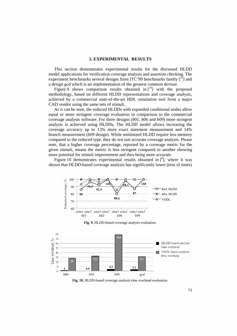
Figure 10 demonstrates experimental results obtained in [8], where it was shown that HLDD-based coverage analysis has significantly lower (tens of times)
Fig. 9. HLDD-based coverage analysis evaluation.
Fig. 10. HLDD-based coverage analysis time overhead evaluation.
74
computation (i.e. measurement) time overhead compared to the same commercial simulator.
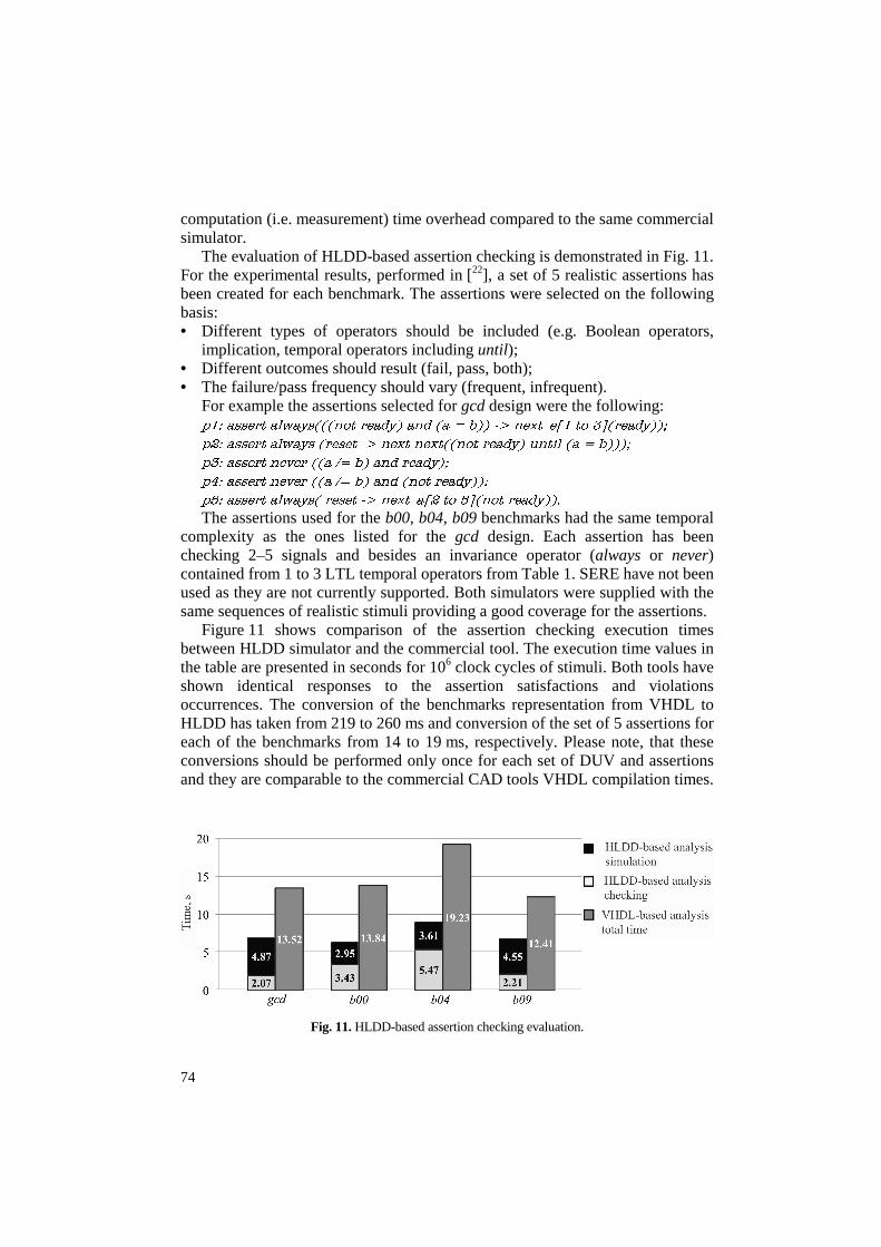
The evaluation of HLDD-based assertion checking is demonstrated in Fig. 11. For the experimental results, performed in [22], a set of 5 realistic assertions has been created for each benchmark. The assertions were selected on the following basis: • Different types of operators should be included (e.g. Boolean operators,
implication, temporal operators including until); • Different outcomes should result (fail, pass, both); • The failure/pass frequency should vary (frequent, infrequent).
For example the assertions selected for gcd design were the following: p1: assert always(((not ready) and (a = b)) -> next_e[1 to 3](ready));
p2: assert always (reset -> next next((not ready) until (a = b)));
p3: assert never ((a /= b) and ready);
p4: assert never ((a /= b) and (not ready));
p5: assert always( reset -> next_a[2 to 5](not ready)).
The assertions used for the b00, b04, b09 benchmarks had the same temporal complexity as the ones listed for the gcd design. Each assertion has been checking 2–5 signals and besides an invariance operator (always or never) contained from 1 to 3 LTL temporal operators from Table 1. SERE have not been used as they are not currently supported. Both simulators were supplied with the same sequences of realistic stimuli providing a good coverage for the assertions.
Figure 11 shows comparison of the assertion checking execution times between HLDD simulator and the commercial tool. The execution time values in the table are presented in seconds for 106 clock cycles of stimuli. Both tools have shown identical responses to the assertion satisfactions and violations occurrences. The conversion of the benchmarks representation from VHDL to HLDD has taken from 219 to 260 ms and conversion of the set of 5 assertions for each of the benchmarks from 14 to 19 ms, respectively. Please note, that these conversions should be performed only once for each set of DUV and assertions and they are comparable to the commercial CAD tools VHDL compilation times.
Fig. 11. HLDD-based assertion checking evaluation.
75
During the experiments we have tried to use different number of time intervals with various sizes and have not observed any issues with scalability, however, proper experiments to evaluate the scalability issue are scheduled for the future.
The presented experimental results show the feasibility of the proposed approach and a significant speed-up (2 times) in the execution time, required for design simulation with assertion checking by the proposed approach compared to the state-of-the-art commercial tool.
6. CONCLUSIONS This paper has demonstrated several advantages of the application of high-
level decision diagrams for simulation-based verification. The paper has discussed an approach to the structural coverage analysis using
HLDDs. In particular, statement, branch and condition coverage metrics have been considered in details. It is important to emphasize that all coverage metrics (i.e. statement, branch, condition or a combination of them) in the proposed methodology are analysed by a single HLDD simulation tool which relies on HLDD design representation model. Different levels of coverages are distinguished by simply generating a different level of HLDD (i.e. minimized, reduced, or hierarchical with expanded conditional nodes).
An HLDD-based approach for assertion checking has also been demonstrated. The approach implies a temporal extension of HLDD model (THLDD) to support temporal operations inherent in IEEE standard PSL properties and also to directly support assertion checking. A hierarchical approach to generate THLDDs and basic algorithms for THLDD-based assertion checking were discussed.
As a future work we see integration of these HLDD-based assertion checking and coverage measurement methods for the design error diagnosis and debug solutions.
ACKNOWLEDGEMENTS This work has been supported by European Commission Framework Program
7 projects DIAMOND and CREDES, by European Union through the European Regional Development Fund, by Estonian Science Foundation (grants Nos. 8478, 7068 and 7483), Enterprise Estonia funded ELIKO Development Centre and Estonian Information Technology Foundation (EITSA).
REFERENCES
1. Ubar, R., Raik, J. and Morawiec, A. Back-tracing and event-driven techniques in high-level simulation with decision diagrams. In Proc. IEEE International Symposium on Circuits and Systems. Geneva, 2000, 208–211.
76
2. Bryant, R. E. Graph-based algorithms for boolean function manipulation. IEEE Trans. Computers, 1986, C-35, 677–691.
3. Clarke, E., Fujita, M., McGeer, P., McMillan, K. L., Yang, J. and Zhao, X. Multi terminal BDDs: an efficient data structure for matrix representation. In Proc. International Work-shop on Logic Synthesis, Louvain, Belgium, 1993, 1–15.
4. Drechsler, R., Becker, B. and Ruppertz, S. K *BMDs: a new data structure for verification. In Proc. European Design & Test Conference, Paris, 1996, 2–8.
5. Chayakul, V., Gajski, D. D. and Ramachandran, L. High-level transformations for minimizing syntactic variances. In Proc. ACM IEEE Design Automation Conference. Texas, TX, 1993, 413–441.
6. Piziali, A. Functional Verification Coverage Measurement and Analysis. Springer Science, New York, 2008.
7. Bullseye testing technology. Code coverage analysis. Minimum acceptable code coverage. URL: http://www.bullseye.com (September 28, 2009).
8. Raik, J., Reinsalu, U., Ubar, R., Jenihhin, M. and Ellervee, P. Code coverage analysis using high-level decision diagrams. In Proc. IEEE International Symposium on Design and Diagnostics of Electronic Circuits and Systems. Bratislava, Slovakia, 2008, 201–206.
9. Jenihhin, M., Raik, J., Chepurov, A. and Ubar, R. PSL assertion checking with temporally extended high-level decision diagrams. In Proc. IEEE Latin-American Test Workshop. Puebla, Mexico, 2008, 49–54.
10. Minakova, K., Reinsalu, U., Chepurov, A., Raik, J., Jenihhin, M., Ubar, R. and Ellervee, P. High-level decision diagram manipulations for code coverage analysis. In Proc. IEEE International Biennal Baltic Electronics Conference. Tallinn, Estonia, 2008, 207–210.
11. International technology roadmap for semiconductors. URL: http://www.itrs.net (September 28, 2009).
12. Yuan, J., Pixley, C. and Aziz, A. Constraint-Based Verification. Springer Science, New York, 2006.
13. Accellera. Property Specification Language Reference Manual, v1.1. Accellera Organization, Napa, USA, 2004.
14. IEEE-Commission. IEEE standard for Property Specification Language (PSL). IEEE Std 1850-2005, 2005.
15. Gheorghita, S. and Grigore, R. Constructing checkers from PSL properties. In Proc. 15th Inter-national Conference on Control Systems and Computer Science (CSCS). Bucharest, Roumania, 2005, 757–762.
16. Bustan, D., Fisman, D. and Havlicek, J. Automata construction for PSL. Technical Report MCS05-04, The Weizmann Institute of Science, 2005.
17. Boulé, M. and Zilic, Z. Efficient automata-based assertion-checker synthesis of PSL properties. In Proc. IEEE International High Level Design Validation and Test Workshop. Monterey, CA, 2006, 1–6.
18. Morin-Allory, K. and Borrione, D. Proven correct monitors from PSL specifications. In Proc. Design, Automation and Test in Europe Conference. Munich, Germany, 2006, 1–6.
19. IBM AlphaWorks. FoCs property checkers generator ver. 2.04. URL: http://www.alphaworks. ibm.com/tech/FoCs, (September 28, 2009).
20. Jenihhin, M., Raik, J., Chepurov, A. and Ubar, R. Assertion checking with PSL and high-level decision diagrams. In Proc. IEEE Workshop on RTL and High Level Testing. Beijing, China, 2007, 1–6.
21. Eisner, C. and Fisman, D. A Practical Introduction to PSL. Springer Science, New York, 2006. 22. Jenihhin, M., Raik, J., Chepurov, A. and Ubar, R. Temporally extended high-level decision
diagrams for PSL assertions simulation. In Proc. IEEE European Test Symposium. Verbania, Italy, 2008, 61–68.
23. Corno, F., Reorda, M. S. and Squillero, G. RT-level ITC’99 benchmarks and first ATPG results. IEEE Journal Design & Test of Computers, 2000, 17, 44–53.
77
Kõrgtaseme otsustusdiagrammide kasutamine simuleerimisel põhinevas riistvara verifitseerimisel
Maksim Jenihhin, Jaan Raik, Anton Chepurov ja Raimund Ubar
On kirjeldatud kõrgtaseme otsustusdiagrammide (KTOD) eeliseid skeemide
esitamiseks simuleerimisel põhineval digitaalriistvara verifitseerimisel. On vaa-deldud selliseid verifitseerimise ülesandeid, nagu väidete kontroll ja verifitseeri-mise katte mõõtmine. Esiteks on artiklis välja töötatud meetod KTOD mudelil põhinevaks verifitseerimise struktuurse katte analüüsiks. Traditsioonilistel mude-litel põhinevate analoogidega võrreldes saavutatakse nimetatud meetodi abil katte mõõtmine kiiremini ja suurema täpsusega. Teiseks on esitatud uudne meetod verifitseerimise väidete kontrolliks, mis põhineb KTOD mudelil. Esitatud lähene-mine annab temporaalse laienduse olemasolevale KTOD mudelile, mis on mõel-dud IEEE Property Specification Language’i keeles esitatud omaduste toetami-seks. Artiklis esitatud katsete tulemused tõestavad kirjeldatud meetodite raken-datavust ja efektiivsust.