Application of Generalized Space-Time Autoregressive Model on

Hindawi Publishing CorporationJournal of Probability and StatisticsVolume 2012, Article ID 867056, 16 pagesdoi:10.1155/2012/867056

Research ArticleApplication of Generalized Space-TimeAutoregressive Model on GDP Data in WestEuropean Countries

Nunung Nurhayati,1 Udjianna S. Pasaribu,2 and Oki Neswan2

1 Faculty of Science and Engineering, Jenderal Soedirman University, Purwokerto 53122, Indonesia2 Faculty of Mathematics and Natural Sciences, Bandung Institute of Technology,Bandung 40132, Indonesia

Correspondence should be addressed to Nunung Nurhayati, [email protected]

Received 28 September 2011; Revised 1 February 2012; Accepted 14 February 2012

Academic Editor: Shein-chung Chow

Copyright q 2012 Nunung Nurhayati et al. This is an open access article distributed under theCreative Commons Attribution License, which permits unrestricted use, distribution, andreproduction in any medium, provided the original work is properly cited.

This paper provides an application of generalized space-time autoregressive (GSTAR) model onGDP data in West European countries. Preliminary model is identified by space-time ACF andspace-time PACF of the sample, and model parameters are estimated using the least squaremethod. The forecast performance is evaluated using the mean of squared forecast errors (MSFEs)based on the last ten actual data. It is found that the preliminary model is GSTAR(2;1,1). As a com-parison, the estimation and the forecast performance are also applied to the GSTAR(1;1) modelwhich has fewer parameter. The results showed that the ASFE of GSTAR(2;1,1) is smaller than thatof the order (1;1). However, the t-test value shows that the performance is significantly indifferent.Thus, due to the parsimony principle, the GSTAR(1;1)model might be considered as a forecastingmodel.

1. Introduction

Space-time data are frequently found inmany areas of research, for example, monthly tea pro-duction from some plants, yearly housing price at capital cities, and yearly per capita GDP(gross domestic product) of several countries in some region. The generalized space-timeautoregressive model of order (p;λ1, . . . , λp), shortened by GSTAR(p;λ1,. . .,λp), is one ofspace-time models characterized by autoregressive terms lagged in the pth order in time andthe order of (p;λ1, . . . , λp) in space [1].

The term of generalization is associated with themodel parameters. When a parametermatrix is diagonal, the GSTAR model is the same as space time autoregressive (STAR)modelgiven byMartin andOeppen [2] and Pfeifer andDeutsch [3]. The notion of generalization hasalso been used by Terzi [4] who also generalizes STAR models but in a different context. He

2 Journal of Probability and Statistics

generalized the STAR(1;1) by adding the contemporaneous spatial correlation but still pre-served the scalar parameters.

When p = 1 and λ1 = 1, GSTAR(1;1) is called the first order of GSTAR model. Themodel has interpretation that the current observation in a certain location only dependson the immediate past observations recorded at the location of interest and at its nearestneighbourhood [5]. The order (1;1) is the simplest natural assumption if one wants to forecastfuture observations in a certain location. The STAR(1;1) model is another simple space timemodel which also has the same interpretation as GSTAR(1;1)model. However, contrary to thegeneralization model, its parameters of each spatial order are assumed to be the same for alllocation though; there is no a priori justification for this assumption [1]. Parameters of GSTARmodel can be estimated by the method of least square. This method has been used to modelthe monthly oil production [5] and to model the monthly tea production [1]. However, whenthe model was applied to their data, none of the papers included a description about how toassess the model based on forecasting performance which is an important step when themodelling purpose is to build a forecasting model. In this paper, we attempt to put in the ideato optimize the goodness of fit in model selection.

This paper is presented as follows. In Section 2, the GSTAR model and the para-meters least squares estimation is reviewed with the example given for GSTAR(1;1) andGSTAR(2;1,1). To illustrate the estimator properties for finite sample size, simulation study isdiscussed in Section 3. In the last section, themodel is applied to the per capita GDP ratio datain West European countries for the period 1956–1996. The one step ahead forecasting is per-formed for each model for the period 1997–2006. As a comparison performance measure, it isused the empirical mean of squared forecast error (MSFE) where forecast error is defined asthe difference between the actual value and the forecast value.

2. The Model

Let Z(t) = (Z1(t), . . . , ZNt)′ be anN-dimensional vector process with zero mean withN as isa fixed positive integer. GSTAR(p;λ1, . . . , λp) process is a space-time process Z(t)which satis-fies

Z(t) =p∑

k=1

λk∑

�=0

Φk�W(�)Z(t − k) + e(t), (2.1)

where p is the autoregressive order, λk is the spatial order of the kth autoregressive term,W(�) = (w(�)

ij ) is anN×Nmatrix of spatial weight for the spatial order �which has a zero diag-

onal, sum of each row is equal to one, and matrix W(0) is defined as the identity matrix I. AnN ×N matrixΦk� is a diagonal parameter matrix of temporal lag k and spatial lag � with thediagonal element (φ(1)

k�, . . . , φ

(N)k�

). Finally, e(t) is an error vector at time twhich is assumed tobe independent normal with zero mean and constant variance.

Model parameters φ(1)k�, . . . , φ

(N)k�

for k = 1, 2, . . . and � = 1, 2, . . . can be estimated by theleast squares (LS) estimation. The procedure estimation and the asymptotic properties of LSestimators have been discussed extensively in Borovkova et al. [1]. The following examplesare an illustration on how to find the LS estimator for GSTAR(1;1) and GSTAR(2;1,1)models,respectively.

Journal of Probability and Statistics 3

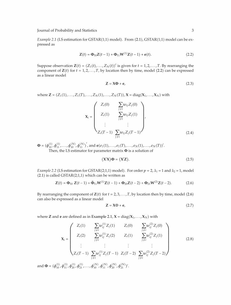
Example 2.1 (LS estimation for GSTAR(1;1)model). From (2.1), GSTAR(1;1)model can be ex-pressed as

Z(t) = Φ10Z(t − 1) +Φ11W(1)Z(t − 1) + e(t). (2.2)

Suppose observation Z(t) = (Z1(t), . . . , ZN(t))′ is given for t = 1, 2, . . . , T . By rearranging thecomponent of Z(t) for t = 1, 2, . . . , T , by location then by time, model (2.2) can be expressedas a linear model

Z = XΦ + e, (2.3)

where Z = (Z1(1), . . . , Z1(T), . . . , ZN(1), . . . , ZN(T)), X = diag(X1, . . . ,XN) with

Xi =

⎛⎜⎜⎜⎜⎜⎜⎜⎜⎝

Zi(0)∑

j /= i

wijZj(0)

Zi(1)∑

j /= i

wijZj(1)

......

Zi(T − 1)∑

j /= i

wijZj(T − 1)

⎞⎟⎟⎟⎟⎟⎟⎟⎟⎠

,

(2.4)

Φ = (φ(1)10 , φ

(1)11 , . . . , φ

(N)10 , φ

(N)11 )

′, and e(e1(1), . . . , e1(T), . . . , eN(1), . . . , eN(T))′.

Then, the LS estimator for parameter matrix Φ is a solution of(X′X

)Φ =

(X′Z

). (2.5)

Example 2.2 (LS estimation for GSTAR(2;1,1)model). For order p = 2, λ1 = 1 and λ2 = 1, model(2.1) is called GSTAR(2;1,1) which can be written as

Z(t) = Φ10 Z(t − 1) + Φ11W(1)Z(t − 1) +Φ20Z(t − 2) +Φ21W(2)Z(t − 2). (2.6)

By rearranging the component of Z(t) for t = 2, 3, . . . , T , by location then by time, model (2.6)can also be expressed as a linear model

Z = XΦ + e, (2.7)

where Z and e are defined as in Example 2.1, X = diag(X1, . . . ,XN) with

Xi =

⎛⎜⎜⎜⎜⎜⎜⎜⎜⎜⎝

Zi(1)∑

j /= i

w(1)ij Zj(1) Zi(0)

∑

j /= i

w(2)ij Zj(0)

Zi(2)∑

j /= i

w(1)ij Zj(2) Zi(1)

∑

j /= i

w(2)ij Zj(1)

......

......

Zi(T − 1)∑

j /= i

w(1)ij Zj(T − 1) Zi(T − 2)

∑

j /= i

w(2)ij Zj(T − 2)

⎞⎟⎟⎟⎟⎟⎟⎟⎟⎟⎠

(2.8)

and Φ = (φ(1)10 , φ

(1)11 , φ

(1)20 , φ

(1)21 , . . . , φ

(N)10 , φ

(N)11 , φ

(N)20 , φ

(N)21 )′.


Then, the LS estimator for parameter matrix Φ is a solution of(X′X

)Φ =

(X′Z

). (2.9)

3. Simulation Study

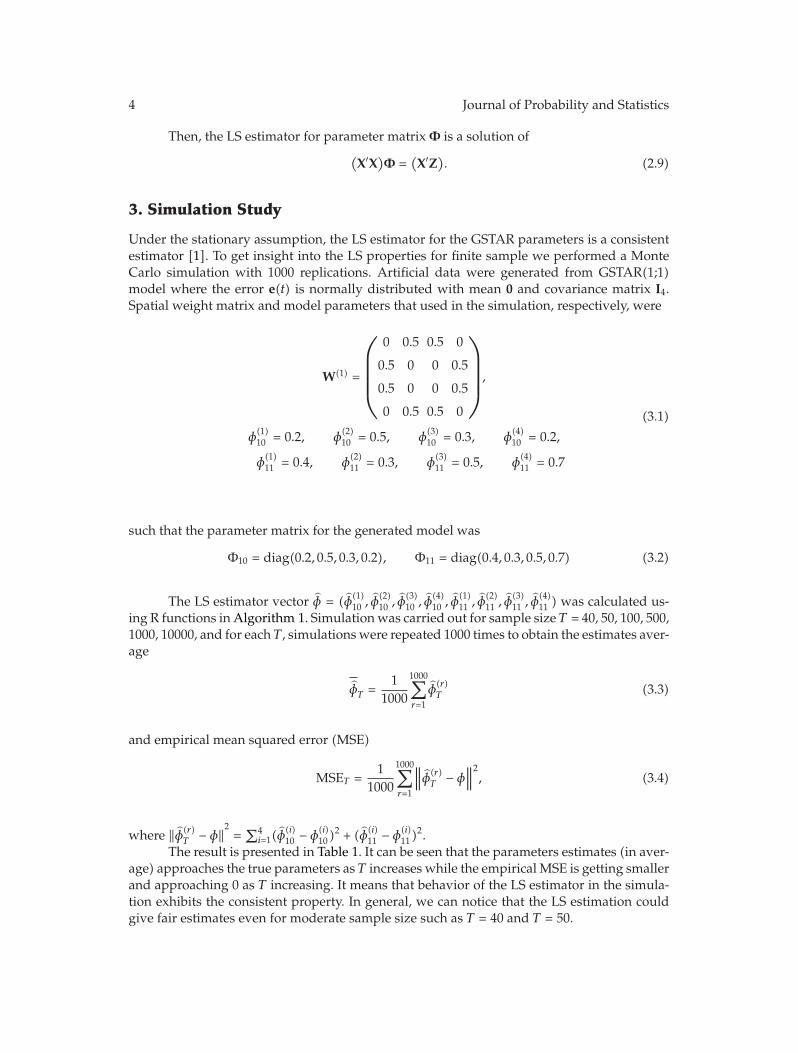
Under the stationary assumption, the LS estimator for the GSTAR parameters is a consistentestimator [1]. To get insight into the LS properties for finite sample we performed a MonteCarlo simulation with 1000 replications. Artificial data were generated from GSTAR(1;1)model where the error e(t) is normally distributed with mean 0 and covariance matrix I4.Spatial weight matrix and model parameters that used in the simulation, respectively, were

W(1) =

⎛⎜⎜⎜⎜⎜⎝

0 0.5 0.5 0

0.5 0 0 0.5

0.5 0 0 0.5

0 0.5 0.5 0

⎞⎟⎟⎟⎟⎟⎠

,

φ(1)10 = 0.2, φ

(2)10 = 0.5, φ

(3)10 = 0.3, φ

(4)10 = 0.2,

φ(1)11 = 0.4, φ

(2)11 = 0.3, φ

(3)11 = 0.5, φ

(4)11 = 0.7

(3.1)

such that the parameter matrix for the generated model was

Φ10 = diag(0.2, 0.5, 0.3, 0.2), Φ11 = diag(0.4, 0.3, 0.5, 0.7) (3.2)

The LS estimator vector φ = (φ(1)10 , φ

(2)10 , φ

(3)10 , φ

(4)10 , φ

(1)11 , φ

(2)11 , φ

(3)11 , φ

(4)11 ) was calculated us-

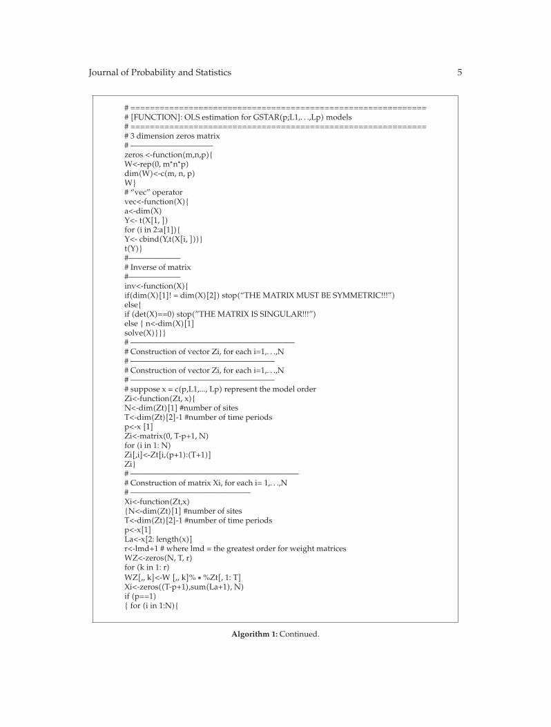
ing R functions in Algorithm 1. Simulationwas carried out for sample size T = 40, 50, 100, 500,1000, 10000, and for each T , simulations were repeated 1000 times to obtain the estimates aver-age

φT =1

1000

1000∑

r=1

φ(r)T (3.3)

and empirical mean squared error (MSE)

MSET =1

1000

1000∑

r=1

∥∥∥φ(r)T − φ

∥∥∥2, (3.4)

where ‖φ(r)T − φ‖2 = ∑4

i=1(φ(i)10 − φ

(i)10 )

2 + (φ(i)11 − φ

(i)11 )

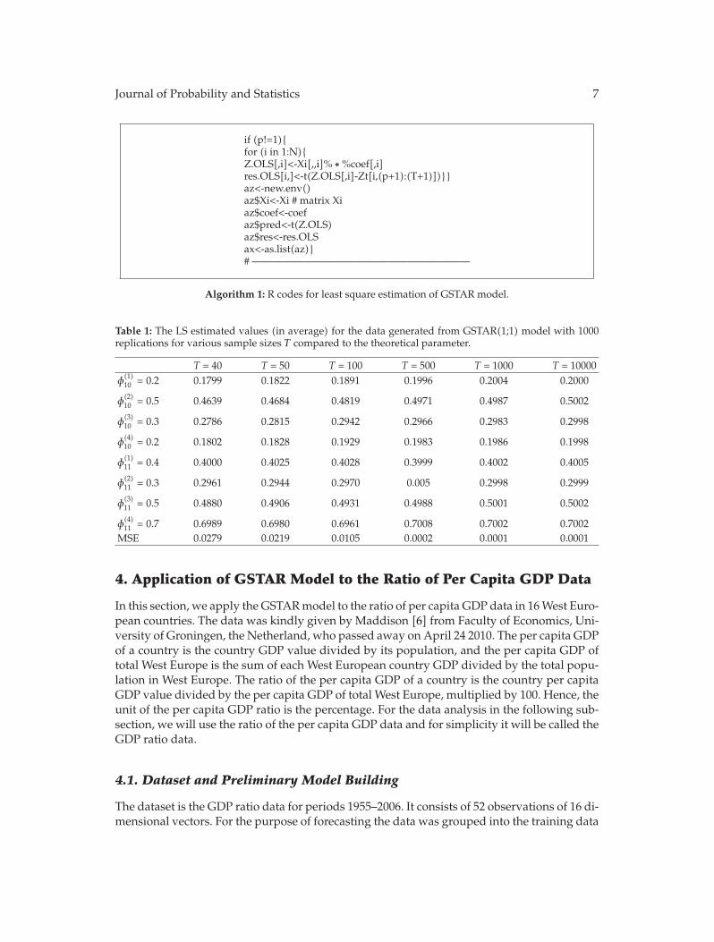
2.The result is presented in Table 1. It can be seen that the parameters estimates (in aver-

age) approaches the true parameters as T increases while the empirical MSE is getting smallerand approaching 0 as T increasing. It means that behavior of the LS estimator in the simula-tion exhibits the consistent property. In general, we can notice that the LS estimation couldgive fair estimates even for moderate sample size such as T = 40 and T = 50.


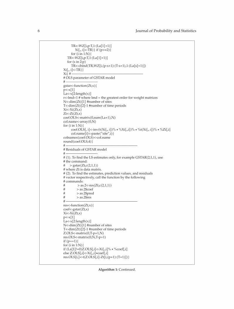
# =============================================================# [FUNCTION]: OLS estimation for GSTAR(p;L1,. . .,Lp) models# =============================================================# 3 dimension zeros matrix# ——————————-zeros <-function(m,n,p){W<-rep(0, m∗n∗p)dim(W)<-c(m, n, p)W}# “vec” operatorvec<-function(X){a<-dim(X)Y<- t(X[1, ])for (i in 2:a[1]){Y<- cbind(Y,t(X[i, ]))}t(Y)}#——————–# Inverse of matrix#——————–inv<-function(X){if(dim(X)[1]! = dim(X)[2]) stop(“THE MATRIX MUST BE SYMMETRIC!!!”)else{if (det(X)==0) stop(”THE MATRIX IS SINGULAR!!!”)else { n<-dim(X)[1]solve(X)}}}# ————————————————————–# Construction of vector Zi, for each i=1,. . .,N# ——————————————————# Construction of vector Zi, for each i=1,. . .,N# ——————————————————# suppose x = c(p,L1,..., Lp) represent the model orderZi<-function(Zt, x){N<-dim(Zt)[1] #number of sitesT<-dim(Zt)[2]-1 #number of time periodsp<-x [1]Zi<-matrix(0, T-p+1, N)for (i in 1: N)Zi[,i]<-Zt[i,(p+1):(T+1)]Zi}# —————————————————————# Construction of matrix Xi, for each i= 1,. . .,N# ———————————————Xi<-function(Zt,x){N<-dim(Zt)[1] #number of sitesT<-dim(Zt)[2]-1 #number of time periodsp<-x[1]La<-x[2: length(x)]r<-lmd+1 # where lmd = the greatest order for weight matricesWZ<-zeros(N, T, r)for (k in 1: r)WZ[,, k]<-W [,, k]% ∗%Zt[, 1: T]Xi<-zeros((T-p+1),sum(La+1), N)if (p==1){ for (i in 1:N){

Algorithm 1: Continued.


TR<-WZ[i,p:T,1:(La[1]+1)]Xi[,, i]<-TR}} if (p>=2){

for (i in 1:N){TR<-WZ[i,p:T,1:(La[1]+1)]for (s in 2:p)

TR<-cbind(TR,WZ[i,(p-s+1):(T-s+1),1:(La[s]+1)])Xi[,, i]<-TR}}Xi} # —————————————————————# OLS parameter of GSTAR model# —————————-gstar<-function(Zt,x){p<-x[1]La<-x[2:length(x)]r<-lmd+1 # where lmd = the greatest order for weight matricesN<-dim(Zt)[1] #number of sitesT<-dim(Zt)[2]-1 #number of time periodsXi<-Xi(Zt,x)Zi<-Zi(Zt,x)coef.OLS<-matrix(0,sum(La+1),N)col.name<-array(0,N)for (i in 1:N){

coef.OLS[, i]<-inv(t(Xi[,, i])% ∗%Xi[,,i])% ∗%t(Xi[,, i])% ∗%Zi[,i]col.name[i]<-paste(”site”,i)}

colnames(coef.OLS)<-col.nameround(coef.OLS,4)}# —————————————————————# Residuals of GSTAR model# —————————-# (1). To find the LS estimates only, for example GSTAR(2;1,1), use# the command:# > gstar(Zt,c(2,1,1))# where Zt is data matrix.# (2). To find the estimates, prediction values, and residuals# vector respectively, call the function by the following# commands:# > as.2<-res(Zt,c(2,1,1))# > as.2$coef# > as.2$pred# > as.2$res# —————————————————————res<-function(Zt,x){coef<-gstar(Zt,x)Xi<-Xi(Zt,x)p<-x[1]La<-x[2:length(x)]N<-dim(Zt)[1] #number of sitesT<-dim(Zt)[2]-1 #number of time periodsZ.OLS<-matrix(0,T-p+1,N)res.OLS<-matrix(0,N,T-p+1)if (p==1){for (i in 1:N){if (La[1]!=0)Z.OLS[,i]<-Xi[,,i]% ∗%coef[,i]else Z.OLS[,i]<-Xi[,,i]∗coef[,i]res.OLS[i,]<-t(Z.OLS[,i]-Zt[i,(p+1):(T+1)])}

Algorithm 1: Continued.


if (p!=1){for (i in 1:N){Z.OLS[,i]<-Xi[,,i]% ∗%coef[,i]res.OLS[i,]<-t(Z.OLS[,i]-Zt[i,(p+1):(T+1)])}}az<-new.env()az$Xi<-Xi # matrix Xiaz$coef<-coefaz$pred<-t(Z.OLS)az$res<-res.OLSax<-as.list(az)}# —————————————————————

Algorithm 1: R codes for least square estimation of GSTAR model.

Table 1: The LS estimated values (in average) for the data generated from GSTAR(1;1) model with 1000replications for various sample sizes T compared to the theoretical parameter.

T = 40 T = 50 T = 100 T = 500 T = 1000 T = 10000φ(1)10 = 0.2 0.1799 0.1822 0.1891 0.1996 0.2004 0.2000

φ(2)10 = 0.5 0.4639 0.4684 0.4819 0.4971 0.4987 0.5002

φ(3)10 = 0.3 0.2786 0.2815 0.2942 0.2966 0.2983 0.2998

φ(4)10 = 0.2 0.1802 0.1828 0.1929 0.1983 0.1986 0.1998

φ(1)11 = 0.4 0.4000 0.4025 0.4028 0.3999 0.4002 0.4005

φ(2)11 = 0.3 0.2961 0.2944 0.2970 0.005 0.2998 0.2999

φ(3)11 = 0.5 0.4880 0.4906 0.4931 0.4988 0.5001 0.5002

φ(4)11 = 0.7 0.6989 0.6980 0.6961 0.7008 0.7002 0.7002

MSE 0.0279 0.0219 0.0105 0.0002 0.0001 0.0001

4. Application of GSTAR Model to the Ratio of Per Capita GDP Data

In this section, we apply the GSTARmodel to the ratio of per capita GDP data in 16West Euro-pean countries. The data was kindly given by Maddison [6] from Faculty of Economics, Uni-versity of Groningen, the Netherland, who passed away on April 24 2010. The per capita GDPof a country is the country GDP value divided by its population, and the per capita GDP oftotal West Europe is the sum of each West European country GDP divided by the total popu-lation in West Europe. The ratio of the per capita GDP of a country is the country per capitaGDP value divided by the per capita GDP of total West Europe, multiplied by 100. Hence, theunit of the per capita GDP ratio is the percentage. For the data analysis in the following sub-section, we will use the ratio of the per capita GDP data and for simplicity it will be called theGDP ratio data.

4.1. Dataset and Preliminary Model Building

The dataset is the GDP ratio data for periods 1955–2006. It consists of 52 observations of 16 di-mensional vectors. For the purpose of forecasting the data was grouped into the training data


1960 1970 1980 1990 2000

50

100

150

200

Training data

Test data

(a)

1960 1970 1980 1990

5

10

−10

−5

0

(b)

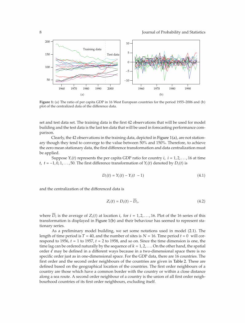
Figure 1: (a) The ratio of per capita GDP in 16 West European countries for the period 1955–2006 and (b)plot of the centralized data of the difference data.

set and test data set. The training data is the first 42 observations that will be used for modelbuilding and the test data is the last ten data that will be used in forecasting performance com-parison.

Clearly, the 42 observations in the training data, depicted in Figure 1(a), are not station-ary though they tend to converge to the value between 50% and 150%. Therefore, to achievethe zeromean stationary data, the first difference transformation and data centralizationmustbe applied.

Suppose Yi(t) represents the per capita GDP ratio for country i, i = 1, 2, . . . , 16 at timet, t = −1, 0, 1, . . . , 50. The first difference transformation of Yi(t) denoted by Di(t) is

Di(t) = Yi(t) − Yi(t − 1) (4.1)

and the centralization of the differenced data is

Zi(t) = Di(t) −Di, (4.2)

where Di is the average of Zi(t) at location i, for i = 1, 2, . . . , 16. Plot of the 16 series of thistransformation is displayed in Figure 1(b) and their behaviour has seemed to represent sta-tionary series.

As a preliminary model building, we set some notations used in model (2.1). Thelength of time period is T = 40, and the number of sites isN = 16. Time period t = 0 will cor-respond to 1956, t = 1 to 1957, t = 2 to 1958, and so on. Since the time dimension is one, thetime lag can be ordered naturally by the sequence of k = 1, 2, . . .. On the other hand, the spatialorder � may be defined in a different ways because in a two-dimensional space there is nospecific order just as in one-dimensional space. For the GDP data, there are 16 countries. Thefirst order and the second order neighbours of the countries are given in Table 2. These aredefined based on the geographical location of the countries. The first order neighbours of acountry are those which have a common border with the country or within a close distancealong a sea route. A second order neighbour of a country is the union of all first order neigh-bourhood countries of its first order neighbours, excluding itself.


Table 2: Geographical neighbourhood of order 1 and order 2.

No. Country Countries in the 1st neighborhood Countries in the 2nd neighborhood1 Austria 6,9,15 2,3,5,7,10,142 Belgium 5,6,10,16 1,3,8,9,13,14,153 Denmark 6,10,11,14 1,2,4,5,15,164 Finland 11,14 3,65 France 2,6,9,13,15,16 1,3,7,8,10,12,146 Germany 1,2,3,5,10,14,15 4,9,11,13,167 Greece 9 1,5,158 Ireland 16 2,5,109 Italy 1,5,7,15 2,6,13,1610 Netherland 2,3,6,16 1,5,8,11,14,1511 Norway 3,4,14 6,1012 Portugal 13 513 Spain 5,12 2,6,9,15,1614 Sweden 3,4,6,11 1,2,5,10,1515 Switzerland 1,5,6,9 2,3,7,10,13,14,1616 United Kingdom 2,5,8,10 3,6,9,13,15

Suppose n(�)i , � = 1, 2 represents the number of countries which are the �th neighbours

of a country i. The spatial weight of order � between countries i and j can be defined as

w(�)ij =

⎧⎪⎨

⎪⎩

1

n(�)i

, if j is the �th neighbours of i,

0, if j is not the �th neighbours of i.(4.3)

For example, from Table 2 it can be seen that Austria has 3 the first order neighbours, Ger-many, Netherland and Switzerland, and has 6 second order neighbours, Belgium, Denmark,France, Greece, Netherland, and Sweden. Then, the first order of spatial weight betweenAustria and each nearby country is

w(1)16 = w

(1)19 = w

(1)1,15 =

13

(4.4)

and the second order of spatial weight is w(2)12 = w

(2)13 = w

(2)15 = w

(2)17 = w

(2)1,10 = w

(2)1,14 = 1/6.

4.2. GSTAR Model Building for the GDP Data

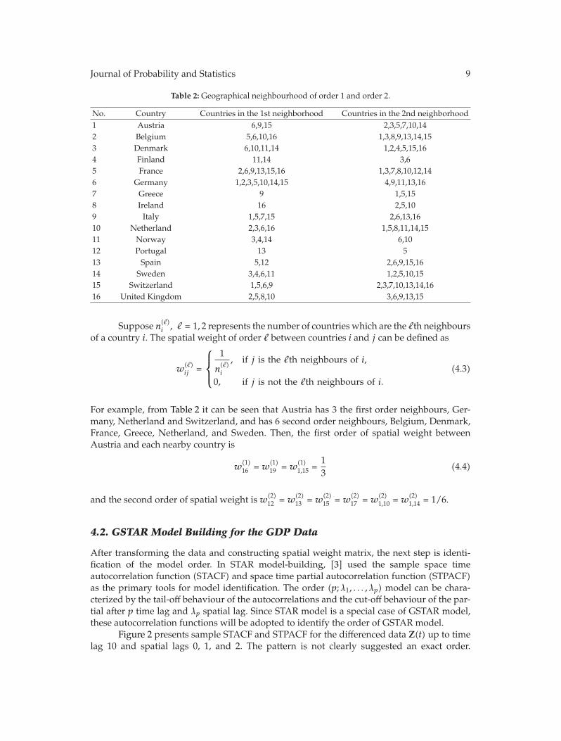
After transforming the data and constructing spatial weight matrix, the next step is identi-fication of the model order. In STAR model-building, [3] used the sample space timeautocorrelation function (STACF) and space time partial autocorrelation function (STPACF)as the primary tools for model identification. The order (p;λ1, . . . , λp) model can be chara-cterized by the tail-off behaviour of the autocorrelations and the cut-off behaviour of the par-tial after p time lag and λp spatial lag. Since STAR model is a special case of GSTAR model,these autocorrelation functions will be adopted to identify the order of GSTAR model.

Figure 2 presents sample STACF and STPACF for the differenced data Z(t) up to timelag 10 and spatial lags 0, 1, and 2. The pattern is not clearly suggested an exact order.


Aut

ocor

rela

tion

10

Time lag

2 4 6 8

STPACF at spatial lag 0 STPACF at spatial lag 1 STPACF at spatial lag 2

STACF at spatial lag 0 STACF at spatial lag 1 STACF at spatial lag 2

10

Time lag

2 4 6 8 10

Time lag

2 4 6 8

Part

ial

10

Time lag

2 4 6 8 10

Time lag

2 4 6 8 10

Time lag

2 4 6 8

Aut

ocor

rela

tion

Aut

ocor

rela

tion

Part

ial

Part

ial

0

0.20.1

−0.1−0.2

0

0.20.1

−0.1−0.2

0

0.20.1

−0.1−0.2

0

0.20.1

−0.1−0.2

0

0.20.1

−0.1−0.2

0

0.20.1

−0.1−0.2

Figure 2: Sample space-time ACF and PACF of the differenced data.


10

Time lag

2 4 6 8

Aut

ocor

rela

tion

10

Time lag

2 4 6 8 10

Time lag

2 4 6 8

Aut

ocor

rela

tion

Aut

ocor

rela

tion

0

0.20.1

−0.1−0.2

0

0.20.1

−0.1−0.2

0

0.20.1

−0.1−0.2

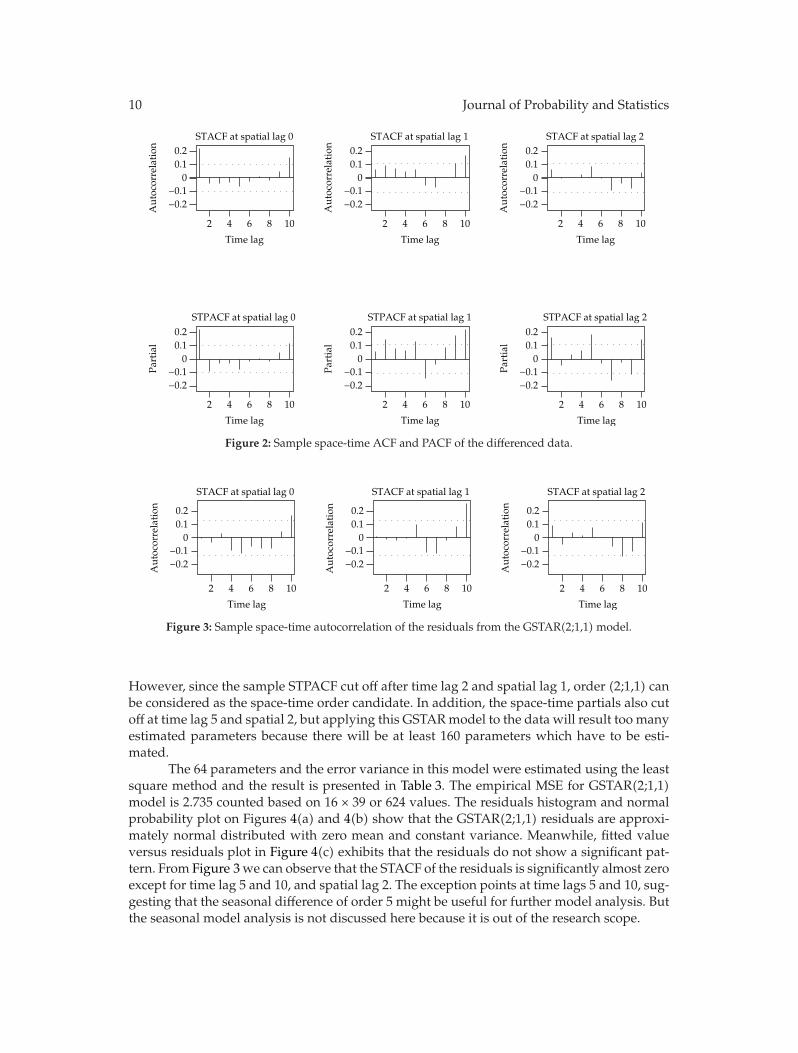
Figure 3: Sample space-time autocorrelation of the residuals from the GSTAR(2;1,1) model.

However, since the sample STPACF cut off after time lag 2 and spatial lag 1, order (2;1,1) canbe considered as the space-time order candidate. In addition, the space-time partials also cutoff at time lag 5 and spatial 2, but applying this GSTARmodel to the data will result too manyestimated parameters because there will be at least 160 parameters which have to be esti-mated.

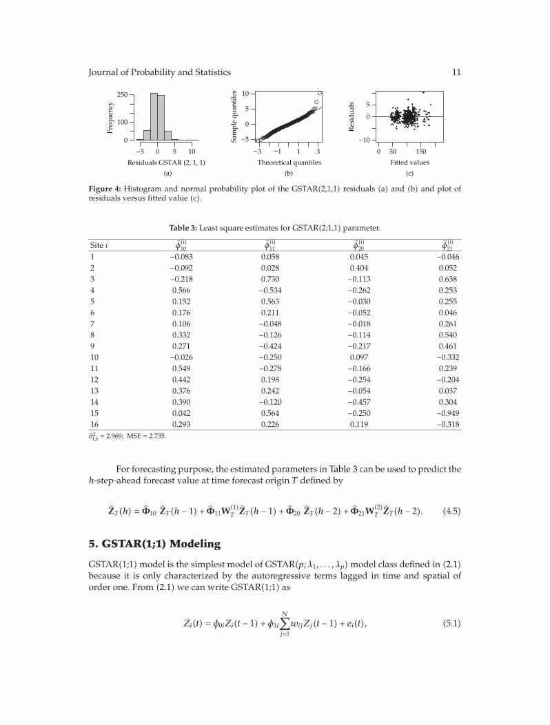
The 64 parameters and the error variance in this model were estimated using the leastsquare method and the result is presented in Table 3. The empirical MSE for GSTAR(2;1,1)model is 2.735 counted based on 16 × 39 or 624 values. The residuals histogram and normalprobability plot on Figures 4(a) and 4(b) show that the GSTAR(2;1,1) residuals are approxi-mately normal distributed with zero mean and constant variance. Meanwhile, fitted valueversus residuals plot in Figure 4(c) exhibits that the residuals do not show a significant pat-tern. From Figure 3 we can observe that the STACF of the residuals is significantly almost zeroexcept for time lag 5 and 10, and spatial lag 2. The exception points at time lags 5 and 10, sug-gesting that the seasonal difference of order 5 might be useful for further model analysis. Butthe seasonal model analysis is not discussed here because it is out of the research scope.


Residuals GSTAR (2, 1, 1)

(a)

Freq

uenc

y

5 10

0

100

250

1

10

Theoretical quantiles

(b)

Sam

ple

quan

tile

s

500 150

Fitted values

(c)

Res

idua

ls

−5 0

5

0

−5

3−3 −1

−10

5

0

Figure 4: Histogram and normal probability plot of the GSTAR(2,1,1) residuals (a) and (b) and plot ofresiduals versus fitted value (c).

Table 3: Least square estimates for GSTAR(2;1,1) parameter.

Site i φ(i)10 φ

(i)11 φ

(i)20 φ

(i)21

1 −0.083 0.058 0.045 −0.0462 −0.092 0.028 0.404 0.0523 −0.218 0.730 −0.113 0.6384 0.566 −0.534 −0.262 0.2535 0.152 0.563 −0.030 0.2556 0.176 0.211 −0.052 0.0467 0.106 −0.048 −0.018 0.2618 0.332 −0.126 −0.114 0.5409 0.271 −0.424 −0.217 0.46110 −0.026 −0.250 0.097 −0.33211 0.549 −0.278 −0.166 0.23912 0.442 0.198 −0.254 −0.20413 0.376 0.242 −0.054 0.03714 0.390 −0.120 −0.457 0.30415 0.042 0.564 −0.250 −0.94916 0.293 0.226 0.119 −0.318σ2LS = 2.969; MSE = 2.735.

For forecasting purpose, the estimated parameters in Table 3 can be used to predict theh-step-ahead forecast value at time forecast origin T defined by

ZT (h) = Φ10 ZT (h − 1) + Φ11W(1)T ZT (h − 1) + Φ20 ZT (h − 2) + Φ21W

(2)T ZT (h − 2). (4.5)

5. GSTAR(1;1) Modeling

GSTAR(1;1)model is the simplest model of GSTAR(p;λ1, . . . , λp)model class defined in (2.1)because it is only characterized by the autoregressive terms lagged in time and spatial oforder one. From (2.1) we can write GSTAR(1;1) as

Zi(t) = φ0iZi(t − 1) + φ1i

N∑

j=1

wijZj(t − 1) + ei(t), (5.1)


GSTAR (1;1) residuals

(a)

Freq

uenc

y

5

0

50

150

1

8

Theoretical quantiles

(b)

Sam

ple

quan

tile

s

500 150

Fitted values

(c)

Res

idua

ls

−5 0

4

0

−63−3 −1

−10

5

0

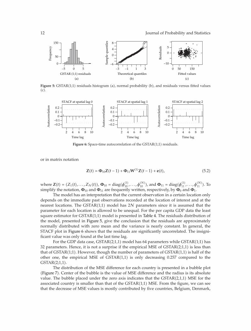
Figure 5: GSTAR(1;1) residuals histogram (a), normal probability (b), and residuals versus fitted values(c).


10

Time lag

2 4 6 8

Aut

ocor

rela

tion

10

Time lag

2 4 6 8 10

Time lag

2 4 6 8

Aut

ocor

rela

tion

Aut

ocor

rela

tion

0

0.20.1

−0.1−0.2

0

0.20.1

−0.1−0.2

0

0.20.1

−0.1−0.2

Figure 6: Space-time autocorrelation of the GSTAR(1;1) residuals.

or in matrix notation

Z(t) = Φ10Z(t − 1) +Φ11W(1)Z(t − 1) + e(t), (5.2)

where Z(t) = (Z1(t), . . . , ZN(t)), Φ10 = diag(φ(1)10 , . . . , φ

(N)10 ), and Φ11 = diag(φ(1)

11 , . . . , φ(N)11 ). To

simplify the notation, Φ10 and Φ11 are frequently written, respectively, by Φ0 and Φ1.The model has an interpretation that the current observation in a certain location only

depends on the immediate past observations recorded at the location of interest and at thenearest locations. The GSTAR(1;1) model has 2N parameters since it is assumed that theparameter for each location is allowed to be unequal. For the per capita GDP data the leastsquare estimator for GSTAR(1;1) model is presented in Table 4. The residuals distribution ofthe model, presented in Figure 5, give the conclusion that the residuals are approximatelynormally distributed with zero mean and the variance is nearly constant. In general, theSTACF plot in Figure 6 shows that the residuals are significantly uncorrelated. The insigni-ficant value was only found at the last time lag.

For the GDP data case, GSTAR(2;1,1) model has 64 parameters while GSTAR(1;1) has32 parameters. Hence, it is not a surprise if the empirical MSE of GSTAR(2;1,1) is less thanthat of GSTAR(1;1). However, though the number of parameters of GSTAR(1,1) is half of theother one, the empirical MSE of GSTAR(1,1) is only decreasing 0.257 compared to theGSTAR(2;1,1).

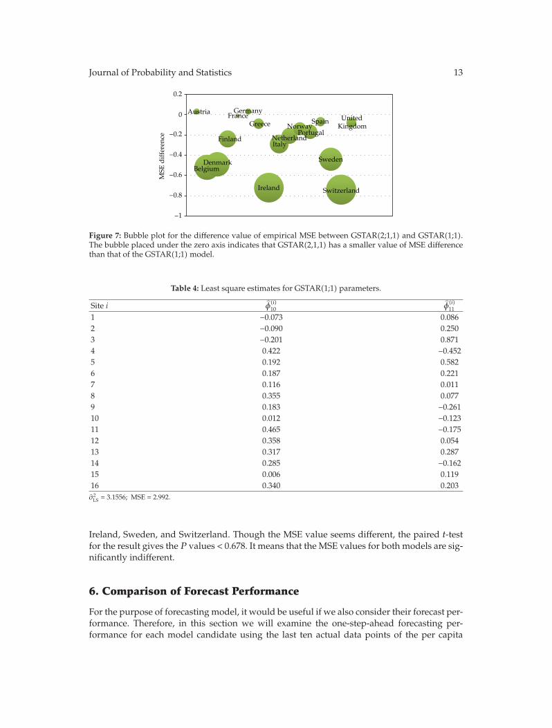
The distribution of the MSE difference for each country is presented in a bubble plot(Figure 7). Center of the bubble is the value of MSE difference and the radius is its absolutevalue. The bubble placed under the zero axis indicates that the GSTAR(2,1,1) MSE for theassociated country is smaller than that of the GSTAR(1;1) MSE. From the figure, we can seethat the decrease of MSE values is mostly contributed by five countries, Belgium, Denmark,


Austria

BelgiumDenmark

Finland

FranceGermany

Greece

Ireland

ItalyNetherland

NorwayPortugal

Spain

Sweden

Switzerland

United Kingdom

MSE

dif

fere

nce

0.2

0

−0.4

−1

−0.2

−0.6

−0.8

Figure 7: Bubble plot for the difference value of empirical MSE between GSTAR(2;1,1) and GSTAR(1;1).The bubble placed under the zero axis indicates that GSTAR(2,1,1) has a smaller value of MSE differencethan that of the GSTAR(1;1) model.

Table 4: Least square estimates for GSTAR(1;1) parameters.

Site i φ(i)10 φ

(i)11

1 −0.073 0.0862 −0.090 0.2503 −0.201 0.8714 0.422 −0.4525 0.192 0.5826 0.187 0.2217 0.116 0.0118 0.355 0.0779 0.183 −0.26110 0.012 −0.12311 0.465 −0.17512 0.358 0.05413 0.317 0.28714 0.285 −0.16215 0.006 0.11916 0.340 0.203σ2LS = 3.1556; MSE = 2.992.

Ireland, Sweden, and Switzerland. Though the MSE value seems different, the paired t-testfor the result gives the P values < 0.678. It means that the MSE values for both models are sig-nificantly indifferent.

6. Comparison of Forecast Performance

For the purpose of forecasting model, it would be useful if we also consider their forecast per-formance. Therefore, in this section we will examine the one-step-ahead forecasting per-formance for each model candidate using the last ten actual data points of the per capita


GDP ratio data set. Result of this section is expected to become a supplementary reference infinding the most parsimony space-time model for the case of per capita GDP ratio.

In (4.5) we have defined the h-step-ahead forecasting for GSTAR(2;1,1) model. ForGSTAR(1;1) model, it can be estimated by

ZT (h) = Φ10ZT (h − 1) +Φ11W(1)ZT (h − 1), (6.1)

ZT (h) = 0.1674 ZT (h − 1) + 0.0453W(1)ZT (h − 1), (6.2)

where Φ10 = diag(φ(1)10 , . . . , φ

(N)10 ),Φ11 = diag(φ(1)

11 , . . . , φ(N)11 ) , and for h ≤ 0, ZT (h) = Z(T − h).

The one-step-ahead forecast ZT+j−1(1) of each data points can be calculated using(4.5), (6.1), and (6.2) for h = 1. Note that calculation of the forecast value for each timej = 1, 2, . . . , 10, is performed without updating the parameter estimates and average data. Theone-step-ahead forecast for GSTAR(2;1,1) model is

ZT+j−1(1) = Φ10Z(T + j − 1

)+Φ11W(1)Z

(T + j − 1

)+Φ20Z

(T + j − 2

)

+Φ12W(1)Z(T + j − 1

),

(6.3)

where j = 1, 2, . . . , 10. Meanwhile the one-step-ahead forecast for GSTAR(1;1) model is

ZT+j−1(1) = Φ10Z(T + j − 1

)+Φ11W(1)Z

(T + j − 1

). (6.4)

To compare the forecast performance, we use mean of square forecast error (MSFE)which is defined by

MSFE =1N

N∑

i=1

Ei, (6.5)

where

Ei =110

10∑

j=1

[Yi

(T + j

) − Yi,T+j−1(1)]2,

Yi,T+j−1(1) =(Zi,T+j−1(1) +Di

)+ Yi

(T + j − 1

),

(6.6)

and Zi,T+j−1(1) is the element of Zi,T+j−1(1).To measure the performance closeness between two models, we also calculate the

MSFE difference between model M1 and model M2 for country i which is defined by

Ci = Ei(M1) − Ei(M2). (6.7)

The performance of M1 and M2 model is said to be close if the value of Ci is near tozero. The negative value of Ci indicates that for location i, the M1 model is better than M2


AustriaBelgium

DenmarkFinland

FranceGermany

Greece

Ireland

ItalyNetherland

Norway

PortugalSpain

Sweden

Switzerland

United Kingdom

0

1

2

3

MSF

E d

iffe

renc

e−2

−3

−4

−5

−1

Figure 8: Bubble plot for the difference of mean of square forecast error (MSFE) between GSTAR(2;1,1)and GSTAR(1;1). The bubble under the zero axis indicates that the GSTAR(2,1,1) has a smaller value ofMSFE difference than that of the GSTAR(1;1) model.

SFE

D

Site

1

Site

2

Site

3

Site

4

Site

5

Site

6

Site

7

Site

8

Site

9

Site

10

Site

11

Site

12

Site

13

Site

14

Site

15

Site

16

15

−5

5

−15

Figure 9: Square forecast error difference (SFED) for GSTAR(2;1,1) and GSTAR(1;1).

model. Since the residual is approximately normally distributed, the paired t-test can also beapplied to test the null hypothesis that modelM1 and modelM2 have the same forecast per-formance.

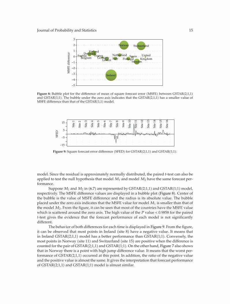
SupposeM1 andM2 in (6.7) are represented by GSTAR(2;1,1) and GSTAR(1;1)model,respectively. The MSFE difference values are displayed in a bubble plot (Figure 8). Center ofthe bubble is the value of MSFE difference and the radius is its absolute value. The bubbleplaced under the zero axis indicates that the MSFE value for modelM1 is smaller than that ofthe modelM2. From the figure, it can be seen that most of the countries have the MSFE valuewhich is scattered around the zero axis. The high value of the P value < 0.9858 for the pairedt-test gives the evidence that the forecast performance of each model is not significantlydifferent.

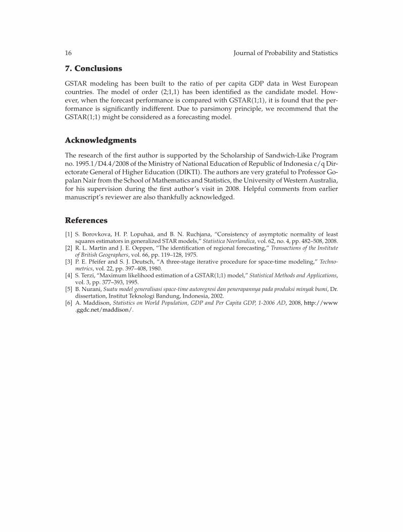
The behavior of both differences for each time is displayed in Figure 9. From the figure,it can be observed that most points in Ireland (site 8) have a negative value. It means thatin Ireland GSTAR(2;1,1) model has a better performance than GSTAR(1;1). Conversely, themost points in Norway (site 11) and Switzerland (site 15) are positive when the difference iscounted for the pair of GSTAR(2;1,1) andGSTAR(1;1). On the other hand, Figure 7 also showsthat in Norway there is a point with high jump difference value. It means that the worst per-formance of GSTAR(2;1,1) occurred at this point. In addition, the ratio of the negative valueand the positive value is almost the same. It gives the interpretation that forecast performanceof GSTAR(2;1,1) and GSTAR(1;1) model is almost similar.


7. Conclusions

GSTAR modeling has been built to the ratio of per capita GDP data in West Europeancountries. The model of order (2;1,1) has been identified as the candidate model. How-ever, when the forecast performance is compared with GSTAR(1;1), it is found that the per-formance is significantly indifferent. Due to parsimony principle, we recommend that theGSTAR(1;1) might be considered as a forecasting model.

Acknowledgments

The research of the first author is supported by the Scholarship of Sandwich-Like Programno. 1995.1/D4.4/2008 of theMinistry of National Education of Republic of Indonesia c/q Dir-ectorate General of Higher Education (DIKTI). The authors are very grateful to Professor Go-palanNair from the School ofMathematics and Statistics, the University ofWestern Australia,for his supervision during the first author’s visit in 2008. Helpful comments from earliermanuscript’s reviewer are also thankfully acknowledged.

References

[1] S. Borovkova, H. P. Lopuhaa, and B. N. Ruchjana, “Consistency of asymptotic normality of leastsquares estimators in generalized STARmodels,” Statistica Neerlandica, vol. 62, no. 4, pp. 482–508, 2008.

[2] R. L. Martin and J. E. Oeppen, “The identification of regional forecasting,” Transactions of the Instituteof British Geographers, vol. 66, pp. 119–128, 1975.

[3] P. E. Pfeifer and S. J. Deutsch, “A three-stage iterative procedure for space-time modeling,” Techno-metrics, vol. 22, pp. 397–408, 1980.

[4] S. Terzi, “Maximum likelihood estimation of a GSTAR(1;1)model,” Statistical Methods and Applications,vol. 3, pp. 377–393, 1995.

[5] B. Nurani, Suatu model generalisasi space-time autoregresi dan penerapannya pada produksi minyak bumi, Dr.dissertation, Institut Teknologi Bandung, Indonesia, 2002.

[6] A. Maddison, Statistics on World Population, GDP and Per Capita GDP, 1-2006 AD, 2008, http://www.ggdc.net/maddison/.

Submit your manuscripts athttp://www.hindawi.com

Hindawi Publishing Corporationhttp://www.hindawi.com Volume 2014

MathematicsJournal of


Mathematical Problems in Engineering

Hindawi Publishing Corporationhttp://www.hindawi.com

Differential EquationsInternational Journal of

Volume 2014

Applied MathematicsJournal of


Probability and StatisticsHindawi Publishing Corporationhttp://www.hindawi.com Volume 2014

Journal of


Mathematical PhysicsAdvances in

Complex AnalysisJournal of


OptimizationJournal of


CombinatoricsHindawi Publishing Corporationhttp://www.hindawi.com Volume 2014

International Journal of


Operations ResearchAdvances in

Journal of


Function Spaces

Abstract and Applied AnalysisHindawi Publishing Corporationhttp://www.hindawi.com Volume 2014

International Journal of Mathematics and Mathematical Sciences


The Scientific World JournalHindawi Publishing Corporation http://www.hindawi.com Volume 2014


Algebra

Discrete Dynamics in Nature and Society



Decision SciencesAdvances in

Discrete MathematicsJournal of

Hindawi Publishing Corporationhttp://www.hindawi.com

Volume 2014


Stochastic AnalysisInternational Journal of

Documents

Application of Generalized Space-Time Autoregressive Model on