Application of fuzzy minimum cost flow problems to network design under uncertainty

Fuzzy Sets and Systems 160 (2009) 3263–3289www.elsevier.com/locate/fss

Application of fuzzy minimum cost flow problems to networkdesign under uncertainty�

Mehdi Ghateea,b,∗, S. Mehdi Hashemia,b

aDepartment of Computer Science, Amirkabir University of Technology, No. 424, Hafez Avenue, Tehran 15875-4413, IranbLaboratory of Network and Optimization Research Center, Amirkabir University of Technology, Tehran, Iran

Received 21 April 2008; received in revised form 6 April 2009; accepted 13 April 2009Available online 24 April 2009

Abstract

This paper deals with fuzzy quantities and relations in multi-objective minimum cost flow problem. When t-norms and t-conormsare available, the goal programming is applied tominimize the deviation among themultiple costs of fuzzy flows and the given targetswhen the fuzzy supplies and demands are satisfied. To obtain the most optimistic and the most pessimistic satisficing solutions of thisproblem, two polynomial time algorithms are introduced applying some network transformations. To demonstrate the performanceof this approach in actual substances, network design under fuzziness is considered and an efficient scheme is proposed includinggenetic algorithm together with fuzzy minimum cost flow problem. This scheme is applied on a pilot network for more description.© 2009 Elsevier B.V. All rights reserved.

Keywords: Fuzzy network design; Fuzzy relations; Optimistic and pessimistic attitudes

1. Introduction

Network flow models provide a rich and powerful framework to formulate and solve many engineering and man-agement problems. A variety of applications, including the analysis and design of computer networks, cable televisionnetworks, transportation systems, communication networks, project schedules, queuing systems, inventory systems,and manpower allocation have been reported in the literature [2,28]. The minimum cost flow problem (MCFP) is a gen-eral structure in these models which provides a unified approach to many applications. This paper studies uncertaintyand impreciseness, multiple objectives and optimistic and pessimistic attitudes, dealing with a traditional minimum costflow problem and its application in network design. This problem is a reasonable generalization of fuzzy transportationproblem which was introduced by many researchers, see e.g., [32,43,21,25, 7,39,27,1,26,8].

� The authors were partially supported by Road Maintenance and Transportation Organization, Ministry of Roads and Transportation of Iran.∗Corresponding author at: Department of Computer Science, Amirkabir University of Technology, No. 424, Hafez Avenue, Tehran 15875-4413,

Iran. Tel.: +982164542522; fax: +982166497930.E-mail address: [email protected] (M. Ghatee).URL: http://math-cs.aut.ac.ir/∼ghatee (M. Ghatee).

0165-0114/$ - see front matter © 2009 Elsevier B.V. All rights reserved.doi:10.1016/j.fss.2009.04.004

http://www.elsevier.com/locate/fss

mailto:[email protected]

http://math-cs.aut.ac.ir/~ghatee

3264 M. Ghatee, S.M. Hashemi / Fuzzy Sets and Systems 160 (2009) 3263–3289

1.1. Uncertainty and impreciseness

Actual problems include uncertain data. Ramik [36] discussed on the origin of uncertainty and mentioned to theerrors in measuring physical quantities and representing the data in a computer. Uncertainty can be captured applyingfuzzy quantities. Keeping a fuzzy optimization problem in mind, one can apply satisficing approach in which thefuzzy target values are used in order to evaluate solutions absolutely [20,3]. Applying the possibility and the necessitymeasures [10], the traditional optimal solution set is extended to a pair of fuzzy sets, namely, the possibly optimal andthe necessarily optimal solution sets [41,42]. Inuiguchi and Sakawa [18] considered different extensions of relationsutilizing t-norms and t-conorms treating with fuzzy linear programming. Some extensions of satisficing approach havebeen presented in [19]. It is also demonstrated that the different combination of possibility and necessitymeasures yieldsvarious solutions depending on the decision maker’s intention [10,20,19,36]. To see the application of this approach incellular manufacturing systems, we refer to [37].

1.2. Multiple objectives

Multi-objective models have crucial role in the mathematical programming and applications [17,24,30]. For exam-ple, Kothari and Dhillon [23] collected some industrial applications of this viewpoint in power system optimizationand Brar et al. [5] investigated fuzzy multiple objectives in this problem. An important approach dealing with suchproblems is the goal programming in which the deviation between each objective function and its target value should beminimized [16]. The linguistic statements as target values are qualified byRamik [33] elicitingmembership functions offuzzy sets.

1.3. Optimistic and pessimistic attitudes

In the fuzzy linear programming, the necessity and the possibility measures are used to evaluate to what extent itis necessary and it is possible that a solution satisfies a constraint, respectively. Analogues, a feasible and optimalsolution for at least one real scenario with membership degree not less than h is called a �-possibly optimal solution. An�-necessarily optimal solution is a feasible and optimal solution of any real scenario with membership degree more than1− �. Julien [22] transformed the fuzzy linear programming problem with the best and the worst linear programmingproblems at different �-cuts and Liu [29] measured the fulfillment of the constraints when the constraints are tight orloose based on own pessimistic or optimistic attitudes.

1.4. MCFP related works

Multi-objective MCFP has been significantly studied in the literature [15]. Fuzzy multi-level MCFP with fuzzycosts was also introduced by Shih and Lee considering different certainty degrees and applying linear programmingalgorithms. Liu and Kao [28] solved MCFP with fuzzy costs using Yager’s ranking function which maintains thenetwork structure of the problem which permits to use network simplex method. Ghatee and Hashemi [13] presentedsome different cases of fuzzy MCFP utilizing a total order and nominal flows. Then, the authors in [12] investigatedfully fuzzified MCFP considering a large variety of ranking functions. Duality concepts were addressed in [14], too.The application of fuzzy MCFP in internet transmission [28], petroleum industry [12] and bus network planning [13],have been also presented in recent literature.

1.5. The contribution of the present paper

This paper treats with a multi-objective fully fuzzified MCFP with fuzzy quantities and fuzzy relations. Consideringfuzzy goals, the satisficing approach is pursued. Taking this scheme in mind, the solution of how many units shouldbe transported between each pair of supplier and demander nodes, may be obtained in which the amount of supplies,demands and transportation costs are exhibited with fuzzy numbers. Then the application of this scheme in networkdesign under fuzziness is discussed. For this aim a genetic algorithmwhose utility function is evaluated by the proposedalgorithms is implemented. On a real network this idea is illustrated. The rest of paper is organized as follows.Some basic definitions are given in next section. In Section 3, the fully fuzzified multi-objective MCFP is discussed.

M. Ghatee, S.M. Hashemi / Fuzzy Sets and Systems 160 (2009) 3263–3289 3265

The optimistic and pessimistic satisficing flows are introduced in Sections 4 and 5, respectively. Fuzzy network designand numerical experiments are presented in Section 6. The last section ends this paper with a brief conclusion andfuture directions.

2. Fuzzy sets and relations

The class of fuzzy sets on X is denoted with F(X ). Let a ∈ F(X ) with membership function �a(x), for each x ∈ X .The �-cut or �-level of a is defined as an ordinary set [a]� whose members satisfy �a(x)� 0, see [6]. The supportand the height are given by Supp(a) = closure{x ∈ X |�a(x) > 0} and Hgt(a) = {x ∈ X |�a(x) = 1}, respectively.Each element of Supp(a) is said a realization or a scenario. a ∈ a means that a ∈ Supp(a) or equivalently �a(a) > 0.When A is a fuzzy matrix including fuzzy sets as elements, A ∈ A implies that each element of A belongs to thecorresponding element of A. a ∈ F(R) is a fuzzy number when a is a convex normalized fuzzy set whose membershipfunction is piecewise continuous. It is well defined denoting the �-level set of a fuzzy number a with a closed interval[aL (�), aR(�)]. In what follows, we focus on triangular norms whose best results have been introduced by Dubois andPrade [9], Ramik [33,35,36], Ramik and Vlach [34] and Inuiguchi et al. [19].

Definition 2.1. Let T : [0, 1]2 −→ [0, 1] and S : [0, 1]2 −→ [0, 1] are commutative, associative, non-decreasing inevery variable and satisfy the following boundary conditions:

T (a, 1) = a for all a ∈ [0, 1],

S(a, 0) = a for all a ∈ [0, 1].

Then T and S are called the triangular norm (t-norm) and triangular conorm (t-conorm), respectively.

Definition 2.2. Let ai belongs to [0, 1] for i = 1, . . . , n. When m ∈ {1, . . . , n}, one can denote T1,. . .,m, T

i∈{1,. . .,m} orT (ai |i ∈ {1, . . . ,m}) for the following induction definition:

T1,2 = T (a1, a2),

and for m > 2,

T1,. . .,m = T (T

1,. . .,(m−1), am).

A particular fuzzy extension of relation P is often denoted by tilde, i.e., P . When t-norm T or t-conorm S is used toextend a particular fuzzy set a, the membership function is denoted with �aT or �aS , respectively.

Definition 2.3 (Ramik [33]). Let X, Y be non-empty sets, T and S be a t-norm and t-conorm, respectively. Let P be abinary relation on X × Y . Then, two fuzzy extended relations PT and PS may be defined for all fuzzy sets a, b, thata ∈ F(X ) and b ∈ F(Y ) with the following membership functions, respectively,

�PT (a, b) = sup{T (�P (x, y), T (�a(x), �b(y)))|x ∈ a, y ∈ b},�PS (a, b) = inf{S(�P (x, y), S(1 − �a(x), 1 − �b(y)))|x ∈ a, y ∈ b},

where sup(�) = 0 and inf(�) = 1.

CommonlyPos(a � b) = �� T (a, b) andNes(a � b) = � � S

(a, b) are referred to possibility and necessity measures.Note that Pos(a � b) evaluates to what extent it is possible that the variable a is in the fuzzy set b. On the other hand,Nes(a � b) evaluates to what extent it is certain that the variable a is in the fuzzy set b. Also, a �

T b and a � Sb implythat a is less than b with possibility degree �

� T (a, b) and necessity degree � � S(a, b), respectively. In fact, if one says

x is a possible solution for a fuzzy programming problem with positive membership value �, it means that x is optimalfor at least one realization of this fuzzy programming problem with a certainty degree greater than �. On the otherhand, a necessary solution of fuzzy programming problem with positive membership value � is an optimal solution forall of the realizations whose membership degrees are greater than 1 − �, see [18].


Proposition 2.4 (Inuiguchi et al. [19]). Let a, b ∈ F(X ) be normal and compact fuzzy sets, with T = min, S = maxand � ∈ (0, 1), we have,

(i) �� T (a, b)� � ⇔ inf [a]� � sup[b]�,

(ii) � � S(a, b)� � ⇔ sup[a]1−� � inf [b]1−�,

(iii) �� T (a, b)� � ⇔ sup[a]� � inf [b]�,

(iv) � � S(a, b)� � ⇔ inf [a]1−� � sup[b]1−�.

3. Fully fuzzified multi-objective MCFP

MCFP arises naturally in engineering and economics contexts; it appears in problems involving equilibrium modelssuch as urban transportation systems [40], resistive electrical networks [23] designing and production–distributionproblems [2]. The central concept in all of these problems is to find the least transportation cost of a commoditythrough a capacitated network in order to satisfy demands at certain nodes using available supplies at other nodes. LetG = (N , A) be a directed network where N and A denote sets of nodes and links, respectively. For each link (i, j) ∈ A,

multiple costs cki, j , k = 1, . . . , K , an upper bound capacity ui, j and a lower bound capacity li, j are considered.The multiple costs including e.g., the economic, the shortness, the environmental and the security indices may besimultaneously considered in engineering problems [23,5]. Assume li, j = 0. Multi-objective MCFP requirements canbe expressed as follows when the network is bipartite:

min f k(y) =K∑

k=1

∑(i, j)∈A

cki, j ui, j yi, j (1)

s.t. ⎧⎪⎪⎪⎪⎨⎪⎪⎪⎪⎩

(a)∑

{ j :(i, j)∈A}ui, j yi, j � si , i ∈ S,

(b)∑

{ j :( j,i)∈A}u j,i y j,i � di , i ∈ D,

(c) 0� yi, j � 1,

(2)

where yi, j is the rate of usage of link (i, j) ∈ A and xi, j = yi, j ui, j is the corresponding flow through link (i, j).S andD are the sets of supplier and demander nodes. Eq. (2a) ensures that the output of supplier node i is at most si , andEq. (2b) implies that the input to demander node i ∈ D is at least di . It seems that this formulation is different fromtraditional MCFP formulation [2,28,38,12]; however, the following shows the equivalency.

Remark 3.1. The optimization problem (1) subject to (2) can be transformed into the following traditional multi-objective MCFP:

min f k(y) =K∑

k=1

∑(i, j)∈A

cki, j xi, j (3)

s.t. ∑{ j :(i, j)∈A}

xi, j −∑

{ j :( j,i)∈A}x j,i = bi , ∀i ∈ N , 0� xi, j � ui, j , ∀(i, j) ∈ A. (4)

The converse statement is also true.

Proof. Consider a new node p which can play the role of an inventory or a dummy customer which is dependent onthe greatness of

∑i∈S si and

∑i∈D di . When

∑i∈S si �

∑i∈D di , node p is a dummy costumer otherwise p is an


inventory node. Then (2a) and (2b) can be rewritten as⎧⎪⎨⎪⎩(a′)

∑{ j :(i, j)∈A}

xi, j + xi,p = si , i ∈ S,

(b′) − ∑{ j :( j,i)∈A}

x j,i − xp,i = −di , i ∈ D.(5)

For node p one can write

∑{ j :(p, j)∈A}

xp, j −∑

{ j :( j,i)∈A}x j,p = −

⎛⎝∑

i∈Ssi −

∑i∈D

di

⎞⎠ . (6)

Thus, connecting each node i ∈ S to node p with link (i, p) and node p to node i ∈ D with link (p, i) producesa network with balance flow constraints analogues to (4) in which a new (n + 1)-vector b is defined that for eachi ∈ S (i ∈ D), bi = si (bi = −di ) and bi = 0 otherwise. Also set bn+1�bp = −(

∑i∈S si −

∑i∈D di ). To ensure that

such dummy links are chosen when there is no other possibility, the cost, also, the capacity of such links are assumedto be sufficiently large. As a simple exercise, it is possible to show that each feasible solution of the original problemis feasible for this model and conversely. �

When one treats with problem (3) subjected to (4), it is possible to define another equivalent bipartite network. Forthis aim all of the supplier nodes are included in S and the demander nodes are included in D. Other nodes can beaugmented to S or D arbitrary whose supplies and demands are zero. Now define

S′ = { i ′ |i ∈ S ∪D},D′ = { i ′′ |i ∈ S ∪D},A′ = { (i ′, i ′′) | i ′ ∈ S′ & i ′′ ∈ D′} ∪ {(i ′, j ′′) | (i, j) ∈ A}.

For each link (i ′, i ′′) the cost and upper bound capacity are defined as zero and infinity, respectively. Also for each link(i ′, j ′′) the cost and the upper bound capacity are equal to ci, j and ui, j , respectively. Let Q be the sum of supplies orthe sum of demands. For each node i ∈ S set si ′ = si + Q and si ′′ = Q. For each node i ∈ D set di ′′ = di + Qand di ′ = Q. Applying these modifications, the network depicted in Fig. 2c is a transformed network of the networkof Fig. 2a. The interested reader can show the equivalency of the results of flow transmission through both of thenetworks.In what follows, we investigate a more reasonable variant of this transportation problems in which the links costs,

the nodes supplies and the node demands are not precisely known. Due to granular information about human, social,economic, and political interactions, the expert system may state the following fully fuzzified multi-objective MCFPcapturing with uncertainty:

min f k(y) =∑

(i, j)∈A

cki, j ui, j yi, j , ∀k = 1, . . . , K (7)

s.t. ⎧⎪⎪⎪⎪⎪⎪⎪⎪⎨⎪⎪⎪⎪⎪⎪⎪⎪⎩

gs,i (y) = ∑{ j :(i, j)∈A}

ui, j yi, j � si , i ∈ S,

gd,i (y) = ∑{ j :( j,i)∈A}

u j,i y j,i � di , i ∈ D,

∑{ j :(i, j)∈A}

ui, j .yi, j = ∑{ j :( j,i)∈A}

u j,i .y j,i , i ∈ N\(S ∪D),

0� yi, j � 1,

(8)

where cki, j , ui, j , si and di are fuzzy numbers. Note that this problem is a special variant of fuzzy linear programmingwhich was introduced e.g., by Inuiguchi et al. [19] and Ramik [31,33,36].


Analogues to the crisp case, the fuzzy flow is defined as xi, j = ui, j yi, j . Hereafter, for notation convenience denote�ki, j�cki, j ui, j . A matrix y = (yi, j ) ∈ [0, 1]n×n such that

∑{ j :(i, j)∈A} xi, j = ∑

{ j :(i, j)∈A} ui, j yi, j = ∑{ j :( j,i)∈A} u j,i

y j,i = ∑{ j :( j,i)∈A} x j,i for all i ∈ N\(S ∪D) is said a semi-feasible rate matrix. YSF is a set including semi-feasible

rate matrices.Since, f k(y) for k = 1, . . . , K , gs,i (y) for i ∈ S and gd,i (y) for i ∈ D are parametric fuzzy sets with respect to

crisp vector y ∈ YSF , their membership functions may be stated as below using t-norm T,

�f k (y)

T (z) = sup

⎧⎨⎩T (��ki, j

(�ki, j )|(i, j) ∈ A) |�k ∈ �k, y ∈ YSF ,∑

(i, j)∈A

�ki, j yi, j = z

⎫⎬⎭ , (9)

�gs,i (y)T(s) = sup

⎧⎨⎩T (�ui, j (ui, j )|(i, j) ∈ A) | u ∈ u, y ∈ YSF ,

∑(i, j)∈A

ui, j yi, j = s

⎫⎬⎭ , (10)

�gd,i (y)T(d) = sup

⎧⎨⎩T (�u j,i

(u j,i )|( j, i) ∈ A) | u ∈ u, y ∈ YSF ,∑

( j,i)∈A

u j,i y j,i = d

⎫⎬⎭ . (11)

Similarly one can express the following membership functions applying t-conorm S:

� f k (y)S(z) = inf

⎧⎨⎩S(1 − ��ki, j

(�ki, j )|(i, j) ∈ A) | �k ∈ �k, y ∈ YSF ,∑

(i, j)∈A

�ki, j yi, j = z

⎫⎬⎭ , (12)

�gs,i (y)S(s) = inf

⎧⎨⎩S(1 − �ui, j (ui, j )|(i, j) ∈ A) | u ∈ u, y ∈ YSF ,

∑(i, j)∈A

ui, j yi, j = s

⎫⎬⎭ , (13)

�gd,i (y)S(d) = inf

⎧⎨⎩S(1 − �u j,i

(u j,i )|( j, i) ∈ A) | u ∈ u, y ∈ YSF ,∑

( j,i)∈A

u j,i y j,i = d

⎫⎬⎭ . (14)

Definition 3.2. Let T be a t-norm. A fuzzy set Y T , whose membership function, �Y T (.), is defined for eachy ∈ YSF by

�Y T (y) = T (T (�� T (gs,i (y), si )|i ∈ S), T (�

� T (gd,i (y), di )|i ∈ D)), (15)

and zero otherwise, is called a T-rate matrix set. Analogues, for t-conorm S, S-rate matrix set YS, is defined with

�YS (y) = S(S(1 − � � S(gs,i (y), si )|i ∈ S), S(1 − � � S

(gd,i (y), di )|i ∈ D)), (16)

and zero otherwise.

Definition 3.3. A fuzzy feasible flow for the fully fuzzified MCFP (7)–(8) can be obtained considering each feasiblerate matrix y ∈ Y T , or y ∈ YS, as below:

x = (xi, j ) = (ui, j yi, j ).

When y ∈ Y T or y ∈ YS, x is called a T-feasible or S-feasible fuzzy flow.


Proposition 3.4. Let ui, j , si and di be fuzzy numbers and denote [ui, j ]� = [uLi, j (�), uRi, j (�)], [si ]� = [sLi (�), s

Ri (�)],

and [di ]� = [dLi (�), d

Ri (�)]. Assume T = min and S = max. For each � ∈ (0, 1), the followings are true:⎧⎪⎨

⎪⎩�

� T (gs,i (y), si )� � ⇔ ∑(i, j)∈A

uLi, j (�)yi, j � sRi (�), i ∈ S,

�� T (gd,i (y), di )� � ⇔ ∑

( j,i)∈AuRj,i (�)y j,i � dL

i (�), i ∈ D,(17)

for each y ∈ Y T , and⎧⎪⎨⎪⎩

� � S(gs,i (y), si )� � ⇔ ∑

(i, j)∈AuRi, j (1 − �)yi, j � sLi (1 − �), i ∈ S,

� � S(gd,i (y), di )� � ⇔ ∑

( j,i)∈AuLj,i (1 − �)y j,i � dR

i (1 − �), i ∈ D,(18)

for each y ∈ YS . Moreover, constraint (17) is an optimistic interpretation of constraints (8) and (18) is a pessi-mistic one.

Proof. Referring to Proposition 2.4, the first claim is trivial. For the second, note that the constraint (17) and (18) canbe rewritten as follows (see also [33]):⎧⎪⎨

⎪⎩

∑(i, j)∈A

uLi, j (�)yi, j � sRi (�), i ∈ S,

∑( j,i)∈A

uRj,i (�)y j,i � dL

i (�), i ∈ D (19)

and ⎧⎪⎨⎪⎩

∑(i, j)∈A

uRi, j (1 − �)yi, j � sLi (1 − �), i ∈ S,

∑( j,i)∈A

uLj,i (1 − �)y j,i � dRi (1 − �), i ∈ D.

(20)

Equivalently for each (i, j), ( j, i) ∈ A⎧⎪⎨⎪⎩

∃ ui, j ∈ [ui, j ]�, ∃si ∈ [si ]� :∑

(i, j)∈Aui, j yi, j � si , ∀i ∈ S,

∃ u j,i ∈ [u j,i ]�, ∃di ∈ [di ]� :∑

( j,i)∈Au j,i y j,i � di , ∀i ∈ D,

(21)

⎧⎪⎨⎪⎩

∀ ui, j ∈ [ui, j ]1−�, ∀si ∈ [si ]1−� :∑

(i, j)∈Aui, j yi, j � si , ∀i ∈ S,

∀ u j,i ∈ [u j,i ]1−�, ∀di ∈ [di ]1−� :∑

( j,i)∈Au j,i y j,i � di , ∀i ∈ D,

(22)

which shows the attitude toward the optimistic and pessimistic decisions in the first and second groups of constraints.

Proposition 3.5. Let T = min and S = max. The set Y T in (15) is width, while the set Y S in (16) is narrow.Furthermore, for each set of feasible rate matrices, say Y , applying an order extended by Zadeh’s extension principle[44], the following is true:

Y S ⊆ Y ⊆ Y T .

Proof. Noting to Eqs. (19)–(22), the result is straightforward. �

Definition 3.6 (Fuzzy goal). Let Pk ∈ {˜� T ,˜� S }, k = 1, . . . , K . �k ∈ F(R) is called a fuzzy goal for kth objectivefunction of the fully fuzzified MCFP (7) if

f k(y) =∑

(i, j)∈A

�ki, j yi, j Pk�

k.


Definition 3.7 (Desirable solution). Two fuzzy sets Y T,G and Y S,G with the following membership functions for eachy ∈ YSF , are called desirable rate matrices for fully fuzzified multi-objective MCFP (7) with respect to T and S,

respectively,

�Y T,G (y) = T (�Pk T

( f k(y), �k) | k = 1, . . . , K ),

�Y S,G (y) = S(1 − �PkS( f k(y), �

k) | k = 1, . . . , K ).

Proposition 3.8. Let �ki, j and �kfor each (i, j) ∈ A and k = 1, . . . , K be fuzzy numbers. For T = min, S = max,

� ∈ (0, 1) and each y ∈ YSF , the following statements are true:

�� T ( f k(y), �

k)� � ⇔

∑(i, j)∈A

�k,Li, j (�)yi, j � �k,R(�), (23)

� � S( f k(y), �

k)� � ⇔

∑(i, j)∈A

�k,Ri, j (1 − �)yi, j � �k,L (1 − �). (24)

Definition 3.9 (Optimistic and pessimistic solutions). Keeping t-norm T and t-conorm S in mind, the fuzzy sets Y T,∗and Y ∗

S with the following membership functions for each y ∈ YSF , are called the most optimistic and the mostpessimistic satisficing sets of rate matrices of fully fuzzified multi-objective MCFP (7)–(8),

�Y T,∗ (y) = T (�Y T,G (y), �Y T (y)),

�Y ∗S(y) = S(�Y S,G (y), �YS (y)).

Definition 3.10. Let Y T,∗ and Y ∗S be fuzzy numbers with singleton cores. A vector x = u yT,∗ in which �Y T,∗ (yT,∗) =

Hgt(Y T,∗) is called the most optimistic max-satisficing flow and x = u y∗S ∈ �n in which �Y ∗

S(y∗

S) = Hgt(Y ∗S ), is called

the most pessimistic max-satisficing flow. Usually, the decision makers wish to find such max-satisficing flows.

Proposition 3.11. (i) The certainty degree �∗ and feasible rate matrix y∗ are corresponding to optimal state of thefollowing problem:

max � (25)

s.t.

�Y T,∗ (y)� �,

y ∈ YSF , (26)

if and only if x∗ = u y∗ is the most optimistic max-satisficing flow of the fully fuzzified multi-objective MCFP (7)–(8).(ii) The certainty degree �∗ and feasible rate matrix y∗ are corresponding to the optimal state of the following

problem:

max � (27)

s.t.

�Y ∗S(y)� �,

y ∈ YSF , (28)

if and only if x∗ = u y∗ is the most pessimistic max-satisficing flow of the fully fuzzified multi-objective MCFP (7)–(8).

Proof. Straightforward. �

Proposition 3.11 provides a direct method for finding the most optimistic and the most pessimistic max-satisficingsolutions. In conclusion of the presented discussion, T -fuzzy extension is applied for an optimistic decision makerwhile S-fuzzy extension is used for a pessimistic one. In what follows, these concepts will be introduced.


4. The most optimistic flow

Throughout this section T = min is used for extending the fuzzy extensions of relations. One can simplify theconstraint (28) as follows:

�� T ( f k(y), �

k)� �, k = 1, . . . , K ,

�� T (gs,i (y), si )� �, i ∈ S,

�� T (gd,i (y), di )� �, i ∈ D, (29)

for each y ∈ YSF . Therefore, the following problem may be solved, instead of model (27)–(28)

max � (30)

s.t. ∑(i, j)∈A

�k,Li, j (�)yi, j � �k,R(�), k = 1, . . . , K ,

∑(i, j)∈A

uLi, j (�)yi, j � sRi (�), i ∈ S,

∑( j,i)∈A

uRj,i (�)y j,i � dL

i (�), i ∈ D,

y ∈ YSF . (31)

Note that y ∈ YSF means that for all i ∈ N\(S ∪D), ∑{ j :(i, j)∈A} ui, j yi, j = ∑

{ j :( j,i)∈A} u j,i y j,i , which implies thatfor each � ∈ [0, 1],∑

{ j :(i, j)∈A}[ui, j ]�yi, j =

∑{ j :( j,i)∈A}

[u j,i ]�y j,i ,

that reduces as below,∑{ j :(i, j)∈A}

uLi, j (�)yi, j =∑

{ j :( j,i)∈A}uLj,i (�)y j,i ,

∑{ j :(i, j)∈A}

uRi, j (�)yi, j =

∑{ j :( j,i)∈A}

uRj,i (�)y j,i .

Substituting in model (30)–(31) provides below,

max � (32)

s.t. ∑{ j :(i, j)∈A}

�k,Li, j (�)yi, j � �k,R(�), k = 1, . . . , K ,

∑(i, j)∈A

uLi, j (�)yi, j � sRi (�), i ∈ S,

∑( j,i)∈A

uRj,i y j,i � dL

i (�), i ∈ D,


∑{ j :(i, j)∈A}

uLi, j (�)yi, j =∑

{ j :( j,i)∈A}uLj,i (�)y j,i , i ∈ N\(S ∪D),

∑{ j :(i, j)∈A}

uRi, j (�)yi, j =

∑{ j :( j,i)∈A}

uRj,i (�)y j,i , i ∈ N\(S ∪D). (33)

Since, x Li, j (�) = uLi, j (�)yi, j , xRi, j (�) = uR

i, j (�)yi, j , and also 0� yi, j � 1, it is clear that

x Li, j (�)� uLi, j (�),

x Ri, j (�)� uRi, j (�).

Thus, the following model may be considered:

max � (34)

s.t.

(a)∑

{ j :(i, j)∈A}ck,Li, j (�)x

Li, j (�)� �k,R(�), k = 1, . . . , K ,

(b)∑

(i, j)∈A

x Li, j (�)� sRi (�), i ∈ S,

(c)∑

( j,i)∈A

x Rj,i (�)� dLi (�), i ∈ D,

(d)∑

{ j :(i, j)∈A}x Li, j (�) =

∑{ j :( j,i)∈A}

x Lj,i (�), i ∈ N\(S ∪D),

(e)∑

{ j :(i, j)∈A}x Ri, j (�) =

∑{ j :( j,i)∈A}

x Rj,i (�), i ∈ N\(S ∪D),

(f) x Li, j (�)� uLi, j (�), (i, j) ∈ A,

(g) x Ri, j (�)� uRi, j (�), (i, j) ∈ A. (35)

Because x Li, j (�)� x Ri, j (�) one can assume that

x Ri, j (�) = x Li, j (�) + zi, j (�), ∀(i, j) ∈ A,

where zi, j (�)� 0, is a slack variable. Notice that, only for i ∈ D, zi, j (�) has a role in model (35) and for other nodes,zi, j (�) is assumed to be zero. In other words, model (35) produces optimal lower flow and only Eq. (35c) depends onthe upper flow. From (35c) z j,i (�) means an excess flow transported to node i ∈ D from node j . One can use a newlink ( j, i) corresponding to flow z j,i (�). In order to prevent from parallel links, insert a new node �i and add the links( j, �i ) and (�i , i) for each node i ∈ D, see Figs. 1a and b.

Since z j,i (�) only gets positive value, when x Li, j (�) obtains its upper bound, the following capacities and costs maybe taken into account for new inserted links,⎧⎪⎪⎪⎪⎪⎪⎪⎪⎪⎨

⎪⎪⎪⎪⎪⎪⎪⎪⎪⎩

ck,Lj,�i(�) = ck,Lj,i (�) + �,

uLj,�i (�) = uRj,i (�) − uLj,i (�),

ck,L�i ,i(�) = 0,

uL�i ,i (�) = uRj,i (�) − uLj,i (�),

∀i ∈ D, ∀( j, i) ∈ A,


Fig. 1. Inserting a new node and two new links to transport excess flow zi, j , (a) before transformation, (b) after first transformation.

where � > 0 is an arbitrary constant. Needless to say, the cost for path j → �i → i is greater than that of link ( j, i)which ensures that z j,i (�) gets positive value after x Li, j (�) filling. The optimal value of the objective function will becorrected easily in final step by losing the effect of �. Considering these inserted links and nodes, instead of (35c) onecan state,∑

( j,i)∈A

x Lj,i (�)� dLi (�).

Due to∑

{ j :(i, j)∈A} x Li, j (�) = ∑{ j :( j,i)∈A} x Lj,i (�), it is derived that

∑{ j :(i, j)∈A}

x Ri, j (�) =∑

{ j :( j,i)∈A}x Rj,i (�).

It is necessary to checkwhether or not x Rj,i (�)� uRj,i (�) or equivalently x

Lj,i (�)+z j,i (�)� uR

j,i (�). Since xLj,i (�)� uLj,i (�)

and z j,i is amount of flow through a path whose upper bound capacity is uRj,i (�) − uLj,i (�), this inequality satisfies. In

fact, a traditional constraint of MCFP yields. In order to fulfill∑{ j :(i, j)∈A}

ck,Li, j (�)xLi, j (�)� �k,R(�),

for each k = 1, . . . , K , the following objective function can be expressed:

�k = min∑

{ j :(i, j)∈A}ck,Li, j (�)x

Li, j (�).

By the fact that �k � �k,R(�), the original model can be outlined as follows:

max � (36)

s.t.

�k � �k,R(�), ∀k, 1, . . . , K , (37)

where

�k = min∑

{ j :(i, j)∈A}ck,Li, j (�)x

Li, j (�) (38)

s.t.

(a)∑

(i, j)∈A

x Li, j (�)� sRi (�), i ∈ S,


(b)∑

( j,i)∈A

x Lj,i (�)� dLi (�), i ∈ D,

(c)∑

{ j :(i, j)∈A}x Li, j (�) =

∑{ j :( j,i)∈A}

x Lj,i (�), i ∈ N\(S ∪D),

(d) x Li, j (�)� uLi, j (�), ∀(i, j) ∈ A. (39)

Note that the inner program is a traditional MCFP which is solvable efficiently.

Proposition 4.1. Let the fuzzy parameters be LR positive numbers. The programming problem (38) subject to (39) isincreasing with respect to certainty degree �.

Proof. Denote the feasible set of constraint (39) with respect to the certainty degree � with Fo(�). Let �1 � �2. It iseasy to derive that

sRi (�1)� sRi (�2),

dLi (�1)� dL

i (�2),

thus,Fo(�1) ⊇ Fo(�2),which shows that feasible set of the problem with respect to �1 is more extended in comparisonwith that of �2. Also in light of cLi, j (�1), c

Li, j (�2)� 0, and cLi, j (�1)� cLi, j (�2), the objective function of �1 problem is

less than that of �2 problem. Thus, the optimal value of �1 problem is less than that of �2 problem, and this proves theassertion. �

Remark 4.2. By assumption of Proposition 4.1 if for one �1 the feasible set provided by (39) is empty, for each � � �1the feasible set of (39) remains empty.

Proof. It can be derived from proof of Proposition 4.1. �

This remark permits to pursue the following bisection algorithm in order to find the lower optimal flow of fuzzymulti-objective MCFP (7)–(8) with optimistic attitude. Because of finding the most optimistic max-satisficing solutionby this algorithm, it can be named as “MOMS” algorithm. Before we formally present the algorithm, note that checkingthe feasibility of constraints (39) is a famous problem. For this aim in [2, p. 169] a transformation is presented in whichthe feasible flow problem is replaced by amaximumflow problem. For the latter problem a lot of polynomial algorithmsare introduced. In Sections 7 and 8 in [2] one can see a review on such algorithms. For example FIFO preflow-pushalgorithm in the presented reference can be utilized to check the feasibility of constraints (39) in O(n3) where n is thenumber of nodes of network.On the other hand, model (7) subjected to (8) is a traditional minimum cost flow problem. This problem is solvable

in polynomial time. Some of such algorithms are introduced in Sections 10 and 11 of [2], e.g., enhanced capacityscaling algorithm can be used to solve MCFP in O(m log(n)(m + n log(n))) where m and n are the number of links andnodes, respectively [2, p. 387]. Applying these schemes, we can propose the following algorithm. In the first part ofthis algorithm, a transformation is done to create a new network with respect to optimistic attitude. Then in step 8, thefeasibility of problem is examined. The loop including steps 3–9 is terminated after finding maximum certainty degreewith respect to mathematical supply–demand constraints. Then another loop consisting of steps 11–17 is loaded tofind a flow satisfying target values. The result of latter loop is maximum certainty degree considering the constraintsand targets. In step 18, all of the optimal solutions of fuzzy multi-objective MCFP can be obtained. Then the efficientsolutions among these solutions are selected through step 19. The formal description of algorithm is as below.

Algorithm 4.3 (MOMS).Input: A network with fuzzy multiple costs, fuzzy capacities, fuzzy supplies and fuzzy demands.Output:Maximal certainty degree and maximal-satisficing optimistic solutions.1. Define S and D.2. Set � = 1 and � = 0


3.While (� − �) > �4. Set � = (� + �)/2/ ∗ Comment:Transformation on the network are presented as follows to pursue the later steps.End of Comment. ∗ /

5. For each link (i, j) and the objective function k find ck,Li, j (�) and uLi, j (�).

6. For each node i ∈ S obtain sRi (�) and for each node i ∈ D obtain dLi (�).

7. For each node k ∈ D, if link (k, i) exists, define new node �k,i with imbalance 0 and augment two links(k, �k,i ) and (�k,i , i) with costs c

k,Lk,i (�) and 0, respectively. The capacities of these links are equal to u

Rk,i (�) − uLk,i (�).

8. Check the feasibility of constraints (39) applying a maximum flow algorithm.9. End of while./ ∗ Comment :Since � is the greatest certainty degree which yields feasible flow, it is sufficient to solve the original problem (7)–(8)when � ∈ [0, �].End of Comment. ∗ /

10. Set � = � and � = 0.11.While (� − �) > �12. Set � = (� + �)/213. Applying a minimum cost flow algorithm, solve model (38) subject to (39) with respect to � to obtain �k

for k = 1, . . . , K .14. For each k = 1, . . . , K , obtain �k,R(�).15. If �k � �k,R(�), for each k = 1, . . . , K set � = �.16. Else set � = �.17. End of while./ ∗ Comment :Finding satisficing solutions with respect to maximal certainty degree.End of Comment. ∗ /

18. Set �opt = �. For k = 1 : K solve minimum cost flow problem (47) subject to (48) with respect to �opt . Denote theoptimal solutions of these problems with x1, x2, . . . , xK , respectively.19. Between x1, x2, . . . , xK select efficient solution(s).20. Return �opt as maximal certainty degree and efficient solution(s) as maximal-satisficing solutions.21. End of algorithm.

To select the efficient solutions, there are some methods in literature e.g., Zeleny’s test, refer to [45].

Proposition 4.4. Algorithm 4.3 can find the most optimistic max-satisficing solution of model (7)–(8) in

O(|log(1/�)|max{CMFP (n,m) + CT P (n,m), CMCFP (n,m) + CT P (n,m))},where CT P (n,m), CMFP (n,m) and CMCFP (n,m) are the complexity of algorithms of transformation process,maximumflow problem and traditional MCFP, respectively.

Remark 4.5. The transformation process in optimistic attitude increases the number of nodes and links with O(m).

Proof. Since the transformation is done on demander nodes and for each demander node, one node and two links areaugmented, the number of nodes and links after transformation can be calculated as below which are denoted with n′and m′, respectively,

n′ = n +∑i∈D

|A(i)|,

m′ = m + 2∑i∈D

|A(i)|,


Fig. 2. A simple network with one supplier and two demanders, (a) is original network, (b) is its transformed network and (c) is a bipartite networkwhich is equivalent to the network depicted in (b).

where |A(i)| is the number of adjacent nodes of node i . Since∑

i∈D |A(i)| �∑

i∈N |A(i)| = 2m, it can be derivedthat

n′ � n + O(m)

and

m′ �m + O(m). �

Theorem 4.6. Using � � 10−n the complexity ofAlgorithm4.3dominateswithO(nCMCFP (n,m))and so the complexityof this algorithm is linear regarding to n and m.

Proof. By the assumption, O(|log(1/�))�O(n) and noting to Remark 4.5, CT P (n,m)�O(m). Applying also com-binatorial algorithms to solve maximum flow and MCFP, implies that CMFP (n,m)� CMCFP (n,m), see e.g., [2] fordetails. Thus, the results are obvious. �

To present how the methods work and to interpret the results, the following example is useful.

Example 4.7. Consider a network with four nodes including one supplier and two demanders. The network is rep-resented in Fig. 2a. The supplier node 2, produces (150, 250, 300) while two nodes 3 and 4 demand (100, 160, 200)and (50, 90, 100) units, respectively. Two costs are considered, denoted with Cost 1 and Cost 2. These costs may beconsidered as traverse time and risk corresponding to each link. The details of data are presented in Table 1.The optimistic transformation is depicted in Fig. 2b. The transformation of this network into a bipartite network is

also depicted in Fig. 2c. Let all of the parameters be triangular numbers with linear left and right shape functions.

MOMS algorithm investigates some real scenarios iteratively by creating transformed networks. For example for� = 0.75 as certainty degree, the data of transformed network is presented in Table 2. Crisp Cost 1 and Crisp Cost2 are used as traverse time and risk of each link when the certainty degree is fixed. Node 2 has 475 supplies and nodes3 and 4 have 40 and 22.5 units demands, respectively.Keeping Remark 3.1 in mind, one new node denoted with p is considered as an inventory with demand 412.5. By

applying the first part of Algorithm 4.3, the maximal certainty degree for this problem is � = 0.48. The trend of


Table 1The fuzzy capacities and costs of network links.

Link Capacity Cost 1 Cost 2

(2, 1) (10, 15, 20) (10, 15, 20) (5, 10, 12)(2, 3) (7, 11, 30) (7, 11, 30) (9, 13, 20)(2, 4) (8, 19, 23) (8, 19, 23) (20, 22, 26)(1, 3) (7, 12, 19) (7, 12, 19) (17, 32, 40)(3, 4) (5, 10, 20) (5, 10, 20) (16, 18, 20)

Table 2The crisp data of transformed network with respect to � = 0.75.

Link Crisp capacity Crisp Cost 1 Crisp Cost 2

(2, 1) 7.5 7.5 6.25(2, 3) 5.75 5.75 6.25(2, 4) 13 13 7(1, 3) 6.75 6.75 19.25(3, 4) 6.25 6.25 6(1, 1 − 3) 19.5 7.75 20.25(1 − 3, 3) 19.5 0 0(2, 2 − 3) 27.75 6.75 7.25(2 − 3, 3) 27.75 0 0(2, 2 − 4) 23.25 14 8(2 − 4, 4) 23.25 0 0(3, 3 − 4) 18.75 7.25 7(3 − 4, 4) 18.75 0 0

0.5

0.45

0.4

0.35

Cer

tain

ty D

egre

e

0.3

0.251 2 3 4 5 6

Iteration7 8 9 10

Fig. 3. The trend of finding maximal certainty degree with respect to optimistic attitude when the network of Fig. 2 is considered.

receiving this certainty degree is represented in Fig. 3. When � decreases, the values of uLi, j (�) increases for each link

(i, j) and sRi (�) decreases for each i ∈ S. Similarly, uRi, j (�) decreases and d

Li (�) increases for each i ∈ D. These cause

to find a feasible solution if it exists. This means that when the certainty degree increases, the pessimistic attitude oflink capacities, denoted with uLi, j (�), decreases while optimistically this parameter increases. Demand also appears inthis model with the left shape function which is decreasing with respect to the certainty degree. On the other hand, thesupplies whose right shape function is considered is increasing regarding to �.Now we consider �1,R = (1000, 4000, 6000) and �2,R = (2000, 3000, 7000). Implementing the second part of

Algorithm 4.3 we find the maximal satisficing solution for this problem. In Fig. 4 the trend of both of the objectivefunctions and their goal values are presented separately. The details of values of the objective functions and the goalvalues are presented in Table 3. These results show that from the second step, the second objective function satisfiesits goal value, while the first objective function tries to satisfy the goal value by maximal certainty degree, i.e., it is


Fig. 4. The trend of objective functions (1) and (2) and their goal values when the certainty degrees are varying through Algorithm 4.3.

Table 3The values of the objective functions and the goals when the optimistic attitude on Example 4.7 is pursued.

� �1 �1,R �2 �2,R

0.2437 6825.7612 5512.6953 6077.7792 6025.39060.1218 4668.8160 5756.3477 5030.0869 6512.69530.1827 5736.2724 5634.5215 5550.4824 6269.04300.1523 5199.7902 5695.4346 5289.4219 6390.86910.1675 5467.3428 5664.9780 5419.7365 6329.95610.1751 5601.6355 5649.7498 5485.0555 6299.49950.1789 5668.9109 5642.1356 5517.7554 6284.27120.1770 5635.2624 5645.9427 5501.4021 6291.88540.1780 5652.0840 5644.0392 5509.5779 6288.0783

possible to present a solution with a higher certainty degree when only the second objective function considered intoaccount.As the final point, note that with respect to the customer’s perspective, this problem is pessimistic while it is optimistic

for manager, because the demand increases without increasing the supplies. It is an important concept which can befollowed in real problems to reach equilibrium status. We retain to this concept in next sections.

5. The most pessimistic flow

In this section S = max is utilized. Constraints (28) yield the below inequalities:∑(i, j)∈A

�k,Ri, j (�)yi, j � �k,L (�), k = 1, . . . , K ,

∑(i, j)∈A

uRi, j (�)yi, j � sLi (�), i ∈ S,

∑( j,i)∈A

uLj,i (�)y j,i � dRi (�), i ∈ D, (40)

so model (27)–(28) reduces to the following problem:

max � (41)


s.t. ∑{ j :(i, j)∈A}

�k,Ri, j (�)yi, j � �k,L (�), k = 1, . . . , K ,

∑(i, j)∈A

uRi, j (�)yi, j � sLi (�), i ∈ S,

∑( j,i)∈A

uLj,i (�)y j,i � dRi (�), i ∈ D,

∑{ j :(i, j)∈A}

uRi, j (�)yi, j =

∑{ j :( j,i)∈A}

uRj,i (�)y j,i , i ∈ N\(S ∪D),

∑{ j :(i, j)∈A}

uLi, j (�)yi, j =∑

{ j :( j,i)∈A}uLj,i (�)y j,i , i ∈ N\(S ∪D). (42)

Thank to x Ri, j (�) = uRi, j (�)yi, j , x

Li, j (�) = uLi, j (�)yi, j , and 0� yi, j � 1, the following statements are true:

x Ri, j (�)� uRi, j (�),

x Li, j (�)� uLi, j (�).

Substituting x Li, j (�) and x Ri, j (�) in constraints (42) with noting that xLi, j (�)� x Ri, j (�), one can consider,

x Ri, j (�) = x Li, j (�) + zi, j (�), ∀i ∈ S ∀(i, j) ∈ A,

where zi, j (�)� 0 is a slack variable. Thus, the following model is stated in order to find the pessimistic max-satisficing flow.

max � (43)

s.t. ∑{ j :(i, j)∈A}

ck,Ri, j (�)(xLi, j (�) + zi, j (�))� �k,L (�), k = 1, . . . , K ,

∑(i, j)∈A

x Li, j (�) +∑

(i, j)∈A

zi, j (�)� sLi (�), i ∈ S,

∑( j,i)∈A

x Lj,i (�)� dRi (�), i ∈ D,

∑{ j :(i, j)∈A}

x Ri, j (�) =∑

{ j :( j,i)∈A}x Rj,i (�), i ∈ N\(S ∪D),

∑{ j :(i, j)∈A}

x Li, j (�) =∑

{ j :( j,i)∈A}x Lj,i (�), i ∈ N\(S ∪D),

x Ri, j (�)� uRi, j (�), (i, j) ∈ A,

x Li, j (�)� uLi, j (�), (i, j) ∈ A. (44)

Note that, only for i ∈ S, zi, j (�) effects in model and for other cases zi, j (�) is supposed to be zero. Remember thatzi, j (�) is excess flow on link (i, j) and is used for enhancing the level of certainty in applied problems for increasingthe reliability of commodity supplies. Utilizing the magnitude cost ck,Ri, j (�) for zi, j (�), reveals that getting a positivevalue for zi, j (�) is a disadvantage according to the decision maker’s perspective.


Fig. 5. Inserting a new node and two new links to transport excess flow zi, j , (a) before transformation, (b) after first transformation.

In what follows, some nodes and arcs are considered to transform this problem into a network problem. For eachi ∈ S, and each adjacent node j , consider dummy node �i and two links (i, �i ) and (�i , j) with the following costs andcapacities, see also Fig. 5:

⎧⎪⎪⎪⎪⎪⎪⎨⎪⎪⎪⎪⎪⎪⎩

ck,Ri,�i(�) = ck,Ri, j (�) + �,

uLi,�i (�) = uRi, j (�) − uLi, j (�),

ck,R�i , j(�) = 0,

uL�i , j (�) = uRi, j (�) − uLi, j (�),

∀i ∈ S ∀( j, i) ∈ A,

where � > 0 is a positive constant. Since the per unit cost of path i → �i → j is greater than that of link (i, j), theflow first transport through link (i, j) and after filling (i, j) the flow leads through path i → �i → j .

To satisfy,∑{ j :(i, j)∈A}

ck,Ri, j (�)xLi, j (�)� �k,L (�),

for each k = 1, . . . , K , the following objective function can be taken into account:

�k = min∑

{ j :(i, j)∈A}ck,Ri, j (�)x

Li, j (�).

As conclusion of these observations, the following model should be solved in transformed network:

max � (45)

s.t.

�k � �k,L (�), ∀k, 1, . . . , K , (46)

where

�k = min∑

{ j :(i, j)∈A}ck,Ri, j (�)x

Li, j (�) (47)

s.t.

(a)∑

(i, j)∈A

x Li, j (�)� sLi (�), i ∈ S,


(b)∑

( j,i)∈A

x Lj,i (�)� dRi (�), i ∈ D,

(c)∑

{ j :(i, j)∈A}x Li, j (�) =

∑{ j :( j,i)∈A}

x Lj,i (�), i ∈ N\(S ∪D),

(d) x Li, j (�)� uLi, j (�), ∀(i, j) ∈ A. (48)

It is clear that the inner submodel is a traditional MCFP and can be solved in polynomial time.

Proposition 5.1. Let the fuzzy parameters be LR positive numbers. The MCFP (47) subject to (48) is decreasing withrespect to certainty degree �.

Proof. Let Fp(�) shows the feasible set of constraint (48) with respect to certainty degree �. Let �1 � �2. One can see,

sLi (�1)� sLi (�2),

dRi (�1)� dR

i (�2),

thus, Fp(�1) ⊆ Fp(�2). On the other hand, cRi, j (�1), cRi, j (�2)� 0, and cRi, j (�1)� cRi, j (�2). Therefore, the problem with

respect to �2 has an extended feasible set with the less objective function values in comparison with those of �1 problemand so the optimal value of �2 problem is less than that of �1 problem. �

Remark 5.2. By assumption of Proposition 5.1, if for one �1 the feasible set produced by (48) is empty, for each � � �1the feasible set of these constraints is empty, too.

As similar as Algorithm 4.3, the following bisection algorithm can be implemented in order to obtain the mostpessimisticmax-satisficing solution.We entitle this algorithm“MPMS” referring to themost pessimisticmax-satisficingsolutionwhich can be found by this algorithm.After transforming the network through the first part of this algorithm, twoloops are implemented to find the maximum certainty degrees with respect to the constraints and targets, respectively.Such certainty degrees are dependent on the pessimistic perspective. The efficient solutions among the optimal solutionsof the created MCFP are the result of algorithm.

Algorithm 5.3 (MPMS).Input: A network with fuzzy multiple costs, fuzzy capacities, fuzzy supplies and fuzzy demands.Output:Maximal certainty degree and the most pessimistic max-satisficing solutions.1. Define S and D.2. Set � = 1 and � = 03.While (� − �) > �4. Set � = (� + �)/2/ ∗ Comment :Transformation on the network is presented as follows to pursue the later steps.End of Comment. ∗ /

5. For each link (i, j) and the objective function k find ck,Ri, j (�) and uLi, j (�).

6. For each node i ∈ S obtain sLi (�) and for each node i ∈ D obtain dRi (�).

7. For each node i ∈ S, if link (i, j) exists, define new node �i, j with imbalance 0 and augment two links

(i, �i, j ) and (�i, j , j) with costs ck,Ri, j (�) + � and 0, respectively. (� is a small number close to zero predefined by

programmer.) The capacities of these links are equal to uRi, j (�) − uLi, j (�).

8. Check the feasibility of constraints (48) applying a maximum flow algorithm.9. End of while./ ∗ Comment :Since � is the greatest certainty degree which yields feasible flow, it is sufficient to solve the original problem (7)–(8)when � ∈ [0, �].End of Comment. ∗ /


Fig. 6. The transformation of the network depicted in Fig. 2a with respect to the pessimistic attitude.

Table 4The values of objective function (1) and (2) and their goals for Example 5.4 when the decision maker is pessimistic.

� �1 �1,L �2 �2,L

0.2939 9670.6892 10940.9180 9464.0848 9587.89060.4409 12446.7621 11161.3770 10578.1081 9881.83590.3674 11069.9150 11051.1475 10041.8063 9734.86330.3307 10373.0994 10996.0327 9758.1230 9661.37700.3123 10022.5937 10968.4753 9612.3983 9624.63380.3215 10198.0214 10982.2540 9685.5842 9643.00540.3169 10110.3512 10975.3647 9649.0722 9633.81960.3146 10066.4834 10971.9200 9630.7554 9629.22670.3135 10044.5412 10970.1977 9621.5819 9626.93020.3140 10055.5130 10971.0588 9626.1699 9628.0785

10. Set � = � and � = 0.11.While (� − �) > �12. Set � = (� + �)/213. Applying a minimum cost flow algorithm, solve model (47) subject to (48) with respect to � to obtain �k

for k = 1, . . . , K .14. For each k = 1, . . . , K , obtain �k,L (�).15. If �k � �k,L (�), for each k = 1, . . . , K set � = �.16. Else set � = �.17. End of while./ ∗ Comment :Finding satisficing solutions with respect to maximal certainty degree.End of Comment. ∗ /

18. Set �opt = �. For k = 1 : K solve minimum cost flow problem (47) subject to (48) with respect to �opt . Denote theoptimal solutions of these problems with x1, x2, . . . , xK , respectively.19. Between x1, x2, . . . , xK select efficient solution(s).20. Return �opt as maximal certainty degree and efficient solution(s) as maximal-satisficing solutions.21. End of algorithm.

Example 5.4. Again consider the network represented in Fig. 2a with the data of Example 4.7. The pessimistic trans-

formation is presented in Fig. 6. As previous, considering �1 = (1000, 4000, 6000) and �

2 = (2000, 3000, 7000)and applying Algorithm 5.3 there is no solution, i.e., there is no solution satisfying these goals with respect tothe pessimistic attitude. Table 4 illustrates the results of finding the maximal certainty degree �opt = 0.3140 from

Algorithm 5.3 when the goal values are assumed as �1 = (10 500, 12 000, 14 000) and �

2 = (9000, 11 000, 13 000).It is interesting to note that with respect to customer’s perspective, this problem is optimistic while it is pessimistic for

manager, because the supplies increase without increasing the demand.When the government wish to reach equilibriumstatus, the optimistic and pessimistic problems should be considered into account to fulfill the requirement of both ofthe boards.


6. Application in network design

Networkdesign is an important problem in theory andpractice. This problemwas considered in uncertain environmentby many researchers e.g., [4]. The contribution of this paper may be pursued to design a network satisfying uncertaincosts and demands. To present how the methods work and to interpret the results, the following example is useful.Consider the network of Great Khorasan State depicted in Fig. 7. The nodes 32, 30, 58 and 60 are the Khorasan borderterminals for abroad export. While 38, 23, 52 and 55 are supplier nodes. To extend this network to meet the demand fortransportation in long-term period, one can consider the volume of commodities which are necessary to transit betweenthese supplier and demander nodes. But note that, the extension of this network can be considered with interchangeobjectives such asminimum cost, maximal reliability, maximal mobility andmaximal accessibility. It is worth reportingthe sources of uncertainty in measurement of data in this problem:

• The demand for transportation of each node which is dependent on many items such as time, season and weatherconditions.

• Incomplete definition of the important travels.• Imperfect realization of the definition of the important travels.• Non-representative sampling (the sample measured may not represent the defined travels).• Inadequate knowledge of the effects of environmental conditions on the measurement, or imperfect measurement ofenvironmental conditions.

• Personal bias in reading analogue instruments.• Finite instrument resolution or discrimination threshold.• Linguistic measurement standards.• Imprecise traffic constants and other parameters obtained from external sources and used in the data-reductionalgorithm.

• Approximations and assumptions incorporated in the measurement method and procedure.• Variations in repeated observations of the travels under apparently identical conditions.

Thus, a multi-objective fully fuzzified MCFP can be applied to understand the fuzzy flow in long-term period. Withrespect to such flows, the manager can extend the network to meet the considered objectives. For this aim, the following

Fig. 7. The network including vital nodes and roads of Great Khorasan State.


model can be stated:

min∑

(i, j)∈A

cki, j xi, j +∑

(i, j)∈A

�i, j zi, j , ∀k = 1, . . . , K (49)

s.t. ⎧⎪⎪⎪⎪⎪⎪⎪⎪⎨⎪⎪⎪⎪⎪⎪⎪⎪⎩

∑{ j :(i, j)∈A}

xi, j � si , i ∈ S,

∑{ j :( j,i)∈A}

x j,i � di , i ∈ D,

∑{ j :(i, j)∈A}

xi, j = ∑{ j :( j,i)∈A}

x j,i , i ∈ N\(S ∪D),

0� xi, j � ui, j zi, j ,

(50)

where xi, j = ui, j yi, j is fuzzy flow and variables zi, j ∈ {0, 1} are associated with the construction of link (i, j) ∈ A:zi, j = 1 if link (i, j) belongs to the final solution of network design problem, otherwise zi, j = 0. The objective function(49) is the sum of variable and fixed fuzzy costs. In this function, cki, j is the kth linear fuzzy cost associated with fuzzyflow through link (i, j) and �i, j is the fixed fuzzy cost associated with the selection of link (i, j) in the final solution.Other parameters are analogues to before.When the priority of construction costs is greater than the priority of travelingcosts, a weighting parameter w may be considered together with the following bi-level model:

min∑

(i, j)∈A

�i, j zi, j + w∑

k=1,. . .,K

f k(y) (51)

s.t.

f k(y) = min∑

(i, j)∈A

cki, j xi, j , ∀k = 1, . . . , K ,

s.t.

⎧⎪⎪⎪⎪⎪⎪⎪⎪⎨⎪⎪⎪⎪⎪⎪⎪⎪⎩

∑{ j :(i, j)∈A}

xi, j � si , i ∈ S,

∑{ j :( j,i)∈A}

x j,i � di , i ∈ D,

∑{ j :(i, j)∈A}

xi, j = ∑{ j :( j,i)∈A}

x j,i , i ∈ N\(S ∪D),

0� xi, j � ui, j zi, j .

(52)

2.42.2

21.81.61.41.2

Obj

ectiv

e Va

lues

10.80.6

0 0.1 0.2 0.3 0.4Certainty Degree

0.5 0.6

Objective Function 1Objective Function 2

0.7 0.8 0.9 1

x 1010

Fig. 8. The graph of objective functions (1) and (2) in great Khorasan network with respect to the different certainty degrees.


Table 5The objective functions (1) and (2) and their goal values when Algorithm MOMS is used.

� �1 �1,L �2 �2,L

0.243900299 8143063042 14087804985 23724303.31 85287809.370.365850449 8588121398 14081707478 25873921.43 85031714.060.426825523 8787071943 14078658724 26845431.35 84903666.40.457313061 8880652558 14077134347 27305361.54 84839642.570.472556829 8925969201 14076372159 27528870.43 84807630.660.480178714 8948259106 14075991064 27639010.84 84791624.70.483989656 8959311955 14075800517 27693677.52 84783621.720.485895127 8964815353 14075705244 27720909.99 84779620.230.486847863 8967561296 14075657607 27734501 84777619.490.48732423 8968932828 14075633788 27741290.2 84776619.120.487562414 8969618234 14075621879 27744683.23 84776118.930.487681506 8969960847 14075615925 27746379.35 84775868.840.487741052 8970132131 14075612947 27747227.31 84775743.790.487770825 8970217768 14075611459 27747651.26 84775681.270.487785712 8970260585 14075610714 27747863.23 84775650.010.487793155 8970281993 14075610342 27747969.22 84775634.37

Table 6Genetic algorithm parameters.

Parameter Value

Population size 45Crossover rate 0.51Mutation rate 0.9Threshold converge 0.001Maximum iteration 100

It is easy to follow an enumeration scheme such as branch and bound or genetic algorithm on the upper-level modeland use the MOMS and MPMS algorithms in lower-level.Inwhat followswe take two objective function into account:minimumcost andmaximalmobility. The latter objective

is also transformed into a minimization objective function. Fig. 8 illustrates the optimistic values of these two objectivefunctions with respect to the different certainty degrees.To design a network satisfying the future demand, we note that number of links which can be augmented to the great

Khorasan network to create a complete graph is 3782. Because no exact prediction of construction costs is in hand,we produce random numbers as construction costs of these links considering our granular information. Although weconsider crisp numbers as construction costs, it is easy to follow same strategy when the costs are captured as fuzzynumbers. The corresponding evaluation shows that the minimum, the maximum and the average costs of constructionare 30470, 99928104 and 49461134 units, respectively. To eliminate those of the links which cannot be constructedbecause of cost restrictions, we consider only links whose construction costs are less than 49461134 units. The numberof such links is 204. The values of two objective functions for these links are constructed as random numbers withaverage and standard deviation close to current statues.To find a reasonable value for certainty degree, considering current network and supplies and demands, we imple-

ment Algorithm MOMS. The results are presented in Table 5. These results show that maximal certainty degree is�opt = 0.487793155 and for each certainty degree less than �opt , it is possible to satisfy the goals, supplies anddemands.We use a binary genetic algorithm [11] on this problem to find which of links may be constructed considering two

objective functions. The parameters in Table 6 are considered through genetic algorithm:To evaluate the utility function of genetic algorithm, we examine two cases considering the optimistic attitude and

pessimistic attitude. We assume � = 0.25 in calculations which is less than �opt . It is a reasonable certainty degree with


1.6x 109

1.5

1.4

1.3

1.2

Util

ity F

unct

ion

Valu

es

1.1

1

0.90 10 20

Iteration30 40 50 60

5x 109

4.5

4

3

3.5

2.5

2

Util

ity F

unct

ion

Valu

es

1.5

1

0.50 10 20

Iteration30 40 50 60 70

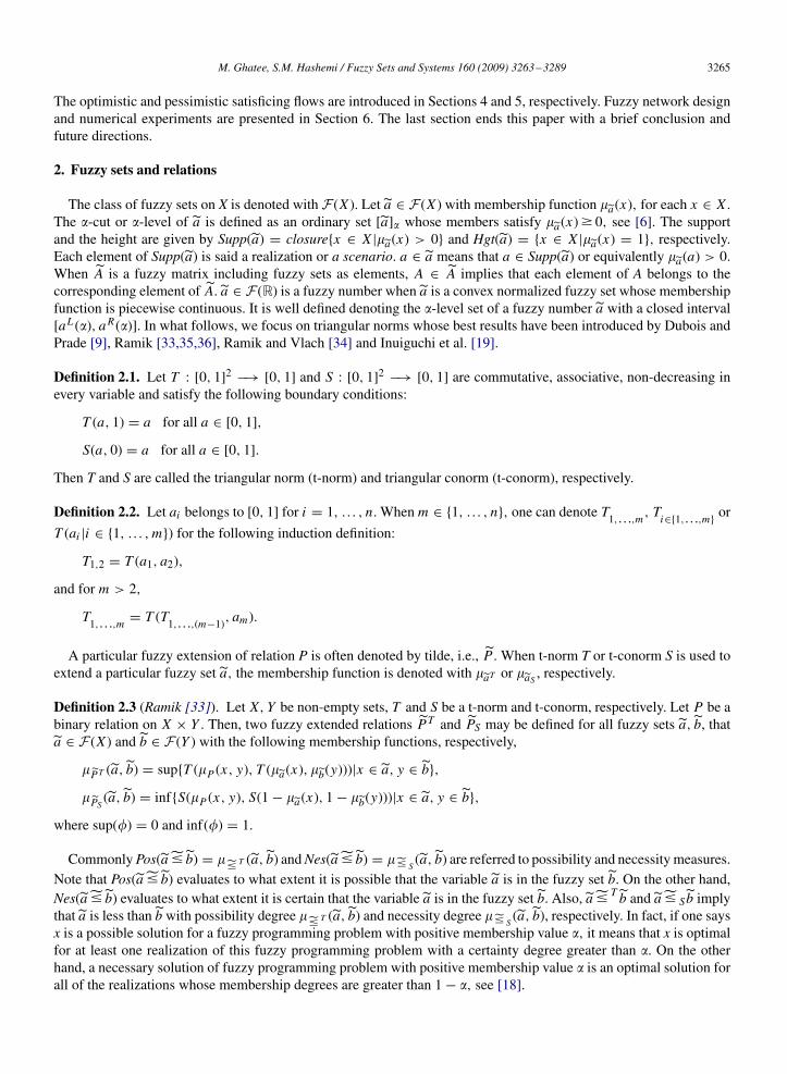
Fig. 9. (a) The convergence trend through genetic algorithm when MOMS is used in lower level of the proposed scheme of network design. (b)shows same results when MPMS algorithm is used in lower level.

Fig. 10. The values of objective functions and their goals, (a) is referred to the first objective function and (b) is referred to the second one.

respect to industrial experts, but it can be similarly done for each level of certainty degree. When MOMS algorithm isused, the proposed genetic algorithm consumes 1716.188000s in which 12690 times MOMS is loaded. The trend ofconvergence of genetic algorithm under optimistic attitude is depicted in Fig. 9a.In the case of using MPMS algorithm in network design algorithm for great Khorasan state network, according to

Figs. 10 and 11, the first objective function satisfies its goal before satisfying the second objective function by thecorresponding goal. It shows that by a higher possibility we can satisfy the first goal in comparison with the secondgoal. The networks corresponding to the optimistic and pessimistic attitudes are also depicted in Fig. 11a and b. Thedotted links of Fig. 11 are those links which should be inserted to the current network to satisfy the supply–demandconstraints whenMOMS algorithm andMPMS algorithm are used. Note that since the data are random not real values,we cannot present a judgment about the reasonability of solution, however, this implementation shows that it is possibleto find solutions for large-scale network design under fuzziness by applying the algorithms MOMS and MPMS.As a final point, it is worthwhile to note that, in some cases, when the network has been constructed and the manager

needs to extend this network, a sensitivity analysis scheme can be utilized on the proposed algorithms of this paperto provide appropriate solution(s) which are referred to next works. Also when there is conflicting between objectivefunctions, it is more reasonable to take a weighted sum of objective functions and goal values into account.


Fig. 11. Dotted links are the links which should be inserted to the network to satisfy the supply–demand constraints. (a) Network design result whenMOMS algorithm is used, (b) network design result when MPMS algorithm is used.

7. Conclusion and future directions

The optimistic and pessimistic attitudes are important concepts in management. They are important for both of thesuppliers and the customers. In fact, the optimistic decision for supplier is a pessimistic result for customer and apessimistic decision for supplier causes an optimistic result for customer. In this paper, such attitudes are consideredin the solving process of a fully fuzzified multi-objective MCFP. The presented model in this paper can be applied tounderstand the fuzzy flow through a networkwhenmultiple fuzzy costs, fuzzy capacities, fuzzy supplies and fuzzy costsare captured by decision maker. Based on the fuzzy goal programming and t-norms and t-conorms, two algorithms arealso proposed to find the maximal satisficing solutions. The application of these algorithms for network design underfuzziness is also investigated. Since the network optimization is one of the new theories which has a lot of applicationsin real engineering problems especially in transportation, it is necessary to investigate fuzzy network optimization witha higher attention. Such investigation may be covered by the modeling and solution processes. In order to show thereason of this necessity, we mention two points. When the amount of supplies and demands are defined imprecisely,the flow should be fuzzy. In these cases, some reasonable defuzzifier should be employed to interpret the fuzzy flowin real network problems. Also the constraint of a lot of network optimization problems consists of a multiplication ofa crisp matrix including −1, 1 and 0 into a fuzzy flow. We need to find a promising interpretation about this matrixmultiplication coinciding with reality. On the other hand, a lot of problems of network optimization are discrete andsome of them cannot be solved in polynomial time. These problems under fuzziness which are able to capture granularinformation, cannot usually be solved with traditional fuzzy optimization algorithms. These concepts prove that weshould focus on fuzzy network optimization independent from fuzzy linear and nonlinear programming problems. Suchinvestigations reveal that which of the network optimization can be solved efficiently under fuzziness and which ofthem provides a better interpretation of real environment.In the next works, the following directions may be followed:

• Finding customized tests to find all of the efficient solutions in the last part of Algorithm MOMS and MPMS.


• Using a combination of multiple fuzzy costs when there is conflicting between objectives.• Introducingmore efficient heuristics andmeta-heuristics which can be applied to solve real large-scale fuzzy networkdesign.

Acknowledgment

The authors would like to express particular thanks to the Area Editor, Editors-in-Chief and honorable reviewers fortheir useful comments which improve the quality of paper.

References

[1] W.F. Abd El-Wahed, S.M. Lee, Interactive fuzzy goal programming for multi-objective transportation problems, Omega 34 (2006) 158–166.[2] R.K. Ahuja, T.L. Magnanti, J.B. Orlin, Network Flows, Prentice-Hall, Englewood Cliffs, 1993.[3] S.K. Bath, J.S. Dhillon, D.P. Kothari, Fuzzy satisfying stochastic multi-objective generation scheduling by weightage pattern search methods,

Electric Power Systems Research 69 (2004) 311–320.[4] P.R. Bhave, R. Gupta, Optimal design of water distribution networks for fuzzy demands, Civil Engineering and Environmental Systems 21

(2004) 229–245.[5] Y.S. Brar, J.S. Dhillon, D.P. Kothari, Fuzzy satisfying multi-objective generation scheduling based on simplex weightage pattern search,

Electrical Power and Energy Systems 27 (2005) 518–527.[6] P.T. Chang, K.C. Hung, �-Cut fuzzy arithmetic: simplifying rules and a fuzzy function optimization with a decision variable, IEEE Transactions

on Fuzzy Systems 14 (2006) 496–510.[7] S. Chanas, D. Kuchta, Fuzzy integer transportation problem, Fuzzy Sets and Systems 98 (1998) 291–298.[8] M. Chen, H. Ishii, C.Wu, Transportation problems on a fuzzy network, International Journal of Innovative Computing, Information and Control

4 (2008) 1105–1109.[9] D. Dubois, H. Prade, Fuzzy Sets and Systems: Theory and Applications, Academic Press, New York, 1980.[10] D. Dubois, H. Prade, Possibility Theory, Plenum Press, New York, 1988.[11] M. Gen, R. Cheng, Genetic Algorithms and Engineering Optimization, Wiley, New York, 2000.[12] M. Ghatee, S.M. Hashemi, Ranking function-based solutions of fully fuzzified minimal cost flow problem, Information Sciences 177 (2007)

4271–4294.[13] M. Ghatee, S.M. Hashemi, Generalized minimal cost flow problem in fuzzy nature: an application in bus network planning problem, Applied

Mathematical Modelling 32 (2008) 2490–2508.[14] M. Ghatee, S.M. Hashemi, B. Hashemi, M. Dehghan, Solution and duality of imprecise network problems, Computers and Mathematics with

Applications 55 (2008) 2767–2790.[15] H.W.Hamacher, C.R. Pedersen, S. Ruzika,Multiple objectiveminimum cost flow problems: a review, European Journal of Operational Research

176 (2007) 1404–1422.[16] S.M. Hashemi, M. Ghatee, B. Hashemi, Fuzzy goal programming: complementary slackness conditions and computational schemes, Applied

Mathematics and Computation 179 (2006) 506–522.[17] F. Hernandes, M.T. Lamata, J.L. Verdegay, A. Yamakami, The shortest path problem on networks with fuzzy parameters, Fuzzy Sets and

Systems 158 (2007) 1561–1570.[18] M. Inuiguchi, M. Sakawa, Possible and necessary optimality tests in possibilistic linear programming problems, Fuzzy Sets and Systems 67

(1994) 29–46.[19] M. Inuiguchi, J. Ramik, T. Tanino,M. Vlach, Satisficing solutions and duality in interval and fuzzy linear programming, Fuzzy Sets and Systems

135 (2003) 151–177.[20] M. Inuiguchi, Necessity measure optimization in linear programming problems with fuzzy polytopes, Fuzzy Sets and Systems 158 (2007)

1882–1891.[21] F. Jimenez, J.L. Verdegay, Solving fuzzy solid transportation problems by an evolutionary algorithm based parametric approach, European

Journal of Operational Research 117 (1999) 485–510.[22] B. Julien, An extension to possibilistic linear programming, Fuzzy Sets and Systems 64 (1994) 195–206.[23] D.P. Kothari, J.S. Dhillon, Power System Optimization, Prentice-Hall, India, 2004.[24] S. Li, C. Hu, Two-step interactive satisfactory method for fuzzy multiple objective optimization with preemptive priorities, IEEE Transactions

on Fuzzy Systems 15 (2007) 417–425.[25] Y. Li, K. Ida, M. Gen, Improved genetic algorithm for solving multiobjective solid transportation problem with fuzzy numbers, Computers &

Industrial Engineering 33 (1997) 589–592.[26] T.F. Liang, Interactive multi-objective transportation planning decisions using fuzzy linear programming, Asia-Pacific Journal of Operational

Research 25 (2008) 11–31.[27] S.T. Liu, C. Kao, Solving fuzzy transportation problems based on extension principle, European Journal of Operational Research 153 (2003)

661–674.[28] S.T. Liu, C. Kao, Network flow problems with fuzzy arc lengths, IEEE Transactions on Systems, Man and Cybernetics–Part B: Cybernetics 34

(2004) 765–769.[29] X. Liu, Measuring the satisfaction of constraints in fuzzy linear programming, Fuzzy Sets and Systems 122 (2001) 263–275.


[30] J.A.M. Perez, J.M.M. Vega, J.L. Verdegay, Fuzzy location problems on networks, Fuzzy Sets and Systems 142 (2004) 393–405.[31] J. Ramik, H. Rommelfanger, Fuzzy mathematical programming based on some new inequality relations, Fuzzy Sets and Systems 81 (1996)

77–88.[32] J. Ramik, Multi-index transportation problem with fuzzy coefficients and fuzzy decision variables, Tatra Mountains Mathematical Publications

12 (1997) 151–168.[33] J. Ramik, Fuzzy goals and fuzzy alternatives in goal programming problems, Fuzzy Sets and Systems 111 (2000) 81–86.[34] J. Ramik, M. Vlach, Generalized Concavity in Fuzzy Optimization and Decision Analysis, Kluwer Academic Publishers, Dordrecht, Boston,

London, 2002.[35] J. Ramik, Duality in fuzzy linear programming with possibility and necessity relations, Fuzzy Sets and Systems 157 (2006) 1283–1302.[36] J. Ramik, Optimal solutions in optimization problem with objective function depending on fuzzy parameters, Fuzzy Sets and Systems 158

(2007) 1873–1881.[37] N. Safaei,M. Saidi-Mehrabad, R. Tavakkoli-Moghaddam, F. Sassani, A fuzzy programming approach for a cell formation problemwith dynamic

and uncertain conditions, Fuzzy Sets and Systems 159 (2008) 215–236.[38] H.S. Shih, E.S. Lee, Fuzzy multi-level minimum cost flow problems, Fuzzy Sets and Systems 107 (1999) 159–176.[39] L.H. Shih, Cement transportation planning via fuzzy linear programming, International Journal of Production Economics 58 (1999) 277–287.[40] B.L. Smith, W.T. Scherer, J.H. Conklin, Exploring imputation techniques for missing data in transportation management systems, in: 82nd

Annu. Meeting of the Transportation Research Board, 2002.[41] H. Tanaka, P. Guo, H.J. Zimmermann, Possibility distributions of fuzzy decision variables obtained from possibilistic linear programming

problems, Fuzzy Sets and Systems 113 (2000) 323–332.[42] S.A. Torabi, E. Hassini, An interactive possibilistic programming approach for multiple objective supply chain master planning, Fuzzy Sets

and Systems 159 (2008) 193–214.[43] G.-H. Tzeng, D. Teodorovi, M.-J. Hwang, Fuzzy bicriteria multi-index transportation problems for coal allocation planning of Taipower,

European Journal of Operational Research 95 (1996) 62–72.[44] L.A. Zadeh, Fuzzy sets as a basis for a theory of possibility, Fuzzy Sets and Systems 1 (1978) 3–28.[45] M. Zeleny, Multiple Criteria Decision Making, McGraw-Hill, New York, 1982.

Documents

Application of fuzzy minimum cost flow problems to network design under uncertainty