Graduate Theses, Dissertations, and Problem Reports

2020

Application of Flowing Material Balance in Unconventional Application of Flowing Material Balance in Unconventional

Reservoirs Reservoirs

Salem Alharbi saalharbi@mix.wvu.edu

Follow this and additional works at: https://researchrepository.wvu.edu/etd

Part of the Petroleum Engineering Commons

Recommended Citation Recommended Citation Alharbi, Salem, "Application of Flowing Material Balance in Unconventional Reservoirs" (2020). Graduate Theses, Dissertations, and Problem Reports. 7881. https://researchrepository.wvu.edu/etd/7881

This Problem/Project Report is protected by copyright and/or related rights. It has been brought to you by the The Research Repository @ WVU with permission from the rights-holder(s). You are free to use this Problem/Project Report in any way that is permitted by the copyright and related rights legislation that applies to your use. For other uses you must obtain permission from the rights-holder(s) directly, unless additional rights are indicated by a Creative Commons license in the record and/ or on the work itself. This Problem/Project Report has been accepted for inclusion in WVU Graduate Theses, Dissertations, and Problem Reports collection by an authorized administrator of The Research Repository @ WVU. For more information, please contact researchrepository@mail.wvu.edu.

Application of Flowing Material Balance in Unconventional Reservoirs

Salem Alharbi

Problem Report submitted to the

Benjamin M. Statler College of Engineering and Mineral Resources at West Virginia University

In partial fulfillment for the degree of Master of Science in Petroleum and Natural Gas Engineering

Kashy Aminian, PhD, Chair Samuel Ameri, PhD

Ming Gu, PhD

Department of Petroleum and Natural Gas Engineering, Morgantown, West Virginia

2020

Keywords: Flowing Material Balance, Gas in Place, Unconventional Reservoir

Copyright: 2020 Salem Alharbi

Abstract Application of Flowing Material Balance in Unconventional

Reservoirs

Salem Alharbi

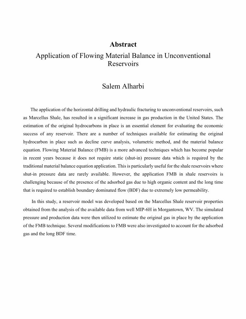
The application of the horizontal drilling and hydraulic fracturing to unconventional reservoirs, such

as Marcellus Shale, has resulted in a significant increase in gas production in the United States. The

estimation of the original hydrocarbons in place is an essential element for evaluating the economic

success of any reservoir. There are a number of techniques available for estimating the original

hydrocarbon in place such as decline curve analysis, volumetric method, and the material balance

equation. Flowing Material Balance (FMB) is a more advanced techniques which has become popular

in recent years because it does not require static (shut-in) pressure data which is required by the

traditional material balance equation application. This is particularly useful for the shale reservoirs where

shut-in pressure data are rarely available. However, the application FMB in shale reservoirs is

challenging because of the presence of the adsorbed gas due to high organic content and the long time

that is required to establish boundary dominated flow (BDF) due to extremely low permeability.

In this study, a reservoir model was developed based on the Marcellus Shale reservoir properties

obtained from the analysis of the available data from well MIP-6H in Morgantown, WV. The simulated

pressure and production data were then utilized to estimate the original gas in place by the application

of the FMB technique. Several modifications to FMB were also investigated to account for the adsorbed

gas and the long BDF time.

iii

Acknowledgement

I want to express my gratitude and appreciation to my research advisor Dr. Kashy Aminian for his

support and motivation during my graduate program. With his help and guidance, I was able to complete

my research.

Also, I would like to thank professor. Sam, for his support and motivation through my graduate program.

Finally, I want to thank my family and friends for their prayer and support, which led me to achieve my

goal and complete my master's degree.

iv

Contents Abstract ......................................................................................................................................................................... ii

Acknowledgement ........................................................................................................................................................ iii

Table of Figures ............................................................................................................................................................ v

List of Tables ................................................................................................................................................................ vi

Nomenclature .............................................................................................................................................................. vii

Chapter 1: Introduction ................................................................................................................................................. 1

Chapter 2: Literature Review ........................................................................................................................................ 2

2.1: Material Balance Equation (MBE) ......................................................................................................................... 2

2.2: Flowing Material Balance for Gas Reservoir ......................................................................................................... 2

2.3: King Method .......................................................................................................................................................... 3

2.4: Clarkson and McGovern Method ........................................................................................................................... 4

2.5: Horizontal Well with Multi-Stage Fractures .......................................................................................................... 5

2.6: CMG Model ........................................................................................................................................................... 6

Chapter 3: Methodology ................................................................................................................................................ 8

3.1. Simulated Pressure and Production Data for a Marcellus Shale Horizontal Well .................................................. 8

3.2. Gas in Place Estimation by the Conventional FMB ............................................................................................. 10

3.3. Gas in Place Estimation by the King Method ....................................................................................................... 10

3.4. Gas in Place Estimation by the Clarkson-McGovern Method .............................................................................. 11

Chapter 4: Results and Discussion .............................................................................................................................. 12

4.1: Model 1 Results .................................................................................................................................................... 12

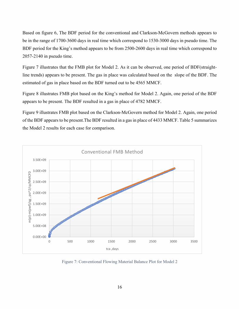
4.2: Model 2 Results .................................................................................................................................................... 15

Chapter 5: Conclusion and Recommendations ............................................................................................................ 19

References ................................................................................................................................................................... 20

v

Table of Figures

Figure 1: Flow Regimes for Horizontal Well with Multi-Stage Fractures ............................................... 6

Figure 2: Well bottomhole Pressure Profile for Model 1 ....................................................................... 12

Figure 3 : Conventional Flowing Material Balance Plot for Model 1 .................................................... 13

Figure 4: King Flowing Material Balance Plot for Model 1 .................................................................. 14

Figure 5: Clarkson-McGovern Flowing Material Balance Plot for Model 1 ......................................... 14

Figure 6: Well bottomhole Pressure Profile for Model 2 ....................................................................... 15

Figure 7: Conventional Flowing Material Balance Plot for Model 2 ..................................................... 16

Figure 8: King Flowing Material Balance Plot for Model 2 .................................................................. 17

Figure 9: Clarkson-McGovern Flowing Material Balance Plot for Model 2 ......................................... 17

vi

List of Tables

Table 1: Model 1 Reservoir Properties ..................................................................................................... 9

Table 2: Model 1 Hydraulic Fractures Properties ..................................................................................... 9

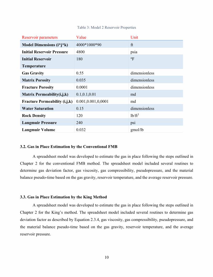
Table 3: Model 2 Reservoir Properties ................................................................................................... 10

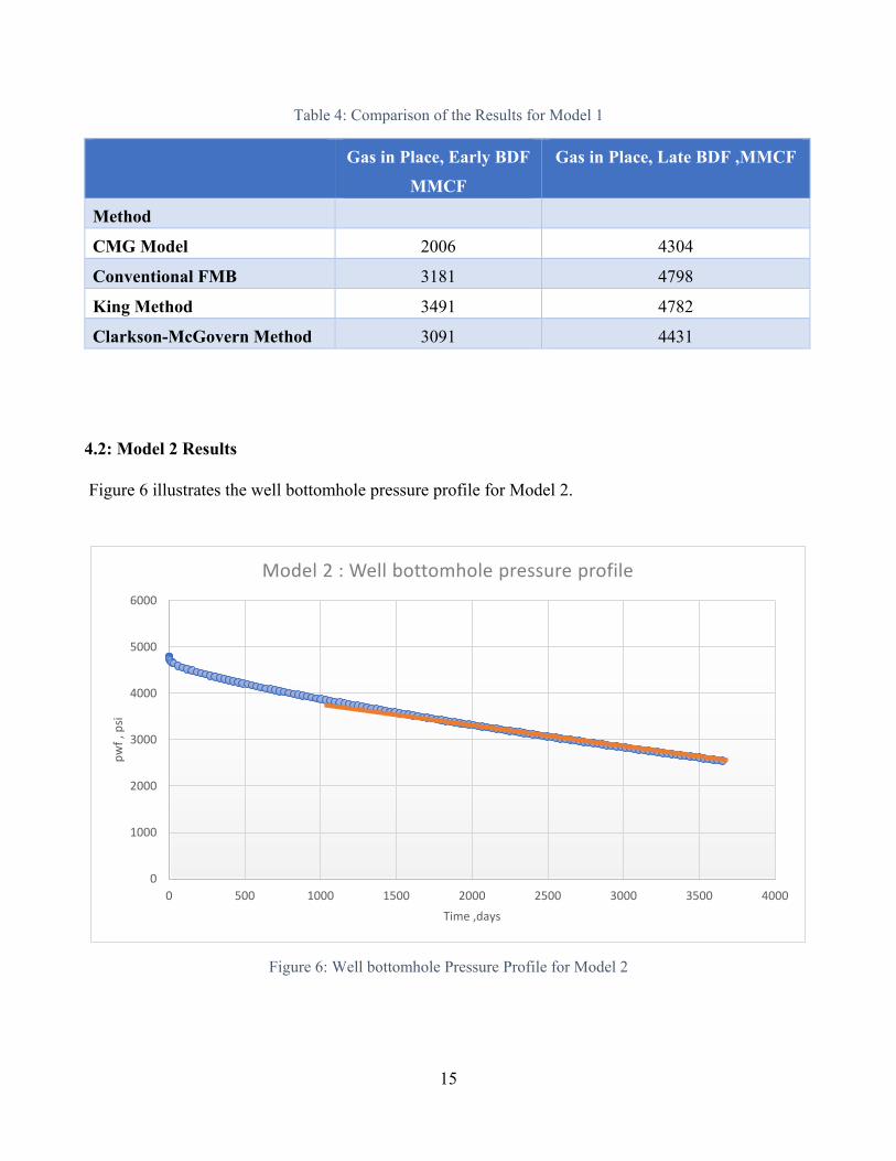
Table 4: Comparison of the Results for Model 1 ................................................................................... 15

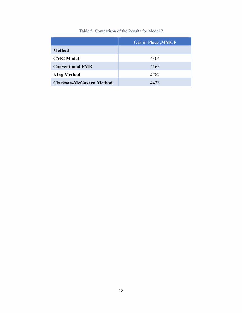
Table 5: Comparison of the Results for Model 2 ................................................................................... 18

vii

Nomenclature

𝐵𝐵𝑔𝑔 = 𝑔𝑔𝑔𝑔𝑔𝑔 𝑓𝑓𝑓𝑓𝑓𝑓𝑓𝑓𝑔𝑔𝑓𝑓𝑓𝑓𝑓𝑓𝑓𝑓 𝑣𝑣𝑓𝑓𝑣𝑣𝑣𝑣𝑓𝑓𝑣𝑣 𝑓𝑓𝑔𝑔𝑓𝑓𝑓𝑓𝑓𝑓𝑓𝑓 , 𝑓𝑓𝑓𝑓𝑓𝑓/𝑔𝑔𝑓𝑓𝑓𝑓

𝐵𝐵𝑔𝑔𝑔𝑔 = 𝑔𝑔𝑔𝑔𝑔𝑔 𝑓𝑓𝑓𝑓𝑓𝑓𝑓𝑓𝑔𝑔𝑓𝑓𝑓𝑓𝑓𝑓𝑓𝑓 𝑣𝑣𝑓𝑓𝑣𝑣𝑣𝑣𝑓𝑓𝑣𝑣 𝑓𝑓𝑔𝑔𝑓𝑓𝑓𝑓𝑓𝑓𝑓𝑓 𝑔𝑔𝑓𝑓 𝑓𝑓𝑓𝑓𝑓𝑓𝑓𝑓𝑓𝑓𝑔𝑔𝑣𝑣 𝑝𝑝𝑓𝑓𝑣𝑣𝑔𝑔𝑔𝑔𝑣𝑣𝑓𝑓𝑣𝑣 , 𝑓𝑓𝑓𝑓𝑓𝑓/𝑔𝑔𝑓𝑓𝑓𝑓

𝐵𝐵𝑤𝑤 = 𝑤𝑤𝑔𝑔𝑓𝑓𝑣𝑣𝑓𝑓 𝑓𝑓𝑓𝑓𝑓𝑓𝑓𝑓𝑔𝑔𝑓𝑓𝑓𝑓𝑓𝑓𝑓𝑓 𝑣𝑣𝑓𝑓𝑣𝑣𝑣𝑣𝑓𝑓𝑣𝑣 𝑓𝑓𝑔𝑔𝑓𝑓𝑓𝑓𝑓𝑓𝑓𝑓 , 𝑓𝑓𝑓𝑓𝑓𝑓/𝑔𝑔𝑓𝑓𝑓𝑓

𝑏𝑏𝑝𝑝𝑝𝑝𝑝𝑝 = 𝑅𝑅𝑣𝑣𝑔𝑔𝑣𝑣𝑓𝑓𝑣𝑣𝑓𝑓𝑓𝑓𝑓𝑓 𝑓𝑓𝑓𝑓𝑓𝑓𝑔𝑔𝑓𝑓𝑔𝑔𝑓𝑓𝑓𝑓 (𝑝𝑝𝑔𝑔𝑣𝑣𝑣𝑣𝑝𝑝𝑓𝑓 𝑔𝑔𝑓𝑓𝑣𝑣𝑔𝑔𝑝𝑝𝑠𝑠 𝑔𝑔𝑓𝑓𝑔𝑔𝑓𝑓𝑣𝑣)

𝑓𝑓𝑓𝑓 = 𝑓𝑓𝑓𝑓𝑓𝑓𝑓𝑓𝑔𝑔𝑓𝑓𝑓𝑓𝑓𝑓𝑓𝑓 𝑓𝑓𝑓𝑓𝑓𝑓𝑝𝑝𝑓𝑓𝑣𝑣𝑔𝑔𝑔𝑔𝑓𝑓𝑏𝑏𝑣𝑣𝑓𝑓𝑓𝑓𝑠𝑠 ,1/𝑝𝑝𝑔𝑔𝑓𝑓

𝑓𝑓𝑔𝑔 = 𝑔𝑔𝑔𝑔𝑔𝑔 𝑓𝑓𝑓𝑓𝑓𝑓𝑝𝑝𝑓𝑓𝑣𝑣𝑔𝑔𝑔𝑔𝑓𝑓𝑏𝑏𝑣𝑣𝑓𝑓𝑓𝑓𝑠𝑠 ,1/𝑝𝑝𝑔𝑔𝑓𝑓

𝑓𝑓𝑔𝑔𝑔𝑔 = 𝑔𝑔𝑔𝑔𝑔𝑔 𝑓𝑓𝑓𝑓𝑓𝑓𝑝𝑝𝑓𝑓𝑣𝑣𝑔𝑔𝑔𝑔𝑓𝑓𝑏𝑏𝑣𝑣𝑓𝑓𝑓𝑓𝑠𝑠 𝑔𝑔𝑓𝑓 𝑓𝑓𝑓𝑓𝑓𝑓𝑓𝑓𝑓𝑓𝑔𝑔𝑣𝑣 𝑝𝑝𝑓𝑓𝑣𝑣𝑔𝑔𝑔𝑔𝑣𝑣𝑓𝑓𝑣𝑣 ,1/𝑝𝑝𝑔𝑔𝑓𝑓

𝑓𝑓𝑡𝑡 = 𝑓𝑓𝑓𝑓𝑓𝑓𝑔𝑔𝑣𝑣 𝑓𝑓𝑓𝑓𝑓𝑓𝑝𝑝𝑓𝑓𝑣𝑣𝑔𝑔𝑔𝑔𝑓𝑓𝑏𝑏𝑣𝑣𝑓𝑓𝑓𝑓𝑠𝑠 ,1/𝑝𝑝𝑔𝑔𝑓𝑓

𝑓𝑓𝑡𝑡𝑔𝑔 = 𝑓𝑓𝑓𝑓𝑓𝑓𝑔𝑔𝑣𝑣 𝑓𝑓𝑓𝑓𝑓𝑓𝑝𝑝𝑓𝑓𝑣𝑣𝑔𝑔𝑔𝑔𝑓𝑓𝑏𝑏𝑣𝑣𝑓𝑓𝑓𝑓𝑠𝑠 𝑔𝑔𝑓𝑓 𝑓𝑓𝑓𝑓𝑓𝑓𝑓𝑓𝑓𝑓𝑔𝑔𝑣𝑣 𝑝𝑝𝑓𝑓𝑣𝑣𝑔𝑔𝑔𝑔𝑣𝑣𝑓𝑓𝑣𝑣 ,1/𝑝𝑝𝑔𝑔𝑓𝑓

𝑓𝑓𝑤𝑤 = 𝑤𝑤𝑔𝑔𝑓𝑓𝑣𝑣𝑓𝑓 𝑓𝑓𝑓𝑓𝑓𝑓𝑝𝑝𝑓𝑓𝑣𝑣𝑔𝑔𝑔𝑔𝑓𝑓𝑏𝑏𝑣𝑣𝑓𝑓𝑓𝑓𝑠𝑠 ,1/𝑝𝑝𝑔𝑔𝑓𝑓

𝐺𝐺 = 𝑓𝑓𝑓𝑓𝑓𝑓𝑓𝑓𝑓𝑓𝑔𝑔𝑣𝑣 𝑔𝑔𝑔𝑔𝑔𝑔 𝑓𝑓𝑓𝑓 𝑝𝑝𝑣𝑣𝑔𝑔𝑓𝑓𝑣𝑣 ,𝑀𝑀𝑀𝑀𝑀𝑀𝑀𝑀

𝐺𝐺𝑝𝑝 = 𝑓𝑓𝑣𝑣𝑓𝑓𝑣𝑣𝑣𝑣𝑔𝑔𝑓𝑓𝑓𝑓𝑣𝑣𝑣𝑣 𝑔𝑔𝑔𝑔𝑔𝑔 𝑝𝑝𝑓𝑓𝑓𝑓𝑝𝑝𝑣𝑣𝑓𝑓𝑓𝑓𝑓𝑓𝑓𝑓𝑓𝑓,𝑀𝑀𝑀𝑀𝑀𝑀𝑀𝑀

h = formation thickness, ft

k= permeability, md

𝑓𝑓(𝑝𝑝𝑔𝑔) = 𝑝𝑝𝑔𝑔𝑣𝑣𝑣𝑣𝑝𝑝𝑓𝑓 𝑝𝑝𝑓𝑓𝑣𝑣𝑔𝑔𝑔𝑔𝑣𝑣𝑓𝑓𝑣𝑣 𝑔𝑔𝑓𝑓 𝑓𝑓𝑓𝑓𝑓𝑓𝑓𝑓𝑓𝑓𝑔𝑔𝑣𝑣 𝑝𝑝𝑓𝑓𝑣𝑣𝑔𝑔𝑔𝑔𝑣𝑣𝑓𝑓𝑣𝑣 ,𝑝𝑝𝑔𝑔𝑓𝑓2/𝑓𝑓𝑝𝑝

𝑓𝑓�𝑝𝑝𝑤𝑤𝑓𝑓� = 𝑤𝑤𝑣𝑣𝑣𝑣𝑣𝑣 𝑏𝑏𝑓𝑓𝑓𝑓𝑓𝑓𝑓𝑓𝑓𝑓𝑓𝑓ℎ𝑓𝑓𝑣𝑣𝑣𝑣 𝑓𝑓𝑣𝑣𝑓𝑓𝑤𝑤𝑓𝑓𝑓𝑓𝑔𝑔 𝑝𝑝𝑔𝑔𝑣𝑣𝑣𝑣𝑝𝑝𝑓𝑓 𝑝𝑝𝑓𝑓𝑣𝑣𝑔𝑔𝑔𝑔𝑣𝑣𝑓𝑓𝑣𝑣 ,𝑝𝑝𝑔𝑔𝑓𝑓2/𝑓𝑓𝑝𝑝

𝑓𝑓(𝑝𝑝𝑝) = 𝑔𝑔𝑣𝑣𝑣𝑣𝑓𝑓𝑔𝑔𝑔𝑔𝑣𝑣 𝑓𝑓𝑣𝑣𝑔𝑔𝑣𝑣𝑓𝑓𝑣𝑣𝑓𝑓𝑓𝑓𝑓𝑓 𝑝𝑝𝑔𝑔𝑣𝑣𝑣𝑣𝑝𝑝𝑓𝑓 𝑝𝑝𝑓𝑓𝑣𝑣𝑔𝑔𝑔𝑔𝑣𝑣𝑓𝑓𝑣𝑣 , 𝑝𝑝𝑔𝑔𝑓𝑓2/𝑓𝑓𝑝𝑝

𝑓𝑓(𝑝𝑝) = 𝑝𝑝𝑔𝑔𝑣𝑣𝑣𝑣𝑝𝑝𝑓𝑓 𝑝𝑝𝑓𝑓𝑣𝑣𝑔𝑔𝑔𝑔𝑣𝑣𝑓𝑓𝑣𝑣 ,𝑝𝑝𝑔𝑔𝑓𝑓2/𝑓𝑓𝑝𝑝

p𝑝= average pressure, psia

p= pressure, psia

𝑝𝑝𝐿𝐿 = 𝐿𝐿𝑔𝑔𝑓𝑓𝑔𝑔𝑓𝑓𝑣𝑣𝑓𝑓𝑓𝑓 𝑝𝑝𝑓𝑓𝑣𝑣𝑔𝑔𝑔𝑔𝑣𝑣𝑓𝑓𝑣𝑣 ,𝑝𝑝𝑔𝑔𝑓𝑓𝑔𝑔

𝑝𝑝𝑔𝑔 = 𝑓𝑓𝑓𝑓𝑓𝑓𝑓𝑓𝑓𝑓𝑔𝑔𝑣𝑣 𝑓𝑓𝑣𝑣𝑔𝑔𝑣𝑣𝑓𝑓𝑣𝑣𝑓𝑓𝑓𝑓𝑓𝑓 𝑝𝑝𝑓𝑓𝑣𝑣𝑔𝑔𝑔𝑔𝑣𝑣𝑓𝑓𝑣𝑣,𝑝𝑝𝑔𝑔𝑓𝑓𝑔𝑔

𝑝𝑝𝑤𝑤𝑓𝑓 = 𝑤𝑤𝑣𝑣𝑣𝑣𝑣𝑣 𝑏𝑏𝑓𝑓𝑓𝑓𝑓𝑓𝑓𝑓𝑓𝑓ℎ𝑓𝑓𝑣𝑣𝑣𝑣 𝑝𝑝𝑓𝑓𝑣𝑣𝑔𝑔𝑔𝑔𝑣𝑣𝑓𝑓𝑣𝑣, 𝑝𝑝𝑔𝑔𝑓𝑓𝑔𝑔

𝑞𝑞𝑔𝑔 = 𝑔𝑔𝑔𝑔𝑔𝑔 𝑓𝑓𝑣𝑣𝑓𝑓𝑤𝑤 𝑓𝑓𝑔𝑔𝑓𝑓𝑣𝑣 ,𝑀𝑀𝑀𝑀𝑀𝑀𝑀𝑀𝑀𝑀

𝑓𝑓𝑒𝑒 = 𝑝𝑝𝑓𝑓𝑔𝑔𝑓𝑓𝑓𝑓𝑔𝑔𝑔𝑔𝑣𝑣 𝑓𝑓𝑔𝑔𝑝𝑝𝑓𝑓𝑣𝑣𝑔𝑔 ,𝑓𝑓𝑓𝑓

𝑓𝑓𝑤𝑤 = 𝑤𝑤𝑣𝑣𝑣𝑣𝑣𝑣𝑏𝑏𝑓𝑓𝑓𝑓𝑣𝑣 𝑓𝑓𝑔𝑔𝑝𝑝𝑓𝑓𝑣𝑣𝑔𝑔 ,𝑓𝑓𝑓𝑓

𝑓𝑓𝑤𝑤𝑤𝑤 = 𝑔𝑔𝑝𝑝𝑝𝑝𝑔𝑔𝑓𝑓𝑣𝑣𝑓𝑓𝑓𝑓 𝑤𝑤𝑣𝑣𝑣𝑣𝑣𝑣𝑏𝑏𝑓𝑓𝑓𝑓𝑣𝑣 𝑓𝑓𝑔𝑔𝑝𝑝𝑓𝑓𝑣𝑣𝑔𝑔 ,𝑓𝑓𝑓𝑓 , 𝑓𝑓𝑤𝑤𝑤𝑤 = 𝑓𝑓𝑤𝑤𝑣𝑣−𝑝𝑝

viii

𝑆𝑆𝑤𝑤 = 𝑤𝑤𝑔𝑔𝑓𝑓𝑣𝑣𝑓𝑓 𝑔𝑔𝑔𝑔𝑓𝑓𝑣𝑣𝑓𝑓𝑔𝑔𝑓𝑓𝑓𝑓𝑓𝑓𝑓𝑓 ,𝑝𝑝𝑓𝑓𝑓𝑓𝑣𝑣𝑓𝑓𝑔𝑔𝑓𝑓𝑓𝑓𝑓𝑓𝑣𝑣𝑣𝑣𝑔𝑔𝑔𝑔

𝑆𝑆𝑤𝑤𝑔𝑔 = 𝑓𝑓𝑓𝑓𝑓𝑓𝑣𝑣𝑝𝑝𝑣𝑣𝑓𝑓𝑓𝑓𝑏𝑏𝑣𝑣𝑣𝑣 𝑤𝑤𝑔𝑔𝑓𝑓𝑣𝑣𝑓𝑓 𝑔𝑔𝑔𝑔𝑓𝑓𝑣𝑣𝑓𝑓𝑔𝑔𝑓𝑓𝑓𝑓𝑓𝑓𝑓𝑓 ,𝑝𝑝𝑓𝑓𝑓𝑓𝑣𝑣𝑓𝑓𝑔𝑔𝑓𝑓𝑓𝑓𝑓𝑓𝑣𝑣𝑣𝑣𝑔𝑔𝑔𝑔

T= Temperature,°R

𝑓𝑓𝑐𝑐𝑤𝑤 = 𝑔𝑔𝑝𝑝𝑎𝑎𝑣𝑣𝑔𝑔𝑓𝑓𝑣𝑣𝑝𝑝 𝑓𝑓𝑔𝑔𝑓𝑓𝑣𝑣𝑓𝑓𝑓𝑓𝑔𝑔𝑣𝑣 𝑏𝑏𝑔𝑔𝑣𝑣𝑔𝑔𝑓𝑓𝑓𝑓𝑣𝑣 𝑝𝑝𝑔𝑔𝑣𝑣𝑣𝑣𝑝𝑝𝑓𝑓 𝑓𝑓𝑓𝑓𝑓𝑓𝑣𝑣 , days

𝑣𝑣𝑔𝑔 = 𝑔𝑔𝑔𝑔𝑔𝑔 𝑣𝑣𝑓𝑓𝑔𝑔𝑓𝑓𝑓𝑓𝑔𝑔𝑓𝑓𝑓𝑓𝑠𝑠 , 𝑓𝑓𝑝𝑝

𝑣𝑣𝑔𝑔𝑔𝑔 = 𝑔𝑔𝑔𝑔𝑔𝑔 𝑣𝑣𝑓𝑓𝑔𝑔𝑓𝑓𝑓𝑓𝑔𝑔𝑓𝑓𝑓𝑓𝑠𝑠 𝑔𝑔𝑓𝑓 𝑓𝑓𝑓𝑓𝑓𝑓𝑓𝑓𝑓𝑓𝑔𝑔𝑣𝑣 𝑝𝑝𝑓𝑓𝑣𝑣𝑔𝑔𝑔𝑔𝑣𝑣𝑓𝑓𝑣𝑣 , 𝑓𝑓𝑝𝑝

𝑉𝑉𝐿𝐿 = 𝐿𝐿𝑔𝑔𝑓𝑓𝑔𝑔𝑓𝑓𝑣𝑣𝑓𝑓𝑓𝑓 𝑣𝑣𝑓𝑓𝑣𝑣𝑣𝑣𝑓𝑓𝑣𝑣 , 𝑔𝑔𝑓𝑓𝑓𝑓/𝑓𝑓𝑓𝑓𝑓𝑓

𝑊𝑊𝑒𝑒 = 𝑤𝑤𝑔𝑔𝑓𝑓𝑣𝑣𝑓𝑓 𝑓𝑓𝑓𝑓𝑓𝑓𝑣𝑣𝑣𝑣𝑖𝑖 , 𝑓𝑓𝑏𝑏

𝑊𝑊𝑝𝑝 = 𝑤𝑤𝑔𝑔𝑓𝑓𝑣𝑣𝑓𝑓 𝑝𝑝𝑓𝑓𝑓𝑓𝑝𝑝𝑣𝑣𝑓𝑓𝑓𝑓𝑓𝑓𝑓𝑓𝑓𝑓, 𝑆𝑆𝑆𝑆𝐵𝐵

𝑧𝑧 = 𝑝𝑝𝑣𝑣𝑣𝑣𝑓𝑓𝑔𝑔𝑓𝑓𝑓𝑓𝑓𝑓𝑓𝑓 𝑓𝑓𝑔𝑔𝑓𝑓𝑓𝑓𝑓𝑓𝑓𝑓 ,𝑝𝑝𝑓𝑓𝑓𝑓𝑣𝑣𝑓𝑓𝑔𝑔𝑓𝑓𝑓𝑓𝑓𝑓𝑣𝑣𝑣𝑣𝑔𝑔𝑔𝑔

𝑧𝑧∗ = 𝑝𝑝𝑣𝑣𝑣𝑣𝑓𝑓𝑔𝑔𝑓𝑓𝑓𝑓𝑓𝑓𝑓𝑓 𝑓𝑓𝑔𝑔𝑓𝑓𝑓𝑓𝑓𝑓𝑓𝑓 𝑓𝑓𝑓𝑓𝑓𝑓 𝑣𝑣𝑓𝑓𝑓𝑓𝑓𝑓𝑓𝑓𝑣𝑣𝑣𝑣𝑓𝑓𝑓𝑓𝑓𝑓𝑓𝑓𝑓𝑓𝑔𝑔𝑣𝑣 𝑓𝑓𝑣𝑣𝑔𝑔𝑣𝑣𝑓𝑓𝑣𝑣𝑓𝑓𝑓𝑓𝑓𝑓 ,𝑝𝑝𝑓𝑓𝑓𝑓𝑣𝑣𝑓𝑓𝑔𝑔𝑓𝑓𝑓𝑓𝑓𝑓𝑣𝑣𝑣𝑣𝑔𝑔𝑔𝑔

𝑧𝑧𝑔𝑔 = 𝑝𝑝𝑣𝑣𝑣𝑣𝑓𝑓𝑔𝑔𝑓𝑓𝑓𝑓𝑓𝑓𝑓𝑓 𝑓𝑓𝑔𝑔𝑓𝑓𝑓𝑓𝑓𝑓𝑓𝑓 𝑔𝑔𝑓𝑓 𝑓𝑓𝑓𝑓𝑓𝑓𝑓𝑓𝑓𝑓𝑔𝑔𝑣𝑣 𝑝𝑝𝑓𝑓𝑣𝑣𝑔𝑔𝑔𝑔𝑣𝑣𝑓𝑓𝑣𝑣 ,𝑝𝑝𝑓𝑓𝑓𝑓𝑣𝑣𝑓𝑓𝑔𝑔𝑓𝑓𝑓𝑓𝑓𝑓𝑣𝑣𝑣𝑣𝑔𝑔𝑔𝑔

𝜌𝜌𝑏𝑏 = 𝑏𝑏𝑣𝑣𝑣𝑣𝑏𝑏 𝑝𝑝𝑣𝑣𝑓𝑓𝑔𝑔𝑓𝑓𝑓𝑓𝑠𝑠 , 𝑔𝑔𝑓𝑓𝑓𝑓/𝑓𝑓𝑓𝑓𝑓𝑓

∅ = 𝑝𝑝𝑓𝑓𝑓𝑓𝑓𝑓𝑔𝑔𝑓𝑓𝑓𝑓𝑠𝑠 ,𝑓𝑓𝑓𝑓𝑔𝑔𝑓𝑓𝑓𝑓𝑓𝑓𝑓𝑓𝑓𝑓

1

Chapter 1: Introduction

The estimation of the hydrocarbons initially in the reservoir (hydrocarbons in place) is a crucial

step in the evaluation of the profitability of the reservoir. Hydrocarbons in place can be estimated by

three methods: Volumetric, Production Decline, and Material Balance Equation (MBE).

MBE analysis has been applied to the oil and gas reservoir for many decades and has gained

widespread acceptance due to its simplicity and accuracy in estimation of the hydrocarbons in place and

reserves. The traditional material balance equation relates the cumulative hydrocarbon production to the

average reservoir pressure which is obtained by shutting-in the reservoir. MBE is based on the

assumption that the reservoir has been producing under pseudo-steady state or boundary dominated flow

(BDF) conditions. Mattar and McNeil (1998) developed the concept of the Flowing Material Balance

(FMB) which is a recent approach for estimation of the hydrocarbons in place and reserves by MBE.

The key advantage of FMB is that it does not require shut-in reservoir pressures.

FMB has been successfully applied in different type of reservoirs, however, its applicability to

the unconventional shale gas reservoirs is uncertain. The presence of the adsorbed gas, due to high

organic content of the shale, precludes the direct application of FMB to unconventional reservoirs

(Guofeng et al, 2020). Several modifications to MBE have been introduced by (King 1993; Clarkson

and McGovern 2001; Ahmed et al. 2006) to account for the adsorbed gas volume in unconventional

reservoirs.

The long time required for establishing BDF in unconventional reservoirs, due to ultra-low

permeability, makes the application FMB to the shale reservoirs challenging. It should however be noted

that most shale reservoir are developed by horizontal well coupled with multi-stage hydraulic fracturing

to create a stimulated volume around the horizontal well. The time required for establishing BDF in the

stimulated reservoir volume could significantly shorter. This provides an opportunity for the application

of FMB for estimation of the gas in place for shale reservoirs.

2

Chapter 2: Literature Review

2.1: Material Balance Equation (MBE)

Static material balance equation (MBE) is a mathematical expression of the conservation of mass

in a reservoir. MBE can be used to estimate the original hydrocarbon in place. However, this

methodology requires the well to be shut-in for a while until the reservoir pressure stabilizes in order to

estimate the average reservoir pressure. The MBE for a gas reservoir is expressed as:

𝑝𝑝𝑧𝑧

= 𝑝𝑝𝑖𝑖𝑧𝑧𝑖𝑖

(1 − 𝐺𝐺𝑝𝑝𝐺𝐺

) (2.1.1)

2.2: Flowing Material Balance for Gas Reservoir

The conventional material balance cannot be applied to low permeability reservoirs due to the

long shut-in time required to obtain the average reservoir pressure. To overcome this problem, Mattar

and McNeil (1998) and Mattar and Anderson (2005) proposed the “Dynamic” or Flowing Material

Balance (FMB) Equation. FMB equation can be used to determine the average reservoir pressure based

on the flowing pressures, production rates, and the time. In this method, production rates can be either

constant or variable.

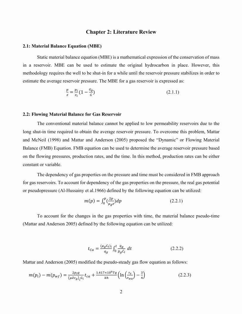
The dependency of gas properties on the pressure and time must be considered in FMB approach

for gas reservoirs. To account for dependency of the gas properties on the pressure, the real gas potential

or pseudopressure (Al-Hussainy et al.1966) defined by the following equation can be utilized: 𝑓𝑓(𝑝𝑝) = ∫ ( 2𝑝𝑝

𝜇𝜇𝑔𝑔𝑧𝑧)𝑝𝑝𝑝𝑝𝑝𝑝

0 (2.2.1)

To account for the changes in the gas properties with time, the material balance pseudo-time

(Mattar and Anderson 2005) defined by the following equation can be utilized:

𝑓𝑓𝐶𝐶𝑤𝑤 = (𝜇𝜇𝑔𝑔𝐶𝐶𝑡𝑡)𝑖𝑖

𝑞𝑞𝑔𝑔∫

𝑞𝑞𝑔𝑔𝜇𝜇�𝑔𝑔𝐶𝐶𝑝𝑡𝑡

𝑡𝑡0 𝑝𝑝𝑓𝑓 (2.2.2)

Mattar and Anderson (2005) modified the pseudo-steady gas flow equation as follows: 𝑓𝑓(𝑝𝑝𝑔𝑔) −𝑓𝑓(𝑝𝑝𝑤𝑤𝑓𝑓) = 2𝑝𝑝𝑖𝑖𝑞𝑞

�𝜇𝜇𝜇𝜇𝑐𝑐𝑔𝑔�𝑖𝑖𝐺𝐺𝑖𝑖𝑓𝑓𝑐𝑐𝑤𝑤 + 1.417×106𝑇𝑇𝑞𝑞

𝑘𝑘ℎ�ln � 𝑟𝑟𝑒𝑒

𝑟𝑟𝑤𝑤𝑤𝑤� − 3

4� (2.2.3)

3

And defined ba,pss as: 𝑏𝑏𝑤𝑤,𝑝𝑝𝑝𝑝𝑝𝑝 = 1.417×106𝑇𝑇

𝑘𝑘ℎ�ln � 𝑟𝑟𝑒𝑒

𝑟𝑟𝑤𝑤𝑤𝑤� − 3

4� (2.2.4)

Therefore equation 2.2.3 becomes:

𝑚𝑚(𝑝𝑝𝑖𝑖)−𝑚𝑚(𝑝𝑝𝑤𝑤𝑤𝑤)

𝑞𝑞= 2𝑝𝑝𝑖𝑖

�𝜇𝜇𝜇𝜇𝑐𝑐𝑔𝑔�𝑖𝑖𝐺𝐺𝑖𝑖𝑓𝑓𝑐𝑐𝑤𝑤 + 𝑏𝑏𝑤𝑤,𝑝𝑝𝑝𝑝𝑝𝑝 (2.2.5)

According to equation 2.2.5, a plot of 𝑚𝑚

(𝑝𝑝𝑖𝑖)−𝑚𝑚(𝑝𝑝𝑤𝑤𝑤𝑤)𝑞𝑞

𝑔𝑔𝑔𝑔𝑔𝑔𝑓𝑓𝑓𝑓𝑔𝑔𝑓𝑓 𝑓𝑓𝑐𝑐𝑤𝑤 will yield a straight-line where:

𝑆𝑆𝑣𝑣𝑓𝑓𝑝𝑝𝑣𝑣 = 2𝑝𝑝𝑖𝑖(𝑢𝑢𝑧𝑧𝑐𝑐𝑡𝑡)𝑖𝑖∗𝐺𝐺𝑖𝑖

(2.2.6)

𝐼𝐼𝑓𝑓𝑓𝑓𝑣𝑣𝑓𝑓𝑓𝑓𝑣𝑣𝑝𝑝𝑓𝑓 = 𝑏𝑏𝑤𝑤,𝑝𝑝𝑝𝑝𝑝𝑝 = 1.417×106𝑇𝑇𝑘𝑘ℎ

�ln � 𝑟𝑟𝑒𝑒𝑟𝑟𝑤𝑤𝑤𝑤� − 3

4� (2.2.7)

The following steps describe how the conventional flowing material balance can be applied:

1. Convert pi and 𝑝𝑝𝑤𝑤𝑓𝑓 to pseudopressure

2. Assume a value for the initial gas in place value (G).

3. Calculate 𝑝𝑝𝑧𝑧 for each cumulative gas production using Equation 2.1.1

4. Determine the average reservoir pressure, p, corresponding to 𝑝𝑝𝑧𝑧 value.

5. Determine gas viscosity and compressibility at the average reservoir pressure.

6. Determine the material balance pseudo-time using Equation 2.2.2.

7. Plot 𝑚𝑚(𝑝𝑝𝑖𝑖)−𝑚𝑚(𝑝𝑝𝑤𝑤𝑤𝑤)

𝑞𝑞 𝑔𝑔𝑔𝑔𝑔𝑔𝑓𝑓𝑓𝑓𝑔𝑔𝑓𝑓 𝑓𝑓𝑐𝑐𝑤𝑤 and draw a straight line through the points.

8. The gas in place can be calculated from Equation 2.2.6

9. Repeat steps 4-8 until the assumed and the calculated values of the initial gas in place converge.

2.3: King Method

Gregory King (1993) developed a new MBE to account for the presence of adsorbed gas in shale

and coalbed methane reservoirs. This MBE is given by equation 2.3.1:

𝑝𝑝𝑧𝑧∗

= 𝑝𝑝𝑖𝑖𝑧𝑧𝑖𝑖∗ (1 − 𝐺𝐺𝑝𝑝

𝐺𝐺) (2.3.1)

Where:

𝑧𝑧∗ = 𝑧𝑧

�1−𝑐𝑐𝑤𝑤�∗(𝑝𝑝𝑖𝑖−𝑝𝑝)∗(1−𝑆𝑆𝑤𝑤)+𝜌𝜌𝑏𝑏∗𝐵𝐵𝑔𝑔

𝜃𝜃 ∗�𝑉𝑉𝐿𝐿∗𝑝𝑝𝑃𝑃𝐿𝐿+𝑝𝑝� (2.3.2)

4

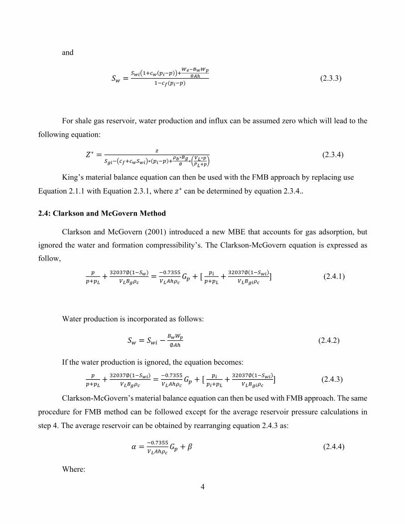
and

𝑆𝑆𝑤𝑤 =𝑆𝑆𝑤𝑤𝑖𝑖�1+𝑐𝑐𝑤𝑤(𝑝𝑝𝑖𝑖−𝑝𝑝)�+

𝑊𝑊𝑒𝑒−𝐵𝐵𝑤𝑤𝑊𝑊𝑝𝑝𝜃𝜃𝜃𝜃ℎ

1−𝑐𝑐𝑤𝑤(𝑝𝑝𝑖𝑖−𝑝𝑝) (2.3.3)

For shale gas reservoir, water production and influx can be assumed zero which will lead to the

following equation:

𝑍𝑍∗ = 𝑧𝑧

𝑆𝑆𝑔𝑔𝑖𝑖−�𝑐𝑐𝑤𝑤+𝑐𝑐𝑤𝑤𝑆𝑆𝑤𝑤𝑖𝑖�∗(𝑝𝑝𝑖𝑖−𝑝𝑝)+𝜌𝜌𝑏𝑏∗𝐵𝐵𝑔𝑔

𝜃𝜃 ∗�𝑉𝑉𝐿𝐿∗𝑝𝑝𝑃𝑃𝐿𝐿+𝑝𝑝� (2.3.4)

King’s material balance equation can then be used with the FMB approach by replacing use

Equation 2.1.1 with Equation 2.3.1, where 𝑧𝑧∗ can be determined by equation 2.3.4..

2.4: Clarkson and McGovern Method

Clarkson and McGovern (2001) introduced a new MBE that accounts for gas adsorption, but

ignored the water and formation compressibility’s. The Clarkson-McGovern equation is expressed as

follow,

𝑝𝑝𝑝𝑝+𝑝𝑝𝐿𝐿

+ 32037∅(1−𝑆𝑆𝑤𝑤)𝑉𝑉𝐿𝐿𝐵𝐵𝑔𝑔𝜌𝜌𝑐𝑐

= −0.7355𝑉𝑉𝐿𝐿𝐴𝐴ℎ𝜌𝜌𝑐𝑐

𝐺𝐺𝑝𝑝 + [ 𝑝𝑝𝑖𝑖𝑝𝑝+𝑝𝑝𝐿𝐿

+ 32037∅(1−𝑆𝑆𝑤𝑤𝑖𝑖)𝑉𝑉𝐿𝐿𝐵𝐵𝑔𝑔𝑖𝑖𝜌𝜌𝑐𝑐

] (2.4.1)

Water production is incorporated as follows:

𝑆𝑆𝑤𝑤 = 𝑆𝑆𝑤𝑤𝑔𝑔 −𝐵𝐵𝑤𝑤𝑊𝑊𝑝𝑝

∅𝐴𝐴ℎ (2.4.2)

If the water production is ignored, the equation becomes: 𝑝𝑝

𝑝𝑝+𝑝𝑝𝐿𝐿+ 32037∅(1−𝑆𝑆𝑤𝑤𝑖𝑖)

𝑉𝑉𝐿𝐿𝐵𝐵𝑔𝑔𝜌𝜌𝑐𝑐= −0.7355

𝑉𝑉𝐿𝐿𝐴𝐴ℎ𝜌𝜌𝑐𝑐𝐺𝐺𝑝𝑝 + [ 𝑝𝑝𝑖𝑖

𝑝𝑝𝑖𝑖+𝑝𝑝𝐿𝐿+ 32037∅(1−𝑆𝑆𝑤𝑤𝑖𝑖)

𝑉𝑉𝐿𝐿𝐵𝐵𝑔𝑔𝑖𝑖𝜌𝜌𝑐𝑐] (2.4.3)

Clarkson-McGovern’s material balance equation can then be used with FMB approach. The same

procedure for FMB method can be followed except for the average reservoir pressure calculations in

step 4. The average reservoir can be obtained by rearranging equation 2.4.3 as:

𝛼𝛼 = −0.7355𝑉𝑉𝐿𝐿𝐴𝐴ℎ𝜌𝜌𝑐𝑐

𝐺𝐺𝑝𝑝 + 𝛽𝛽 (2.4.4)

Where:

5

𝛼𝛼 = 𝑝𝑝𝑝𝑝+𝑝𝑝𝐿𝐿

+ 32037∅(1−𝑆𝑆𝑤𝑤𝑤𝑤)𝑉𝑉𝐿𝐿𝐵𝐵𝑔𝑔𝜌𝜌𝑐𝑐

(2.4.5)

𝛽𝛽 = 𝑝𝑝𝑤𝑤𝑝𝑝𝑤𝑤+𝑝𝑝𝐿𝐿

+ 32037∅(1−𝑆𝑆𝑤𝑤𝑤𝑤)𝑉𝑉𝐿𝐿𝐵𝐵𝑔𝑔𝑤𝑤𝜌𝜌𝑐𝑐

(2.4.6)

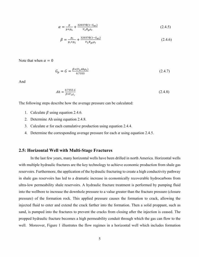
Note that when 𝛼𝛼 = 0

𝐺𝐺𝑝𝑝 = 𝐺𝐺 = 𝛽𝛽×(𝑉𝑉𝐿𝐿𝐴𝐴ℎ𝜌𝜌𝑐𝑐)0.7355

(2.4.7)

And

𝐴𝐴ℎ = 0.7355 𝐺𝐺𝛽𝛽×𝑉𝑉𝐿𝐿𝜌𝜌𝑐𝑐

(2.4.8)

The following steps describe how the average pressure can be calculated:

1. Calculate 𝛽𝛽 using equation 2.4.6.

2. Determine Ah using equation 2.4.8.

3. Calculate 𝛼𝛼 for each cumulative production using equation 2.4.4.

4. Determine the corresponding average pressure for each 𝛼𝛼 using equation 2.4.5.

2.5: Horizontal Well with Multi-Stage Fractures

In the last few years, many horizontal wells have been drilled in north America. Horizontal wells

with multiple hydraulic fractures are the key technology to achieve economic production from shale gas

reservoirs. Furthermore, the application of the hydraulic fracturing to create a high conductivity pathway

in shale gas reservoirs has led to a dramatic increase in economically recoverable hydrocarbons from

ultra-low permeability shale reservoirs. A hydraulic fracture treatment is performed by pumping fluid

into the wellbore to increase the downhole pressure to a value greater than the fracture pressure (closure

pressure) of the formation rock. This applied pressure causes the formation to crack, allowing the

injected fluid to enter and extend the crack farther into the formation. Then a solid proppant, such as

sand, is pumped into the fractures to prevent the cracks from closing after the injection is ceased. The

propped hydraulic fracture becomes a high permeability conduit through which the gas can flow to the

well. Moreover, Figure 1 illustrates the flow regimes in a horizontal well which includes formation

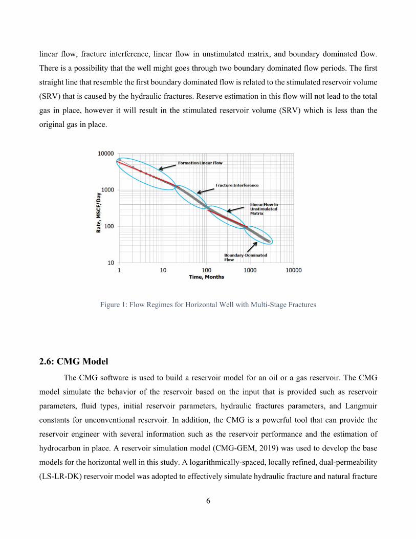
6

linear flow, fracture interference, linear flow in unstimulated matrix, and boundary dominated flow.

There is a possibility that the well might goes through two boundary dominated flow periods. The first

straight line that resemble the first boundary dominated flow is related to the stimulated reservoir volume

(SRV) that is caused by the hydraulic fractures. Reserve estimation in this flow will not lead to the total

gas in place, however it will result in the stimulated reservoir volume (SRV) which is less than the

original gas in place.

Figure 1: Flow Regimes for Horizontal Well with Multi-Stage Fractures

2.6: CMG Model

The CMG software is used to build a reservoir model for an oil or a gas reservoir. The CMG

model simulate the behavior of the reservoir based on the input that is provided such as reservoir

parameters, fluid types, initial reservoir parameters, hydraulic fractures parameters, and Langmuir

constants for unconventional reservoir. In addition, the CMG is a powerful tool that can provide the

reservoir engineer with several information such as the reservoir performance and the estimation of

hydrocarbon in place. A reservoir simulation model (CMG-GEM, 2019) was used to develop the base

models for the horizontal well in this study. A logarithmically-spaced, locally refined, dual-permeability

(LS-LR-DK) reservoir model was adopted to effectively simulate hydraulic fracture and natural fracture

7

behavior. The dual permeability model was selected to incorporate the naturally fractured nature of

shales, and the logarithmic refinement was required to capture the transient effects around the hydraulic

fracture. Evenly spaced gridding would allow for the fine gridding required around the fracture, but it

would not create unnecessary grid refinement far away from the fracture. The dual-permeability model

accounts for the flow that can occur in the natural fractures, in the matrix, and from the natural fracture

to matrix.

8

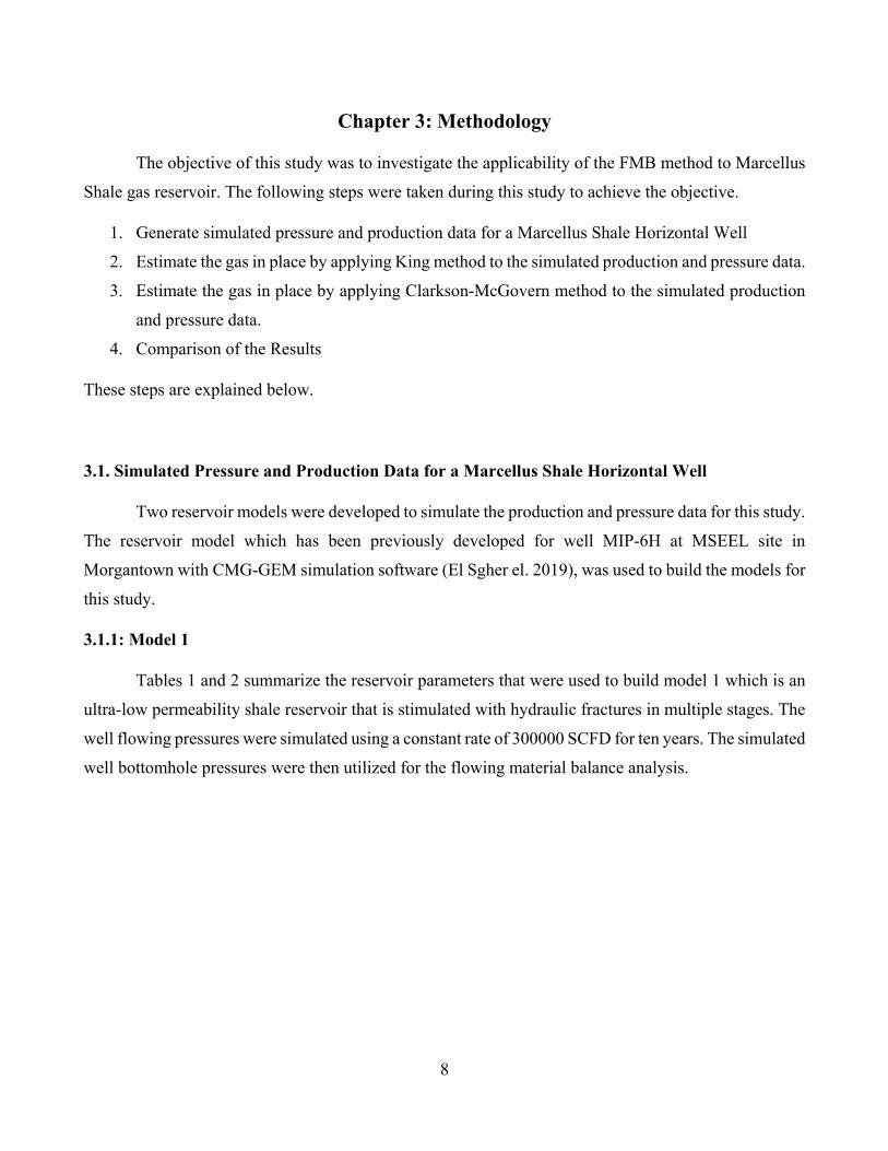
Chapter 3: Methodology

The objective of this study was to investigate the applicability of the FMB method to Marcellus

Shale gas reservoir. The following steps were taken during this study to achieve the objective.

1. Generate simulated pressure and production data for a Marcellus Shale Horizontal Well

2. Estimate the gas in place by applying King method to the simulated production and pressure data.

3. Estimate the gas in place by applying Clarkson-McGovern method to the simulated production

and pressure data.

4. Comparison of the Results

These steps are explained below.

3.1. Simulated Pressure and Production Data for a Marcellus Shale Horizontal Well

Two reservoir models were developed to simulate the production and pressure data for this study.

The reservoir model which has been previously developed for well MIP-6H at MSEEL site in

Morgantown with CMG-GEM simulation software (El Sgher el. 2019), was used to build the models for

this study.

3.1.1: Model 1

Tables 1 and 2 summarize the reservoir parameters that were used to build model 1 which is an

ultra-low permeability shale reservoir that is stimulated with hydraulic fractures in multiple stages. The

well flowing pressures were simulated using a constant rate of 300000 SCFD for ten years. The simulated

well bottomhole pressures were then utilized for the flowing material balance analysis.

9

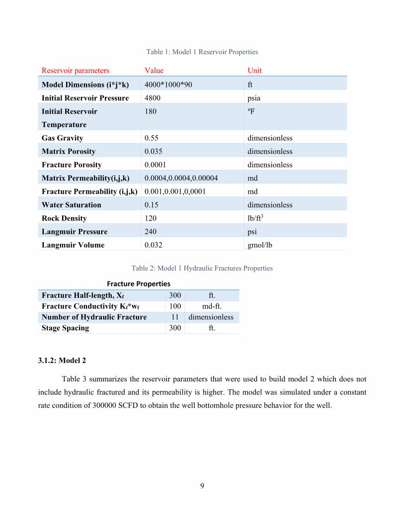
Table 1: Model 1 Reservoir Properties

Reservoir parameters Value Unit

Model Dimensions (i*j*k) 4000*1000*90 ft

Initial Reservoir Pressure 4800 psia

Initial Reservoir

Temperature

180 ℉

Gas Gravity 0.55 dimensionless

Matrix Porosity 0.035 dimensionless

Fracture Porosity 0.0001 dimensionless

Matrix Permeability(i,j,k) 0.0004,0.0004,0.00004 md

Fracture Permeability (i,j,k) 0.001,0.001,0,0001 md

Water Saturation 0.15 dimensionless

Rock Density 120 lb/ft3

Langmuir Pressure 240 psi

Langmuir Volume 0.032 gmol/lb

Table 2: Model 1 Hydraulic Fractures Properties

Fracture Properties Fracture Half-length, Xf 300 ft. Fracture Conductivity Kf*wf 100 md-ft. Number of Hydraulic Fracture 11 dimensionless Stage Spacing 300 ft.

3.1.2: Model 2

Table 3 summarizes the reservoir parameters that were used to build model 2 which does not

include hydraulic fractured and its permeability is higher. The model was simulated under a constant

rate condition of 300000 SCFD to obtain the well bottomhole pressure behavior for the well.

10

Table 3: Model 2 Reservoir Properties

Reservoir parameters Value Unit

Model Dimensions (i*j*k) 4000*1000*90 ft

Initial Reservoir Pressure 4800 psia

Initial Reservoir

Temperature

180 ℉

Gas Gravity 0.55 dimensionless

Matrix Porosity 0.035 dimensionless

Fracture Porosity 0.0001 dimensionless

Matrix Permeability(i,j,k) 0.1,0.1,0.01 md

Fracture Permeability (i,j,k) 0.001,0.001,0,0001 md

Water Saturation 0.15 dimensionless

Rock Density 120 lb/ft3

Langmuir Pressure 240 psi

Langmuir Volume 0.032 gmol/lb

3.2. Gas in Place Estimation by the Conventional FMB

A spreadsheet model was developed to estimate the gas in place following the steps outlined in

Chapter 2 for the conventional FMB method. The spreadsheet model included several routines to

determine gas deviation factor, gas viscosity, gas compressibility, pseudopressure, and the material

balance pseudo-time based on the gas gravity, reservoir temperature, and the average reservoir pressure.

3.3. Gas in Place Estimation by the King Method

A spreadsheet model was developed to estimate the gas in place following the steps outlined in

Chapter 2 for the King’s method. The spreadsheet model included several routines to determine gas

deviation factor as described by Equation 2.3.4, gas viscosity, gas compressibility, pseudopressure, and

the material balance pseudo-time based on the gas gravity, reservoir temperature, and the average

reservoir pressure.

11

3.4. Gas in Place Estimation by the Clarkson-McGovern Method

A spreadsheet model was developed to estimate the gas in place following the steps outlined in

Chapter 2 for the Clarkson-McGovern method. The spreadsheet model included several routines to

determine gas deviation factor, gas viscosity, gas compressibility, pseudopressure, and the material

balance pseudo-time based on the gas gravity, reservoir temperature, and the average reservoir pressure.

12

Chapter 4: Results and Discussion

4.1: Model 1 Results

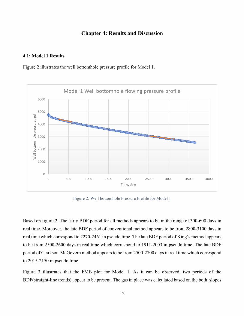
Figure 2 illustrates the well bottomhole pressure profile for Model 1.

Figure 2: Well bottomhole Pressure Profile for Model 1

Based on figure 2, The early BDF period for all methods appears to be in the range of 300-600 days in

real time. Moreover, the late BDF period of conventional method appears to be from 2800-3100 days in

real time which correspond to 2270-2461 in pseudo time. The late BDF period of King’s method appears

to be from 2500-2600 days in real time which correspond to 1911-2003 in pseudo time. The late BDF

period of Clarkson-McGovern method appears to be from 2500-2700 days in real time which correspond

to 2015-2150 in pseudo time.

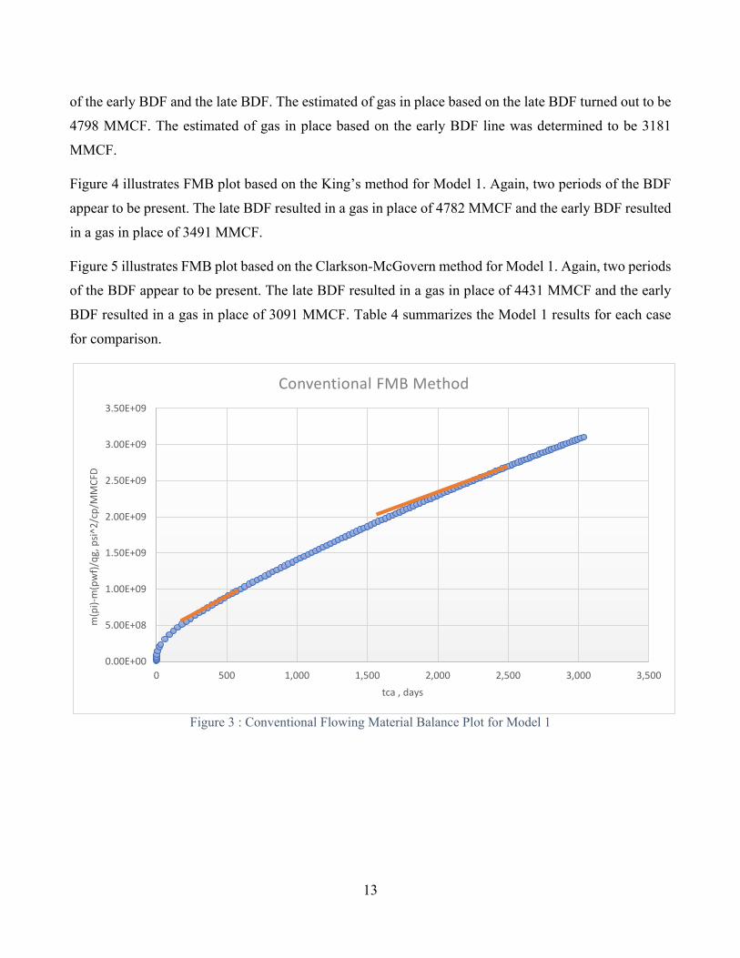
Figure 3 illustrates that the FMB plot for Model 1. As it can be observed, two periods of the

BDF(straight-line trends) appear to be present. The gas in place was calculated based on the both slopes

0

1000

2000

3000

4000

5000

6000

0 500 1000 1500 2000 2500 3000 3500 4000

Wel

l bot

tom

hol

e pr

essu

re ,

psi

Time, days

Model 1 Well bottomhole flowing pressure profile

13

of the early BDF and the late BDF. The estimated of gas in place based on the late BDF turned out to be

4798 MMCF. The estimated of gas in place based on the early BDF line was determined to be 3181

MMCF.

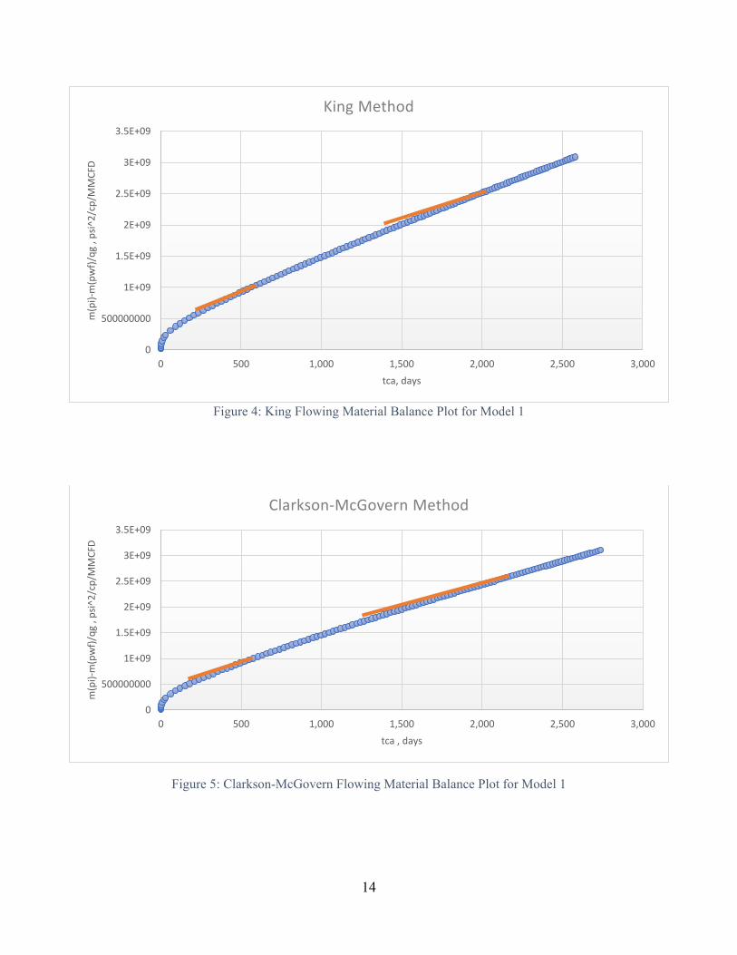
Figure 4 illustrates FMB plot based on the King’s method for Model 1. Again, two periods of the BDF

appear to be present. The late BDF resulted in a gas in place of 4782 MMCF and the early BDF resulted

in a gas in place of 3491 MMCF.

Figure 5 illustrates FMB plot based on the Clarkson-McGovern method for Model 1. Again, two periods

of the BDF appear to be present. The late BDF resulted in a gas in place of 4431 MMCF and the early

BDF resulted in a gas in place of 3091 MMCF. Table 4 summarizes the Model 1 results for each case

for comparison.

Figure 3 : Conventional Flowing Material Balance Plot for Model 1

0.00E+00

5.00E+08

1.00E+09

1.50E+09

2.00E+09

2.50E+09

3.00E+09

3.50E+09

0 500 1,000 1,500 2,000 2,500 3,000 3,500

m(p

i)-m

(pw

f)/qg

, psi^

2/cp

/MM

CFD

tca , days

Conventional FMB Method

14

Figure 4: King Flowing Material Balance Plot for Model 1

Figure 5: Clarkson-McGovern Flowing Material Balance Plot for Model 1

0

500000000

1E+09

1.5E+09

2E+09

2.5E+09

3E+09

3.5E+09

0 500 1,000 1,500 2,000 2,500 3,000

m(p

i)-m

(pw

f)/qg

, ps

i^2/

cp/M

MCF

D

tca , days

Clarkson-McGovern Method

0

500000000

1E+09

1.5E+09

2E+09

2.5E+09

3E+09

3.5E+09

0 500 1,000 1,500 2,000 2,500 3,000

m(p

i)-m

(pw

f)/qg

, ps

i^2/

cp/M

MCF

D

tca, days

King Method

15

Table 4: Comparison of the Results for Model 1

Gas in Place, Early BDF

MMCF

Gas in Place, Late BDF ,MMCF

Method

CMG Model 2006 4304

Conventional FMB 3181 4798

King Method 3491 4782

Clarkson-McGovern Method 3091 4431

4.2: Model 2 Results

Figure 6 illustrates the well bottomhole pressure profile for Model 2.

Figure 6: Well bottomhole Pressure Profile for Model 2

0

1000

2000

3000

4000

5000

6000

0 500 1000 1500 2000 2500 3000 3500 4000

pwf ,

psi

Time ,days

Model 2 : Well bottomhole pressure profile

16

Based on figure 6, The BDF period for the conventional and Clarkson-McGovern methods appears to

be in the range of 1700-3600 days in real time which correspond to 1530-3000 days in pseudo time. The

BDF period for the King’s method appears to be from 2500-2600 days in real time which correspond to

2057-2140 in pseudo time.

Figure 7 illustrates that the FMB plot for Model 2. As it can be observed, one period of BDF(straight-

line trends) appears to be present. The gas in place was calculated based on the slope of the BDF. The

estimated of gas in place based on the BDF turned out to be 4565 MMCF.

Figure 8 illustrates FMB plot based on the King’s method for Model 2. Again, one period of the BDF

appears to be present. The BDF resulted in a gas in place of 4782 MMCF.

Figure 9 illustrates FMB plot based on the Clarkson-McGovern method for Model 2. Again, one period

of the BDF appears to be present.The BDF resulted in a gas in place of 4433 MMCF. Table 5 summarizes

the Model 2 results for each case for comparison.

Figure 7: Conventional Flowing Material Balance Plot for Model 2

0.00E+00

5.00E+08

1.00E+09

1.50E+09

2.00E+09

2.50E+09

3.00E+09

3.50E+09

0 500 1000 1500 2000 2500 3000 3500

m(p

i)-m

(pw

f)/qg

, ps

i^2/

cp/M

MCF

D

tca ,days

Conventional FMB Method

17

Figure 8: King Flowing Material Balance Plot for Model 2

Figure 9: Clarkson-McGovern Flowing Material Balance Plot for Model 2

0

500000000

1E+09

1.5E+09

2E+09

2.5E+09

3E+09

3.5E+09

0 500 1000 1500 2000 2500 3000 3500

m(p

i)-m

(pw

f)/qg

, psi^

2/cp

/MM

CFD

tca, days

King Method

0.00E+00

5.00E+08

1.00E+09

1.50E+09

2.00E+09

2.50E+09

3.00E+09

3.50E+09

0 500 1000 1500 2000 2500 3000 3500

m(p

i)-m

(pw

f)/qg

, ps

i^2/

cp/M

MCF

D

tca, days

Clarkson-McGovern Method

18

Table 5: Comparison of the Results for Model 2

Gas in Place ,MMCF

Method

CMG Model 4304

Conventional FMB 4565

King Method 4782

Clarkson-McGovern Method 4433

19

Chapter 5: Conclusion and Recommendations

This conclusions were reached in this study

1. Two boundary dominated flow (BDF) periods may be present for a hydraulically fractured gas

reservoir with ultra-low permeability (Model 1).

2. The early BDF may provide the estimate of the gas in place for the stimulated reservoir volume

(SRV).

3. The late BDF can provide the estimate of the gas in place for the entire reservoir.

4. Clarkson-McGovern method provided the most accurate predictions of the gas in place, for both

SRV and the total gas for Model 1.

5. Only one BDF period appears to be present for the low-permeability reservoir without hydraulic

fracture (Model 2) which can be used to estimate the total gas in place.

6. Clarkson-McGovern method provided the most accurate prediction of the gas in place for the

total gas in place for Model 2.

It is recommended that additional case (Models) to be considered to further investigate the impact of

the number and properties of the hydraulic fractures, the gas adsorption parameters, and the formation

properties on the application of FMB to ultra-low permeability reservoirs.

20

References

Han, G., Liu, M., & Li, Q. (2020). Flowing material balance method with adsorbed phase volumes for

unconventional gas reservoirs. Energy Exploration & Exploitation, 38(2), 519-532.

Moghadam, S., Jeje, O., & Mattar, L. (2011). Advanced gas material balance in simplified

format. Journal of Canadian Petroleum Technology, 50(01), 90-98.

Mattar, L., & Anderson, D. (2005, January). Dynamic material balance (oil or gas-in-place without shut-

ins). In Canadian International Petroleum Conference. Petroleum Society of Canada.

King, G. R. (1993). Material-balance techniques for coal-seam and devonian shale gas reservoirs with

limited water influx. SPE Reservoir Engineering, 8(01), 67-72.

Clarkson, C.R. and McGovern, J.M. (2001) Study of the Potential Impact of Matrix Free Gas Storage

Upon Coalbed Gas Reserves and Production Using a New Material Balance Equation. Paper

0113, Proceedings of the 2001 International Coalbed Methane Symposium, The University of

Alabama, Tuscaloosa, Alabama, p. 133-149.

Williams-Kovacs, J.D., Clarkson, C.R., , Nobakht, M.,(2012), Impact of Material Balance Equation

Selection on Rate-Transient Analysis of Shale Gas. SPE 158041

Morad , K., & Clarkson, C. R. (2006). Application of Flowing P/z* Material Balance for Dry Coalbed-

Methane Reservoirs . Society of Petroleum Engineers .

Mattar , L., & McNeil, R. (1998). The "Flowing" Gas Maerial Balance . Petroleum Society of Canada

Agarwal, R. G., Gardner, D. C., Kleinsteiber, S. W., & Fussell, D. D. (1998). Analyzing Well Production

Data Using Combined Type Curve and Decline Curve Analysis Concepts

El Sgher, M., Aminian, K., & Ameri, S. (2019, October 15). The Impact of Rock Properties and Stress

Shadowing on the Hydraulic Fracture Properties in Marcellus Shale. Society of Petroleum

Engineers. doi:10.2118/196590-MS