Application of Design of Experiment to a Gas Turbine ... · Testing of gas turbine blades within a specialized, well-understood, test cell environment remains a key part of the overall

1 Copyright © 2013 by ASME

Proceedings of GT2013 ASME Turbo Expo 2013: Power for Land, Sea and Air

June 3-7, 2013, San Antonio, USA

GT2013-94314

Application of Design of Experiment to a Gas Turbine Cascade Test Cell

R O Evans1, W N Dawes2 & Q Zhang3 1Cambridge Flow Solutions Ltd, Compass House, Vision Park, Cambridge UK,

2Whittle Laboratory, Cambridge University Engineering Department, Cambridge UK 3University of Michigan-Shanghai Jiao Tong University Joint Institute,

Shanghai Jiao Tong University, Shanghai, China.

ABSTRACT

Testing of gas turbine blades within a specialized, well-understood, test cell environment remains a key part of the overall design process. This paper describes the simulation of a cascade of transonic turbine blades within the full test cell environment. The objective of this simulation is to bring CFD to bear to understand various installation issues which go into the design of the test cell. The focus here is on the role of the tailboards in managing periodic test conditions in a cascade with relatively few blades and transonic exit. Using a Design of Experiment methodology a series of simulations was performed with a systematic variation in both the location of solid tailboards and the open area ratio of a slotted tailboard. The flow relative to the target test blade was successfully optimized with respect to a reference periodic condition. INTRODUCTION For the CFD simulation to produce reliable, useful data a range of scales needs to be covered and the full complexity of the geometry confronted. At the micro-scale are the blades themselves, typically installed in a cascade in a working section with some sort of tailboard and associated instrumentation. At the meso-scale is the integration of the working section within a test chamber with the associated risks of distorted boundary conditions. At the macro-scale is the overall performance of the test cell: inlet flow smoothness to the test chamber, start-up transients, balancing Mach number & Reynolds number against pressure level and power consumption. The design and commissioning of a successful test environment represents a significant engineering challenge.

Fig.1: Overview and CAD model of the turbine cascade test cell (courtesy Shanghai Jiao Tong

University/University of Michigan Joint Institute) . In this paper we show the first-of-a-kind simulation of a full test cell environment, Figure 1, demonstrating how the power of CFD can be brought to bear on this challenge. In particular the role of the tailboards in managing a periodic flow for the test blade is studied. Gostelow [1] described the main approaches to managing periodicity in transonic cascade testing. The


first is simply to have no tailboard (ie. “open jet”) – but blade exit shocks waves reflect from the free shear layer as strong expansion waves and poor periodicity can result. A solid tailboard can be used as the expansion ratio of the exit flow can be controlled by careful tuning of the tailboard angles – but the blade exit shocks can reflect (as shocks now) and again can interfere with periodicity. Following standard transonic wind tunnel testing practice, tailboards that are porous or slotted can also be used. Here the idea is that impinging blade exit shocks will partially reflect as expansions from free shear layers in the open area portions of the tailboard and cancel the shocks reflected from the closed area portions. McFarland [2] provides an up-to-date review of this topic. Accordingly, in this paper two studies are reported using a Design of Experiment methodology varying first the positioning of suction and pressure side solid tailboards and then, second, the open area ratio of a slotted tailboard. In both cases the aim is to optimize the tailboard geometry to achieve the best periodicity with respect to the test blade. SETTING UP THE SIMULATION

Geometry & Meshing The key bottleneck in attempting such an ambitious simulation is generating a mesh for the extensive and very complex geometry; an overview and CAD model of the rig is shown in Figure 1. Over recent years a series of papers (Dawes et al [3-8]) have described a step-change in mesh generating capability based on the radically different approach to both geometry and mesh generation which has grown up to support physics-based animation in the film and computer games industry – see for example Baerentzen [9] and Galyean et al [10] and the annual SIGGRAPH Conference series. The key to this approach is to adopt an implicit geometry model rather than the more conventional explicit approach (for example: NURBS patches, edges and topology bindings). The implicit model represents the geometry by a distance field, captured on an octree and managed as a Level Set (see Adalsteinsson et al [11] for example). This allows great freedom as the geometry can then be handled as a scalar variable, can support a variety of Boolean operations (allowing geometry to be “added” or “subtracted” for example) – and parallelised trivially. The main disadvantage is that the geometry does not need to be strictly quantitative for the purposes of animation. However, for scientific or engineering simulation the geometry must be faithfully represented. The geometry and meshing system produced as a result of our research, BoXeR [12], is a scriptable, automatable system capable of dealing with true

geometry and overcoming all the disadvantages of the conventional approaches to mesh generation (as, for example, surveyed comprehensively at the annual International Meshing Roundtable: Shontz [13]). The meshing system consists of five stages; each of which required substantial technical innovation: 1. The first stage captures the geometry digitally (like

a 3D photograph) via a dynamically load balanced bottom-up octree based on very efficient space filling curve technology (the traditional top-down octree is difficult to implement in parallel); this background mesh supports the imported geometry as a solid model using distance fields managed as a Level Set

2. Next, a conjugate body-conformal hybrid mesh is constructed using shape insertion, to allow the octree to better match the body curvature, followed by snapping to the actual surface; the key technology here is mesh smoothing driven by a series of mesh quality metrics (skew, warpage, cell-to-cell variation, etc.)

3. Viscous layer meshes are then inserted using the distance field as a guide – formally the gradient of the distance field is the surface normal and so issues like geometry corners or geometry proximity are much easier to manage

4. Active feature detection for sharp corners and for thin/zero thickness geometries is required as the geometry is held implicitly; this makes use of local mesh topology swapping and smoothing

5. Finally all of the algorithms are implemented in parallel - including most of the i/o using HDF5 – so that scalability to massive problem sizes is straightforward and automatic.

More detail can be found in reference [3-8].

Application to the test rig

Application of our geometry and meshing system to the UM-SJTU turbine test rig shown earlier in Figure 1 is a routine task. The entire rig was meshed with ~50M cells by importing direct the manufacturing CAD - with no need for cleaning or de-featuring - in a wall-clock time of about half an hour. A wide range of scales is resolved – the blade itself is resolved down to Y+~O(10) – even the details of the upstream honeycomb flow straighteners are resolved similarly.

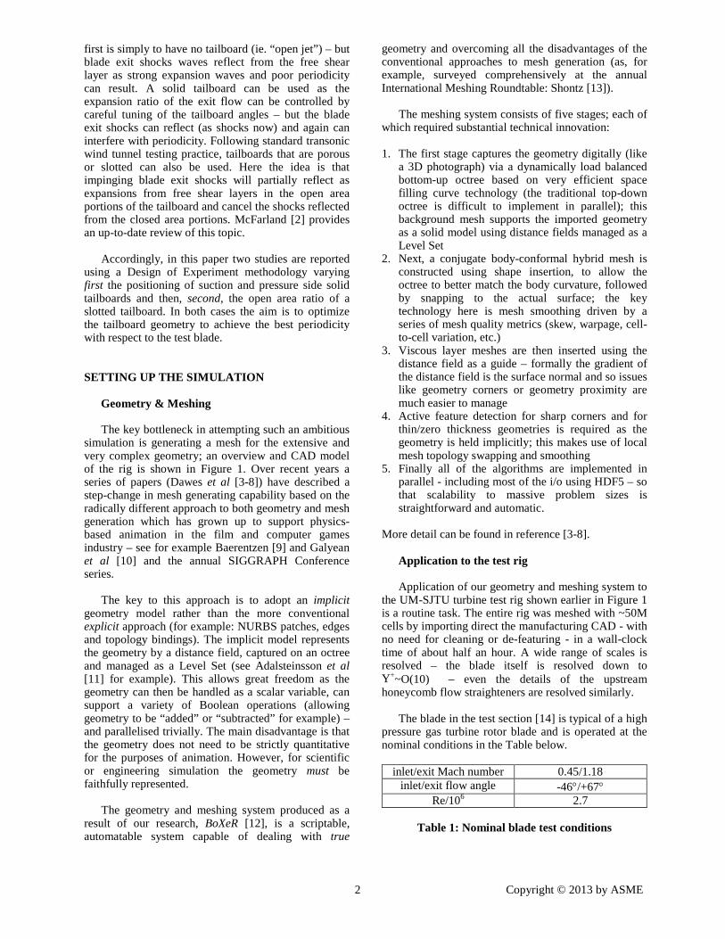
The blade in the test section [14] is typical of a high

pressure gas turbine rotor blade and is operated at the nominal conditions in the Table below.

inlet/exit Mach number 0.45/1.18

inlet/exit flow angle -46°/+67° Re/106 2.7

Table 1: Nominal blade test conditions


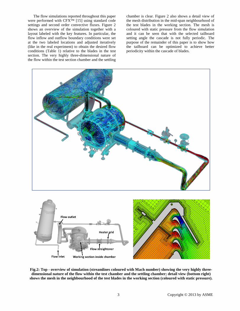
The flow simulations reported throughout this paper were performed with CFX™ [15] using standard code settings and second order convective fluxes. Figure 2 shows an overview of the simulation together with a layout labeled with the key features. In particular, the flow inflow and outflow boundary conditions were set at the two labeled locations and adjusted iteratively (like in the real experiment) to obtain the desired flow conditions (Table 1) relative to the blades in the test section. The very highly three-dimensional nature of the flow within the test section chamber and the settling

chamber is clear. Figure 2 also shows a detail view of the mesh distribution in the mid-span neighbourhood of the test blades in the working section. The mesh is coloured with static pressure from the flow simulation and it can be seen that with the selected tailboard setting angle the cascade is not fully periodic. The purpose of the remainder of this paper is to show how the tailboard can be optimized to achieve better periodicity within the cascade of blades.

Fig.2: Top - overview of simulation (streamlines coloured with Mach number) showing the very highly three-dimensional nature of the flow within the test chamber and the settling chamber; detail view (bottom right)

shows the mesh in the neighbourhood of the test blades in the working section (coloured with static pressure).


OPTIMIZATION via DESIGN of EXPERIMENT

Preamble

A simulation which integrated the geometry management, meshing & CFD would allow the tailboards to be quickly adjusted or modified to maximize periodicity. This can formally be set up as a classical optimization problem, simplified to a Design of Experiment (DoE). The following sections will discuss in turn the building blocks which need to be assembled into an integrated workflow to achieve this.

Design of Experiment The cost of CFD simulation has motivated the

search for low order (or surrogate or meta) models to replace the CFD where it can. The basis of low order modeling is to maintain a list of k design parameters with corresponding objective functions and to fit to them some sort of k-dimensional surface or other lower order model. This list usually is derived initially from some sort of Design of Experiment and subsequently can be populated with the accumulated simulations to date. Very good discussion on this can be found in Keane et al [16].

The heart of the Design of Experiment methodology

is to choose an appropriate variation in each of the design parameters so that the design space is effectively populated and, hopefully, illuminated. This choice of parameter variation can be based on a variety of approaches ranging from uniform or random sampling to Taguchi orthogonal or 2n factorial sampling or even more sophisticated, and statistically based, Latin Hypercube or LP-τ sequences. The main motivation for this is to try to characterize a design space defined by a large number of parameters with as few expensive function evaluations as possible. However, in the work reported here the number of design parameters is relatively few – the main challenge is the complexity of the geometry and the need to automate the DoE (especially the mesh generation) - so for simplicity full factorial sampling was adopted.

The DoE then proceeds by performing a flow simulation for each combination of parameters and then fitting a low order model to the resulting variation in objective function. This can then be used to choose the optimum set of design parameters. This low order model can be a Response Surface of various orders (including least square) or more sophisticated methods like Kriging or Neural Networks which are “trained” to fit the data (via auxiliary optimization). More detail is given in Keane et al [16]. In this work, for simplicity, a piecewise linear Response Surface was chosen.

Objective function The next building block is to define the objective

function to be optimized. Here we are focused on

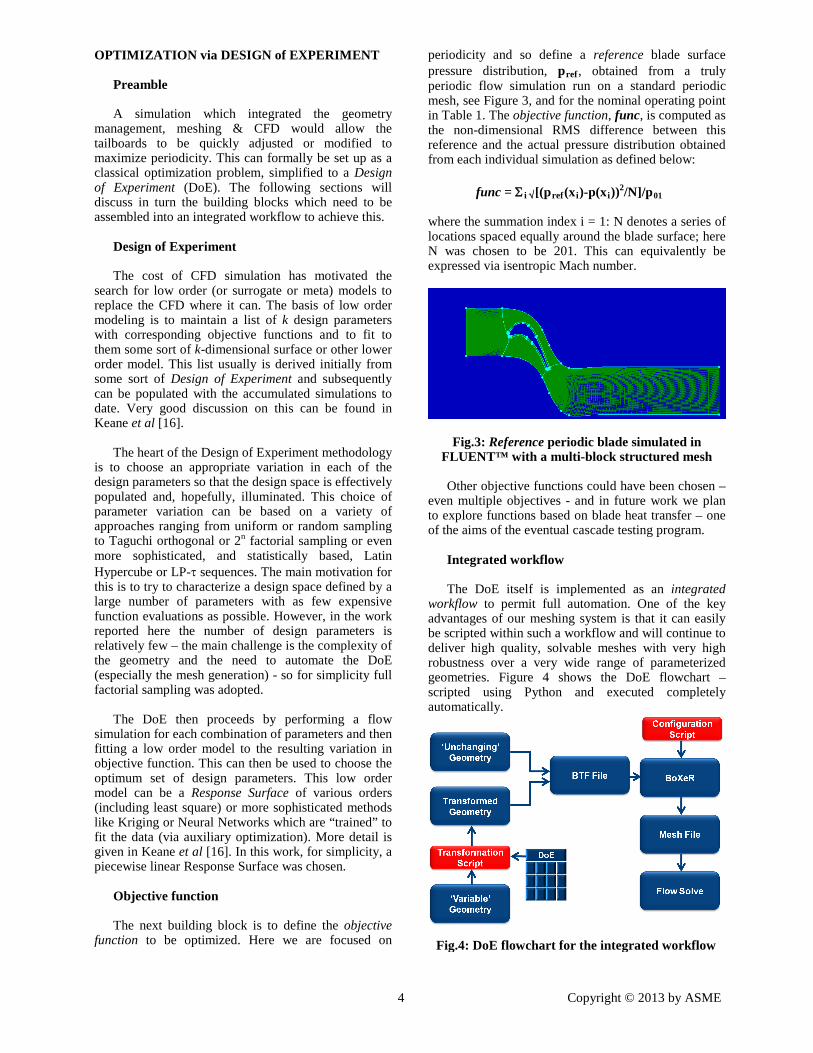
periodicity and so define a reference blade surface pressure distribution, pref, obtained from a truly periodic flow simulation run on a standard periodic mesh, see Figure 3, and for the nominal operating point in Table 1. The objective function, func, is computed as the non-dimensional RMS difference between this reference and the actual pressure distribution obtained from each individual simulation as defined below:

func = Σ i √[(pref(xi)-p(xi))2/N]/p01

where the summation index i = 1: N denotes a series of locations spaced equally around the blade surface; here N was chosen to be 201. This can equivalently be expressed via isentropic Mach number.

Fig.3: Reference periodic blade simulated in FLUENT™ with a multi-block structured mesh

Other objective functions could have been chosen –

even multiple objectives - and in future work we plan to explore functions based on blade heat transfer – one of the aims of the eventual cascade testing program.

Integrated workflow The DoE itself is implemented as an integrated

workflow to permit full automation. One of the key advantages of our meshing system is that it can easily be scripted within such a workflow and will continue to deliver high quality, solvable meshes with very high robustness over a very wide range of parameterized geometries. Figure 4 shows the DoE flowchart – scripted using Python and executed completely automatically.

Fig.4: DoE flowchart for the integrated workflow


Flow simulation

The flow simulations were performed using CFX integrated via standard scripting within the workflow in Figure 4. The boundary conditions were set to obtain the nominal blade operating conditions given in Table 1. Each successive simulation was initialized with the previous one as initial guess.

Parameterisation Last but not least is the parameterisation - which

for this study consisted of two parts: variable locations for the suction and pressure side tailboards and open area ratio for a slotted tailboard. The geometry variations were handled and managed by importing the geometry, via named CAD parts, into the geometry kernel of our meshing system and then scripting their locations and configurations. In a virtual sense this is just like how the real geometry is managed in the real test rig.

More detail is presented in the following sections.

RESULTS and DISCUSSION

Tailboard angles

Figure 5 shows the computational domain and range of movement for the tailboards. There were 8 pressure side positions and 7 suction side positions in the DoE leading to 56 cases run.

Fig.5: Computational domain and range of movement for tailboards; the DoE consisted of 8 PS positions x 7 SS positions = 56 cases run

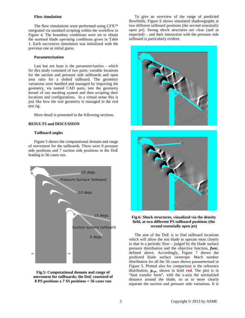
To give an overview of the range of predicted flowfields, Figure 6 shows simulated shadowgraphs at two different tailboard positions (the second essentially open jet). Strong shock structures are clear (and as expected) – and their interaction with the pressure side tailboard is particularly evident.

Fig.6: Shock structures, visualized via the density field, at two different PS tailboard positions (the

second essentially open jet)

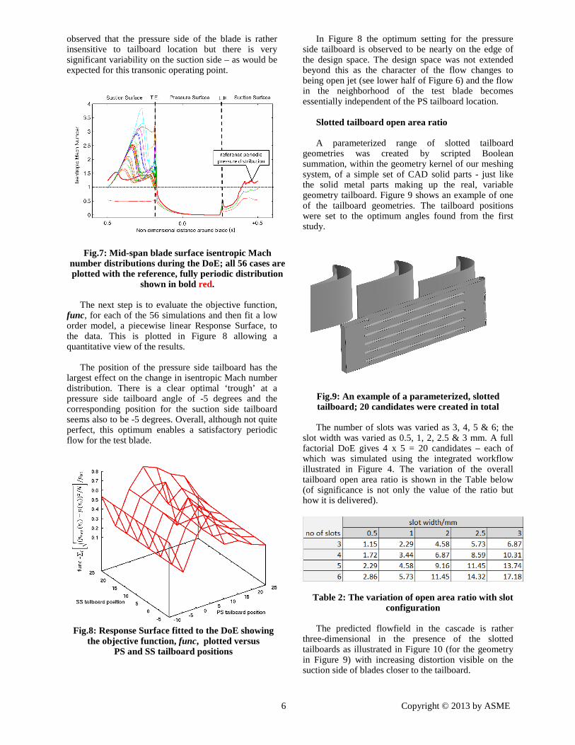
The aim of the DoE is to find tailboard locations which will allow the test blade to operate most closely to that in a periodic flow – judged by the blade surface pressure distribution and the objective function, func, defined above. Accordingly, Figure 7 shows the predicted blade surface isentropic Mach number distribution for all the 56 cases shown parameterised in Figure 5. Plotted also for comparison is the reference distribution, pref, shown in bold red. The plot is in “heat transfer form”, with the x-axis the normalised distance around the blade, so as to more clearly separate the suction and pressure side variations. It is


observed that the pressure side of the blade is rather insensitive to tailboard location but there is very significant variability on the suction side – as would be expected for this transonic operating point.

Fig.7: Mid-span blade surface isentropic Mach number distributions during the DoE; all 56 cases are plotted with the reference, fully periodic distribution

shown in bold red.

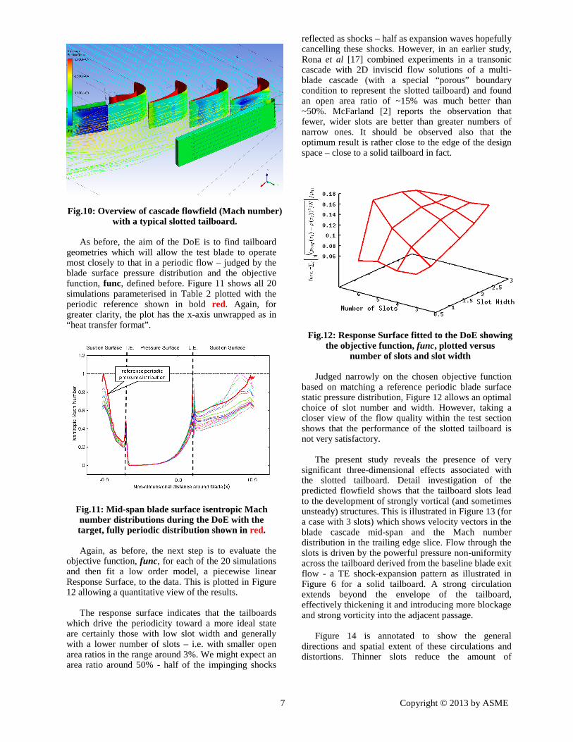
The next step is to evaluate the objective function, func, for each of the 56 simulations and then fit a low order model, a piecewise linear Response Surface, to the data. This is plotted in Figure 8 allowing a quantitative view of the results.

The position of the pressure side tailboard has the

largest effect on the change in isentropic Mach number distribution. There is a clear optimal ‘trough’ at a pressure side tailboard angle of -5 degrees and the corresponding position for the suction side tailboard seems also to be -5 degrees. Overall, although not quite perfect, this optimum enables a satisfactory periodic flow for the test blade.

Fig.8: Response Surface fitted to the DoE showing

the objective function, func, plotted versus PS and SS tailboard positions

In Figure 8 the optimum setting for the pressure side tailboard is observed to be nearly on the edge of the design space. The design space was not extended beyond this as the character of the flow changes to being open jet (see lower half of Figure 6) and the flow in the neighborhood of the test blade becomes essentially independent of the PS tailboard location.

Slotted tailboard open area ratio

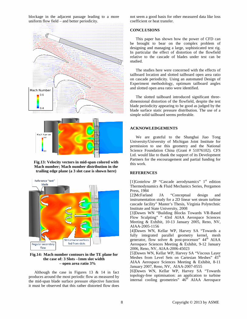
A parameterized range of slotted tailboard

geometries was created by scripted Boolean summation, within the geometry kernel of our meshing system, of a simple set of CAD solid parts - just like the solid metal parts making up the real, variable geometry tailboard. Figure 9 shows an example of one of the tailboard geometries. The tailboard positions were set to the optimum angles found from the first study.

Fig.9: An example of a parameterized, slotted tailboard; 20 candidates were created in total

The number of slots was varied as 3, 4, 5 & 6; the

slot width was varied as 0.5, 1, 2, 2.5 & 3 mm. A full factorial DoE gives 4 x 5 = 20 candidates – each of which was simulated using the integrated workflow illustrated in Figure 4. The variation of the overall tailboard open area ratio is shown in the Table below (of significance is not only the value of the ratio but how it is delivered).

Table 2: The variation of open area ratio with slot configuration

The predicted flowfield in the cascade is rather

three-dimensional in the presence of the slotted tailboards as illustrated in Figure 10 (for the geometry in Figure 9) with increasing distortion visible on the suction side of blades closer to the tailboard.


Fig.10: Overview of cascade flowfield (Mach number) with a typical slotted tailboard.

As before, the aim of the DoE is to find tailboard

geometries which will allow the test blade to operate most closely to that in a periodic flow – judged by the blade surface pressure distribution and the objective function, func, defined before. Figure 11 shows all 20 simulations parameterised in Table 2 plotted with the periodic reference shown in bold red. Again, for greater clarity, the plot has the x-axis unwrapped as in “heat transfer format”.

Fig.11: Mid-span blade surface isentropic Mach number distributions during the DoE with the target, fully periodic distribution shown in red.

Again, as before, the next step is to evaluate the

objective function, func, for each of the 20 simulations and then fit a low order model, a piecewise linear Response Surface, to the data. This is plotted in Figure 12 allowing a quantitative view of the results.

The response surface indicates that the tailboards

which drive the periodicity toward a more ideal state are certainly those with low slot width and generally with a lower number of slots – i.e. with smaller open area ratios in the range around 3%. We might expect an area ratio around 50% - half of the impinging shocks

reflected as shocks – half as expansion waves hopefully cancelling these shocks. However, in an earlier study, Rona et al [17] combined experiments in a transonic cascade with 2D inviscid flow solutions of a multi-blade cascade (with a special “porous” boundary condition to represent the slotted tailboard) and found an open area ratio of ~15% was much better than ~50%. McFarland [2] reports the observation that fewer, wider slots are better than greater numbers of narrow ones. It should be observed also that the optimum result is rather close to the edge of the design space – close to a solid tailboard in fact.

Fig.12: Response Surface fitted to the DoE showing the objective function, func, plotted versus

number of slots and slot width

Judged narrowly on the chosen objective function based on matching a reference periodic blade surface static pressure distribution, Figure 12 allows an optimal choice of slot number and width. However, taking a closer view of the flow quality within the test section shows that the performance of the slotted tailboard is not very satisfactory.

The present study reveals the presence of very

significant three-dimensional effects associated with the slotted tailboard. Detail investigation of the predicted flowfield shows that the tailboard slots lead to the development of strongly vortical (and sometimes unsteady) structures. This is illustrated in Figure 13 (for a case with 3 slots) which shows velocity vectors in the blade cascade mid-span and the Mach number distribution in the trailing edge slice. Flow through the slots is driven by the powerful pressure non-uniformity across the tailboard derived from the baseline blade exit flow - a TE shock-expansion pattern as illustrated in Figure 6 for a solid tailboard. A strong circulation extends beyond the envelope of the tailboard, effectively thickening it and introducing more blockage and strong vorticity into the adjacent passage.

Figure 14 is annotated to show the general

directions and spatial extent of these circulations and distortions. Thinner slots reduce the amount of


blockage in the adjacent passage leading to a more uniform flow field – and better periodicity.

Fig.13: Velocity vectors in mid-span colored with Mach number; Mach number distribution in the trailing edge plane (a 3 slot case is shown here)

Fig.14: Mach number contours in the TE plane for

the case of: 3 Slots –1mm slot width – open area ratio 3%

Although the case in Figures 13 & 14 in fact

produces around the most periodic flow as measured by the mid-span blade surface pressure objective function it must be observed that this rather distorted flow does

not seem a good basis for other measured data like loss coefficient or heat transfer. CONCLUSIONS

This paper has shown how the power of CFD can be brought to bear on the complex problem of designing and managing a large, sophisticated test rig. In particular the effect of distortion of the flowfield relative to the cascade of blades under test can be studied.

The studies here were concerned with the effects of

tailboard location and slotted tailboard open area ratio on cascade periodicity. Using an automated Design of Experiment methodology, optimum tailboard angles and slotted open area ratio were identified.

The slotted tailboard introduced significant three-

dimensional distortion of the flowfield, despite the test blade periodicity appearing to be good as judged by the blade surface static pressure distribution. The use of a simple solid tailboard seems preferable.

ACKNOWLEDGEMENTS

We are grateful to the Shanghai Jiao Tong University/University of Michigan Joint Institute for permission to use this geometry and the National Science Foundation China (Grant # 51076102). CFS Ltd. would like to thank the support of its Development Partners for the encouragement and partial funding for this work. REFERENCES [1]Gostelow JP “Cascade aerodynamics” 1st edition Thermodynamics & Fluid Mechanics Series, Pergamon Press, 1984 [2]McFarland JA “Conceptual design and instrumentation study for a 2D linear wet steam turbine cascade facility” Master’s Thesis, Virginia Polytechnic Institute and State University, 2008 [3]Dawes WN “Building Blocks Towards VR-Based Flow Sculpting” ” 43rd AIAA Aerospace Sciences Meeting & Exhibit, 10-13 January 2005, Reno, NV, AIAA-2005-1156 [4]Dawes WN, Kellar WP, Harvey SA “Towards a fully integrated parallel geometry kernel, mesh generator, flow solver & post-processor” 44th AIAA Aerospace Sciences Meeting & Exhibit, 9-12 January 2006, Reno, NV, AIAA-2006-45023 [5]Dawes WN, Kellar WP, Harvey SA “Viscous Layer Meshes from Level Sets on Cartesian Meshes” 45th AIAA Aerospace Sciences Meeting & Exhibit, 8-11 January 2007, Reno, NV, AIAA-2007-0555 [6]Dawes WN, Kellar WP, Harvey SA “Towards topology-free optimisation: an application to turbine internal cooling geometries” 46th AIAA Aerospace


Sciences Meeting & Exhibit, 7-10 January 2008, Reno, NV, AIAA-2008-925 [7]Dawes WN, Kellar WP, Harvey SA ”A practical demonstration of scalable parallel mesh generation” 47th AIAA Aerospace Sciences Meeting & Exhibit, 9-12 January 2009, Orlando, FL, AIAA-2009-0981 [8]Dawes WN, Kellar WP, Harvey SA “Generation of conjugate meshes for complex geometries for coupled multi-physics simulations” 87th AIAA Aerospace Sciences Meeting & Exhibit, 7-10 January 2010, Orlando, FL, AIAA-2010-062 [9]Baerentzen A “Volume sculpting: intuitive, interactive 3D shape modelling” IMM, May 2001 [10]Galyean TA & Hughes JF “Sculpting: an interactive volumetric modelling technique” ACM Trans., Computer Graphics, vol.25, no.4, pp 267-274, 1991 [11]Adalsteinsson D & Sethian JA “A level set approach to a unified model for etching, deposition & lithography II: three dimensional simulations” Journal of Comput.Phys, 122, 348-366, 1995 [12]www.cambridgeflowsolutions.com [13]Shontz S, Editor, Proceedings of the 19th International Meshing Roundtable, Chattanooga TN, 2010 [14]Thorpe S.J., Yoshino ,S., Ainsworth R.W., and Harvey N.W., “An investigation of the heat transfer and static pressure on the over-tip casing wall of an axial turbine operating at engine representative flow conditions. (I). Time-mean results.” International Journal of Heat and Fluid Flow 25 (2004) 933–944 [15]www.ansys.com [16]Keane AJ & Nair PB “Computational Approaches for Aerospace Design: The Pursuit of Excellence” John Wiley & Sons, June 2005 [17]Rona A, Paciorri R, Geron M & Ince NZ “Slot width augmentation in a slotted-wall transonic linear cascade wind tunnel” 42nd AIAA Aerospace Sciences Meeting & Exhibit, Reno, 2004

-oOo-

http://www.ansys.com/

Documents

Application of Design of Experiment to a Gas Turbine ... · Testing of gas turbine blades within a specialized, well-understood, test cell environment remains a key part of the overall