Application of density-based propagation to fragment

Application of density-based propagation to fragment clouds using the Starling suite

S. Frey(1), C. Colombo(1), and S. Lemmens(2)

(1)Politecnico di Milano, Via La Masa 34, 20156 Milano, Italy, stefan.frey/[email protected](2)Space Debris Office, ESA/ESOC, Robert-Bosch-Strasse 5, 64293 Darmstadt, Germany; [email protected]

ABSTRACT

The Starling suite estimates the non-linear evolution of densities in orbit. These densities can be probability densityfunctions describing uncertainties about states or distributions of particle clouds modeled as continua. In this work, theStarling suite is applied to satellite fragmentations in a circular as well as highly eccentric orbit around Earth. Theformer case is challenging because the fragment distribution is bounded. Such boundedness is tackled using featurespaces defined relative to propagated reference hypersurfaces. The latter case is challenging as assumptions of therandomization in the node and argument of perigee do not hold over the mid-term. The suite also allows to estimate theimpact rate from a fragment cloud on missions in any orbital region. Estimating the consequences of fragmentations isimportant as it can be used to rate planned space missions in terms of risks towards the future space environment.

1 INTRODUCTION

More than 500 on-orbit fragmentations have so far occurred due to various reasons including explosions andcollisions [1]. Explosions of spacecraft and upper stages and collisions with other objects potentially release hundredsof thousands of fragments with a diameter larger than 1 mm [2]. To estimate the long-term consequences of suchfragment clouds on active space missions in terms of impact rates and collision risk, a diverse set of tools weredeveloped. Engineering tools, such as NASA’s LEGEND [3], rely on Monte Carlo sampling to estimate the number ofcollisions from space debris. They are non-invasive and thus work with any existing propagator in any force model fora wide range of orbit geometries. However, to derive an accurate density estimate in 6+ dimensions over the fulldomain requires a prohibitively large number of samples to be drawn and propagated. Other tools directly propagatedensities through volume mapping [4] or application of the continuum equation [5]. Their analyticalimplementations [6] require simplified force models and restricted orbital geometries. Numerical solutions [7, 8, 9] candeal with any dynamics but the result is known only following the characteristics of the system. Solutions based onfinite-differences [10, 11, 12, 13], instead, model the distribution over the full domain but are difficult to extend intomore than 3 dimensions due to restrictions in terms of computational power and memory. Hence, a method combiningthe best of all worlds to be fast, applicable for many force models and orbital geometries and extendable into manydimensions is desirable.

Here, a novel tool, the Starling suite, is introduced to estimate evolving continua subject to non-linear dynamics. Thesuite is being developed at the Politecnico di Milano and funded by the COMPASS European Research Council projectand the European Space Agency. The name is inspired by the murmurations of starlings, a spectacle of nature wheremillions of birds fly together in perfect synchrony, seemingly as one ever-changing continuum. It is based on thecontinuity equation and uses numerical propagation to allow incorporation of accurate force models and modeling ofdensities in any orbit. To estimate the distribution across the full domain without requiring a large number ofpropagations, Starling fits a surrogate model to the characteristics. The suite was designed to allow working in anydimensionality and with easy transitioning between feature spaces. An additional plug-in estimates the rate of impactsan evolving fragment cloud has on targets in any orbital regime. Two examples of fragmentation cloud evolution aregiven in 2 and 5 dimensions, respectively. The former shows the usage of reference hypersurfaces to normalize thefeature space and facilitate the fitting of the surrogate model. It also shows the application of the impact rate estimationtool. The later shows the potential of the method of propagating clouds in many dimensions while keeping thecomputational resources required low.

This work is organized as follows: Sec. 2 and 3 give an overview of the theoretical background of the method anddiscuss limitations. The tool itself is described in Sec. 4. Use cases of the tool, propagation of a fragment clouds andestimation of the collision risk, are presented in Sec. 5. Finally, conclusions are drawn in Sec. 6.

6089.pdfFirst Int'l. Orbital Debris Conf. (2019)

2 CONTINUUM FORMULATIONThe uncertainty and/or fragment cloud distribution are modeled as density functions. Uncertainties are probabilitydensity functions, i.e. integration over the full domain results in unity. Fragment distributions, instead, are particledensity functions. Integration over the full domain results in the number of fragments, N , that are present in the cloud.The method presented here does not distinguish between the two types of densities, and both are simply referred to asdensity function, nxxx, in the D-dimensional phase space, xxx ∈ RD.

The following subsections discuss the initial condition and transformation (Sec. 2.1), the propagation of the continuum(Sec. 2.2), how to find surrogate models at different snapshots in the future (Sec. 2.3), as well as current limitations tothe approach (Sec. 2.4).

2.1 Init ial distribution and transformationHere, the main focus lies in the long-term propagation of fragmentation clouds. To speed up the integration of thetrajectories, the particles are propagated in averaged orbital elements. The initial condition is required to be given in thesame element set. Often, however, the initial distribution is not given in the appropriate phase space. The initialfragment distribution given by the NASA standard breakup model (SBM) [2] is defined as a function of the magnitudeof the velocity, ∆v, relative to the parent orbit, and fragment characteristics, bbbT = (L A/m), with the characteristiclength, L, and the area-to-mass ratio, A/m. The distribution, nvvv,bbb, that can be obtained from the NASA SBM is definedin the velocity, vvv ∈ R3, and bbb, and can be extended to include uncertainties also in radial direction, rrr [14].

For propagation, the distribution is transformed into Keplerian elements, αααT = (a e i Ω ω f), with the semi-majoraxis, a, the eccentricity, e, the inclination, i, the right ascension of ascending node, Ω, the argument of perigee, ω, andthe true anomaly, f . This can be achieved by application of the method of change of variables [15, 14] as

nααα,bbb =nsss,bbb(ϕϕϕ

−1(ααα))

|detJJJ | Jij =∂ϕi∂sj

(1)

with the point transformation, ϕϕϕ, from ααα to sssT = (rrrT vvvT ) and the Jacobian of the transformation, JJJ . Forsemi-analytical propagation, randomization of f is assumed.

2.2 Continuum propagationThe distribution is modeled as a continuum. To predict its evolution, the general continuity equation is applied [5]

∂nxxx∂t

+∇ · (nxxxFFF ) = 0dxxx

dt= FFF (2)

with the density, nxxx, given in the phase space, xxxT = (αααT bbbT ) ∈ RD in D dimensions, the independent variable time, t,the dynamics, FFF , and ignoring sources and sink terms. This partial differential equation can be converted into anordinary differential equation using the method of characteristics [5], giving an additional equation for the densityevolution

dnxxxdt

= −nxxx tr

(∂FFF

∂xxx

)(3)

with the trace, tr. The characteristics of the system follow the trajectories. They are propagated using the PlanODynsuite [16] as it provides the Jacobian of the averaged dynamics with respect to the mean elements for all the majorperturbations. The effect of drag is modeled according to [17]. The fragment characteristics, bbb, are assumed to beconstant.

The drawback of the method of the characteristics is that the solution to the equation is known only along thecharacteristics. To obtain the solution over the full domain, interpolation between the characteristics is required (seenext Subsection). The initial characteristics are selected through the Metropolis-Hastings algorithm [18], given theinitial NASA SBM distribution.

2.3 Surrogate modelingThe characteristics are propagated until the time or times of interest for evaluation of the number of impacts on activemissions. At each of these snapshots, a Gaussian Mixture Model (GMM) [19] is fitted to the characteristics in order to


obtain a fast to evaluate surrogate model. Please see Ref. [9] for an in depth discussion of the fitting procedure, which isbased on the minimization of a cost function.

If the underlying distribution exhibits strongly non-linear behavior, fitting a GMM might not be computationallypractical as a large number of kernels is required. Furthermore, the breakup distribution can exhibit boundedness (e.g.eccentricity is bounded to be positive). The problem is tackled by introducing one or multiple reference hyperplanes,defined through samples that are propagated using the same force model as the characteristics. A continuous definitionof the hyperplane is found through interpolation of the reference samples. The cloud characteristics are then fitted in the∆-space, e.g. in the ∆e = e− er, where er is the reference hyperplane. As the reference samples are subject to thesame non-linear deformations as the cloud characteristics, the resulting ∆-space shows less non-linear behavior and isthus easier to fit using a small number of kernels. Sec. 5 explains the concept using examples.

2.4 Current l imitat ions

The method was successfully tested on a large number of orbital configurations, in varying dimensions subject toatmospheric drag and the oblateness of Earth (J2), albeit neglecting the J2-drag coupling.

At this stage, the method is not suitably able to accommodate forces that lead to resonances on a small subset of thefeature space. Perturbations from third bodies or solar radiation pressure potentially induce resonances. Suchresonances tend to separate, or branch out, parts of the distribution from the main bulk of the characteristics.Additionally, it renders the reference hypersurfaces to be a function of all the elements rather than just a few decoupledones. This introduces inaccuracies in the definition of the surfaces and hence leads to faulty ∆-space distributions.

Currently, the possibility of performing domain splitting [20] for the cases where the distribution branches out andprohibits convergence of the fitting is investigated. If the branch can be isolated and separated such that both the branchand the remaining samples can be well represented in their respective subdomains, the GMMs could be fitted separately.

3 IMPACT ESTIMATION

For mid- to long-term propagation, assumptions can be made on the distribution of LEO fragmentations after a certainamount of time [21]. Shortly after the fragmentation, given even small differences in the orbit energy and area-to-massratio, the fragments will randomize over the mean anomaly, M , and form a torus. After a few years and due to theoblateness of the Earth, the fragments will further distribute into a band, i.e. randomize in both Ω and ω and limited inlatitude by the parent inclination, i0, which is assumed to be constant.

These assumptions can be used if the distribution in the full Keplerian element set, nααα, is to be recovered from asimpler definition in less elements. Note that in this section the dependence on the fragment characteristics, bbb, isdropped for better readability. It can either be integrated out, or carried through along the derivations to get an impactrate dependent on the fragment characteristic.

If the distribution is given as a function of the spatial variables a and e only, the dependence on i can be recovered byassuming a fixed i = i0 for all fragments, i.e.

na,e,i = δ(i− i0)na,e (4)

where δ is the Dirac delta function, defined as

δ(x) =

1, if x = 0

0, otherwise(5)

The dependence on the angles, Ω, ω, and M , is introduced by assuming uniform distribution over [0, 2π)

na,e,i,Ω,ω,M =1

(2π)3na,e,i (6)

Using the following transformations between M , eccentric anomaly, E, and f [22]

M = E − e sinE cosE =e+ cos f

1 + e cos fsinE =

√1− e2 sin f

1 + e cos f(7)


the derivative of f with respect to M is found as

df

dM=

(1 + e cos f)2

(1− e2)3/2(8)

Thus, the distribution in the full Keplerian elements set, ααα, using the method of change of variables as

nααα =

∣∣∣∣ df

dM

∣∣∣∣−1

na,e,i,Ω,ω,M =(1− e2)3/2

(1 + e cos f)2na,e,i,Ω,ω,M ∀f ∈ [0, 2π) (9)

To estimate the number of impacts, the distribution of fragments, nsss, in Cartesian coordinates, sss, is required. This canbe obtained by rearranging Eq. 1 as

nsss = |detJJJ |nααα (10)

The fragment density, nsss = nsss(rrr,vvv), is a function of both the radius, rrr, and velocity vvv. Integration over vvv yields thespatial density, nrrr, however, the directional information is important for the estimation of the impact rate. To calculatethe rate of impact, ni(rrr,vvv∗), at any given point in space and target velocity, vvv∗, integration of the product of thecross-sectional area, A, nsss and the magnitude of the relative velocity, ||∆vvv∗|| = ||vvv − vvv∗||, over all the fragmentvelocities is required

ni(rrr,vvv∗) =

∫ ∫ ∫A

(∆vvv∗

||∆vvv∗||

)nsss (rrr,vvv) ||∆vvv∗||dvvv (11)

where it is assumed that nsss is constant over A and that the area of the chaser is negligible compared to the target. If Ais independent of the direction of impact, i.e. if the target is a sphere, it can be taken out of the integration. If theinclination of the distribution is assumed constant, the volume integral reduces to two area integrals. Finally, thenumber of impacts can be calculated by integrating over time, t, as

ni(t) =

∫ t

t0

ni (rrr(t), vvv∗(t)) dt (12)

4 TOOL STRUCTURE

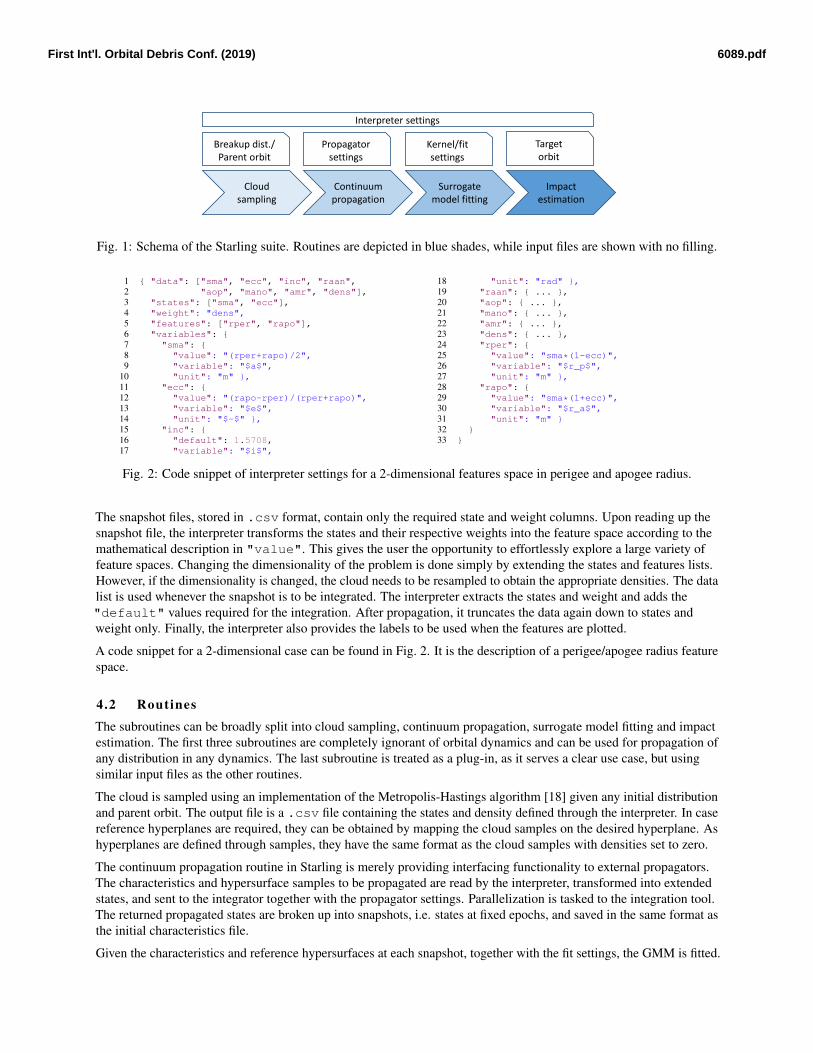
The Starling suite consists of several independent routines, which can be found in Fig. 1. The majority of the routines,shown in boxes with blue shades, are implemented in the PYTHON language. Input files, shown in boxes withtransparent background, are formatted as JSON or comma separated value files. The role of the interpreter that isrequired throughout all the subroutines is briefly introduced in Sec. 4.1. The subroutines and their respective inputs arediscussed in Sec. 4.2.

4.1 Interpreter

One of the main objectives of Starling is to seamlessly increase/decrease the dimensionality of the problem and switchbetween different feature spaces. The interpreter takes the role of understanding and transforming the characteristicsusing symbolic mathematics and the SYMPY package [23]. It is itself defined through the interpreter settings, a JSONfile containing

"variables": a dictionary of all the variables present, with the following items"value": symbolic representation of the feature as a function of the states"default": default value in case it is not part of the feature space but only used during integration"variable"/"unit": required for labeling of the figure axes

"data": list of strings describing the full element set, i.e. mix of values and default values required forintegration"states": list of strings describing subset of the data required for the feature space"weight": string describing the density around the state"features": list of strings describing features to be used for model fitting, defined through symbolicrepresentation as a function of the states


Continuum propagation

Surrogate model fitting

Impact estimation

Breakup dist./Parent orbit

Propagator settings

Kernel/fit settings

Target orbit

Interpreter settings

Cloud sampling

Fig. 1: Schema of the Starling suite. Routines are depicted in blue shades, while input files are shown with no filling.

1 "data": ["sma", "ecc", "inc", "raan",2 "aop", "mano", "amr", "dens"],3 "states": ["sma", "ecc"],4 "weight": "dens",5 "features": ["rper", "rapo"],6 "variables": 7 "sma": 8 "value": "(rper+rapo)/2",9 "variable": "$a$",

10 "unit": "m" ,11 "ecc": 12 "value": "(rapo-rper)/(rper+rapo)",13 "variable": "$e$",14 "unit": "$-$" ,15 "inc": 16 "default": 1.5708,17 "variable": "$i$",

18 "unit": "rad" ,19 "raan": ... ,20 "aop": ... ,21 "mano": ... ,22 "amr": ... ,23 "dens": ... ,24 "rper": 25 "value": "sma*(1-ecc)",26 "variable": "$r_p$",27 "unit": "m" ,28 "rapo": 29 "value": "sma*(1+ecc)",30 "variable": "$r_a$",31 "unit": "m" 32 33

Fig. 2: Code snippet of interpreter settings for a 2-dimensional features space in perigee and apogee radius.

The snapshot files, stored in .csv format, contain only the required state and weight columns. Upon reading up thesnapshot file, the interpreter transforms the states and their respective weights into the feature space according to themathematical description in "value". This gives the user the opportunity to effortlessly explore a large variety offeature spaces. Changing the dimensionality of the problem is done simply by extending the states and features lists.However, if the dimensionality is changed, the cloud needs to be resampled to obtain the appropriate densities. The datalist is used whenever the snapshot is to be integrated. The interpreter extracts the states and weight and adds the"default" values required for the integration. After propagation, it truncates the data again down to states andweight only. Finally, the interpreter also provides the labels to be used when the features are plotted.

A code snippet for a 2-dimensional case can be found in Fig. 2. It is the description of a perigee/apogee radius featurespace.

4.2 Routines

The subroutines can be broadly split into cloud sampling, continuum propagation, surrogate model fitting and impactestimation. The first three subroutines are completely ignorant of orbital dynamics and can be used for propagation ofany distribution in any dynamics. The last subroutine is treated as a plug-in, as it serves a clear use case, but usingsimilar input files as the other routines.

The cloud is sampled using an implementation of the Metropolis-Hastings algorithm [18] given any initial distributionand parent orbit. The output file is a .csv file containing the states and density defined through the interpreter. In casereference hyperplanes are required, they can be obtained by mapping the cloud samples on the desired hyperplane. Ashyperplanes are defined through samples, they have the same format as the cloud samples with densities set to zero.

The continuum propagation routine in Starling is merely providing interfacing functionality to external propagators.The characteristics and hypersurface samples to be propagated are read by the interpreter, transformed into extendedstates, and sent to the integrator together with the propagator settings. Parallelization is tasked to the integration tool.The returned propagated states are broken up into snapshots, i.e. states at fixed epochs, and saved in the same format asthe initial characteristics file.

Given the characteristics and reference hypersurfaces at each snapshot, together with the fit settings, the GMM is fitted.


Different snapshots can be fitted in parallel. The GMM is stored in a JSON file, including all the relevant informationto retrieve the full distribution. Additionally, a fit result file is stored containing information about the quality of the fit.

Lastly, the impact estimation tool, a separate plug-in to Starling, requires the GMM file, reference hypersurface samplesand a definition of the target orbit to calculate the number of impacts.

5 APPLICATION

Fragment clouds from two different orbital regions are presented. First, the initial fragment cloud of an explosion froma circular parent orbit is presented in 2 dimensions, in a feature space derived from a and e. The impact rate isestimated at different times, assuming a fixed parent inclination and randomization in all angles. This example strives tostrengthen the understanding of the usage of the reference hypersurface and shows the estimation of the impact rate.Second, the evolution of a fragment cloud of an explosion from a highly eccentric parent orbit is presented in5 dimensions, in a feature space derived from a, e, Ω, ω, and A/m. This example shows the potential of the continuumapproach in terms of computational efficiency in higher dimensions.

Both examples are modeled according to the NASA SBM [2] as a rocket body explosion considering characteristiclengths between 1 mm and 1 m, resulting in N0 = 3.8× 105 fragments.

5.1 Cloud evolution in 2 dimensions and impact rate est imation

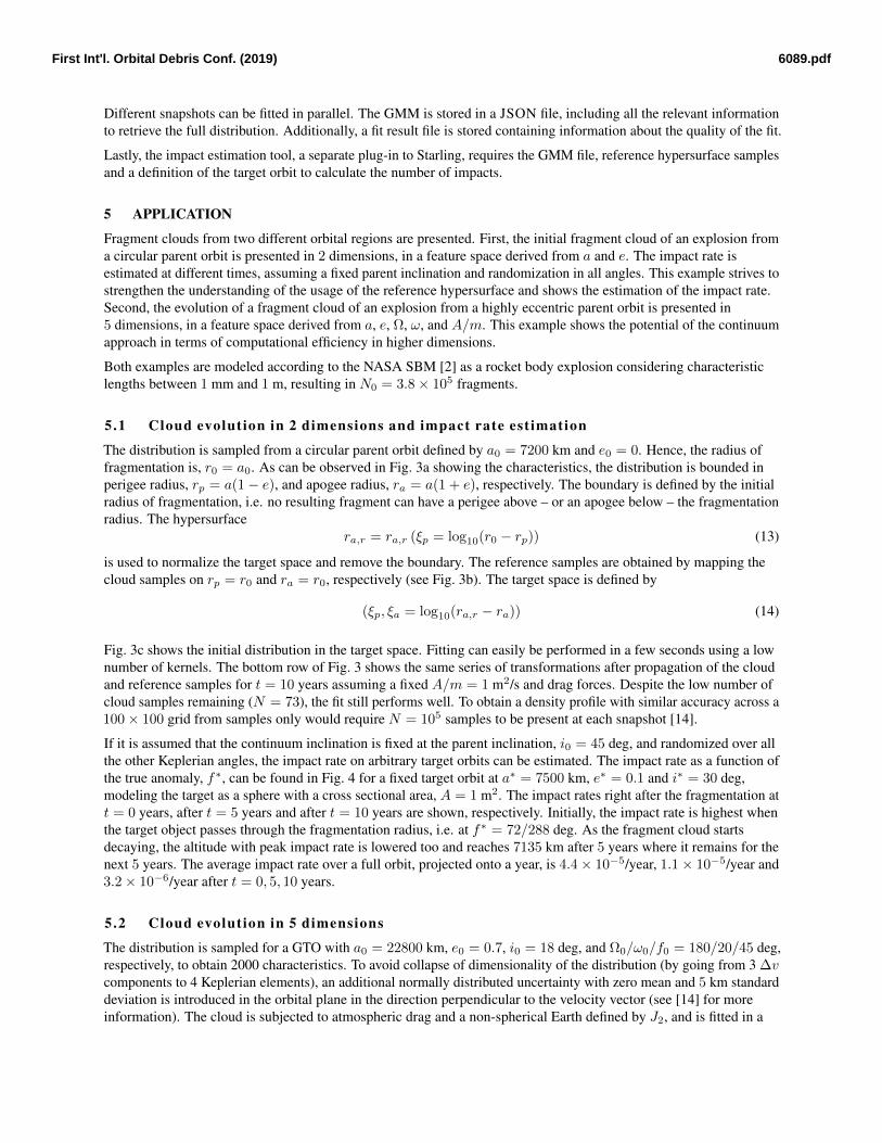
The distribution is sampled from a circular parent orbit defined by a0 = 7200 km and e0 = 0. Hence, the radius offragmentation is, r0 = a0. As can be observed in Fig. 3a showing the characteristics, the distribution is bounded inperigee radius, rp = a(1− e), and apogee radius, ra = a(1 + e), respectively. The boundary is defined by the initialradius of fragmentation, i.e. no resulting fragment can have a perigee above – or an apogee below – the fragmentationradius. The hypersurface

ra,r = ra,r (ξp = log10(r0 − rp)) (13)

is used to normalize the target space and remove the boundary. The reference samples are obtained by mapping thecloud samples on rp = r0 and ra = r0, respectively (see Fig. 3b). The target space is defined by

(ξp, ξa = log10(ra,r − ra)) (14)

Fig. 3c shows the initial distribution in the target space. Fitting can easily be performed in a few seconds using a lownumber of kernels. The bottom row of Fig. 3 shows the same series of transformations after propagation of the cloudand reference samples for t = 10 years assuming a fixed A/m = 1 m2/s and drag forces. Despite the low number ofcloud samples remaining (N = 73), the fit still performs well. To obtain a density profile with similar accuracy across a100× 100 grid from samples only would require N = 105 samples to be present at each snapshot [14].

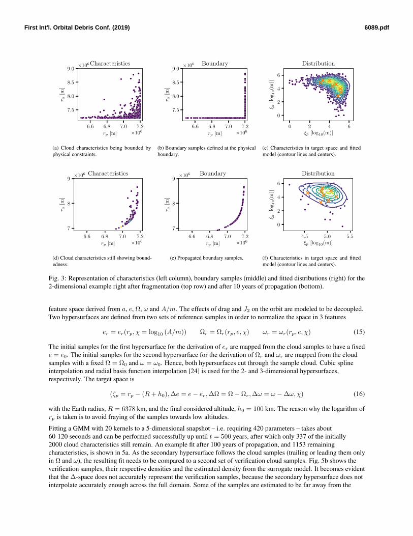
If it is assumed that the continuum inclination is fixed at the parent inclination, i0 = 45 deg, and randomized over allthe other Keplerian angles, the impact rate on arbitrary target orbits can be estimated. The impact rate as a function ofthe true anomaly, f∗, can be found in Fig. 4 for a fixed target orbit at a∗ = 7500 km, e∗ = 0.1 and i∗ = 30 deg,modeling the target as a sphere with a cross sectional area, A = 1 m2. The impact rates right after the fragmentation att = 0 years, after t = 5 years and after t = 10 years are shown, respectively. Initially, the impact rate is highest whenthe target object passes through the fragmentation radius, i.e. at f∗ = 72/288 deg. As the fragment cloud startsdecaying, the altitude with peak impact rate is lowered too and reaches 7135 km after 5 years where it remains for thenext 5 years. The average impact rate over a full orbit, projected onto a year, is 4.4× 10−5/year, 1.1× 10−5/year and3.2× 10−6/year after t = 0, 5, 10 years.

5.2 Cloud evolution in 5 dimensions

The distribution is sampled for a GTO with a0 = 22800 km, e0 = 0.7, i0 = 18 deg, and Ω0/ω0/f0 = 180/20/45 deg,respectively, to obtain 2000 characteristics. To avoid collapse of dimensionality of the distribution (by going from 3 ∆vcomponents to 4 Keplerian elements), an additional normally distributed uncertainty with zero mean and 5 km standarddeviation is introduced in the orbital plane in the direction perpendicular to the velocity vector (see [14] for moreinformation). The cloud is subjected to atmospheric drag and a non-spherical Earth defined by J2, and is fitted in a


6.6 6.8 7.0 7.2

rp [m] ×106

7.5

8.0

8.5

9.0

r a[m

]×106Characteristics

(a) Cloud characteristics being bounded byphysical constraints.

6.6 6.8 7.0 7.2

rp [m] ×106

7.5

8.0

8.5

9.0

r a[m

]

×106 Boundary

(b) Boundary samples defined at the physicalboundary.

0 2 4 6ξp [log10(m)]

0

2

4

6

ξ a[l

og10(m

)]

Distribution

(c) Characteristics in target space and fittedmodel (contour lines and centers).

6.6 6.8 7.0 7.2

rp [m] ×106

7

8

9

r a[m

]

×106 Characteristics

(d) Cloud characteristics still showing bound-edness.

6.6 6.8 7.0 7.2

rp [m] ×106

7

8

9

r a[m

]

×106 Boundary

(e) Propagated boundary samples.

4.5 5.0 5.5ξp [log10(m)]

0

2

4

6

ξ a[l

og

10(m

)]

Distribution

(f) Characteristics in target space and fittedmodel (contour lines and centers).

Fig. 3: Representation of characteristics (left column), boundary samples (middle) and fitted distributions (right) for the2-dimensional example right after fragmentation (top row) and after 10 years of propagation (bottom).

feature space derived from a, e, Ω, ω and A/m. The effects of drag and J2 on the orbit are modeled to be decoupled.Two hypersurfaces are defined from two sets of reference samples in order to normalize the space in 3 features

er = er(rp, χ = log10 (A/m)) Ωr = Ωr(rp, e, χ) ωr = ωr(rp, e, χ) (15)

The initial samples for the first hypersurface for the derivation of er are mapped from the cloud samples to have a fixede = e0. The initial samples for the second hypersurface for the derivation of Ωr and ωr are mapped from the cloudsamples with a fixed Ω = Ω0 and ω = ω0. Hence, both hypersurfaces cut through the sample cloud. Cubic splineinterpolation and radial basis function interpolation [24] is used for the 2- and 3-dimensional hypersurfaces,respectively. The target space is

(ζp = rp − (R+ h0),∆e = e− er,∆Ω = Ω− Ωr,∆ω = ω −∆ω, χ) (16)

with the Earth radius, R = 6378 km, and the final considered altitude, h0 = 100 km. The reason why the logarithm ofrp is taken is to avoid fraying of the samples towards low altitudes.

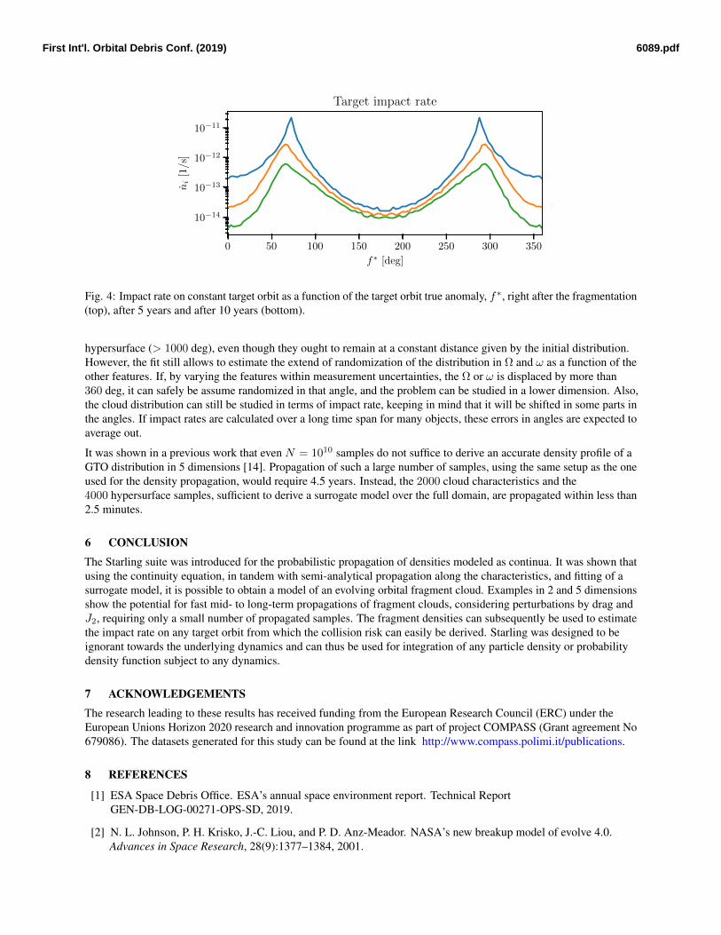
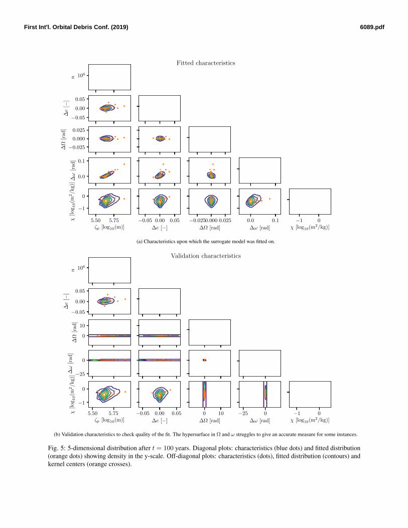
Fitting a GMM with 20 kernels to a 5-dimensional snapshot – i.e. requiring 420 parameters – takes about60-120 seconds and can be performed successfully up until t = 500 years, after which only 337 of the initially2000 cloud characteristics still remain. An example fit after 100 years of propagation, and 1153 remainingcharacteristics, is shown in 5a. As the secondary hypersurface follows the cloud samples (trailing or leading them onlyin Ω and ω), the resulting fit needs to be compared to a second set of verification cloud samples. Fig. 5b shows theverification samples, their respective densities and the estimated density from the surrogate model. It becomes evidentthat the ∆-space does not accurately represent the verification samples, because the secondary hypersurface does notinterpolate accurately enough across the full domain. Some of the samples are estimated to be far away from the


0 50 100 150 200 250 300 350

f∗ [deg]

10−14

10−13

10−12

10−11

ni

[1/s]

Target impact rate

Fig. 4: Impact rate on constant target orbit as a function of the target orbit true anomaly, f∗, right after the fragmentation(top), after 5 years and after 10 years (bottom).

hypersurface (> 1000 deg), even though they ought to remain at a constant distance given by the initial distribution.However, the fit still allows to estimate the extend of randomization of the distribution in Ω and ω as a function of theother features. If, by varying the features within measurement uncertainties, the Ω or ω is displaced by more than360 deg, it can safely be assume randomized in that angle, and the problem can be studied in a lower dimension. Also,the cloud distribution can still be studied in terms of impact rate, keeping in mind that it will be shifted in some parts inthe angles. If impact rates are calculated over a long time span for many objects, these errors in angles are expected toaverage out.

It was shown in a previous work that even N = 1010 samples do not suffice to derive an accurate density profile of aGTO distribution in 5 dimensions [14]. Propagation of such a large number of samples, using the same setup as the oneused for the density propagation, would require 4.5 years. Instead, the 2000 cloud characteristics and the4000 hypersurface samples, sufficient to derive a surrogate model over the full domain, are propagated within less than2.5 minutes.

6 CONCLUSION

The Starling suite was introduced for the probabilistic propagation of densities modeled as continua. It was shown thatusing the continuity equation, in tandem with semi-analytical propagation along the characteristics, and fitting of asurrogate model, it is possible to obtain a model of an evolving orbital fragment cloud. Examples in 2 and 5 dimensionsshow the potential for fast mid- to long-term propagations of fragment clouds, considering perturbations by drag andJ2, requiring only a small number of propagated samples. The fragment densities can subsequently be used to estimatethe impact rate on any target orbit from which the collision risk can easily be derived. Starling was designed to beignorant towards the underlying dynamics and can thus be used for integration of any particle density or probabilitydensity function subject to any dynamics.

7 ACKNOWLEDGEMENTS

The research leading to these results has received funding from the European Research Council (ERC) under theEuropean Unions Horizon 2020 research and innovation programme as part of project COMPASS (Grant agreement No679086). The datasets generated for this study can be found at the link http://www.compass.polimi.it/publications.

8 REFERENCES

[1] ESA Space Debris Office. ESA’s annual space environment report. Technical ReportGEN-DB-LOG-00271-OPS-SD, 2019.

[2] N. L. Johnson, P. H. Krisko, J.-C. Liou, and P. D. Anz-Meador. NASA’s new breakup model of evolve 4.0.Advances in Space Research, 28(9):1377–1384, 2001.


http://www.compass.polimi.it/publications

106n

−0.05

0.00

0.05

∆e

[−]

−0.025

0.000

0.025

∆Ω

[rad

]

0.0

0.1

∆ω

[rad

]

5.50 5.75ζp [log10(m)]

−1

0

χ[l

og10(m

2/k

g)]

−0.05 0.00 0.05

∆e [−]

−0.0250.000 0.025

∆Ω [rad]

0.0 0.1

∆ω [rad]

−1 0χ [log10(m2/kg)]

Fitted characteristics

(a) Characteristics upon which the surrogate model was fitted on.

106

n

−0.05

0.00

0.05

∆e

[−]

0

10

∆Ω

[rad

]

−25

0

∆ω

[rad

]

5.50 5.75ζp [log10(m)]

−1

0

χ[l

og10(m

2/k

g)]

−0.05 0.00 0.05

∆e [−]

0 10

∆Ω [rad]

−25 0

∆ω [rad]

−1 0χ [log10(m2/kg)]

Validation characteristics

(b) Validation characteristics to check quality of the fit. The hypersurface in Ω and ω struggles to give an accurate measure for some instances.

Fig. 5: 5-dimensional distribution after t = 100 years. Diagonal plots: characteristics (blue dots) and fitted distribution(orange dots) showing density in the y-scale. Off-diagonal plots: characteristics (dots), fitted distribution (contours) andkernel centers (orange crosses).


[3] J.-C. Liou, D. T. Hall, P. H. Krisko, and Opiela J. N. LEGEND - a three-dimensional LEO-to-GEO debrisevolutionary model. Advances in Space Research, (34):981–986, 2004.

[4] W. B. Heard. Dispersion of ensembles of non-interacting particles. Astrophysics and Space Science, 43:63–82,1976.

[5] C. R. McInnes. An analytical model for the catastrophic production of orbital debris. ESA Journal, 17:293–305,1991.

[6] F. Letizia, C. Colombo, and H. G. Lewis. Multidimensional extension of the continuity equation method fordebris clouds evolution. Advances in Space Research, 57:1624–1640, 2016.

[7] N. N. Gor’kavyi, L. M. Ozernoy, J. C. Mather, and T. Taidakova. Quasi-stationary states of dust flows underpoynting-robertson drag: new analytical and numerical solutions. The Astrophysical Journal, 488:268–276, 1997.

[8] A. Wittig, C. Colombo, and R Armellin. Long-term density evolution through semi-analyical and differentialalgebra techniques. Celestial Mechanics and Dynamical Astronomy, 128(4):435–452, 2017.

[9] S. Frey, C. Colombo, and S. Lemmens. Interpolation and integration of phase space density for estimation offragmentation cloud distribution. In Proceedings of the 29th AAS/AIAA Space Flight Mechanics Meeting, 2019.

[10] D. L. Talent. Analytic model for orbital debris environmental management. Journal of spacecraft and rockets,29(4):508–513, 1992.

[11] A. I. Nazarenko. The development of the statistical theory of a satellite ensemble motion and its application forspace debris modelling. In Proceedings of the 2nd European Conference on Space Debris, 1997.

[12] A. Rossi, L. Anselmo, A. Cordelli, P. Farinella, and C. Pardini. Modelling the evolution of the space debrispopulation. Planetary and Space Science, 46(11/12):1583–1596, 1998.

[13] F. Letizia. Extension of the density approach for debris cloud propagation. Journal of Guidance, Navigation, andControl, 41(12):2650–2656, 2018.

[14] S. Frey and C. Colombo. Transformation of satellite breakup distribution from cartesian coordinates to orbitalelements, submitted to the Journal of Guidance, Control, and Dynamics in November, 2019.

[15] T. T. Soong. Fundamentals of probability and statistics for engineers. John Wiley & Sons, Ltd., 2004.

[16] C. Colombo. Planetary orbital dynamics (PlanODyn) suite for long term propagation in perturbed environment.In Proceedings of the 6th International Conference on Astrodynamics Tools and Techniques (ICATT), 2016.

[17] S. Frey, C. Colombo, and S. Lemmens. Extension of the King-Hele orbit contraction method for accurate,semi-analytical propagation of non-circular orbits. Advances in Space Research, 64:1–17, 2019.

[18] S. Chib and E. Greenberg. Understanding the metropolis-hastings algorithm. The American Statistician,49(4):327–335, 1995.

[19] C. M. Bishop. Pattern Recognition and Machine Learning. Springer, 2006.

[20] A. Wittig, P. Di Lizia, R. Armellin, et al. Propagation of large uncertainty sets in orbital dynamics by automaticdomain splitting. Celestial Mechanics and Dynamical Astronomy, 122(3):239–261, 2015.

[21] D. McKnight and G. Lorenzen. Collision matrix for low earth orbit satellites. Journal of Spacecraft and Rockets,26(2):90–94, 1989.

[22] D. A. Vallado. Fundamentals of Astrodynamics and Applications. Hawthorne, CA: Microcosm Press, 4th edition,2013.

[23] A. Meurer, C. P. Smith, M. Paprocki, et al. Sympy: symbolic computing in python. PeerJ Computer Science, 3,2017.

[24] E. Jones, T. Oliphant, and P. Peterson. SciPy: Open source scientific tools for Python, http://www.scipy.org/,2001.


http://www.scipy.org/

Documents

Application of density-based propagation to fragment