Application of Convolution Theory for Solving Non-Linear Flow

Abstract In this paper we present the development of a rigorous ap-proach for the solution of non-linear partial differential equa-tions by use of the Laplace transformation — in particular, the convolution theorem for Laplace transforms. While the rigor of this new approach is general, our paper is devoted to the development, verification, and application of this method for the case of real gas flow in porous media. This paper focuses on verification of real gas flow solutions using the results of numerical simulation.

The major results of this work are:

Development of a general analytical approach in the Laplace domain for solving non-linear partial differen-tial equations. Verification and application of this new approach for the flow of a real gas in porous media.

We observe excellent agreement between the numerical and analytical results for the case of a single well produced at a constant rate in a closed reservoir. We conclude that this ap-proach could be adopted as a method of verification for nu-merical simulation, as well as for analytical modelling of the gas flow case — in particular, for modelling future perfor-mance directly and accurately, without numerical simulation or some weak approximation (p or p2 approximations, etc.).

In addition to the specific problem considered in this work, the flow of a real gas in porous media, we believe that it may be possible to extend this work for the development of analytical solutions for multiphase flow.

Introduction The primary objective of this work is to develop a closed form Laplace domain solution for the flow of a real gas from a well producing at a constant rate in a bounded circular reservoir. The need for this solution arises in the analysis of

gas well test data and gas well production data, where both analyses currently use approximate methods such as the pressure or pressure-squared methods, or rigorous, but tedious pseudovariables (pseudopressure and pseudotime). Our new solution can also be used for predicting reservoir performance as a high-speed simulation device — as opposed to using numerical reservoir simulation solutions.

While our new solution is not necessarily "easier" to apply than say the pseudovariables approach, our solution is essentially exact and it can be applied directly in performance prediction, as opposed to implicitly as in the case of the pseudotime approach (in theory, the pressure-dependent properties must be known). Our only "approximation" is the referencing of the time-dependent viscosity-compressibility product to the average reservoir pressure as a function of time, as computed from material balance. This referencing seems not only logical, but also appropriate (particularly when one considers that the pseudotime function also has this type of formulation).

We present the solution methodology where we recast the non-linear term of the right-hand-side of the gas diffusivity equation into a unique function of time. We do this without regard as to how to couple the time-pressure relationship, this will come later. We then use the convolution theorem for the Laplace transformation, as well as the definition of the Laplace transformation in order to "transform" our gas diffu-sivity equation into the Laplace domain.

In the Laplace domain, we recognize that the non-linear term is simply a transform function that can be incorporated directly into the "liquid equivalent" form of the Laplace do-main solution. The final issue is the resolution of how to sample the non-linear term, and as such, we empirically establish that for the constant rate case, the non-linear term should be sampled at the average reservoir pressure predicted from material balance. This sampling is later shown to yield an essentially exact comparison with the numerical solution and its pressure derivative functions.

We also present a comprehensive validation of our con-volution theory/Laplace transformation approach by com-paring our new solution to the results of a finite-difference reservoir simulation model for a variety of cases of gas reservoir size, initial pressure conditions, and gas properties. This chapter provides conclusive evidence that our new solu-tion yields an essentially exact solution for the bounded circular reservoir case.

SPE 84073

Application of Convolution Theory for Solving Non-Linear Flow Problems: Gas Flow Systems T.J. Mireles, BP, and T.A. Blasingame, Texas A&M U.

Copyright 2003, Society of Petroleum Engineers Inc. This paper was prepared for presentation at the SPE Annual Technical Conference and Exhi-bition held in Denver, Colorado, U.S.A., 5 – 8 October 2003. This paper was selected for presentation by an SPE Program Committee following review of information contained in an abstract submitted by the author(s). Contents of the paper, as presented, have not been reviewed by the Society of Petroleum Engineers and are subject to correction by the author(s). The material, as presented, does not necessarily reflect any posi-tion of the Society of Petroleum Engineers, its officers, or members. Papers presented at SPE meetings are subject to publication review by Editorial Committees of the Society of Petroleum Engineers. Electronic reproduction, distribution, or storage of any part of this paper for com-mercial purposes without the written consent of the Society of Petroleum Engineers is prohib-ited. Permission to reproduce in print is restricted to an abstract of not more than 300 words; illustrations may not be copied. The abstract must contain conspicuous acknowledgment of where and by whom the paper was presented. Write Librarian, SPE, P.O. Box 833836, Richardson, TX 75083-3836, U.S.A., fax 01-972-952-9435.

2 SPE 84073 __________________________________________________________________________________________________________________________________________________________________________________________________________________________________________________

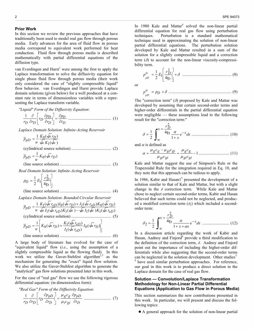
Prior Work In this section we review the previous approaches that have traditionally been used to model real gas flow through porous media. Early advances for the area of fluid flow in porous media correspond to equivalent work performed for heat conduction. Fluid flow through porous media is described mathematically with partial differential equations of the diffusion type.

van Everdingen and Hurst1 were among the first to apply the Laplace transformation to solve the diffusivity equation for single phase fluid flow through porous media (their work only considered the case of "slightly compressible liquid" flow behavior. van Everdingen and Hurst provide Laplace domain solutions (given below) for a well produced at a con-stant rate in terms of dimensionless variables with u repre-senting the Laplace transform variable.

"Liquid" Form of the Diffusivity Equation:

DD

DD

DDD t

prpr

rr ∂∂

=

∂∂

∂∂1 ......................................... (1)

Laplace Domain Solution: Infinite-Acting Reservoir

)()(1

1

0uKu

ruKu

p DpD =

(cylindrical source solution) ...................................... (2)

)(10 DpD ruK

up =

(line source solution) ................................................. (3)

Real Domain Solution: Infinite-Acting Reservoir

=

DD

D trEp42

1 21


Laplace Domain Solution: Bounded Circular Reservoir

)()()()()()()()(1

1111

0101

eDeD

DeDDeDpD ruKuIuuKruIu

ruKruIruIruKu

p−+

=

(cylindrical source solution) ...................................... (5)

+= )(

)()()(1

01

10 D

eD

eDDpD ruI

ruIruKruK

up


A large body of literature has evolved for the case of "equivalent liquid" flow (i.e., using the assumption of a slightly compressible liquid as the flowing fluid). In this work we utilize the Gaver-Stehfest algorithm2,3 as the mechanism for generating the "exact" liquid flow solution. We also utilize the Gaver-Stehfest algorithm to generate the "analytical" gas flow solutions presented later in this work.

For the case of "real gas" flow we use the following rigorous differential equation: (in dimensionless form):

"Real Gas" Form of the Diffusivity Equation:

D

pD

gii

gg

D

pDD

DD tp

cc

rp

rrr ∂

∂=

∂

∂

∂∂

µµ1 .......................... (7)

In 1980 Kale and Mattar4 solved the non-linear partial differential equation for real gas flow using perturbation techniques. Perturbation is a standard mathematical technique used in approximating the solution of non-linear partial differential equations. The perturbation solution developed by Kale and Mattar resulted in a sum of the solution for a slightly compressible liquid and a correction term (δ) to account for the non-linear viscosity-compressi-bility term.

δ+

=

DDt

rEppD 42

1 21

o ............................................... (8)

or δ+= Dpp

pDo ............................................................ (9)

The "correction term" (δ) proposed by Kale and Mattar was developed by assuming that certain second-order terms and higher-order differentials in the partial differential equation were negligible — these assumptions lead to the following result for the "correction term:"

dxex

trx

xDD

−+

=

∞= ∫ 1

421

2

αδ .................................... (10)

and α is defined as

1−=−

=gigi

gg

gigi

gigiggcc

ccc

µµ

µµµ

α ............................. (11)

Kale and Mattar suggest the use of Simpson's Rule or the Trapezoidal Rule for the integration required in Eq. 10, and they note that this approach can be tedious to apply.

In 1986, Kabir and Hasan15 presented the development of a solution similar to that of Kale and Mattar, but with a slight change in the δ correction term. While Kale and Mattar chose to neglect certain second-order terms, Kabir and Hasan believed that such terms could not be neglected, and produc-ed a modified correction term (δ2) which included a second-order term:

dxexx

trx

xDD

−++

=

∞= ∫ α

αδ1

421

2

2 .......................... (12)

In a discussion article regarding the work of Kabir and Hasan, Aadnoy and Finjord6 provide a third modification to the definition of the correction term, δ. Aadnoy and Finjord point out the importance of including the higher-order dif-ferentials while also suggesting that the second-order terms can be neglected in the solution development. Other studies7-

9 have used similar perturbation approaches. For reference, our goal in this work is to produce a direct solution in the Laplace domain for the case of real gas flow.

Solution — Convolution/Laplace Transformation Methodology for Non-Linear Partial Differential Equations (Application to Gas Flow in Porous Media)

This section summarizes the new contributions presented in this work. In particular, we will present and discuss the fol-lowing topics:

A general approach for the solution of non-linear partial

SPE 84073 3

differential equations. This solution incorporates the use of convolution theory and the Laplace transformation. A semi-analytical solution approach for the non-linear partial differential equation describing the flow of a real gas through porous media. This solution uses the techniques demonstrated in the general approach applied directly to the specific case of a gas well producing at a constant flowrate in a homogeneous, bounded circular reservoir. Two approaches for modeling the non-linear component in the behavior of a real gas. We include a discussion of both modeling approaches along with a sensitivity analysis which proves one method is much favorable for verifying the newly developed semi-analytical solution.

Laplace Transform/Convolution Approach for the Solution of General Non-Linear Partial Differential Equations

The development and details of the Laplace transform/con-volution approach are provided in Appendix A. We provide orientation and summary to these developments in this sec-tion.

Our starting point for this work is to state the non-linear partial differential equation (p.d.e.) for the flow of a real gas. This governing relation is given by:

D

pDD

D

pD

DD

pDt

pt

rp

rr

p∂

∂=

∂

∂+

∂

∂)(1

2

2β ...................... (13)

Where the non-linearity, β(tD), is given as:

gigi

ggD c

ct

µ

µβ =)( ..................................................... (14)

For convenience, we use the reciprocal of the non-linearity, β(tD), function — which is given as:

gg

gigi

DpDp c

ct

tRµ

µ

β==

)(1)( .................................. (15)

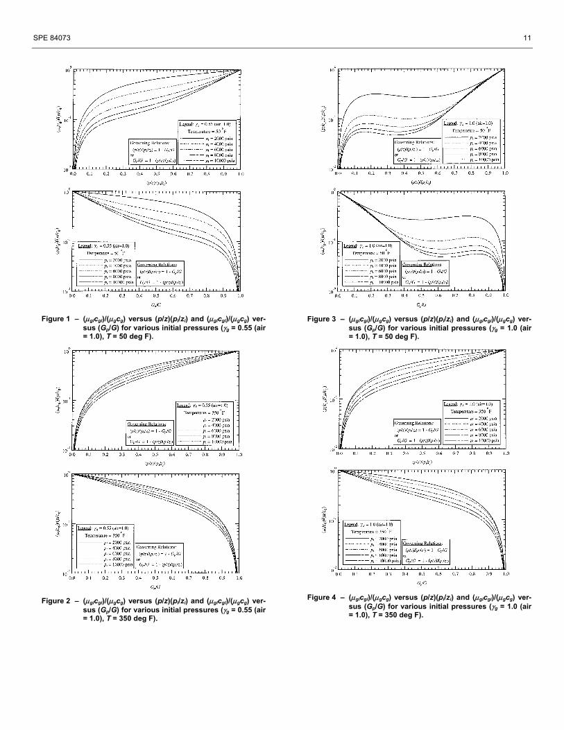
For orientation we present plots of )( Dp tR in Figs. 1-4 for various cases of gas gravity (γg), temperature (T), and initial reservoir pressure (pi). We note that the trends on these plots vary from "almost linear" to some function that appears to be a cubic (or higher) polynomial. This observation that )( Dp tR varies significantly has a profound effect on our work as we must accept that we cannot simply presume a functional form for )( Dp tR — but instead, it is likely that we will have to treat the )( Dp tR function as a data function (i.e., a function defined by the data — e.g., we could use linear segments to represent the data). This issue will be addressed in a later section.

Given the general non-linearity function, β(tD), (or the recipro-cal function, )( Dp tR ), we recognize that this term cannot be ignored (at least in a general sense). Writing a generalized form of Eq. 13 (i.e., a non-linear partial differential equation) gives us:

tyty

∂∂

=∇ )(2 β ........................................................ (16)

We immediately recognize that β(t) ∂y/∂t is of the form:

)()()( 21 tftftyt =

∂∂β ............................................... (17)

From ref. 10, the Laplace transform of the f1(t)f2(t) product is:

{ } dzzufzfic

icitftfL )()(

21)()( 2121 −

∞+

∞−= ∫π

......... (18)

Eq. 18 is not a particularly useful formulation/identity. How-ever, we can write the f1(t)f2(t) product as a convolution-type formulation. This gives:

τττ dtgft

tftf )()(0

)()( 121 −= ∫ .............................. (19)

Taking the Laplace transform of Eq. 19 yields:

{ }

−= ∫ τττ dtgft

LtftfL )()(0

)()( 121

or { } )()()()( 121 uguftftfL = ....................................... (20)

Where g(u) = L{g(t)}, and g(t) is then defined by the convolu-tion identity.

Substituting f1(t) = ∂y/∂t and f2(t) = β(t) into Eq. 20 yields

τττ

β dtgyt

tyt )(

0)( −

∂∂

=∂∂ ∫ ..................................... (21)

Substituting Eq. 21 into Eq. 17 gives us our "convolution" form of the non-linear partial differential equation:

τττ

dtgyty )(

02 −

∂∂

=∇ ∫ .......................................... (22)

Our strategy is to use Eq. 21 to estimate the g(t) function. We recognize that Eq. 21 does not offer much insight into the estimation of g(t) (obviously, g(t) is problem-dependent). We will address the issue of g(t) as the next discussion topic. The relevant issue is that we can take the Laplace transform of Eq. 22, which is given as:

)( 0)]()([)(2 ugtyuyuuy =−=∇ ............................. (23) Depending on the initial condition (recall that our use of dimensionless pressure yields 0 (zero) for the t=0 condition), which reduces Eq. 23 to:

)()()(2 uyuuguy =∇ ............................................... (24) The form of Eq. 24 should be familiar to practitioners of reser-voir engineering, as Eq. 24 is of the same form as the Laplace domain solution for the case of dual porosity/naturally-frac-tured reservoirs. As such, we can simply substitute the ug(u) product into each of the "u" terms in the appropriate Laplace domain solutions for liquid flow (i.e., Eqs. 2, 3, 5, and 6). However, we must recognize the exception of the 1/u term in front of each relation — do not substitute the ug(u) product into the leading 1/u term .

For example, in our present work we focus on the case of a bounded circular reservoir — using the ug(u) substitution in the "cylindrical source" solution (i.e., Eq. 5) gives us:

))(())(()())(())(()())(())(())(())((1

1111

0101

eDeD

DeDDeD

pD

ruugKuugIuuguugKruugIuugruugKruugIruugIruugK

u

p

−

+

=

.................................................................................. (25) Eq. 25 becomes our base relation for validation as an "analy-tical" real gas flow solution. Eq. 25 will be used as the basis

4 SPE 84073 __________________________________________________________________________________________________________________________________________________________________________________________________________________________________________________

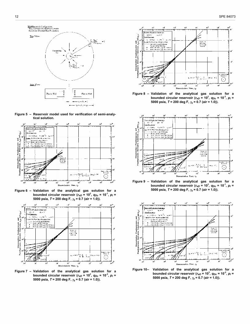
for comparison/validation with numerical simulation — this effort is discussed in detail in a later section. For reference, the configuration of the well/reservoir is given in Fig. 5.

We are now at a point where we need to define g(t) (and, of course, g(u)). From Appendix A, we have the following identity: (see Appendix A for details)

)(11)(

uRuug

p= ....................................................... (26)

We recall that )( Dp tR is defined as:

gg

gigi

DpDp c

ct

tRµ

µ

β==

)(1)( .................................. (15)

The next challenge is to take )( Dp tR data into the Laplace domain — this effort is not overly tedious, but we must realize that the integrity of the data must be maintained. In consi-dering Figs. 1-4, we recognize that the )( Dp tR function varies significantly — simply assigning a regression model to the

)( Dp tR data may not be optimal, nor wise. As such, we have chosen to take the entire )( Dp tR function into the Laplace domain using the method of Roumboutsos and Stewart.11

For a given table of data (i.e., f(t) versus t) the Roumboutsos and Stewart algorithm is implemented using:

+

−+

−

=

−

−

−

−−−

=

−

∑1

1

1

)(

)1(

1)(

1

2

1

2

n

ii

utn

ututi

n

i

ut

em

eem

em

uuf ..................... (27)

Where the slope terms (i.e., the mi - values) are taken as back-ward differences given by:

)-()-(

11

−

−=iiii

i ttff

m ........................................................ (28)

In Appendix A we provide additional discussion regarding the Roumboutsos and Stewart algorithm, as well as the potential use of regression models for the )( Dp tR data function. We strongly recommend use of the Roumboutsos and Stewart algorithm for general applications — it is both easy to imple-ment and robust.

Validation As a mechanism for validation, we compare results from numerical simulation and our proposed solution for the case of a volumetric dry gas reservoir produced at a constant produc-tion rate. Our results are generated using Eqs. 25 and 26, along with the Roumboutsos and Stewart algorithm (Eqs. 27 and 28), which is used to compute the )(uRp function).

The primary validation cases (Figs. 6-15) were generated us-ing the data given below:

Reservoir Properties: Wellbore radius, rw = 0.25 ft Net pay thickness, h = 30 ft Formation permeability, k = 1.0 md Porosity, φ (fraction) = 0.30 Initial reservoir pressure, pi = 5000 psia

Fluid Properties: Gas specific gravity, γg = 0.7 (air = 1.0) Reservoir temperature, T = 200 deg F

Validation Plots: (pi=5000 psia, γg=0.7, T=200 deg F)

Plotting Functions (all cases) — ppD and ppD' vs. tD

reD qDc Fig. 1x102 1x10-1 6 1x102 1x10-2 7 1x102 1x10-3 8 1x103 1x10-1 9 1x103 1x10-2 10 1x103 1x10-3 11 1x104 1x10-1 12 1x104 1x10-2 13 1x104 1x10-3 14

In order to assess the influence of rate on the new gas flow solution (i.e., the classic test of a non-linear partial differential equation), we established a "dimensionless constant rate" vari-able, qDc, which is defined as:

−

−=

43)ln(

)(2141 eD

abn,ppi

ggigiDc r

ppq

khB

.qµ

. (29)

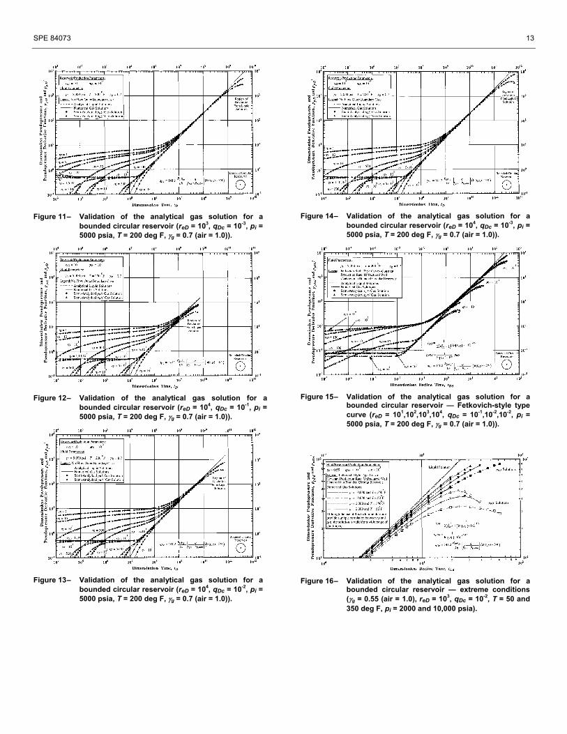
In reviewing Figs. 6-14 we note that the analytical and nu-merical gas flow solutions compare well — extremely well for all cases considered in this suite of figures. It is worth noting that in Figs. 6-14 we have compared solutions at the wellbore and in the reservoir — and all comparisons are in excellent agreement, suggesting that the proposed analytical gas flow solution is a universal solution.

In Fig. 15 we present a "composite" plot of cases for reD= 1x101, 102, 103, and 104 — these are essentially the same cases considered in Figs. 6-14, except that only the cases for rD=1 (i.e., the wellbore pressure solutions) are compared on Fig. 15.

We note that we have modified the definitions of the dimen-sionless time and pressure plotting functions in order to develop the "composite" plot (i.e., Fig. 15). The plotting func-tions used for Fig. 15 are defined as:

DeDeD

D trr

t

−−

=

21)ln(

1)1( 2

12 ............................ (30)

pDeD

pDd pr

p

−

=

21)ln(

1 ...................................... (31)

pr

p 'pD

eD

'pDd

−

=

21)ln(

1 ..................................... (32)

From our observations of the performance shown on Fig. 15 we can conclude that the analytical and numerical gas flow solutions are in excellent agreement. We can further comment that this "composite" plot permits us to compare the effects of the qDc variable on all cases — and we can comment that the new solution does reproduce the same features as the numeri-

SPE 84073 5

cal solutions for times when the qDc variable affects the performance (generally late times). Overall, we can conclude from Fig. 15 that the proposed analytical gas flow solution is consistent and reproducible.

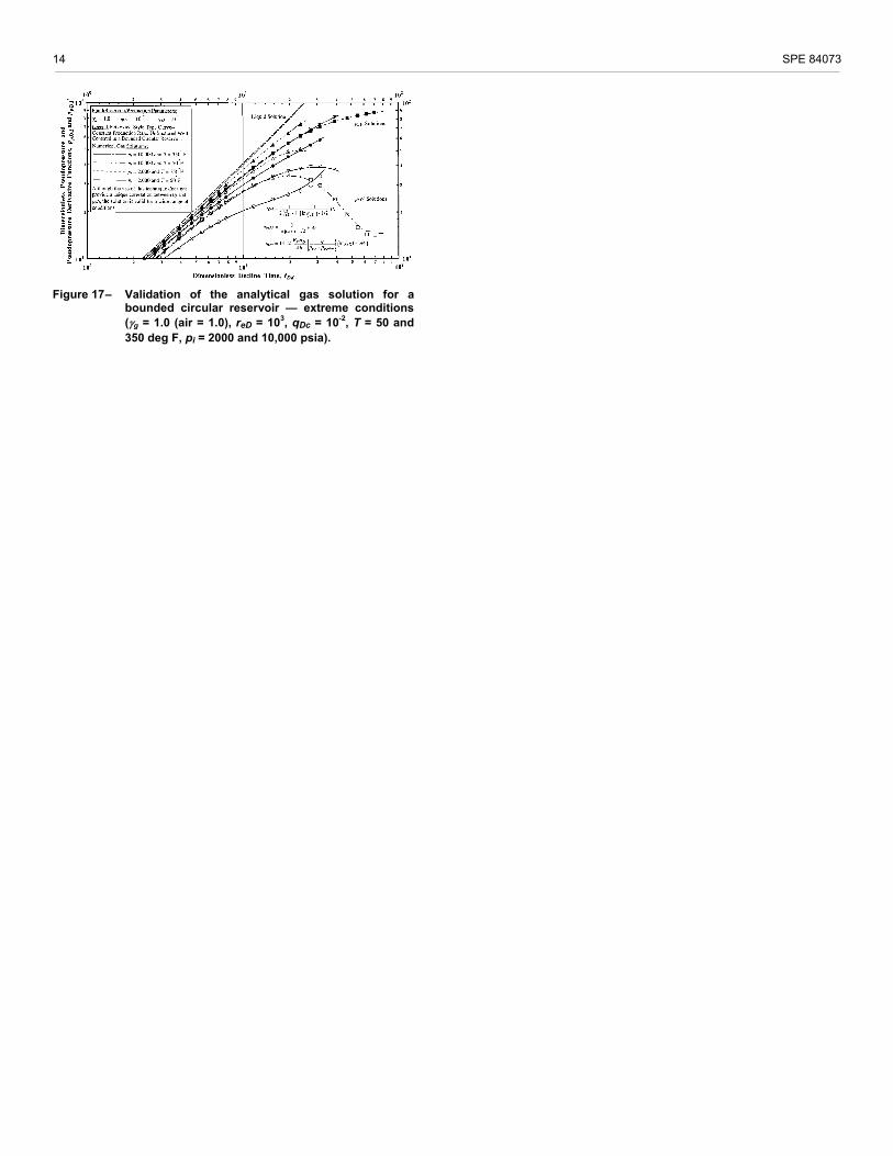
The final issue that we might wish to consider is that of "extreme" cases of fluid type, temperature, and initial reservoir pressure. Fig. 16 (γg=0.55 (methane)) and Fig. 17 (γg=1.0 (rich gas)) illustrate the "composite" behavior of a variety of "extreme" cases — and we note that the new analytical gas flow solution compares well to numerical solution for all cases considered. We note that Figs. 16 and 17 use the same plot-ting functions as Fig. 15 (i.e., Eqs. 30, 31, and 32) Summary and Conclusions

Summary We have developed and successfully validated a new semi-analytical solution approach for the gas diffusivity equation. In particular, our solution represents the case of a gas well producing at a constant flowrate in a homogeneous, bounded circular reservoir. Our approach is rigorous in its formula-tion of the viscosity-compressibility product (i.e., the non-linear term in the gas diffusivity equation). We developed our solution approach using convolution theory and the defi-nition of the Laplace transformation.

We considered the viscosity-compressibility product to be only time-dependent, and we used this relationship to develop a transform function for the viscosity-compressi-bility product in the Laplace domain. The new solution is evaluated using the "liquid" flow solution (i.e., the linear solution), coupled with our transform function which represents the behavior of the viscosity-compressibility pro-duct. The resulting solution has exactly the same form (but obviously not the same function) as the case of a well in a naturally fractured reservoir.

We have successfully verified our new semi-analytical solution by comparison with numerical results from a finite-difference reservoir simulator for dry gas flow. Our sensi-tivity study considered a variety of reservoir sizes, production rates, and ranges of gas properties. We note excellent com-parisons of computed pressures and pressure derivative functions for all cases — which we believe uniquely verifies our approach as well as its application to engineering pro-blems.

Conclusions We consider the following to be the most important concepts and conclusions developed in this work:

1. Based on comparisons with results from numerical simulations, we have proven that we can apply con-volution theory and the Laplace transformation as a means to solve the non-linear gas diffusivity equation which describes gas flow in porous media. We used this approach to solve the particular case of a gas well produced at a constant flowrate in a bounded (no flow) circular reservoir.

2. We observe that the behavior of the numerical and semi-analytical solutions for pseudopressure and time are not completely unique in that the behavior during

depletion (i.e., pseudosteady-state) depends on flow-rate, initial pressure, and the pressure and temperature variations in gas properties. Such dependence is the trademark of a non-linear problem.

3. We found that the time-dependence of the viscosity-compressibility term can be accurately represented by a tabulated data function as well as using a functional form to model the behavior of the data. We noted the following:

The Roumboutsos and Stewart algorithm for trans-forming a data table into the Laplace domain is simple to implement, is highly reliable, and is very accurate, and

Of the functional models we tested, the general polynomial form gave the best results, although the exponential data model did match the viscosity-compressibility data quite well. A comparison of our simulated results showed that both the polyno-mial and exponential models give satisfactory re-sults. However, we chose to use the Roumboutsos and Stewart approach in order not to bias our results to a particular data model.

Recommendations for Future Work Future work must explore the case of constant wellbore pressure production, as well as the case of general variable-rate convolution. In addition, other reservoir/well models must be verified. For example, gas flow in vertically-fractured wells, horizontal wells, and naturally fractured reservoirs are of significant interest to the petroleum industry and should be thoroughly investigated.

Finally, future work should also focus on the development of closed-form solutions in the real time domain — i.e., explicit inversion of the Laplace domain solutions we have presented in this work. Nomenclature

Field Variables (Pressure, Formation, and Fluid Properties)

an = Coefficients for exponential/polynomial models Bg = Gas formation volume factor, RB/MSCF Bgi = Gas formation volume factor at pi, RB/MSCF cg = Gas compressibility, psia-1 cgi = Gas compressibility at pi, psia-1 gc = Gas compressibility at ,p psia-1 ct = Total system compressibility, psia-1 cti = Total system compressibility at pi, psia-1 g(u) = Laplace transform function of the non-linearity G = Original gas-in-place, MSCF Gp = Cumulative gas production, MSCF h = Formation thickness, ft k = Formation permeability, md p = Pressure, psia p = Average reservoir pressure, psia pD = Dimensionless pressure response )(upD = Laplace transform of dimensionless pressure pi = Initial reservoir pressure, psia pp = Normalized pseudopressure, psia

6 SPE 84073 __________________________________________________________________________________________________________________________________________________________________________________________________________________________________________________

pp,abn = Normalized pp at abandonment pressure, psia ppD = Dimensionless normalized pseudopressure ppD' = Logarithmic derivative of ppD ppDd = Dimensionless normalized pseudopressure func-

tion (Eq. 31) ppDd' = Logarithmic derivative of ppDd (Eq. 32) p

pDo = Dimensionless pseudopressure solution for per-

turbation solutions (Eq. 8) ppi = Normalized pseudopressure at pi, q = Gas flow rate, MSCF/D qDc = Dimensionless gas flowrate (constant) u = Laplace transform variable, dimensionless r = Radius, ft rD = Dimensionless radius reD = Dimensionless drainage radius

)( Dp tR = Inverse of the non-linear viscosity-compressibility function evaluated at average reservoir pressure, dimensionless (time domain)

)(uRp = Laplace transform of the inverse of the non-linear viscosity-compressibility function evaluated at average reservoir pressure, dimensionless

rw = Wellbore radius, ft rw' = Effective wellbore radius, ft t = Time, days tD = Dimensionless time (based on cti) tDd = Dimensionless "decline" time (Eq. 30) T = Temperature, Deg F x = Boltzman transform, dimensionless y = Dummy pressure-type of variable z = Real gas deviation factor, dimensionless z = Real gas deviation factor at ,p dimensionless zi = Real gas deviation factor at pi, dimensionless

Greek Letter Variables α = Non-linear µgcg function (defined by Kale and

Mattar), dimensionless )( Dtβ = Non-linear µgcg function, dimensionless

)( Dp tβ = Non-linear µgcg function at ,p dimensionless δ = Correction term to account for the non-linearity in

gas flow systems (Kale and Mattar), dimension-less

δ2 = Correction term to account for the non-linearity in gas flow systems (Kabir and Hasan), dimension-less

φ = Porosity, fraction γg = Gas specific gravity (air=1.0) µg = Gas viscosity, cp gµ = Gas viscosity at ,p cp µgi = Gas viscosity at pi, cp τ = Dummy time-type variable, days

Subscripts: p = Variable evaluated at p D = Dimensionless variable

Special Functions/Operators: E1 = Exponential integral I0(x) = Modified Bessel function (1st kind, zero order) I1(x) = Modified Bessel function (1st kind, 1st order) K0(x) = Modified Bessel function (2nd kind, zero order)

K1(x) = Modified Bessel function (2nd kind, 1st order) L = Laplace domain operator (from real domain to

Laplace domain)

References

1. van Everdingen, A.F. and Hurst, W.: "The Application of the Laplace Transformation to Flow Problems in Reservoirs," Trans. AIME (Dec. 1949) 305-324B.

2. Kale, D. and Mattar, L.: "Solution of a Non-Linear Gas Flow Equation by the Perturbation Technique," JCPT (Oct.-Dec. 1980) 63-67.

3. Gaver, D.P., Jr.: "Observing Stochastic Processes and Approximate Transform Inversion," Operations Re-search, vol. 14, No. 3 (1966), 444-459.

4. Stehfest, H.: "Numerical Inversion of Laplace Transforms," Communication of the ACM (Jan. 1970) 13, No. 1, 47-49. (Algorithm 368 with correction (October 1970),13, No. 10).

5. Kabir, C.S. and Hasan, A.R.: "Prefracture Testing in Tight Gas Reservoirs," SPEFE (April 1986) 128-138.

6. Aadnoy, B.S. and Finjord, J.: "Discussion of Prefracture Testing in Tight Gas Reservoirs," SPEFE (April 1986), 628-629.

7. Finjord, J.: "An Analytical Study of Pseudo-time for Pressure Drawdown in a Gas Reservoir," paper SPE 15205 (1985, unsolicited) Available from SPE Richard-son, Texas.

8. Kikani, J. and Pedrosa, O.A., Jr.: "Perturbation Analysis of Stress-Sensitive Reservoirs," SPEFE (Sept. 1991), 379-386.

9. Wang, Y.: "Discussion of Perturbation Analysis of Stress-Sensitive Reservoirs," SPEFE (Sept. 1992), 268.

10. Roberts, G.E., and Kaufman, H.: Table of Laplace Transforms, W.B. Saunders Company, Philadelphia, 1964.

11. Roumboutsos, A. and Stewart, G.: "A Direct Decon-volution or Convolution Algorithm for Well Test Analy-sis," paper SPE 18157 presented at the 1988 SPE Annual Technical Conference and Exhibition, Houston, TX, 2-5 Oct. 1988.

Appendix A — Derivation of An Exact Laplace Trans-form Formulation for The Real Gas Diffusivity Equa-tion Using a Convolution Approach for The Non-Linear Viscosity-Compressibility Product

Development of the Convolution Formulation for a Non-Linear Partial Differential Equation The general form of a non-linear partial differential equation is given by

tyty

∂∂

=∇ )(2 β ....................................................... (A.1)

The key to our convolution technique is to recognize that the left-hand-side (LHS) of Eq. A.1 can be transformed — but the right-hand-side (RHS) is not in a form that can be readily transformed. Specifically, we recognize that the β(t) ∂y/∂t term is of the form

)()()( 21 tftftyt =

∂∂β .............................................. (A.2)

From Roberts and Kaufman (ref. 10, Section 1-Operations, p.

SPE 84073 7

4, Eq. 16), the Laplace transform of the f1(t)f2(t) product is:

{ } dzzufzfic

icitftfL )()(

21)()( 2121 −

∞+

∞−= ∫π

....... (A.3)

Where u is the Laplace transform parameter, and the functions )(1 uf and )(2 uf are the Laplace transforms of the functions

f1(t) and f2(t), respectively. We note that Eq. A.3 is not a useful form, but from this form we can suggest a different approach — writing the f1(t)f2(t) product as a convolution-type formulation. This concept leads to

τττ dtgft

tftf )()(0

)()( 121 −= ∫ ............................ (A.4)

Taking the Laplace transform of Eq. A.4 gives us:

{ }

−= ∫ τττ dtgft

LtftfL )()(0

)()( 121

or { } )()()()( 121 uguftftfL = ..................................... (A.5)

Where g(u) = L{g(t)}, and g(t) is then defined by the convolu-tion identity. Letting f1(t) = ∂y/∂t and f2(t) = β(t), then, upon substitution into Eq. A.4 we obtain the following identity:

τττ

β dtgyt

tyt )(

0)( −

∂∂

=∂∂ ∫ ................................. (A.6a)

Or in terms of a "dimensionless" time function (tD=t/tch), we have:

τττ

β dtgyt

tyt D

D

DD )(

0)( −

∂∂

=∂∂ ∫ ...................... (A.6b)

substituting Eq. A.6a into Eq. A.1 gives us:

τττ

dtgyty )(

02 −

∂∂

=∇ ∫ ........................................ (A.7)

Of course, the trick is to determine the g(t) function from the identity given by Eq. A.6a (or A.6b), but this issue is pro-blem-specific — and must be addressed as such. However, the relevant issue is that we can take the Laplace transform of Eq. A.7. Taking the Laplace transform of Eq. A.7 we have

)( 0)]()([)(2 ugtyuyuuy =−=∇ ........................... (A.8) We note that the form given by Eq. A.8 should be useful for second order, diffusion-type partial differential equations.

Application of the Convolution/Laplace Transform Ap-proach to the Real Gas Diffusivity Equation The dimensionless form of the real gas diffusivity equation is given as

D

pD

tigi

tg

D

pDD

DD tp

cc

rp

rrr ∂

∂=

∂

∂

∂∂

µµ1

or

D

pD

tigi

tg

D

pD

DD

pDt

pcc

rp

rr

p∂

∂=

∂

∂+

∂

∂

µµ1

2

2 ..................... (A.9)

where µg and ct are assumed to be functions of both dimen-sionless pseudopressure and dimensionless time. By com-parison with Eq. A.1, we define the β(tD) function as

tigi

tgD c

ct

µµ

β =)( .................................................... (A.10)

Substituting Eq. A.10 into Eq. A.9, we obtain

D

pDD

D

pD

DD

pDt

pt

rp

rr

p∂

∂=

∂

∂+

∂

∂)(1

2

2β ................... (A.11)

Expressing the right-hand-side of Eq. A.11 in the convolution form (e.g., Eq. A.6b) gives us

τττ

β dtgpt

tp

t DpDD

D

pDD )(

0)( −

∂

∂=

∂

∂

∫ .............. (A.12)

Substituting Eq. A.12 into Eq. A.11 yields

τττ

dtgpt

rp

rr

pD

pDD

D

pD

DD

pD )(0

12

2−

∂

∂=

∂

∂+

∂

∂

∫ .. (A.13)

Taking the Laplace transform of Eq. A.13

)( 0)]()([12

2ugtpupu

drpd

rdr

pdDpDpD

D

pD

DD

pD =−=+

.............................................................................. (A.14) where, after applying the initial condition (ppD(rD,tD=0)=0), Eq. A.14 reduces to:

)()(12

2upuug

drpd

rdr

pdpD

D

pD

DD

pD =+ ................... (A.15)

Eq. A.15 has exactly the same form (but obviously not the same function) as the generalized formulation for dual poro-sity or naturally fractured reservoirs. But what is the g(u) function?

Eq. A.12 defines the g(tD) function — but how do we evaluate this function? We require both β(tD) and ∂ppD/∂tD neither of which are known a priori — but perhaps we can approximate these functions, or use the known behavior of a function for a particular flow regime. (e.g., pseudosteady-state). This issue is addressed in the next section.

Modelling the Non-Linear Term In this section we consider how to determine the g(tD) func-tion. Although not obvious, we can establish a relationship for ∂ppD/∂tD using the volumetric dry gas material balance equa-tion which uses the average reservoir pressure to correlate reservoir behavior. While this may seem limiting, our approach is actually quite sound, and will be verified by comparison to performance data generated using numerical simulation of a volumetric gas reservoir.

Writing the time derivative term and its chain rule expansion, we have

D

p

p

pD

D

pDtt

tzp

zpp

pp

pp

tp

∂∂

∂∂

∂∂

∂

∂

∂

∂=

∂

∂ )/()/(

.............. (A.16)

In order to reconcile the terms in Eq. A.16 we will use the following identities (as well as other definitions (e.g., cg)):

Dimensionless Pressure:

)( ppigigig

DcpD ppBq

khpp −=µ

....................... (A.17)

Normalized Pseudopressure:

8 SPE 84073 __________________________________________________________________________________________________________________________________________________________________________________________________________________________________________________

dpz

pp

pp

zp

gbasei

igip

µ

µ∫= ................................ (A.18)

Dimensionless Time: (assume cgi ≈ cti)

trc

kttwgigi

DcD 2φµ= ......................................... (A.19)

Where the tDc and pDc constants are given by:

Constant

Darcy Units

Field Units

SI Units

tDc 1 6.33x10-3 3.557x10-6 pDc 2π 7.081x10-3 or 1/141.2 5.356x10-4

The gas material balance equation is given by

−=

GG

zp

zp p

ii 1 ................................................... (A.20)

Assuming a constant gas flow rate, qg, we have Gp=qg t, which, when substituted into Eq. A.20 gives us:

−=

Gtq

zp

zp g

ii 1 ................................................... (A.21)

Differentiating Eq. A-17 with respect to pressure, we obtain:

gigigDc

pDBq

khpp

pµ

−=∂

∂................................... (A.22)

Taking the derivative of pseudopressure (Eq. A.18) with re-spect to pressure, we have:

zp

pz

pp

gi

igipµ

µ=

∂

∂................................................. (A.23)

The ∂(p/z)/∂p term is expanded to yield:

∂∂

−=∂∂

−=∂

∂−=

∂∂

pz

zpzp

pz

z

pzp

zpzp

zp 111)/1(1)/(2

Where the gas compressibility, cg, is defined as:

pz

zpcg ∂

∂−=

11 ....................................................... (A.24)

Substituting Eq. A.24 into the previous relation gives us:

gczp

pzp

=∂

∂ )/( ....................................................... (A.25)

The reciprocal of Eq. A.25 is given by

gcpz

zpp 1

)/(=

∂∂ ...................................................... (A.26)

Taking the derivative of the gas material balance equation (Eq. A.21) with respect to time

gii q

Gzp

tzp 1)/(

−=∂

∂ ............................................... (A.27)

Taking the time derivative of Eq. A.19 gives

2wgigi

DcD

rc

ktt

t

φµ=

∂∂ ......................................... (A.28)

The reciprocal of Eq. A.28 is

k

rc

ttt wgigi

DcD

21 φµ

=∂∂ ........................................ (A.29)

Substituting Eqs. A.22, A.23, A.26, A.27 and, A.29 into Eq.

A.16 we obtain:

−

−=

∂

∂

krc

t

qGz

p

cpz

zp

pz

Bqkhp

tp

wgigi

Dc

gii

g

gi

igi

gigigDc

D

pD

21

1

1

φµ

µ

µ

µ

x

x

x

x

And, Rearranging and canceling like terms gives:

gg

gigi

giw

DcDc

D

pDcc

GBhr

tp

tp

µ

µφ 2=

∂

∂

The above relation is taken implicitly as a function of average reservoir pressure (recall that we used the gas material balance equation for a volumetric dry gas reservoir). There-fore, the relation given above is referenced to the average reservoir pressure as follows:

gg

gigi

giw

DcDc

D

avg,Dpcc

GBhr

tp

tp

µ

µφ 2=

∂

∂

We also assume that ct=cg, which is should be valid for most applications in the case of a volumetric dry gas reservoir. Therefore, our final result is given by:

gg

gigi

giw

DcDc

D

avg,Dpcc

GBhr

tp

tp

µ

µφ 2=

∂

∂........................ (A.30)

Substituting Eq. A.30 into Eq. A.12 gives

ττµ

µφ

µ

µφβ

dtgcc

GBhr

tpt

cc

GBhr

tp

t

Dgg

gigi

giw

DcDcD

gg

gigi

giw

DcDc

D

)(0

)(

2

2

−

=

∫

Canceling like terms gives

ττµ

µ

µ

µβ dtg

cct

cc

t Dgg

gigiD

gg

gigiD )(

0)( −= ∫ ......... (A.31)

Recalling the definition of β(tD) (Eq. A.10), we have:

gigi

ggD c

ct

µ

µβ =)( .................................................. (A.10)

Assuming, as we have for previous results, that the µgcg pro-duct is evaluated at the average pressure, Eq. A.10 becomes

gigi

ggDp c

ct

µ

µβ =)( ............................................... (A.32)

Substituting Eqs. A.10 and A.32 into Eq. A.31 we obtain

1)()()(

)(1

0≈=−∫ Dp

DD

p

D

ttdtg

t

ββ

τττβ

............... (A.33)

SPE 84073 9

Taking the Laplace Transform of Eq. A.33 gives us:

)()(

11 ugt

Lu Dp

=β

Or, solving for g(u), we have:

=

)(1

11)(

Dp tL

uug

β

.......................................... (A.34)

Defining a reciprocal function, ),( Dp tR we obtain:

gg

gigi

DpDp c

ct

tRµ

µ

β==

)(1)( ............................... (A.35)

Substituting Eq. A.35 into Eq. A.34 gives us:

)(11)(

uRuug

p= .................................................... (A.36)

Where: )}({)( Dpp tRLuR =

Using the )( Dp tR definition (Eq. A.35), Eq. A.33 becomes

τττ dtgRt

DpD

)()(0

1 −= ∫ ................................... (A.37)

Application Approach

Recalling the general Laplace transform result based on the convolution approach (i.e., Eq. A.15), we have:

)()(12

2upuug

drpd

rdr

pdpD

D

pD

DD

pD =+ ................... (A.15)

Where Eq. A.15 also has the following "compact" form:

)()(1 upuugdrpd

rdr

dr pD

D

pDD

DD=

Where, as in the case of a naturally fractured reservoir, the ug(u) function is substituted for all u terms in the Laplace do-main (except for the 1/u term given in front of a given solu-tion).

Specifically, Eq. A.15 implies that )]([ )()( uugpugup Dgas,Dp = ............................... (A.38)

where )(upD is the "liquid equivalent" (or linear p.d.e.) solu-tion. We obtain the g(u) function from the identity:

)(11)(

uRuug

p= .................................................... (A.36)

We must therefore develop strategies to obtain the )( Dp tR function. Recall that )( Dp tR is given by Eq. A.35:

gg

gigiDp c

ctR

µ

µ=)( ................................................ (A.35)

Recalling the gas material balance equation for volumetric gas reservoir produced at a constant bottomhole pressure (Eq. A.21), we have:

−=

Gtq

zp

zp g

ii 1 ................................................... (A.21)

Substituting Eq. A.19 into Eq. A.21 gives

−= D

wgigi

Dc

g

ii t

krc

tGq

zp

zp

211

φµ................... (A.39)

Using Eqs. A.35 and A.39, and a table of gas properties (µg, ct, and z), we perform a table look-up of the non-linearity function, ))/(()( gggigiDp cctR µµ= based on zp/ — the table given below provides a schematic format for computing the )( Dp tR function.

t

(data)

tD (Eq. A.19)

zp/ (Eq. A.21

or Eq. A.39)

gg

giiDp c

ctR

µ

µ=)(

(Eq. A.35) xxx xxx xxx

xxx xxx xxx

xxx xxx xxx

xxx xxx xxx

This approach should be used as a table look-up — e.g., specify t or tD, and return with ).( Dp tR Using this approach requires an algorithm or function to transform the )( Dp tR data into the Laplace domain. This issue is discussed in the next section.

Roumboutsos and Stewart Algorithm for )( Dp tR

The most consistent approach for modelling the )( Dp tR function in the Laplace domain is to actually bring the data table ( )( Dp tR versus tD) into the Laplace domain. In this work we chose to use the Roumboutsos and Stewart algorithm as it is simple, straightforward to program, and generally very accurate. The Roumboutsos and Stewart algorithm11 considers the data to be connected by piecewise linear functions (i.e., individual data points are connected using linear segments).

For a given table of data (i.e., f(t) versus t) the Roumboutsos and Stewart algorithm is given as

+

−+

−

=

−

−

−

−−−

=

−

∑1

1

1

)(

)1(

1)(

1

2

1

2

n

ii

utn

ututi

n

i

ut

em

eem

em

uuf .................. (A.40)

where the slope terms (i.e., the mi - values) are taken as back-ward differences given by:

)-()-(

11

−

−=iiii

i ttff

m ..................................................... (A.41)

Curve Fit Approach for )( Dp tR

Alternatively, we could curve fit )( Dp tR using a model in terms of tD. We are reluctant to recommend this as a general application due to the possible variations in gas properties that could yield an )( Dp tR trend that is not well fitted by a specific model. Such an event would yield poor results and possibly bias the application in general. We believe that the best approach is to take the )( Dp tR data directly into the Laplace domain using an algorithm such as the Roumboutsos and Stewart method.

10 SPE 84073 __________________________________________________________________________________________________________________________________________________________________________________________________________________________________________________

Still, the application of data models for the )( Dp tR is worth-while, especially for the possible development of closed form real domain solutions — although this concept is not investi-gated in this work. Experience and intuition show that a sin-gle-term exponential function, as well as cubic and higher polynomial functions are well-suited to match the behavior of the )( Dp tR function. These functions are shown below.

The polynomial form of the )( Dp tR -tD trend is given as

nDnDDD

gg

gigiDp

ta...tatata

cc

tR

+++++=

=

33

2211

)(µ

µ

....... (A.42)

Taking the Laplace transform of Eq. 41 gives

143

32

21 !3!2!1

)(

++++++=

=

nn

gg

gigip

u

an...

u

a

u

a

u

au

cc

LuRµ

µ

...... (A.43)

Recalling the g(u) identity, Eq. A.36, we have

)(11)(

uRuug

p= .................................................... (A.36)

Substituting Eq. A.43 into Eq. A.36, we obtain

nn

p

u

an...u

a

u

aua

uRuug

!3!2!1

1

)(11)(

33

221 +++++

=

=

........... (A.44)

The single-term exponential form for the )( Dp tR -tD trend is

given by:

)exp(

)(

10 D

gg

gigiDp

taa

cc

tR

−=

=µ

µ

....................................... (A.45)

Taking the Laplace transform of this expression gives us:

10

1

)(

aua

cc

LuRgg

gigip

+=

=µ

µ

............................................ (A.46)

Substituting Eq. A.46 into Eq. A.36 we have

+=

=

ua

a

uRuug

p

10

11

)(11)(

............................................. (A.47)

SPE 84073 11

Figure 1 – (µgicgi)/(µgcg) versus (p/z)(pi/zi) and (µgicgi)/(µgcg) ver-sus (Gp/G) for various initial pressures (γg = 0.55 (air = 1.0), T = 50 deg F).




12 SPE 84073 __________________________________________________________________________________________________________________________________________________________________________________________________________________________________________________

Figure 5 – Reservoir model used for verification of semi-analy-tical solution.

Figure 6 – Validation of the analytical gas solution for a bounded circular reservoir (reD = 102, qDc = 10-1, pi = 5000 psia, T = 200 deg F, γg = 0.7 (air = 1.0)).





SPE 84073 13





Figure 15 – Validation of the analytical gas solution for a bounded circular reservoir — Fetkovich-style type curve (reD = 101,102,103,104, qDc = 10-1,10-2,10-2, pi = 5000 psia, T = 200 deg F, γg = 0.7 (air = 1.0)).

Figure 16 – Validation of the analytical gas solution for a bounded circular reservoir — extreme conditions (γg = 0.55 (air = 1.0), reD = 103, qDc = 10-2, T = 50 and 350 deg F, pi = 2000 and 10,000 psia).

14 SPE 84073 __________________________________________________________________________________________________________________________________________________________________________________________________________________________________________________

Figure 17 – Validation of the analytical gas solution for a bounded circular reservoir — extreme conditions (γg = 1.0 (air = 1.0), reD = 103, qDc = 10-2, T = 50 and 350 deg F, pi = 2000 and 10,000 psia).

Documents

Application of Convolution Theory for Solving Non-Linear Flow