APPLICATION OF COMPUTATIONAL INTELLIGENCE IN · PDF file · 2014-12-14Indian Journal of Fundamental and Applied Life Sciences ISSN: 2231– 6345 (Online) An Open Access, Online International

Indian Journal of Fundamental and Applied Life Sciences ISSN: 2231– 6345 (Online)

An Open Access, Online International Journal Available at www.cibtech.org/sp.ed/jls/2014/04/jls.htm

2014 Vol. 4 (S4), pp. 1042-1053/Akrami et al.

Research Article

© Copyright 2014 | Centre for Info Bio Technology (CIBTech) 1042

APPLICATION OF COMPUTATIONAL INTELLIGENCE IN

INTENSIFYING THE ACCURACY OF HEART DISEASE PROGNOSIS

USING A MUTUAL VALIDATION

Samaneh Akrami1,

*Hamid Tabatabaee

2 and Nasibeh Rady Raz

3

1Department of Computer Engineering, Mashhad Branch, Islamic Azad University, Mashhad, Iran

2Young Researchers and Elite Club, Quchan Branch, Islamic Azad University, Quchan, Iran

3Young Researchers and Elite Club, Mashhad Branch, Islamic Azad University, Mashhad, Iran

*Author for Correspondence

ABSTRACT

Recently, the modern life style leads to the increase of the number of heart disease among human beings.

One of the challenges in this realm is finding a way for fast and precise heart disease prognosis. In this

paper, in order to increase the accuracy of the proposed models, we introduce a new classifying

algorithm, which is used a 10-fold cross validation instead of dividing a data set in to two classes of test

and train, and 10 times run each models. In the proposed algorithm, each models runs 100 times. This

increases the reliability of models. In order to overcome the problem of over-training and under-training,

database records are randomly displaced by randomize methods. Simulation results using UCI data sets

show the performance of the proposed algorithm.

Keywords: Computational Intelligence; Heart Diseases; Classifying; Feature Selection; Mutual

Validation

INTRODUCTION

Heart Disease

The heart is a pump or a pulsatile pump that consists of the four-hole structure including two atrias and

two ventricles which lead the blood into whole body’s organs. Therefore, the heart is a vital organ of the

human body which constantly faced with several serious illnesses. Recent research on the heart disease

show that, any condition in which the heart and blood vessels are damaged or not work properly would

result in fatal and serious heart problems. Although heart disease symptoms vary among each individual,

but in most cases there are no symptoms and the disease can only be detected when reach to advanced

levels. Some common causes of heart disease include:

1- Discomfort in the chest: chest discomfort caused by narrowing of the arteries is called angina in chest.

If the chest pain has no relation with physical activities, it is called non-angina pain.

2- Weakness and early fatigability: A common symptom in many cardiac and non-cardiac diseases such

as endocrine and metabolic diseases is respiratory and mental problem. Heart failure (bradycardia), slow

heart rate problems and valvular heart problem show early fatigability and weakness. Although symptoms

such as shortness of breath, cough, slow pulse (heart rate less than 60 beats per minute), episodes of

fainting, cold sweating, dizziness and heart problems can be helpful in diagnosis heart disease.

3- Shortness of breath: feel difficulty in breathing can have cardiac or non-cardiac causes.

4- Vertigo: Vertigo is one of the most common symptoms that can be caused by cardiac,

neurological, metabolic or psychological problems. Lightheadedness, blurred vision and loss of balance,

especially if accompanied by cold sweats can be caused by cardiac arrhythmia or low heart rate or low

blood pressure.

5- Palpitations: feeling palpitations may be due to cardiac arrhythmia or anxiety resulting from the

activities. If a person suffers sudden heart palpitations when resting and after a few minutes that

palpitations discontinued, there is likely to be cardiac arrhythmia.

6- Sweating: Cold sweats are a common symptom of a heart attack, arrhythmia, bradycardia, and heart

failure, which is often accompanied by other symptoms. If the cold sweats, accompanied by angina chest

pain there is a possibility of heart attack.




Research Article


The main sections of this report are as follows:

Literature Review, Modeling, the software used for comparison, introduction to Databases, the 10-fold

part, the pvc part, modeling on the set of selected variables, proposed model and conclusion.

Related Works

An Overview of the Heart Disease Prediction Works

Recently, several researchers have been used artificial intelligence techniques in order to predict heart

disease. Most of researcher in data mining are specialist in one scientific field of studying such as

medical, radiologist, sales manager, and businessman. They not only have access to data but also do

efforts in gathering them. Their goal is to not only understand their data but also tend to discovered new

knowledge related to the activity from data. Data holders’ aim is to find new ways to solve problems

(Shahrabi, 2009).

One of the general data sets for heart disease diagnosis is Cleveland data set from the California

University in Ervin which is accessible for public usage. Many works have been done on finding effective

medical diagnosis of different disease. Their aim is to have an effective disease prediction with less data

features and they make it possible by using heart disease classifiers. (Awang et al., 2008) and then (Asha

et al., 2010) distributed intelligent heart prediction system which is used a three levels architecture

composed of decision tree, Naïve Bayes and neural network. Naïve Bayes with 96.6 % did a good

prediction and need thirteen features for prediction. (Wasan et al., 2006) reviewed several methods based

on classification and data mining such as decision tree and applied artificial neural network rules for

diabetic diagnosis.

Karllus et al., (2006) introduced an effective search for heart disease diagnosis compared to the decision

tree’s rules. Anbarasi et al., (2010) and Aha et al., (1988) reviewed the each artificial intelligence

algorithm effectiveness in heart disease prediction and two algorithms of NT growth and C4.5 decision

trees gained 77% and 74.8% accuracy respectively. Detrano et al., (1989) used probabilistic algorithms in

artificial intelligence for risk prediction of the heart arteries Diseases. Results showed that patient with

chest pain had a high risk of developing this type of heart disease Gennari et al., (1989) presented a

clustering system with 72.8% accuracy for patients clustering. Edmonds et al., (2005) compared

evolutionary computation approaches with the new approaches. This research applied on the Cleveland

data sets.

Several researches also have been done for different aspects of heart disease prediction and applied on

different data sets. Machine Learning (ML) algorithms which were used in these researches were included

fuzzy; support vector clustering for heart disease identification; Prototype extended model using data

mining techniques such as decision trees, Naïve Bayes and neural network; using hidden mark ov models,

and features extraction for prediction improvement of the system (Nahar et al., 2013)

Modeling

In this study, the following three criteria are used for providing a comparison among the well popular

classification algorithms:

1. Accuracy: This indicator measures the accuracy of the forecast.

2. The True Positive (TP) rate: This indicator only considered accurate classification rate for the positive

classes.

3. F-measure: It indicates the effectiveness of an algorithm when the accurate prediction rates for both of

the classes are considered.

4. Time: This indicator considered training time to compare the computational complexity for learning

algorithms.

In this paper 6 classification methods are used include Naïve Bayes, Support vector machine optimization

(SMO), Support Vector Machine (SVM), k-nearest neighbor (IBK), decision tree boosting (AdaBoost),

and decision tree J48. These classification algorithms were used in order to compare the effectiveness of

FS.

Naïve Bayes is a simple classifying approach which is used a probabilistic knowledge. It is called Naïve

because it relies on two main simple premises. First, predictive features are independent with respect to




Research Article


the subject class, and second, it is assumed that there are no secret or hidden features expected for the

process (Rashedur, 2013). Support vector machine optimization (SMO) techniques for the first time

described by (Cortes and Vapnik1995) and have been widely used in two classification problem. SVM

changed linear data into discrete data in high dimension for separating and classifying data by quadratic

(Hyunsoo, 2013). Support Vector Machine (SVM) is a supervised learning algorithms.SVM makes a

hyperplane which divides samples in to two classes. It makes all the instance of a class on one side of the

hyperplane, and the other classes in the other side of the hyperplane (Sumit, 2008).

A set of selected features tested by the well-known methods and with two different classifications as

follows: probabilistic classification (Naïve Bayes) and the decision tree classification (C4.5). These

algorithms have been selected because they represent different ways of learning and precise classification

than the other algorithms (Rodr´ıguez, 2007). C4.5 tree is another tree introduced by Quinlan for

correcting the problems of the ID3 tree in 1993. The general principles of these two methods were similar

(Korting 1997). This algorithm has been published under the license of Quinlan and he offered the other

version named C5.0. This version lacks the proper implementation of the Matlab language, and except the

original version of this program which is written in c++ and implemented by Quinlan, the only open

source which is implementation in Weka is entitled J48. Rule-based methods (PART) are used to predict

heart disease. In the next part the model is described in Weka software.

3-1 Software Used for Comparison

Many software programs for data mining and machine learning in different fields of data are available.

Each of them according to the type of data being explored is focused on specific algorithms and makes a

collection of updated machine learning algorithms and tools. Weka is pre-processed data software. This

software is designed in a way that can be quickly tested current methods with so much flexibility on the

new data sets. Weka which is extracted from the phrase “Waikato Environment for Knowledge Analysis",

was developed in New Zealand (Seyed, 2012).

3-2- Data Set

As mentioned in previous part, we used UCI data sets from the University of California (Uci, 2009; Uci,

2010). This data set contains 76 variable. Most of the above-mentioned research only used 14 variables

for their models. These 14 variables are described in the following: (Yousefian, 2011)

1. Age: Age of the patient. (numeric);

2. Sex: male = 1, female = 0. (nominal);

3. Chest pain: common angina(angina), =1, uncommon angina (abnang)=2, non angina pain (notang)= 3,

asymptomatic (asympt)= 4. (nominal);

4. Trestbps: patient’s resting blood pressure in mm Hg at the time of admission to the hospital (numeric);

5. Chol: Serum cholesterol in mg/dl;

6. Fbs: Boolean measure indicating whether fasting blood sugar is greater than 120 mg/dl: (1 = True; 0 =

false) (nominal);

7. Restecg: electrocardiographic results during rest. Three types of values normal (norm), abnormal (abn):

having ST-T wave abnormality, ventricular hypertrophy (hyp)

(nominal);

8. Thalach: maximum heart rate attained (numeric);

9. Exang: Boolean measure indicating whether exercise induced angina has occurred: 1 = yes, 0 = no

(nominal);

10. Oldpeak: ST depression brought about by exercise relative to rest (numeric);

11. Slope: the slope of the ST segment for peak exercise. Three types of values upsloping, flat,

downsloping (nominal);

12. Ca: number of major vessels (0–3) colored by fluoroscopy (numeric);

13. Thal: the heart status (normal, fixed defect, reversible defect) (nominal);

14. The class attributes: value is either healthy or heart disease (sick type: 1, 2, 3, and 4).

Since in this research we used SMO classification algorithm which can only predict two categories

problems. Thus, the five categories dataset which is used here, has changed to a five data set with two




Research Article


categories. These five categories represent a class of healthy subjects and four categories related to

patients with different heart disease. In turn this new data set, has one positive class (healthy) and the rest

consider as negative category (unhealthy).Table 1shows the available data.

Table 1: The heart-disease datasets (Uci, 2009)

Dataset name

Class label considered

as positive

No. of positive

class instances

No. of negative

class instances

H-O 0 (healthy) 165 138

Sick-1 1 (sick1) 56 247

Sick-2 2 (sick2) 37 266

Sick-3 3 (sick3) 36 267

Sick-4 4 (sick4) 14 289

3-3- Applicable Solution for the Proposed Methods

Data mining using analytical modeling, classification and data prediction method using related tools. In

order to extract knowledge, data mining algorithms, requires a series of pre-processing and post-

processing on the data and on extracted respectively (Rashedur, 2012). Since the used dataset has little

records, in order to overcome the problem of over-training and under-training, database records are

randomly displaced by randomize methods.

10 – Fold

First, based on table I, each sets used 10-fold cross validation, and classified with the above six

algorithms. Here, the data set equally split in to 10 random sets. Then

90% of the data used for training and the rest for testing. In the next step, 10% of the data which used for

testing in previous step, used for training and 10% of the 90% data which used for testing in pervious

step, now used for testing.

Figure 1.10-: Cross-fold Setup.




Research Article


This process repeats for 10 times. Modeling process in Weka come in the following:

1- Select the Experimenter button to enter testing aria in Weka. In order to enable options for the

Experimenter, click on New button.

2- In this section we drop the Cross Validation option and set the number of repeats to 10 times.

3-Five data sets obtained in the previous step are loaded in this part. To do this, click on Datasets Options

and data sets are selected one after another.

4- After selecting dataset in the part Algorithm, the mentioned models are selected from the Add New part.

For example, to select the Naïve bayes, the Add new option must first be selected, and then in the top

window they Choose option should be selected. Bayes folder should be selected from the Classifier

available list and then selected NaiveBayes from the folder model.

5- After selecting the settings in this section, the storage location and file name of the model from the

Setup tab at the top of the Results Destination window is selected so that after running the simulation

results will be shown in this file.

6- Select the Run option in the next Tab and click the Start button to begin modeling.

To view the results of the modeling and do further investigations one must click on the Analyse tab and

follow the following steps:

1. First, click on the File option and then select the file in the modeling report.

2. To choose an index on which models should be compared with, the Comparison field options must be

clicked and the indicators are selected from the list of indicators. For example Percent_correct index

represents the percentage of the correctly classified records or represented the accuracy of the model. All

the indicators of the true positive rate forecasts (TP) and F index are in this section.

3.

Figure 2: Analyse part

The results of the five main data validation modeling using 10-fold validation listed in Table II.




Research Article


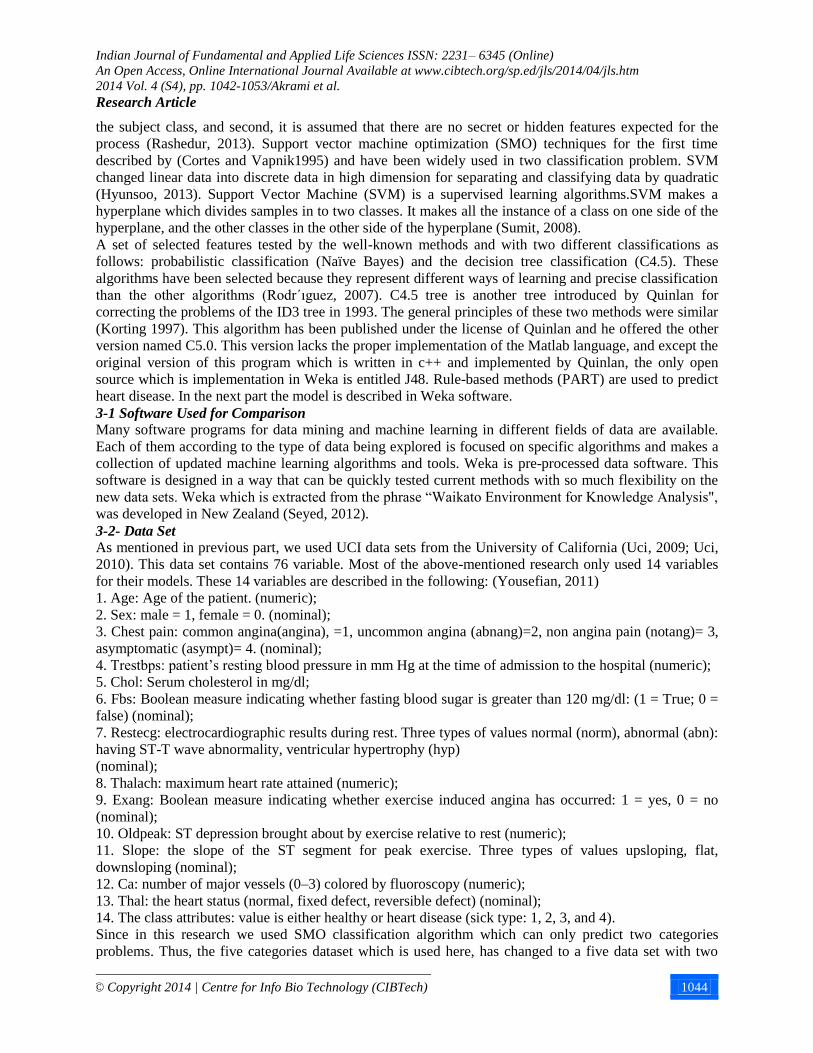
3-4- CVP 10-fold

The first step is to set the records into two categories: training with two thirds of the data and testing with

one third of the data.

Figure 3: Setup part for CVarameter Setting

Then CV parameter methods have to be used for finding optimal parameters for each of the six

classification methods with the help of 10-folding cross validation. CV parameteris in the folder of the

Meta trainer in the classification methods.

To apply this method on each of the five datasets, following steps has been done in Weka:

1- Select the Train / Test Percentage Split from the Experiment Type option.

2- Default value of the Train Percentage is 66.0.

3- Data sets are selected according to the step three in the previous part.

4- In the algorithm section, click on the Add New button to open the Choose Options and choose CV

Parameter Selection from the subfolder Meta. Then click on the Classifier to select the six classification

algorithms. 10-fold validation settings can be changed but their default values are used.

5-Other steps in this section, including the steps mentioned in the previous step will be executed and the

results of these indicators are intended to achieve.

The results of modeling on five main research datasets using CVparameter are listed in the column CVP

in Table 2.




Research Article


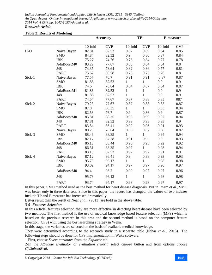
Table 2: Results of Modeling

F-measure

TP Accuracy

CVP 10-fold CVP 10-fold CVP 10-fold

0.85 0.84 0.89 0.87 82.52 82.81 Naive Bayen H-O

0.84 0.87 0.86 0.9 82.52 84.84 SMO

0.78 0.77 0.84 0.78 74.76 75.27 IBK

0.8 0.84 0.84 0.85 77.67 83.22 AdaBoostM0

0.81 0.77 0.86 0.82 78.64 74.35 J48

0.8 0.76 0.73 0.75 80.58 75.62 PART

0.87 .0.87 0.91 0.91 76.7 77.57 Naive Bayes Sick-1

0.9 0.9 1 1 82.52 81.86 SMO

0.87 0.84 0.87 0.84 78.64 74.6 IBK

0.9 0.9 1 1 82.52 81.86 AdaBoostM1

0.9 0.9 1 1 82.52 81.86 J48

087 0.85 0.88 0.87 77.67 74.54 PART

0.87 0.85 0.88 0.87 77.67 79.23 Naive Bayes Sick-2

0.94 0.93 1 1 88.35 87.8 SMO

0.87 0.9 0.86 0.9 76.7 82.53 IBK

0.94 0.92 0.99 0.95 88.35 85.81 AdaBoostM0

0.9 0.93 0.93 0.99 82.52 87.81 J48

0.93 0.91 0.96 0.92 86.41 83.54 PART

0.87 0.88 0.82 0.85 78.64 80.23 Naive Bayes

Sick-3 0.94 0.94 1 1 88.35 88.46 SMO

0.93 0.9 0.95 0.91 87.38 82.17 IBK

0.92 0.92 0.93 0.96 85.44 86.15 AdaBoostM0

0.94 0.93 1 0.97 88.35 86.51 J48

0.9 0.91 0.92 0.92 82.52 83.18 PART

0.93 0.93 0.88 0.9 86.41 87.12 Naive Bayes Sick-4

0.98 0.98 1 1 96.12 95.73 SMO

0.97 0.96 0.97 0.97 94.17 93.09 IBK

0.96 0.97 0.97 0.99 93.2 94.4 AdaBoostM0

0.98 0.98 1 1 96.12 95.73 J48

0.97 0.97 0.98 0.98 94.17 93.74 PART

In this paper, SMO method used as the best method for heart disease diagnosis. But in Imam et al., SMO

was better only in three data sets. Since in this paper, the record has changed, the values of two indexes

include TP and F-measure has increased dramatically.

Better result than the result of Near et al., (2013) are bold in the above table.

3-5- Features Selection

In this article, features selection they are more effective in detecting heart disease have been selected by

two methods. The first method is the use of medical knowledge based feature selection (MFS) which is

based on the previous research in this area and the second method is based on the computer feature

selection (CFS) with using the best searching strategy in Weka.

In this stage, the variables are selected on the basis of available medical knowledge.

They were determined according to the research study in a separate table (Nahar et al., 2013). The

following steps should be done for CFS implementation in Waka software.

1-First, choose Select attributes from the Explorer tab.

2-In the Attribute Evaluator or evaluation criteria select choose button and from options choose

CfsSubsetEval.




Research Article


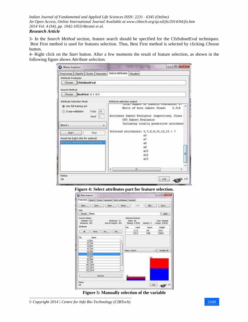
3- In the Search Method section, feature search should be specified for the CfsSubsetEval techniques.

Best First method is used for features selection. Thus, Best First method is selected by clicking Choose

button.

4- Right click on the Start button. After a few moments the result of feature selection, as shown in the

following figure shows Attribute selection.

Figure 4: Select attributes part for feature selection.

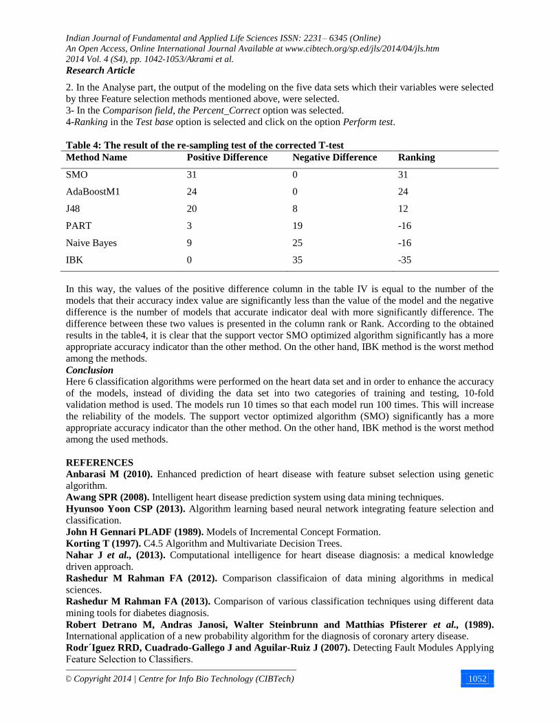
Figure 5: Manually selection of the variable




Research Article


Point: In order to select the variables manually from the Preprocess tab in Explorer and then by the

buttons Add select the variables which are not selected yet, then select the Save option at the top of the

window in order to save the changes.

Selected Variables by feature selection method based on MFS and CFS are available in five data sets.

(Nahar et al., 2013).

3-6-Modeling on the Set of Selected Variables

Here on each of the five data sets, modeling is done. By combining the selected variables, new variables

which are agreed by both methods were produced. The table 3shows the results of applying the model on

five of the six data sets, each with three methods CFS, MFS and combination of these two approaches.

Table 3: Modeling on the selected variables

F-measure TP Accuracy

MFS+CF

S

MF

S

CF

S

MFS+CF

S

MF

S

CF

S

MFS+CF

S

MFS CFS

0.85 0.76 0.86 0.87 0.76 0.88 83.01 74.2 83.9 Naive Bayen H-O

0.86 0.77 0.86 0.9 0.76 0.9 83.64 75.9

1

84.2

2

SMO

0.77 0.73 0.8 0.78 0.73 0.82 74.34 70.4

9

77.6

7

IBK

0.84 0.77 0.86 0.86 0.76 0.88 82.58 75.3

5

83.8 AdaBoostM

0

0.78 0.73 0.79 0.8 0.76 0.83 75.84 70.4

3

76.7

8

J48

0.77 0.74 0.8 0.78 0.75 0.82 75.38 72.1 77.6

6

PART

0.86 0.88 0.87 0.9 0.96 0.94 75.74 79.0

3

77.9

6

Naive Bayes Sick

-1

0.9 0.9 0.9 1 1 1 81.86 81.8

6

81.8

6

SMO

0.81 0.81 0.88 0.82 0.8 0.95 69.23 68.7

6

79.1

8

IBK

0.9 0.9 0.9 1 1 1 81.86 81.8

6

81.8

3

AdaBoostM

1

0.9 0.9 0.9 1 1 1 81.86 81.8

6

81.8

6

J48

0.83 0.87 0.89 0.86 0.95 0.99 72.28 77.7

6

80.8

1

PART

0.87 0.89 0.88 0.84 0.9 0.85 79 80.8

5

79.9 Naive Bayes Sick

-2

0.94 0.94 0.94 1 1 1 87.86 88.1

3

87.8

6

SMO

0.91 0.88 0.91 0.92 0.88 0.92 83.93 79.4

5

84.1 IBK

0.92 0.93 0.92 0.96 0.99 0.96 85.05 87.7

3

85.5

8

AdaBoostM

0




Research Article


0.93 0.93 0.93 0.98 0.99 0.99 86.61 86.9

4

87.7

7

J48

0.9 0.91 0.92 0.91 0.94 0.95 82.78 83.6

3

85.7

6

PART

0.89 0.92 0.89 0.86 0.93 0.87 81.8 85.4

9

81.9

8

Naive Bayes

Sick

-3 0.94 0.94 0.94 1 1 1 88.46 88.4

6

88.4

6

SMO

0.9 0.88 0.91 0.9 0.89 0.94 82.65 79.6

5

83.8

5

IBK

0.93 0.93 0.93 0.96 0.99 0.95 86.48 87.7 86.6

1

AdaBoostM

0

0.93 0.94 0.94 0.97 0.99 1 86.75 88 86.4

6

J48

0.91 0.92 0.93 0.92 0.96 0.97 83.41 85.6

2

86.1

8

PART

0.96 0.97 0.97 0.94 0.98 0.98 91.62 94.1

5

94.8

3

Naive Bayes Sick

-4

0.98 0.98 0.98 1 1 1 95.73 95.7

3

95.7

3

SMO

0.96 0.96 0.97 0.96 0.96 0.98 92.36 92.6

9

94.1

8

IBK

0.97 0.98 0.98 0.99 1 0.99 95.14 95.6

7

95.5 AdaBoostM

1

0.98 0.98 0.98 1 1 1 95.73 95.7

3

95.7

3

J48

0.97 0.97 0.98 0.99 0.99 1 94.44 94.8

4

95.7

3

PART

The Proposed Method

In this step, in order to raise the accuracy of the models, decision was made to rise instead of dividing the

data set into training and testing sets, 10 –fold validation method is used. And each model runs 10 times.

So each model run 100 times and this result in increasing the validity of the models. The more difference

results were marked. Validation of the data is one of the main reasons in this study. Most of the models

produced by the three feature selection methods have TP and F-measure index equal to 0 on the main data

sets in (Nahar et al., 2013). This result shows the weakness of the proposed method in over learning and

modeling but the validation of these indicators have increased dramatically.

Proposed Method for Better Evaluation

For a closer look, here, re-sample corrected T-test in order to show the difference between the

performances of the optimized support vector machine algorithm (SMO) compared to the other used

models. The test is applied based on three data sets CFS, MFS and MFS + CFS and according to the

accuracy index. In fact, this test is looked for variance between the parameters of the models, (a six

classification methods carried out on 5 datasets with 3 features selection methods that are 3 × 5 × 6 =90

models).

The following steps were implemented in Weka software:

1. The Experimenter was implemented.




Research Article


2. In the Analyse part, the output of the modeling on the five data sets which their variables were selected

by three Feature selection methods mentioned above, were selected.

3- In the Comparison field, the Percent_Correct option was selected.

4-Ranking in the Test base option is selected and click on the option Perform test.

Table 4: The result of the re-sampling test of the corrected T-test

Method Name Positive Difference Negative Difference Ranking

SMO 31 0 31

AdaBoostM1 24 0 24

J48 20 8 12

PART 3 19 -16

Naive Bayes 9 25 -16

IBK 0 35 -35

In this way, the values of the positive difference column in the table IV is equal to the number of the

models that their accuracy index value are significantly less than the value of the model and the negative

difference is the number of models that accurate indicator deal with more significantly difference. The

difference between these two values is presented in the column rank or Rank. According to the obtained

results in the table4, it is clear that the support vector SMO optimized algorithm significantly has a more

appropriate accuracy indicator than the other method. On the other hand, IBK method is the worst method

among the methods.

Conclusion

Here 6 classification algorithms were performed on the heart data set and in order to enhance the accuracy

of the models, instead of dividing the data set into two categories of training and testing, 10-fold

validation method is used. The models run 10 times so that each model run 100 times. This will increase

the reliability of the models. The support vector optimized algorithm (SMO) significantly has a more

appropriate accuracy indicator than the other method. On the other hand, IBK method is the worst method

among the used methods.

REFERENCES

Anbarasi M (2010). Enhanced prediction of heart disease with feature subset selection using genetic

algorithm.

Awang SPR (2008). Intelligent heart disease prediction system using data mining techniques.

Hyunsoo Yoon CSP (2013). Algorithm learning based neural network integrating feature selection and

classification.

John H Gennari PLADF (1989). Models of Incremental Concept Formation.

Korting T (1997). C4.5 Algorithm and Multivariate Decision Trees.

Nahar J et al., (2013). Computational intelligence for heart disease diagnosis: a medical knowledge

driven approach.

Rashedur M Rahman FA (2012). Comparison classificaion of data mining algorithms in medical

sciences.

Rashedur M Rahman FA (2013). Comparison of various classification techniques using different data

mining tools for diabetes diagnosis.

Robert Detrano M, Andras Janosi, Walter Steinbrunn and Matthias Pfisterer et al., (1989). International application of a new probability algorithm for the diagnosis of coronary artery disease.

Rodr´Iguez RRD, Cuadrado-Gallego J and Aguilar-Ruiz J (2007). Detecting Fault Modules Applying

Feature Selection to Classifiers.




Research Article


Seyed Abbas Mahmoodi MSM (2012). Assessment of classification algorithms in the diagnosis of

diabetes and breast cancer.

Shahrabi JZSA (2009). Advanced data mining: concepts and algorithms, Tehran, Jahad Daneshgahi

algorithms.

Sumit Bhatia PP and Pillai GN (2008). Svm based decision support system for heart disease

classification with integer-coded genetic algorithm to select critical features.

Uci (2009). Heart Disease Dataset [Online].

Wasan HKASK (2006). Empirical study on applications of data mining techniques in healthcare.

Yousefian VAA (2011). Data Mining Techniques used to Diagnose Heart Disease, edited by Vahid

Asaeedi and Alireza Yousefian.

Documents

APPLICATION OF COMPUTATIONAL INTELLIGENCE IN · PDF file · 2014-12-14Indian Journal of Fundamental and Applied Life Sciences ISSN: 2231– 6345 (Online) An Open Access, Online International