Application of 4K-QAM, LDPC and OFDM for Gbps Data Rates over HFC Plant

David John Urban Comcast

Abstract This paper describes the application of

4096-QAM, low density parity check codes

(LDPC), and orthogonal frequency division

multiplexing (OFDM) to transmission over a

hybrid fiber coaxial cable plant (HFC). These

techniques enable data rates of several Gbps.

A complete derivation of the equations

used for log domain sum product LDPC

decoding is provided. The reasons for

selecting OFDM and 4K-QAM are described.

Analysis of performance in the presence of

noise taken from field measurements is made.

INTRODUCTION A new physical layer is being developed for transmission of data over a HFC cable plant. The objective is to increase the HFC plant capacity. A straightforward method to increase capacity over the HFC plant is to allocate more spectrum.The spectrum used for RF signals is typically 5-42 MHz in the upstream and 54-750 MHz in the downstream for HFC plants in the United States, although many variations of the upstream and downstream frequency allocations exist. The downstream signals can be extended to 1002 MHz to increase downstream capacity. The upstream can be increased to 5-85 MHz or even higher to increase upstream capacity. The capacity can be increased with higher spectral efficiency, the bits per second in a Hz of bandwidth. The capacity can be increased by packing more signals into existing spectrum, for example by reducing loss due to filter rolloffs, and adding more robust signals that can work in noisy parts of the spectrum.

Higher spectral density requires mapping more bits into a symbol at the expense of a higher signal to noise ratio (SNR) threshold. The new physical layer will map 12 bits per symbol on the downstream compared to the 8 bits per symbol used in DOCSIS 3.0. 4K-QAM (or 4096-QAM) is a modulation technique that has 4,096 points in the constellation diagram and each point is mapped to 12 bits. The new physical layer will map 10 bits per symbol using 1024-QAM (or 1K-QAM) on the upstream compared to 6 bits per symbol with 64-QAM used in DOCSIS 3.0.

INCREASING SPECTRAL EFFICIENCY The three key methods for increasing the spectral efficiency of the HFC plant in the new physical layer are LDPC, OFDM and 4K-QAM. LDPC is a very efficient coding scheme. OFDM divides the spectrum into small subcarriers. 4K-QAM maps each symbol into 12 bits. LDPC is a linear block code that utilizes a sparse parity check matrix. Since the parity check matrix is sparse, the code word can be very long with a reasonable calculation complexity. With a long code word size the parity check equations can have statistically significant samples. This allows LDPC codes to be demodulated with an iterative message passing algorithm based upon the log-likelihood ratio (LLR) for each bit of the code word. The data rate is calculated by multiplying the spectral efficiency by the channel width, so the data rate can be doubled by doubling the channel width. A wide channel width results in a short symbol period; this increases the length of the adaptive equalizer needed to

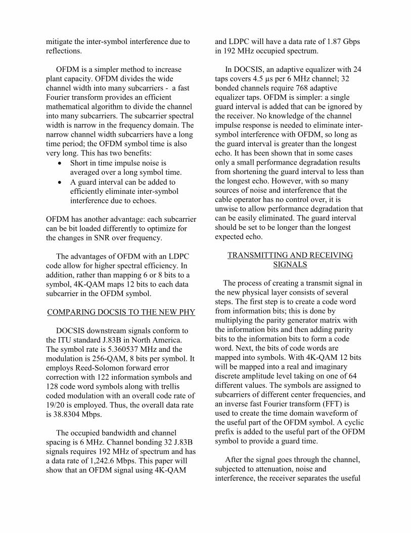
mitigate the inter-symbol interference due to reflections. OFDM is a simpler method to increase plant capacity. OFDM divides the wide channel width into many subcarriers - a fast Fourier transform provides an efficient mathematical algorithm to divide the channel into many subcarriers. The subcarrier spectral width is narrow in the frequency domain. The narrow channel width subcarriers have a long time period; the OFDM symbol time is also very long. This has two benefits:

Short in time impulse noise is averaged over a long symbol time.

A guard interval can be added to efficiently eliminate inter-symbol interference due to echoes.

OFDM has another advantage: each subcarrier can be bit loaded differently to optimize for the changes in SNR over frequency. The advantages of OFDM with an LDPC code allow for higher spectral efficiency. In addition, rather than mapping 6 or 8 bits to a symbol, 4K-QAM maps 12 bits to each data subcarrier in the OFDM symbol. COMPARING DOCSIS TO THE NEW PHY DOCSIS downstream signals conform to the ITU standard J.83B in North America. The symbol rate is 5.360537 MHz and the modulation is 256-QAM, 8 bits per symbol. It employs Reed-Solomon forward error correction with 122 information symbols and 128 code word symbols along with trellis coded modulation with an overall code rate of 19/20 is employed. Thus, the overall data rate is 38.8304 Mbps. The occupied bandwidth and channel spacing is 6 MHz. Channel bonding 32 J.83B signals requires 192 MHz of spectrum and has a data rate of 1,242.6 Mbps. This paper will show that an OFDM signal using 4K-QAM

and LDPC will have a data rate of 1.87 Gbps in 192 MHz occupied spectrum. In DOCSIS, an adaptive equalizer with 24 taps covers 4.5 µs per 6 MHz channel; 32 bonded channels require 768 adaptive equalizer taps. OFDM is simpler: a single guard interval is added that can be ignored by the receiver. No knowledge of the channel impulse response is needed to eliminate inter-symbol interference with OFDM, so long as the guard interval is greater than the longest echo. It has been shown that in some cases only a small performance degradation results from shortening the guard interval to less than the longest echo. However, with so many sources of noise and interference that the cable operator has no control over, it is unwise to allow performance degradation that can be easily eliminated. The guard interval should be set to be longer than the longest expected echo.

TRANSMITTING AND RECEIVING SIGNALS

The process of creating a transmit signal in the new physical layer consists of several steps. The first step is to create a code word from information bits; this is done by multiplying the parity generator matrix with the information bits and then adding parity bits to the information bits to form a code word. Next, the bits of code words are mapped into symbols. With 4K-QAM 12 bits will be mapped into a real and imaginary discrete amplitude level taking on one of 64 different values. The symbols are assigned to subcarriers of different center frequencies, and an inverse fast Fourier transform (FFT) is used to create the time domain waveform of the useful part of the OFDM symbol. A cyclic prefix is added to the useful part of the OFDM symbol to provide a guard time. After the signal goes through the channel, subjected to attenuation, noise and interference, the receiver separates the useful

symbol period from the cyclic prefix. An FFT of the time domain useful symbol period outputs in-phase (I) and quadrature (Q) received vectors for each data subcarrier. From the received vectors, log-likelihood ratios (LLRs) of each bit in the code word are determined and passed on to the LDPC decoder. The LDPC decoder uses a message passing algorithm between check nodes and variable nodes to iteratively converge on the transmitted code word. Received signals are degraded by three types of noise: thermal, ingress and impulse. Thermal noise is flat over frequency, determined by the receiver noise figure and the input level. Ingress noise is narrow in frequency and long in time, mostly due to radio interference. New cellular services based on LTE are particularly worrisome since they are typically 10 MHz wide and operate co-channel with HFC downstream frequencies. Impulse noise is narrow in time but wide in frequency; the most common source being electrical systems such as motors and lighting systems. The downstream receive signals are dominated by thermal and ingress noise, while the upstream received signals have all three types. The downstream is higher in frequency, so cable attenuation is higher and thermal noise is more of a problem. Impulse noise can be observed at downstream frequencies, but tends to be less prevalent than ingress interference. Radio interference from broadcast, cellular, and public safety impact downstream signal quality. On the upstream impulse noise has very high amplitudes below 20 MHz. Radio interference from shortwave, amateur, and citizen's band services are also major interferers.

NEW PHY DETAILS

The following sections of the paper describe the components of the new PHY: 4K-QAM, OFDM, and LDPC. The LDPC section includes a complete derivation of equations used for decoding an LDPC signal. After the LDPC section, a section on performance analysis provides results of simulations using field measured noise.

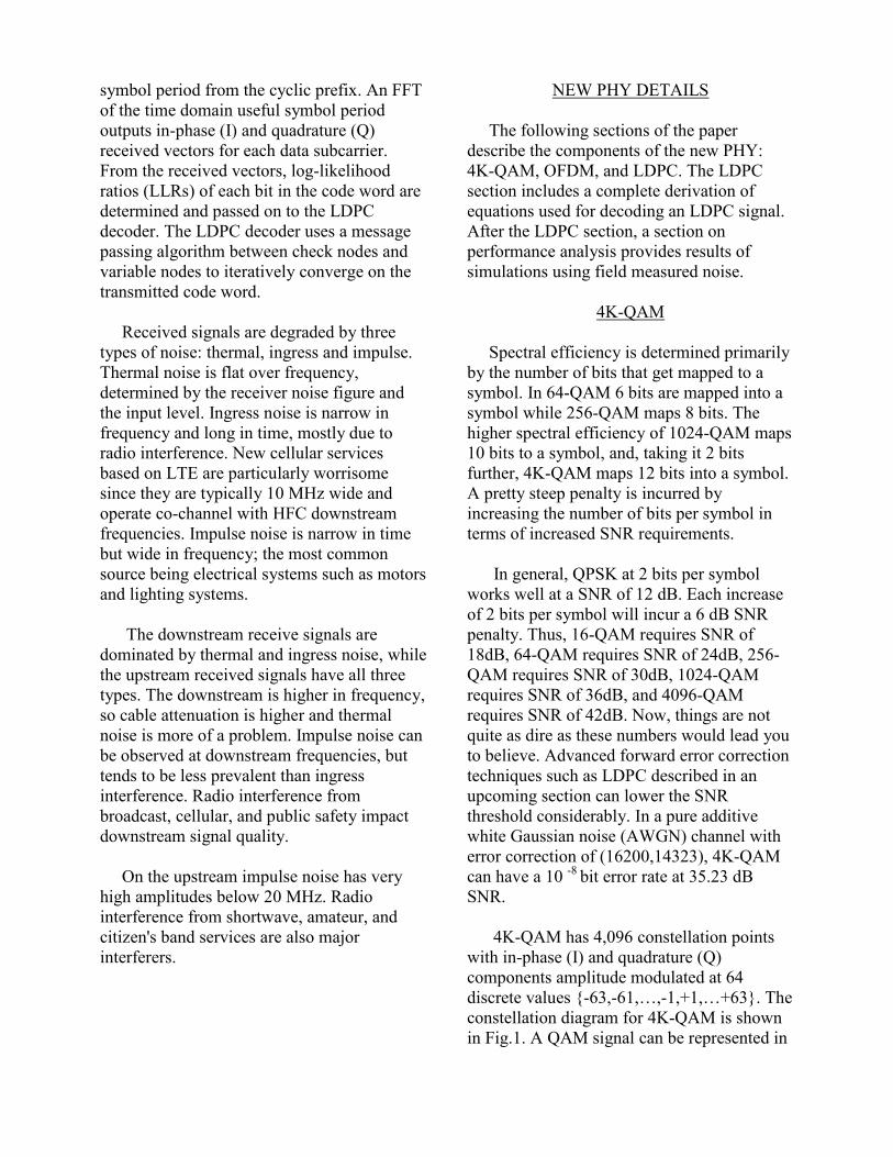
4K-QAM Spectral efficiency is determined primarily by the number of bits that get mapped to a symbol. In 64-QAM 6 bits are mapped into a symbol while 256-QAM maps 8 bits. The higher spectral efficiency of 1024-QAM maps 10 bits to a symbol, and, taking it 2 bits further, 4K-QAM maps 12 bits into a symbol. A pretty steep penalty is incurred by increasing the number of bits per symbol in terms of increased SNR requirements. In general, QPSK at 2 bits per symbol works well at a SNR of 12 dB. Each increase of 2 bits per symbol will incur a 6 dB SNR penalty. Thus, 16-QAM requires SNR of 18dB, 64-QAM requires SNR of 24dB, 256-QAM requires SNR of 30dB, 1024-QAM requires SNR of 36dB, and 4096-QAM requires SNR of 42dB. Now, things are not quite as dire as these numbers would lead you to believe. Advanced forward error correction techniques such as LDPC described in an upcoming section can lower the SNR threshold considerably. In a pure additive white Gaussian noise (AWGN) channel with error correction of (16200,14323), 4K-QAM can have a 10 -8 bit error rate at 35.23 dB SNR. 4K-QAM has 4,096 constellation points with in-phase (I) and quadrature (Q) components amplitude modulated at 64 discrete values {-63,-61,…,-1,+1,…+63}. The constellation diagram for 4K-QAM is shown in Fig.1. A QAM signal can be represented in

complex form as I+jQ where j is the square root of minus 1. I is the in-phase or real part of the complex baseband signal and Q is the quadrature or imaginary part of the complex baseband signal. The modulated signal is I(t)cos(2πft)+Q(t)sin(2πft).

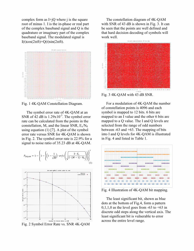
Fig. 1 4K-QAM Constellation Diagram. The symbol error rate of 4K-QAM at an SNR of 42 dB is 1.29x10-3. The symbol error rate can be calculated from the points in the constellation, M, and the linear SNR, Es/N0 using equation (1) [7]. A plot of the symbol error rate versus SNR for 4K-QAM is shown in Fig. 2. The symbol error rate is 22.9% for a signal to noise ratio of 35.23 dB at 4K-QAM.

(1)

Fig. 2 Symbol Error Rate vs. SNR 4K-QAM

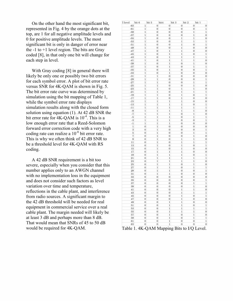
The constellation diagram of 4K-QAM with SNR of 43 dB is shown in Fig. 3. It can be seen that the points are well defined and that hard decision decoding of symbols will work well.

Fig. 3 4K-QAM with 43 dB SNR. For a modulation of 4K-QAM the number of constellation points is 4096 and each symbol is mapped to 12 bits. 6 bits are mapped to an I value and the other 6 bits are mapped to a Q value. The I and Q levels are selected from the range of odd numbers between -63 and +63. The mapping of bits into I and Q levels for 4K-QAM is illustrated in Fig. 4 and listed in Table 1.

Fig. 4 Illustration of 4K-QAM bit mapping. The least significant bit, shown as blue dots at the bottom of Fig.4, form a pattern 0,1,1,0 as the level goes from -63 to +63 in discrete odd steps along the vertical axis. The least significant bit is vulnerable to error across the entire level range.

On the other hand the most significant bit, represented in Fig. 4 by the orange dots at the top, are 1 for all negative amplitude levels and 0 for positive amplitude levels. The most significant bit is only in danger of error near the -1 to +1 level region. The bits are Gray coded [8], in that only one bit will change for each step in level. With Gray coding [8] in general there will likely be only one or possibly two bit errors for each symbol error. A plot of bit error rate versus SNR for 4K-QAM is shown in Fig. 5. The bit error rate curve was determined by simulation using the bit mapping of Table 1, while the symbol error rate displays simulation results along with the closed form solution using equation (1). At 42 dB SNR the bit error rate for 4K-QAM is 10-4. This is a low enough error rate that a Reed-Solomon forward error correction code with a very high coding rate can realize a 10-8 bit error rate. This is why we often think of 42 dB SNR to be a threshold level for 4K-QAM with RS coding. A 42 dB SNR requirement is a bit too severe, especially when you consider that this number applies only to an AWGN channel with no implementation loss in the equipment and does not consider such factors as level variation over time and temperature, reflections in the cable plant, and interference from radio sources. A significant margin to the 42 dB threshold will be needed for real equipment in commercial service over a real cable plant. The margin needed will likely be at least 3 dB and perhaps more than 8 dB. That would mean that SNRs of 45 to 50 dB would be required for 4K-QAM.

Table 1. 4K-QAM Mapping Bits to I/Q Level.

I level bit 6 bit 5 bit4 bit 3 bit 2 bit 1

-63 1 0 0 0 0 0

-61 1 0 0 0 0 1

-59 1 0 0 0 1 1

-57 1 0 0 0 1 0

-55 1 0 0 1 1 0

-53 1 0 0 1 1 1

-51 1 0 0 1 0 1

-49 1 0 0 1 0 0

-47 1 0 1 1 0 0

-45 1 0 1 1 0 1

-43 1 0 1 1 1 1

-41 1 0 1 1 1 0

-39 1 0 1 0 1 0

-37 1 0 1 0 1 1

-35 1 0 1 0 0 1

-33 1 0 1 0 0 0

-31 1 1 0 0 0 0

-29 1 1 0 0 0 1

-27 1 1 0 0 1 1

-25 1 1 0 0 1 0

-23 1 1 0 1 1 0

-21 1 1 0 1 1 1

-19 1 1 0 1 0 1

-17 1 1 0 1 0 0

-15 1 1 1 1 0 0

-13 1 1 1 1 0 1

-11 1 1 1 1 1 1

-9 1 1 1 1 1 0

-7 1 1 1 0 1 0

-5 1 1 1 0 1 1

-3 1 1 1 0 0 1

-1 1 1 1 0 0 0

1 0 1 0 0 0 0

3 0 1 0 0 0 1

5 0 1 0 0 1 1

7 0 1 0 0 1 0

9 0 1 0 1 1 0

11 0 1 0 1 1 1

13 0 1 0 1 0 1

15 0 1 0 1 0 0

17 0 1 1 1 0 0

19 0 1 1 1 0 1

21 0 1 1 1 1 1

23 0 1 1 1 1 0

25 0 1 1 0 1 0

27 0 1 1 0 1 1

29 0 1 1 0 0 1

31 0 1 1 0 0 0

33 0 0 0 0 0 0

35 0 0 0 0 0 1

37 0 0 0 0 1 1

39 0 0 0 0 1 0

41 0 0 0 1 1 0

43 0 0 0 1 1 1

45 0 0 0 1 0 1

47 0 0 0 1 0 0

49 0 0 1 1 0 0

51 0 0 1 1 0 1

53 0 0 1 1 1 1

55 0 0 1 1 1 0

57 0 0 1 0 1 0

59 0 0 1 0 1 1

61 0 0 1 0 0 1

63 0 0 1 0 0 0

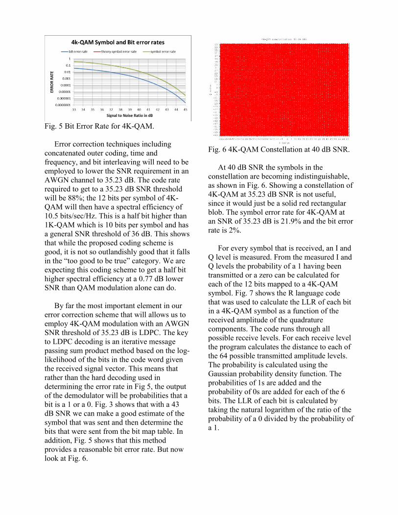
Fig. 5 Bit Error Rate for 4K-QAM. Error correction techniques including concatenated outer coding, time and frequency, and bit interleaving will need to be employed to lower the SNR requirement in an AWGN channel to 35.23 dB. The code rate required to get to a 35.23 dB SNR threshold will be 88%; the 12 bits per symbol of 4K-QAM will then have a spectral efficiency of 10.5 bits/sec/Hz. This is a half bit higher than 1K-QAM which is 10 bits per symbol and has a general SNR threshold of 36 dB. This shows that while the proposed coding scheme is good, it is not so outlandishly good that it falls in the “too good to be true” category. We are expecting this coding scheme to get a half bit higher spectral efficiency at a 0.77 dB lower SNR than QAM modulation alone can do. By far the most important element in our error correction scheme that will allows us to employ 4K-QAM modulation with an AWGN SNR threshold of 35.23 dB is LDPC. The key to LDPC decoding is an iterative message passing sum product method based on the log-likelihood of the bits in the code word given the received signal vector. This means that rather than the hard decoding used in determining the error rate in Fig 5, the output of the demodulator will be probabilities that a bit is a 1 or a 0. Fig. 3 shows that with a 43 dB SNR we can make a good estimate of the symbol that was sent and then determine the bits that were sent from the bit map table. In addition, Fig. 5 shows that this method provides a reasonable bit error rate. But now look at Fig. 6.

Fig. 6 4K-QAM Constellation at 40 dB SNR. At 40 dB SNR the symbols in the constellation are becoming indistinguishable, as shown in Fig. 6. Showing a constellation of 4K-QAM at 35.23 dB SNR is not useful, since it would just be a solid red rectangular blob. The symbol error rate for 4K-QAM at an SNR of 35.23 dB is 21.9% and the bit error rate is 2%. For every symbol that is received, an I and Q level is measured. From the measured I and Q levels the probability of a 1 having been transmitted or a zero can be calculated for each of the 12 bits mapped to a 4K-QAM symbol. Fig. 7 shows the R language code that was used to calculate the LLR of each bit in a 4K-QAM symbol as a function of the received amplitude of the quadrature components. The code runs through all possible receive levels. For each receive level the program calculates the distance to each of the 64 possible transmitted amplitude levels. The probability is calculated using the Gaussian probability density function. The probabilities of 1s are added and the probability of 0s are added for each of the 6 bits. The LLR of each bit is calculated by taking the natural logarithm of the ratio of the probability of a 0 divided by the probability of a 1.

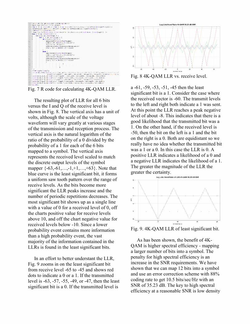
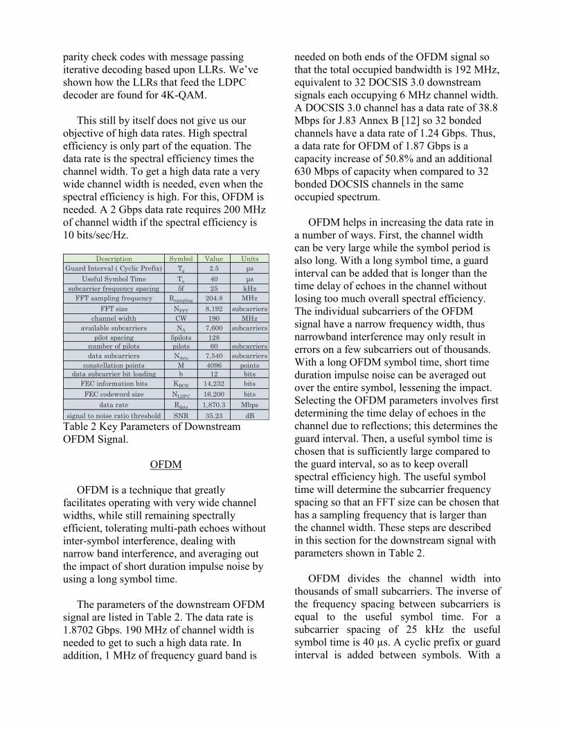
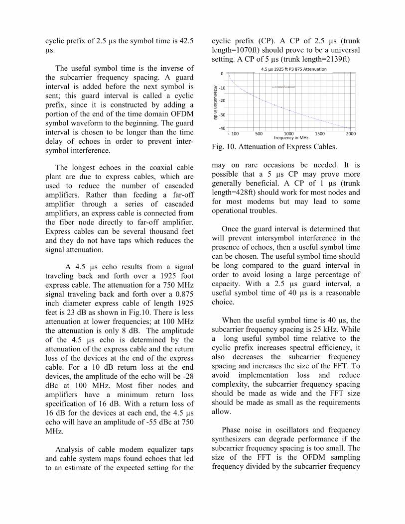
Fig. 7 R code for calculating 4K-QAM LLR. The resulting plot of LLR for all 6 bits versus the I and Q of the receive level is shown in Fig. 8. The vertical axis has a unit of volts, although the scale of the voltage waveform will vary greatly at various stages of the transmission and reception process. The vertical axis is the natural logarithm of the ratio of the probability of a 0 divided by the probability of a 1 for each of the 6 bits mapped to a symbol. The vertical axis represents the received level scaled to match the discrete output levels of the symbol mapper {-63,-61,…,-1,+1,…,+63}. Note that blue curve is the least significant bit, it forms a uniform saw tooth pattern over the range of receive levels. As the bits become more significant the LLR peaks increase and the number of periodic repetitions decreases. The most significant bit shows up as a single line with a value of 0 for a received level of 0, off the charts positive value for receive levels above 10, and off the chart negative value for received levels below -10. Since a lower probability event contains more information than a high probability event, the vast majority of the information contained in the LLRs is found in the least significant bits. In an effort to better understant the LLR, Fig. 9 zooms in on the least significant bit from receive level -65 to -45 and shows red dots to indicate a 0 or a 1. If the transmitted level is -63, -57, -55, -49, or -47, then the least significant bit is a 0. If the transmitted level is

Fig. 8 4K-QAM LLR vs. receive level. a -61, -59, -53, -51, -45 then the least significant bit is a 1. Consider the case where the received vector is -60. The transmit levels to the left and right both indicate a 1 was sent. At this point the LLR reaches a peak negative level of about -8. This indicates that there is a good likelihood that the transmitted bit was a 1. On the other hand, if the received level is -50, then the bit on the left is a 1 and the bit on the right is a 0. Both are equidistant so we really have no idea whether the transmitted bit was a 1 or a 0. In this case the LLR is 0. A positive LLR indicates a likelihood of a 0 and a negative LLR indicates the likelihood of a 1. The greater the magnitude of the LLR the greater the certainty.

Fig. 9. 4K-QAM LLR of least significant bit. As has been shown, the benefit of 4K-QAM is higher spectral efficiency - mapping a larger number of bits into a symbol. The penalty for high spectral efficiency is an increase in the SNR requirements. We have shown that we can map 12 bits into a symbol and use an error correction scheme with 88% coding rate to get 10.5 bits/sec/Hz with an SNR of 35.23 dB. The key to high spectral efficiency at a reasonable SNR is low density

parity check codes with message passing iterative decoding based upon LLRs. We’ve shown how the LLRs that feed the LDPC decoder are found for 4K-QAM. This still by itself does not give us our objective of high data rates. High spectral efficiency is only part of the equation. The data rate is the spectral efficiency times the channel width. To get a high data rate a very wide channel width is needed, even when the spectral efficiency is high. For this, OFDM is needed. A 2 Gbps data rate requires 200 MHz of channel width if the spectral efficiency is 10 bits/sec/Hz.

Table 2 Key Parameters of Downstream OFDM Signal.

OFDM

OFDM is a technique that greatly facilitates operating with very wide channel widths, while still remaining spectrally efficient, tolerating multi-path echoes without inter-symbol interference, dealing with narrow band interference, and averaging out the impact of short duration impulse noise by using a long symbol time. The parameters of the downstream OFDM signal are listed in Table 2. The data rate is 1.8702 Gbps. 190 MHz of channel width is needed to get to such a high data rate. In addition, 1 MHz of frequency guard band is

needed on both ends of the OFDM signal so that the total occupied bandwidth is 192 MHz, equivalent to 32 DOCSIS 3.0 downstream signals each occupying 6 MHz channel width. A DOCSIS 3.0 channel has a data rate of 38.8 Mbps for J.83 Annex B [12] so 32 bonded channels have a data rate of 1.24 Gbps. Thus, a data rate for OFDM of 1.87 Gbps is a capacity increase of 50.8% and an additional 630 Mbps of capacity when compared to 32 bonded DOCSIS channels in the same occupied spectrum. OFDM helps in increasing the data rate in a number of ways. First, the channel width can be very large while the symbol period is also long. With a long symbol time, a guard interval can be added that is longer than the time delay of echoes in the channel without losing too much overall spectral efficiency. The individual subcarriers of the OFDM signal have a narrow frequency width, thus narrowband interference may only result in errors on a few subcarriers out of thousands. With a long OFDM symbol time, short time duration impulse noise can be averaged out over the entire symbol, lessening the impact. Selecting the OFDM parameters involves first determining the time delay of echoes in the channel due to reflections; this determines the guard interval. Then, a useful symbol time is chosen that is sufficiently large compared to the guard interval, so as to keep overall spectral efficiency high. The useful symbol time will determine the subcarrier frequency spacing so that an FFT size can be chosen that has a sampling frequency that is larger than the channel width. These steps are described in this section for the downstream signal with parameters shown in Table 2. OFDM divides the channel width into thousands of small subcarriers. The inverse of the frequency spacing between subcarriers is equal to the useful symbol time. For a subcarrier spacing of 25 kHz the useful symbol time is 40 µs. A cyclic prefix or guard interval is added between symbols. With a

Description Symbol Value Units

Guard Interval ( Cyclic Prefix) Tg 2.5 μs

Useful Symbol Time Tu 40 μs

subcarrier frequency spacing δf 25 kHz

FFT sampling frequency Rsampling 204.8 MHz

FFT size NFFT 8,192 subcarriers

channel width CW 190 MHz

available subcarriers NA 7,600 subcarriers

pilot spacing δpilots 128

number of pilots pilots 60 subcarriers

data subcarriers Ndata 7,540 subcarriers

constellation points M 4096 points

data subcarrier bit loading b 12 bits

FEC information bits KBCH 14,232 bits

FEC codeword size NLDPC 16,200 bits

data rate Rdata 1,870.3 Mbps

signal to noise ratio threshold SNR 35.23 dB

cyclic prefix of 2.5 µs the symbol time is 42.5 µs. The useful symbol time is the inverse of the subcarrier frequency spacing. A guard interval is added before the next symbol is sent; this guard interval is called a cyclic prefix, since it is constructed by adding a portion of the end of the time domain OFDM symbol waveform to the beginning. The guard interval is chosen to be longer than the time delay of echoes in order to prevent inter-symbol interference.

The longest echoes in the coaxial cable plant are due to express cables, which are used to reduce the number of cascaded amplifiers. Rather than feeding a far-off amplifier through a series of cascaded amplifiers, an express cable is connected from the fiber node directly to far-off amplifier. Express cables can be several thousand feet and they do not have taps which reduces the signal attenuation.

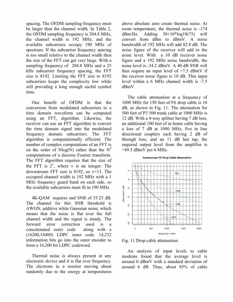
A 4.5 µs echo results from a signal traveling back and forth over a 1925 foot express cable. The attenuation for a 750 MHz signal traveling back and forth over a 0.875 inch diameter express cable of length 1925 feet is 23 dB as shown in Fig.10. There is less attenuation at lower frequencies; at 100 MHz the attenuation is only 8 dB. The amplitude of the 4.5 µs echo is determined by the attenuation of the express cable and the return loss of the devices at the end of the express cable. For a 10 dB return loss at the end devices, the amplitude of the echo will be -28 dBc at 100 MHz. Most fiber nodes and amplifiers have a minimum return loss specification of 16 dB. With a return loss of 16 dB for the devices at each end, the 4.5 µs echo will have an amplitude of -55 dBc at 750 MHz. Analysis of cable modem equalizer taps and cable system maps found echoes that led to an estimate of the expected setting for the

cyclic prefix (CP). A CP of 2.5 µs (trunk length=1070ft) should prove to be a universal setting. A CP of 5 µs (trunk length=2139ft)

Fig. 10. Attenuation of Express Cables. may on rare occasions be needed. It is possible that a 5 µs CP may prove more generally beneficial. A CP of 1 µs (trunk length=428ft) should work for most nodes and for most modems but may lead to some operational troubles. Once the guard interval is determined that will prevent intersymbol interference in the presence of echoes, then a useful symbol time can be chosen. The useful symbol time should be long compared to the guard interval in order to avoid losing a large percentage of capacity. With a 2.5 µs guard interval, a useful symbol time of 40 µs is a reasonable choice. When the useful symbol time is 40 µs, the subcarrier frequency spacing is 25 kHz. While a long useful symbol time relative to the cyclic prefix increases spectral efficiency, it also decreases the subcarrier frequency spacing and increases the size of the FFT. To avoid implementation loss and reduce complexity, the subcarrier frequency spacing should be made as wide and the FFT size should be made as small as the requirements allow. Phase noise in oscillators and frequency synthesizers can degrade performance if the subcarrier frequency spacing is too small. The size of the FFT is the OFDM sampling frequency divided by the subcarrier frequency

frequency in MHz

4.5 µs 1925 ft P3 875 Attenuation

Atten

uatio

n in

dB

-10

0

-20

-30

-40100 500 1000 1500 2000

spacing. The OFDM sampling frequency must be larger than the channel width. In Table 2, the OFDM sampling frequency is 204.8 MHz, the channel width is 192 MHz, and the available subcarriers occupy 190 MHz of spectrum. If the subcarrier frequency spacing is too small relative to the channel width then the size of the FFT can get very large. With a sampling frequency of 204.8 MHz and a 25 kHz subcarrier frequency spacing, the FFT size is 8192. Limiting the FFT size to 8192 subcarriers keeps the complexity low while still providing a long enough useful symbol time. One benefit of OFDM is that the conversion from modulated subcarriers to a time domain waveform can be computed using an FFT, algorithm. Likewise, the receiver can use an FFT algorithm to convert the time domain signal into the modulated frequency domain subcarriers. The FFT algorithm is computationally efficient. The number of complex computations of an FFT is on the order of Nlog(N) rather than the N2 computations of a discrete Fourier transform. The FFT algorithm requires that the size of the FFT is 2, where is an integer. The downstream FFT size is 8192, so =13. The occupied channel width is 192 MHz with a 1 MHz frequency guard band on each side, so the available subcarriers must fit in 190 MHz. 4K-QAM requires and SNR of 35.23 dB. The channel for this SNR threshold is AWGN, additive white Gaussian noise, which means that the noise is flat over the full channel width and the signal is steady. The forward error correction used is a concatenated outer code along with a (16200,14400) LDPC inner code. 14,232 information bits go into the outer encoder to form a 16,200 bit LDPC codeword. Thermal noise is always present in any electronic device and it is flat over frequency. The electrons in a resistor moving about randomly due to the energy at temperatures

above absolute zero create thermal noise. At room temperature, the thermal noise is -174 dBm/Hz. Adding 30+10*log10(75) will convert from dBm to dBmV. A noise bandwidth of 192 MHz will add 82.8 dB. The noise figure of the receiver will add to the noise level. With a 10 dB receiver noise figure and a 192 MHz noise bandwidth, the noise level is -34.2 dBmV. A 40 dB SNR will thus require an input level of +7.5 dBmV if the receiver noise figure is 10 dB. This input level within a 6 MHz channel width is -7.5 dBmV. The cable attenuation at a frequency of 1000 MHz for 150 feet of F6 drop cable is 10 dB, as shown in Fig. 11. The attenuation for 500 feet of P3 500 trunk cable at 1000 MHz is 12 dB. With a 4-way splitter having 7 dB loss, an additional 100 feet of in home cable having a loss of 7 dB at 1000 MHz, five in line directional couplers each having 2 dB of through loss, and an 11 dB last tap, the required output level from the amplifier is +49.5 dBmV per 6 MHz.

Fig. 11 Drop cable attenuation. An analysis of input levels to cable modems found that the average level is around 0 dBmV with a standard deviation of around 6 dB. Thus, about 85% of cable

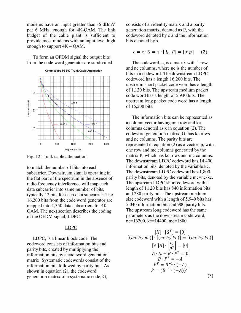
modems have an input greater than -6 dBmV per 6 MHz, enough for 4K-QAM. The link budget of the cable plant is sufficient to provide most modems with an input level high enough to support 4K – QAM. To form an OFDM signal the output bits from the code word generator are subdivided

Fig. 12 Trunk cable attenuation. to match the number of bits into each subcarrier. Downstream signals operating in the flat part of the spectrum in the absence of radio frequency interference will map each data subcarrier into same number of bits, typically 12 bits for each data subcarrier. The 16,200 bits from the code word generator are mapped into 1,350 data subcarriers for 4K-QAM. The next section describes the coding of the OFDM signal, LDPC.

LDPC LDPC, is a linear block code. The codeword consists of information bits and parity bits, created by multiplying the information bits by a codeword generation matrix. Systematic codewords consist of the information bits followed by parity bits. As shown in equation (2), the codeword generation matrix of a systematic code, G,

consists of an identity matrix and a parity generation matrix, denoted as P, with the codeword denoted by c and the information bits denoted by x.

The codeword, c, is a matrix with 1 row and nc columns, where nc is the number of bits in a codeword. The downstream LDPC codeword has a length 16,200 bits. The upstream short packet code word has a length of 1,120 bits. The upstream medium packet code word has a length of 5,940 bits. The upstream long packet code word has a length of 16,200 bits. The information bits can be represented as a column vector having one row and kc columns denoted as x in equation (2). The codeword generation matrix, G, has kc rows and nc columns. The parity bits are represented in equation (2) as a vector, p, with one row and mc columns generated by the matrix P, which has kc rows and mc columns. The downstream LDPC codeword has 14,400 information bits, denoted by the variable kc. The downstream LDPC codeword has 1,800 parity bits, denoted by the variable mc=nc-kc. The upstream LDPC short codeword with a length of 1,120 bits has 840 information bits and 280 parity bits. The upstream medium size codeword with a length of 5,940 bits has 5,040 information bits and 900 parity bits. The upstream long codeword has the same parameters as the downstream code word, nc=16200, kc=14400, mc=1800.

(3)

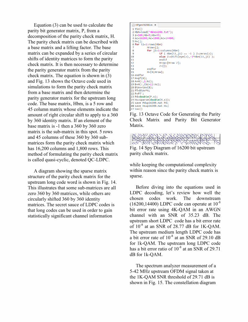
Equation (3) can be used to calculate the parity bit generator matrix, P, from a decomposition of the parity check matrix, H. The parity check matrix can be described with a base matrix and a lifting factor. The base matrix can be expanded by a series of circular shifts of identity matrices to form the parity check matrix. It is then necessary to determine the parity generator matrix from the parity check matrix. The equation is shown in (3) and Fig. 13 shows the Octave code used in simulations to form the parity check matrix from a base matrix and then determine the parity generator matrix for the upstream long code. The base matrix, Hbm, is a 5 row and 45 column matrix whose elements indicate the amount of right circular shift to apply to a 360 by 360 identity matrix. If an element of the base matrix is -1 then a 360 by 360 zero matrix is the sub-matrix in this spot. 5 rows and 45 columns of these 360 by 360 sub-matrices form the parity check matrix which has 16,200 columns and 1,800 rows. This method of formulating the parity check matrix is called quasi-cyclic, denoted QC-LDPC. A diagram showing the sparse matrix structure of the parity check matrix for the upstream long code word is shown in Fig. 14. This illustrates that some sub-matrices are all zero 360 by 360 matrices, while others are circularly shifted 360 by 360 identity matrices. The secret sauce of LDPC codes is that long codes can be used in order to gain statistically significant channel information

Fig. 13 Octave Code for Generating the Parity Check Matrix and Parity Bit Generator Matrix.

Fig. 14 Spy Diagram of 16200 bit upstream parity check matrix. while keeping the computational complexity within reason since the parity check matrix is sparse. Before diving into the equations used in LDPC decoding, let’s review how well the chosen codes work. The downstream (16200,14400) LDPC code can operate at 10-8 bit error rate using 4K-QAM in an AWGN channel with an SNR of 35.23 dB. The upstream short LDPC code has a bit error rate of 10-8 at an SNR of 28.77 dB for 1K-QAM. The upstream medium length LDPC code has a bit error rate of 10-8 at an SNR of 29.10 dB for 1k-QAM. The upstream long LDPC code has a bit error ratio of 10-8 at an SNR of 29.71 dB for 1k-QAM. The spectrum analyzer measurement of a 5-42 MHz upstream OFDM signal taken at the 1K-QAM SNR threshold of 29.71 dB is shown in Fig. 15. The constellation diagram

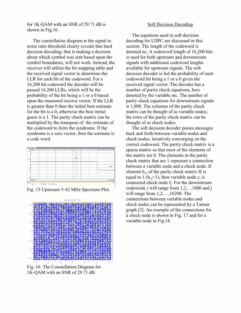
for 1K-QAM with an SNR of 29.71 dB is shown in Fig.16. The constellation diagram at the signal to noise ratio threshold clearly reveals that hard decision decoding, that is making a decision about which symbol was sent based upon the symbol boundaries, will not work. Instead, the receiver will utilize the bit mapping table and the received signal vector to determine the LLR for each bit of the codeword. For a 16,200 bit codeword the decoder will be passed 16,200 LLRs, which will be the probability of the bit being a 1 or a 0 based upon the measured receive vector. If the LLR is greater than 0 then the initial best estimate for the bit is a 0, otherwise the best initial guess is a 1. The parity check matrix can be multiplied by the transpose of the estimate of the codeword to form the syndrome. If the syndrome is a zero vector, then the estimate is a code word.

Fig. 15 Upstream 5-42 MHz Spectrum Plot.

Fig. 16. The Constellation Diagram for 1K-QAM with an SNR of 29.71 dB.

Soft Decision Decoding The equations used in soft decision decoding for LDPC are discussed in this section. The length of the codeword is denoted nc. A codeword length of 16,200 bits is used for both upstream and downstream signals with additional codeword lengths available for upstream signals. The soft decision decoder is fed the probability of each codeword bit being a 1 or a 0 given the received signal vector. The decoder has a number of parity check equations, here denoted by the variable mc. The number of parity check equations for downstream signals is 1,800. The columns of the parity check matrix can be thought of as variable nodes; the rows of the parity check matrix can be thought of as check nodes. The soft decision decoder passes messages back and forth between variable nodes and check nodes, iteratively converging on the correct codeword. The parity check matrix is a sparse matrix so that most of the elements of the matrix are 0. The elements in the parity check matrix that are 1 represent a connection between a variable node and a check node. If element hi,j of the parity check matrix H is equal to 1 (hi,j=1), then variable node ci is connected check node fj. For the downstream codeword, i will range from 1,2,…1800 and j will range from 1,2,…,16200. The connections between variable nodes and check nodes can be represented by a Tanner graph [2]. An example of the connections for a check node is shown in Fig. 17 and for a variable node in Fig.18.

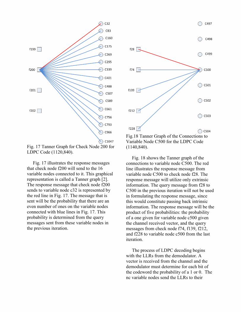
Fig. 17 Tanner Graph for Check Node 200 for LDPC Code (1120,840). Fig. 17 illustrates the response messages that check node f200 will send to the 16 variable nodes connected to it. This graphical representation is called a Tanner graph [2]. The response message that check node f200 sends to variable node c32 is represented by the red line in Fig. 17. The message that is sent will be the probability that there are an even number of ones on the variable nodes connected with blue lines in Fig. 17. This probability is determined from the query messages sent from these variable nodes in the previous iteration.

Fig.18 Tanner Graph of the Connections to Variable Node C500 for the LDPC Code (1140,840). Fig. 18 shows the Tanner graph of the connections to variable node C500. The red line illustrates the response message from variable node C500 to check node f28. The response message will utilize only extrinsic information. The query message from f28 to C500 in the previous iteration will not be used in formulating the response message, since this would constitute passing back intrinsic information. The response message will be the product of five probabilities: the probability of a one given for variable node c500 given the channel received vector, and the query messages from check node f74, f139, f212, and f228 to variable node c500 from the last iteration. The process of LDPC decoding begins with the LLRs from the demodulator. A vector is received from the channel and the demodulator must determine for each bit of the codeword the probability of a 1 or 0. The nc variable nodes send the LLRs to their

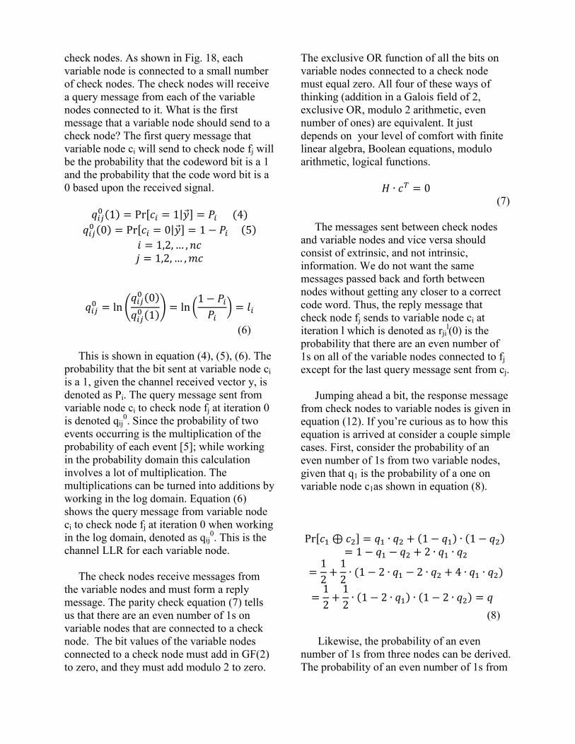
check nodes. As shown in Fig. 18, each variable node is connected to a small number of check nodes. The check nodes will receive a query message from each of the variable nodes connected to it. What is the first message that a variable node should send to a check node? The first query message that variable node ci will send to check node fj will be the probability that the codeword bit is a 1 and the probability that the code word bit is a 0 based upon the received signal.

(6) This is shown in equation (4), (5), (6). The probability that the bit sent at variable node ci is a 1, given the channel received vector y, is denoted as Pi. The query message sent from variable node ci to check node fj at iteration 0 is denoted qij

0. Since the probability of two events occurring is the multiplication of the probability of each event [5]; while working in the probability domain this calculation involves a lot of multiplication. The multiplications can be turned into additions by working in the log domain. Equation (6) shows the query message from variable node ci to check node fj at iteration 0 when working in the log domain, denoted as qij

0. This is the channel LLR for each variable node. The check nodes receive messages from the variable nodes and must form a reply message. The parity check equation (7) tells us that there are an even number of 1s on variable nodes that are connected to a check node. The bit values of the variable nodes connected to a check node must add in GF(2) to zero, and they must add modulo 2 to zero.

The exclusive OR function of all the bits on variable nodes connected to a check node must equal zero. All four of these ways of thinking (addition in a Galois field of 2, exclusive OR, modulo 2 arithmetic, even number of ones) are equivalent. It just depends on your level of comfort with finite linear algebra, Boolean equations, modulo arithmetic, logical functions.

(7) The messages sent between check nodes and variable nodes and vice versa should consist of extrinsic, and not intrinsic, information. We do not want the same messages passed back and forth between nodes without getting any closer to a correct code word. Thus, the reply message that check node fj sends to variable node ci at iteration l which is denoted as rji

l(0) is the probability that there are an even number of 1s on all of the variable nodes connected to fj except for the last query message sent from cj. Jumping ahead a bit, the response message from check nodes to variable nodes is given in equation (12). If you’re curious as to how this equation is arrived at consider a couple simple cases. First, consider the probability of an even number of 1s from two variable nodes, given that q1 is the probability of a one on variable node c1as shown in equation (8).

(8) Likewise, the probability of an even number of 1s from three nodes can be derived. The probability of an even number of 1s from

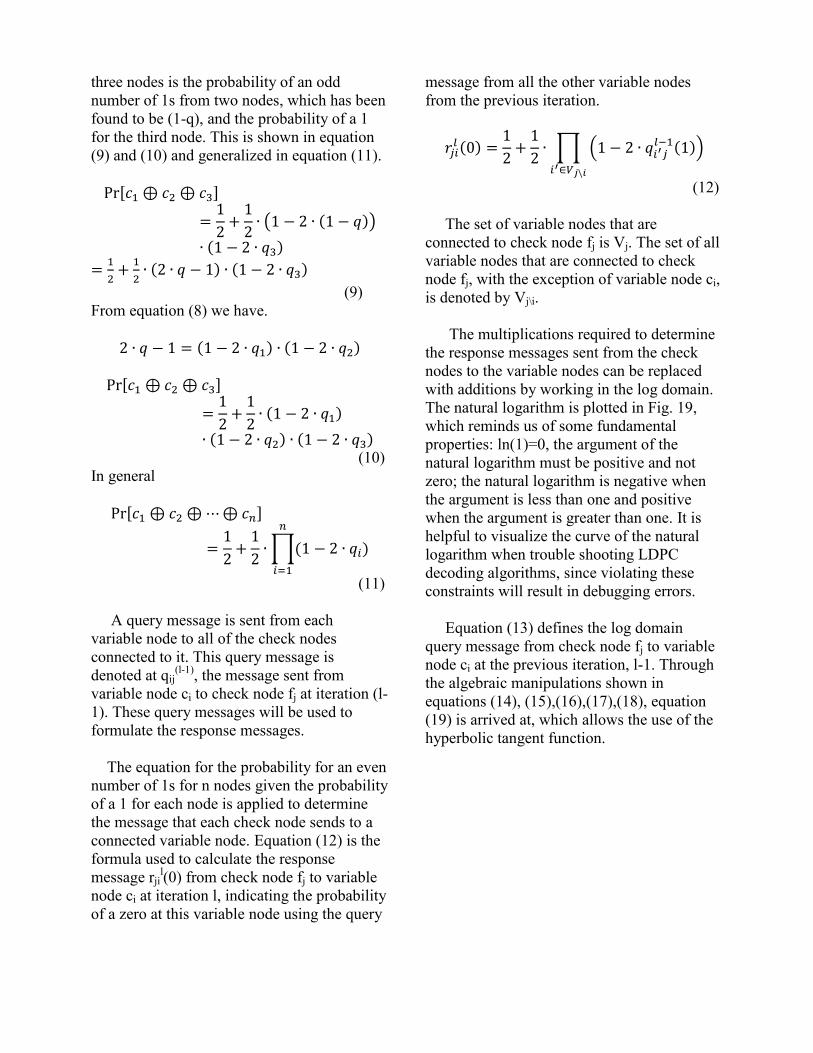
three nodes is the probability of an odd number of 1s from two nodes, which has been found to be (1-q), and the probability of a 1 for the third node. This is shown in equation (9) and (10) and generalized in equation (11).

(9) From equation (8) we have.

(10) In general

(11) A query message is sent from each variable node to all of the check nodes connected to it. This query message is denoted at qij

(l-1), the message sent from variable node ci to check node fj at iteration (l-1). These query messages will be used to formulate the response messages. The equation for the probability for an even number of 1s for n nodes given the probability of a 1 for each node is applied to determine the message that each check node sends to a connected variable node. Equation (12) is the formula used to calculate the response message rji

l(0) from check node fj to variable node ci at iteration l, indicating the probability of a zero at this variable node using the query

message from all the other variable nodes from the previous iteration.

(12) The set of variable nodes that are connected to check node fj is Vj. The set of all variable nodes that are connected to check node fj, with the exception of variable node ci, is denoted by Vj\i. The multiplications required to determine the response messages sent from the check nodes to the variable nodes can be replaced with additions by working in the log domain. The natural logarithm is plotted in Fig. 19, which reminds us of some fundamental properties: ln(1)=0, the argument of the natural logarithm must be positive and not zero; the natural logarithm is negative when the argument is less than one and positive when the argument is greater than one. It is helpful to visualize the curve of the natural logarithm when trouble shooting LDPC decoding algorithms, since violating these constraints will result in debugging errors. Equation (13) defines the log domain query message from check node fj to variable node ci at the previous iteration, l-1. Through the algebraic manipulations shown in equations (14), (15),(16),(17),(18), equation (19) is arrived at, which allows the use of the hyperbolic tangent function.

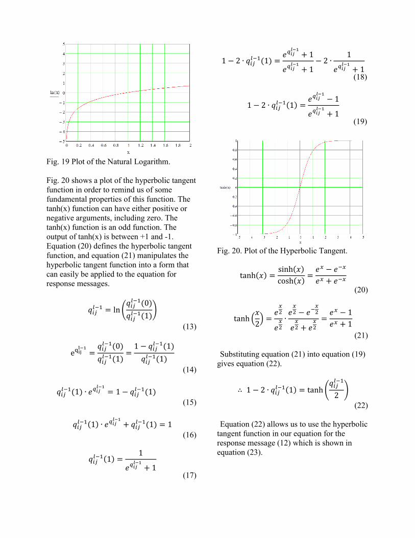
Fig. 19 Plot of the Natural Logarithm. Fig. 20 shows a plot of the hyperbolic tangent function in order to remind us of some fundamental properties of this function. The tanh(x) function can have either positive or negative arguments, including zero. The tanh(x) function is an odd function. The output of tanh(x) is between +1 and -1. Equation (20) defines the hyperbolic tangent function, and equation (21) manipulates the hyperbolic tangent function into a form that can easily be applied to the equation for response messages.

(13)

(14)

(15)

(16)

(17)

(18)

(19)

Fig. 20. Plot of the Hyperbolic Tangent.

(20)

(21) Substituting equation (21) into equation (19)

gives equation (22).

(22) Equation (22) allows us to use the hyperbolic

tangent function in our equation for the response message (12) which is shown in equation (23).

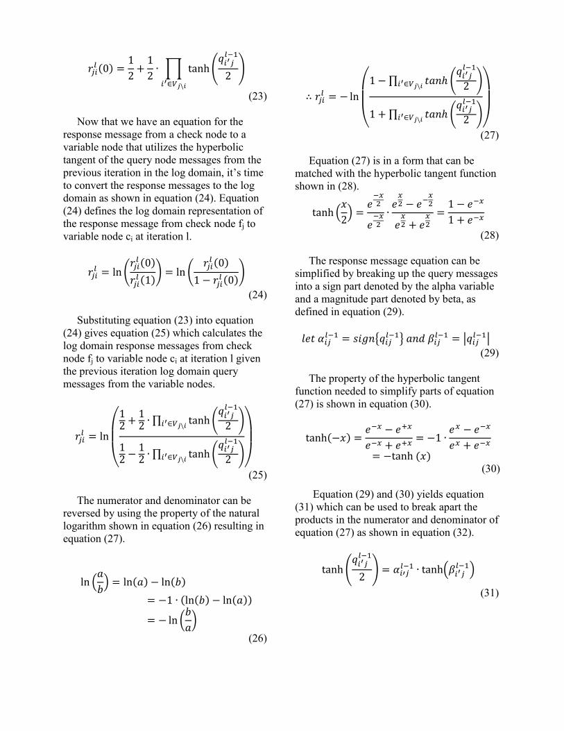
(23) Now that we have an equation for the response message from a check node to a variable node that utilizes the hyperbolic tangent of the query node messages from the previous iteration in the log domain, it’s time to convert the response messages to the log domain as shown in equation (24). Equation (24) defines the log domain representation of the response message from check node fj to variable node ci at iteration l.

(24) Substituting equation (23) into equation (24) gives equation (25) which calculates the log domain response messages from check node fj to variable node ci at iteration l given the previous iteration log domain query messages from the variable nodes.

(25) The numerator and denominator can be reversed by using the property of the natural logarithm shown in equation (26) resulting in equation (27).

(26)

(27) Equation (27) is in a form that can be matched with the hyperbolic tangent function shown in (28).

(28) The response message equation can be simplified by breaking up the query messages into a sign part denoted by the alpha variable and a magnitude part denoted by beta, as defined in equation (29).

(29) The property of the hyperbolic tangent function needed to simplify parts of equation (27) is shown in equation (30).

(30) Equation (29) and (30) yields equation

(31) which can be used to break apart the products in the numerator and denominator of equation (27) as shown in equation (32).

(31)

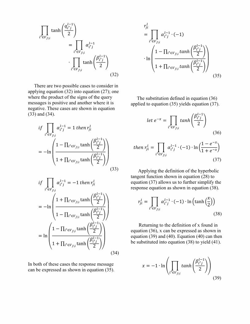
(32) There are two possible cases to consider in applying equation (32) into equation (27); one where the product of the signs of the query messages is positive and another where it is negative. These cases are shown in equation (33) and (34).

(33)

(34) In both of these cases the response message can be expressed as shown in equation (35).

(35) The substitution defined in equation (36) applied to equation (35) yields equation (37).

(36)

(37) Applying the definition of the hyperbolic tangent function shown in equation (28) to equation (37) allows us to further simplify the response equation as shown in equation (38).

(38) Returning to the definition of x found in

equation (36), x can be expressed as shown in equation (39) and (40). Equation (40) can then be substituted into equation (38) to yield (41).

(39)

(40)

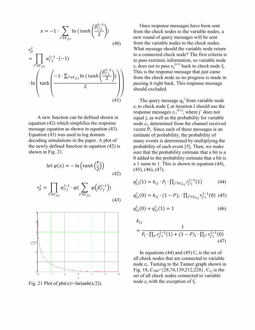
(41) A new function can be defined shown in equation (42) which simplifies the response message equation as shown in equation (43). Equation (43) was used in log domain decoding simulations in the paper. A plot of the newly defined function in equation (42) is shown in Fig. 21.

(42)

(43)

Fig. 21 Plot of phi(x)=-ln(tanh(x/2)).

Once response messages have been sent from the check nodes to the variable nodes, a new round of query messages will be sent from the variable nodes to the check nodes. What message should the variable node return to a connected check node? The first criteria is to pass extrinsic information, so variable node ci does not to pass rij

(l-1) back to check node fj. This is the response message that just came from the check node so no progress is made in passing it right back. This response message should excluded. The query message qij

l from variable node ci to check node fj at iteration l should use the response messages rj’i

(l-1), where j’ does not equal j, as well as the probability for variable node ci, determined from the channel received vector Pi. Since each of these messages is an estimate of probability, the probability of many events is determined by multiplying the probability of each event [5]. Then, we make sure that the probability estimate that a bit is a 0 added to the probability estimate that a bit is a 1 sums to 1. This is shown in equation (44), (45), (46), (47).

(44)

(45)

(46)

(47) In equations (44) and (45) Ci is the set of all check nodes that are connected to variable node ci. Turning to the Tanner graph shown in Fig. 18, C500={28,74,139,212,228}. Ci\j is the set of all check nodes connected to variable node ci with the exception of fj.

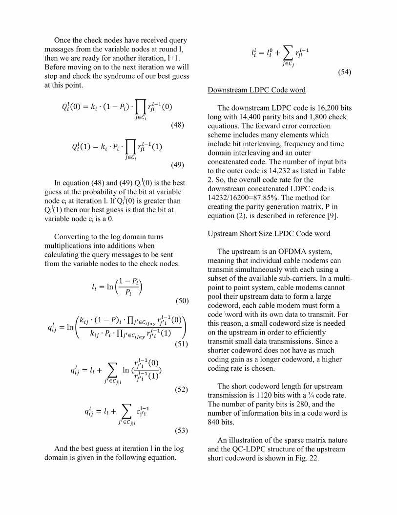
Once the check nodes have received query messages from the variable nodes at round l, then we are ready for another iteration, l+1. Before moving on to the next iteration we will stop and check the syndrome of our best guess at this point.

(48)

(49) In equation (48) and (49) Qi

l(0) is the best guess at the probability of the bit at variable node ci at iteration l. If Qi

l(0) is greater than Qi

l(1) then our best guess is that the bit at variable node ci is a 0. Converting to the log domain turns multiplications into additions when calculating the query messages to be sent from the variable nodes to the check nodes.

(50)

(51)

(52)

(53) And the best guess at iteration l in the log domain is given in the following equation.

(54) Downstream LDPC Code word The downstream LDPC code is 16,200 bits long with 14,400 parity bits and 1,800 check equations. The forward error correction scheme includes many elements which include bit interleaving, frequency and time domain interleaving and an outer concatenated code. The number of input bits to the outer code is 14,232 as listed in Table 2. So, the overall code rate for the downstream concatenated LDPC code is 14232/16200=87.85%. The method for creating the parity generation matrix, P in equation (2), is described in reference [9]. Upstream Short Size LPDC Code word The upstream is an OFDMA system, meaning that individual cable modems can transmit simultaneously with each using a subset of the available sub-carriers. In a multi-point to point system, cable modems cannot pool their upstream data to form a large codeword, each cable modem must form a code \word with its own data to transmit. For this reason, a small codeword size is needed on the upstream in order to efficiently transmit small data transmissions. Since a shorter codeword does not have as much coding gain as a longer codeword, a higher coding rate is chosen. The short codeword length for upstream transmission is 1120 bits with a ¾ code rate. The number of parity bits is 280, and the number of information bits in a code word is 840 bits. An illustration of the sparse matrix nature and the QC-LDPC structure of the upstream short codeword is shown in Fig. 22.

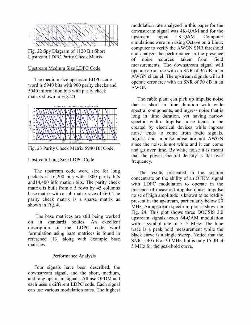
Fig. 22 Spy Diagram of 1120 Bit Short Upstream LDPC Parity Check Matrix. Upstream Medium Size LDPC Code The medium size upstream LDPC code word is 5940 bits with 900 parity checks and 5040 information bits with parity check matrix shown in Fig. 23.

Fig. 23 Parity Check Matrix 5940 Bit Code. Upstream Long Size LDPC Code The upstream code word size for long packets is 16,200 bits with 1800 parity bits and14,400 information bits. The parity check matrix is built from a 5 rows by 45 columns base matrix with a sub-matrix size of 360. The parity check matrix is a sparse matrix as shown in Fig. 4. The base matrices are still being worked on in standards bodies. An excellent description of the LDPC code word formulation using base matrices is found in reference [13] along with example base matrices.

Performance Analysis Four signals have been described; the downstream signal, and the short, medium, and long upstream signals. All use OFDM and each uses a different LDPC code. Each signal can use various modulation rates. The highest

modulation rate analyzed in this paper for the downstream signal was 4K-QAM and for the upstream signal 1K-QAM. Computer simulations were run using Octave on a Linux computer to verify the AWGN SNR threshold and analyze the performance in the presence of noise sources taken from field measurements. The downstream signal will operate error free with an SNR of 36 dB in an AWGN channel. The upstream signals will all operate error free with an SNR of 30 dB in an AWGN. The cable plant can pick up impulse noise that is short in time duration with wide spectral components, and ingress noise that is long in time duration, yet having narrow spectral width. Impulse noise tends to be created by electrical devices while ingress noise tends to come from radio signals. Ingress and impulse noise are not AWGN since the noise is not white and it can come and go over time. By white noise it is meant that the power spectral density is flat over frequency. The results presented in this section concentrate on the ability of an OFDM signal with LDPC modulation to operate in the presence of measured impulse noise. Impulse noise of high amplitude is known to be readily present in the upstream, particularly below 20 MHz. An upstream spectrum plot is shown in Fig. 24. This plot shows three DOCSIS 3.0 upstream signals, each 64-QAM modulation with a symbol rate of 5.12 MHz. The blue trace is a peak hold measurement while the black curve is a single sweep. Notice that the SNR is 40 dB at 30 MHz, but is only 15 dB at 5 MHz for the peak hold curve.

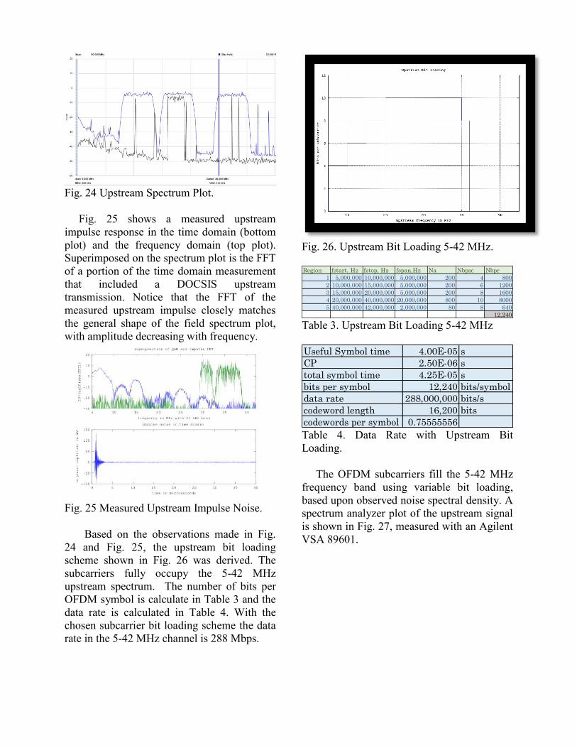
Fig. 24 Upstream Spectrum Plot. Fig. 25 shows a measured upstream impulse response in the time domain (bottom plot) and the frequency domain (top plot). Superimposed on the spectrum plot is the FFT of a portion of the time domain measurement that included a DOCSIS upstream transmission. Notice that the FFT of the measured upstream impulse closely matches the general shape of the field spectrum plot, with amplitude decreasing with frequency.

Fig. 25 Measured Upstream Impulse Noise. Based on the observations made in Fig. 24 and Fig. 25, the upstream bit loading scheme shown in Fig. 26 was derived. The subcarriers fully occupy the 5-42 MHz upstream spectrum. The number of bits per OFDM symbol is calculate in Table 3 and the data rate is calculated in Table 4. With the chosen subcarrier bit loading scheme the data rate in the 5-42 MHz channel is 288 Mbps.

Fig. 26. Upstream Bit Loading 5-42 MHz.

Table 3. Upstream Bit Loading 5-42 MHz

Table 4. Data Rate with Upstream Bit Loading. The OFDM subcarriers fill the 5-42 MHz frequency band using variable bit loading, based upon observed noise spectral density. A spectrum analyzer plot of the upstream signal is shown in Fig. 27, measured with an Agilent VSA 89601.

Region fstart, Hz fstop, Hz fspan,Hz Na Nbpsc Nbpr

1 5,000,000 10,000,000 5,000,000 200 4 800

2 10,000,000 15,000,000 5,000,000 200 6 1200

3 15,000,000 20,000,000 5,000,000 200 8 1600

4 20,000,000 40,000,000 20,000,000 800 10 8000

5 40,000,000 42,000,000 2,000,000 80 8 640

12,240

Useful Symbol time 4.00E-05 s

CP 2.50E-06 s

total symbol time 4.25E-05 s

bits per symbol 12,240 bits/symbol

data rate 288,000,000 bits/s

codeword length 16,200 bits

codewords per symbol 0.75555556

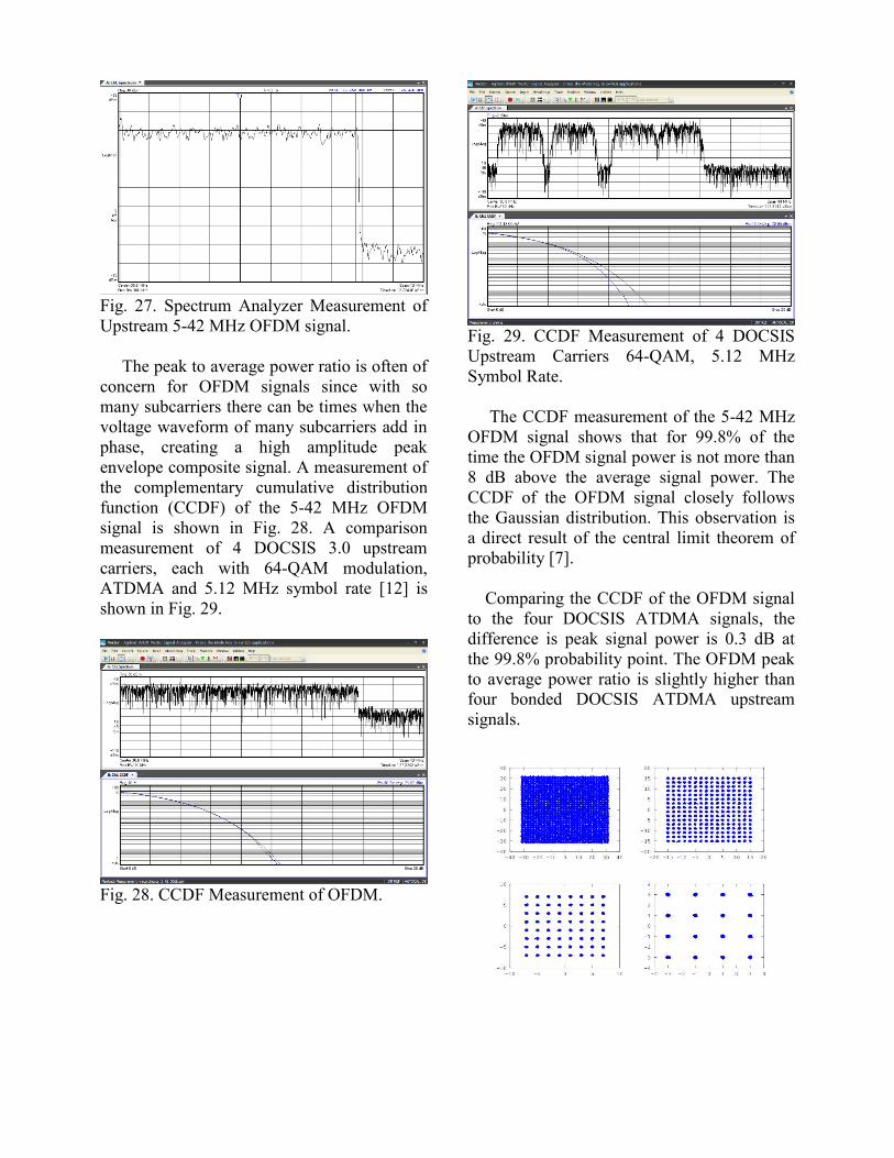
Fig. 27. Spectrum Analyzer Measurement of Upstream 5-42 MHz OFDM signal. The peak to average power ratio is often of concern for OFDM signals since with so many subcarriers there can be times when the voltage waveform of many subcarriers add in phase, creating a high amplitude peak envelope composite signal. A measurement of the complementary cumulative distribution function (CCDF) of the 5-42 MHz OFDM signal is shown in Fig. 28. A comparison measurement of 4 DOCSIS 3.0 upstream carriers, each with 64-QAM modulation, ATDMA and 5.12 MHz symbol rate [12] is shown in Fig. 29.

Fig. 28. CCDF Measurement of OFDM.

Fig. 29. CCDF Measurement of 4 DOCSIS Upstream Carriers 64-QAM, 5.12 MHz Symbol Rate. The CCDF measurement of the 5-42 MHz OFDM signal shows that for 99.8% of the time the OFDM signal power is not more than 8 dB above the average signal power. The CCDF of the OFDM signal closely follows the Gaussian distribution. This observation is a direct result of the central limit theorem of probability [7]. Comparing the CCDF of the OFDM signal to the four DOCSIS ATDMA signals, the difference is peak signal power is 0.3 dB at the 99.8% probability point. The OFDM peak to average power ratio is slightly higher than four bonded DOCSIS ATDMA upstream signals.

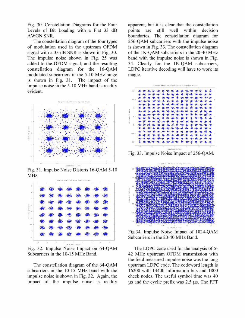
Fig. 30. Constellation Diagrams for the Four Levels of Bit Loading with a Flat 33 dB AWGN SNR. The constellation diagram of the four types of modulation used in the upstream OFDM signal with a 33 dB SNR is shown in Fig. 30. The impulse noise shown in Fig. 25 was added to the OFDM signal, and the resulting constellation diagram for the 16-QAM modulated subcarriers in the 5-10 MHz range is shown in Fig. 31. The impact of the impulse noise in the 5-10 MHz band is readily evident.

Fig. 31. Impulse Noise Distorts 16-QAM 5-10 MHz.

Fig. 32. Impulse Noise Impact on 64-QAM Subcarriers in the 10-15 MHz Band. The constellation diagram of the 64-QAM subcarriers in the 10-15 MHz band with the impulse noise is shown in Fig. 32. Again, the impact of the impulse noise is readily

apparent, but it is clear that the constellation points are still well within decision boundaries. The constellation diagram for 256-QAM subcarriers with the impulse noise is shown in Fig. 33. The constellation diagram of the 1K-QAM subcarriers in the 20-40 MHz band with the impulse noise is shown in Fig. 34. Clearly for the 1K-QAM subcarriers, LDPC iterative decoding will have to work its magic.

Fig. 33. Impulse Noise Impact of 256-QAM.

Fig.34. Impulse Noise Impact of 1024-QAM Subcarriers in the 20-40 MHz Band. The LDPC code used for the analysis of 5-42 MHz upstream OFDM transmission with the field measured impulse noise was the long upstream LDPC code. The codeword length is 16200 with 14400 information bits and 1800 check nodes. The useful symbol time was 40 μs and the cyclic prefix was 2.5 μs. The FFT

size was 2048 and the cyclix prefix was 128 time samples. The sampling frequency was 51.8 MHz. The center frequency of the IFFT output was chosen to be at 30.6 MHz so that the lowest frequency FFT subcarrier started at 5 MHz. The decoder used equations (43), (53), and (54), which is a standard flooding sum product message passing algorithm in the log domain. The general method used in the analysis was to first create 34 codewords, each 16200 bits, using the parity generation matrix. The complex symbols were created by dividing up the codeword bits to match the subcarrier bit loading and mapping bits to symbols for each modulation scheme and normalizing. Then, a signal could be generated by assigning complex symbols to OFDM subcarriers and applying an IFFT to create the time domain waveform. Then, the cyclic prefix could be added along with AWGN noise and delay echo. The field measured impulse noise was added to the time domain OFDM signal. The amplitude of the impulse was adjusted to match the power spectral density relationship between the field impulse measurement and the DOCSIS carriers. The impulse time domain signal was multiplied by the complex exponential of the center frequency difference in the field measurement and the simulation signal. This aligned the two signals in the freuqency domain. The impulse was adjusted so that the peak of the impulse fell in the midddle of the useful symbol time. The impulse was repeated for every OFDM symbol. In some cases the impulse repeats at a slow enough rate to allow for a time interleaver to correct for the errors due to the impulse. However, in this analysis the impulse repeats every symbol so that a time interleaver would not help. Then, the log-likelihood ratios for each of the codeword bits were determined. Finally,

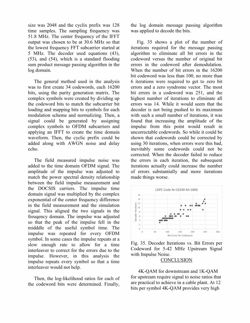
the log domain message passing algorithm was applied to decode the bits. Fig. 35 shows a plot of the number of iterations required for the message passing algorithm to eliminate all bit errors in the codeword versus the number of original bit errors in the codeword after demodulation. When the number of bit errors in the 16200 bit codeword was less than 100, no more than 6 iterations were required to get to zero bit errors and a zero syndrome vector. The most bit errors in a codeword was 251, and the highest number of iterations to eliminate all errors was 14. While it would seem that the decoder is not being pushed to its maximum with such a small number of iterations, it was found that increasing the amplitude of the impulse from this point would result in uncorrectable codewords. So while it could be shown that codewords could be corrected by using 30 iterations, when errors were this bad, inevitably some codewords could not be corrected. When the decoder failed to reduce the errors in each iteration, the subsequent iterations actually could increase the number of errors substantially and more iterations made things worse.

Fig. 35. Decoder Iterations vs. Bit Errors per Codeword for 5-42 MHz Upstream Signal with Impulse Noise.

CONCLUSION 4K-QAM for downstream and 1K-QAM for upstream require signal to noise ratios that are practical to achieve in a cable plant. At 12 bits per symbol 4K-QAM provides very high

0

2

4

6

8

10

12

14

16

0 50 100 150 200 250 300

Dec

od

er It

erat

ion

s

Bit Errors Per Codeword

LDPC Code N=16200 M=1800

spectral density, the number of bits per second that we can get out of a Hz of spectrum. Even at high spectral efficiency, Gbps data rates require wide channel widths. 192 MHz of channel width is required to get 1.87 Gbps of data rate using the downstream 4K-QAM and forward error correction. OFDM is very helpful in making such a wide channel width simple and practical. The FFT algorithm used to create 8,192 subcarriers is computationally very efficient. Using a 204.8 MHz sampling rate and an 8,192 point FFT, the channel is divided into subcarriers that are spaced apart in frequency by 25 kHz. The useful symbol time is 40 μs, which allows for a cyclic prefix of 2.5 μs to be added without sacrificing too much spectral efficiency. As long as reflections in the cable plant have a time delay less than the cyclic prefix they will not contribute to intersymbol interference. OFDM offers a simple mechanism to eliminate intersymbol interference due to reflections. The long symbol time and narrowband subcarriers can average out impulse noise while narrowband ingress noise only impacts a small number of subcarriers. Finally, LDPC codes have been shown to work well in AWGN channels and also to work well with impulse and ingress noise. The key principals of LDPC coding are using a large parity check matrix that is sparse, thus keeping the computational complexity manageable and still using a large enough sample of bits to have statistically significant information from the channel demodulator. The message passing decoder receives the LLRs for each bit of the codeword. Then, messages representing the probability of each bit are passed from variable nodes to check nodes and back until the codeword is found. Analysis was done by adding field measurements of noise to the OFDM signals. In many cases, such as in the example presented, the LDPC decoder could easily correct for the errors resulting from the

impulse noise. Many field measurements were analyzed in addition to the impulse shown in the example. The example impulse shown is very typical and almost all impulses observed had similar characteristics. The main factor in determining whether or not the decoder could correct all bit errors was the amplitude and frequency response of the impulse noise. At some point as the amplitude of the impulse was increased the decoder failed to correct bit errors. Once the decoder fails to keep reducing errors on every iteration, then the errors start to increase and additional iterations just make it worse. In the example shown, the amplitude of the impulse was adjusted to the highest possible for bit error free decoding. In most cases the amplitude and frequency response of the field measured impulse noise could easily be corrected by the LDPC decoder using the chosen bit loading scheme. However, this was not the case for all field measurements. In cases where the amplitude of the impulse noise or the frequency response of the impulse noise results in unacceptable bit errors, then there are still a number of remedies. One is time interleaving, which can help for a single impulse that does not repeat many times throughout the time interleaving process. Another remedy is to adjust the bit loading, reducing the bit loading to subcarriers most impacted by the impulse. Still, in general, it has been shown that high modulation rates such as 4K-QAM and 1K-QAM with OFDM and LDPC work well in the presence of field measured noise. Data rates of 1.87 Gbps in a 192 MHz downstream channel width and 288 Mbps in the upstream 5-42 MHz are possible using these techniques.

REFERENCES [1] R. Gallager, “Low density parity-check codes,” IRE Transactions on Information Theory, January 1962. [2] R.M. Tanner, “A Recursive Approach to Low Complexity Codes,” IEEE Transactions

on Information Theory, Vol. IT-27, NO. 5, September 1981. [3] Tuan Ta, “A Tutorial on Low Density Parity-Check Codes”, The University of Texas at Austin. [4] T.J. Richardson, R. Urbanke, D. Forney, S.Y. Chung, “On the Design of Low-Density Parity-Check Codes within 0.0045 dB of the Shannon Limit”, IEEE Communications Letters, Vol. 5, NO. 2, February 2001. [5] Athanasios Papoulis, “Probability, Random Variables, and Stochastic Processes”, McGraw-Hill, 1984, pp. 11, equation (1-8). [6] Tom Richardson, Rudiger Urbanke, “Modern Coding Theory”, Cambridge University Press, 2009. [7] Proakis J.G., Digital Communications, 2nd ed, McGraw-Hill, ISBN: 0-07-050937-9, 1989. [8] http://www.tvhistory.tv/1930-ATT-BELL-pg26-27.JPG

[9] Digital Video Broadcasting (DVB); Frame structure channel coding and modulation for a second generation digital transmission system for cable systems (DVB-C2), Draft ETSI EN 302 769 V1.0.2, 2009 [10] MacKay, D.J., Neal, R. M.: Near Shannon limit performance of low density parity check codes, Electronics Lett., Mar. 1997, vol. 33, no.6, pp. 457-458 [11] Research for Development of Future Interactive Generations of Hybrid Fiber Coax Networks (ReDeSign), www.ict-redesign.eu [12] Data Over Cable Service Interface Specifications, DOCSIS3.0, Physical Layer Specification, CM-SP-PHYv3.0-I08-090121, Cable Labs, January, 21, 2009. [13] Prodan, R. , Shen, B.Z., Lee, T. “DOWNSTREAM FEC PROPOSAL FOR IEEE 802.3 EPOC”, 3/11/2013 http://www.ieee802.org/3/bn/public/ma

r13/prodan_3bn_01_0313.pdf