Embed Size (px)
Citation preview

X-FAB Semiconductor Foundries Haarbergstraße 67 99097 Erfurt Germany phone +49 361 427 6663 fax +49 361 427 6631
Application Note SPICE Models & Simulations
Release 1.3 March 2014
Company Confidential ! Do not print or copy this document without permission of X-FAB Semiconductor Foundries!
SPICE Models & Simulations
Contents
INTRODUCTION ........................................................................................................................................... 1
1 MODELS ................................................................................................................................................ 1
1.1 CORNER MODELS ............................................................................................................................... 3
Predefined Parameter Sets (Corners) ............................................................................................. 3
Skewed Parameters ......................................................................................................................... 3
Disadvantages of corner model simulation ...................................................................................... 3
1.2 MONTE CARLO MODELS ..................................................................................................................... 4
Simulation Principle.......................................................................................................................... 4
Skewed Parameters ......................................................................................................................... 4
Modes of MC Simulation .................................................................................................................. 5
1.2.1 Process Variation ................................................................................................................... 5
1.2.2 Matching ................................................................................................................................. 7
1.2.3 both (Process Variation + Matching) ...................................................................................... 8
1.3 OPERATING CONDITION CHECK (OCC) MODELS .................................................................................. 9
1.4 LOT SPECIFIC MODELS (LSM) .......................................................................................................... 10
1.5 PRE-LAYOUT MODELS WITH PARASISTIC DIODES/CAPACITORS (PLPAR) ............................................ 11
2 SIMULATION SETUP .......................................................................................................................... 12
2.1 CADENCE 5.1 (SPECTRE) ................................................................................................................. 12
2.1.1 Corner Simulation ................................................................................................................. 12
2.1.2 Corner Simulation with the X-FAB Spectre Corner File Pre-Processor ............................... 14
2.1.3 Monte Carlo Simulation ........................................................................................................ 19
2.1.4 Operating Condition Check (OCC) ....................................................................................... 22
2.1.5 Lot Specific Models (LSM) ................................................................................................... 23
2.1.6 Pre-Layout Models With Parasistic Diodes/Capacitors (PLPar) .......................................... 24
2.2 CADENCE 6.1 (SPECTRE) ................................................................................................................. 25
2.2.1 Corner Simulation ................................................................................................................. 25
2.2.2 Corner Simulation with the X-FAB Spectre Corner File Pre-Processor ............................... 27
2.2.3 Monte Carlo Simulation ........................................................................................................ 28
2.2.4 Operating Condition Check (OCC) ....................................................................................... 31
2.2.5 Lot Specific Models (LSM) ................................................................................................... 31
2.2.6 Pre-Layout Models With Parasistic Diodes/Capacitors (PLPar) .......................................... 31
2.3 SYNOPSIS (HSPICE - NETLIST) .......................................................................................................... 32
2.3.1 Corner Simulation ................................................................................................................. 32
2.3.2 Monte Carlo Simulation ........................................................................................................ 33
2.3.3 Operating Condition Check (OCC) ....................................................................................... 34
2.3.4 Lot Specific Models (LSM) ................................................................................................... 35
2.3.5 Pre-Layout Models With Parasistic Diodes/Capacitors (PLPar) .......................................... 35
2.4 MENTOR (ELDO) ............................................................................................................................... 36
2.4.1 Corner Simulation ................................................................................................................. 36
2.4.2 Monte Carlo Simulation ........................................................................................................ 38
2.4.3 Operating Condition Check (OCC) ....................................................................................... 40
2.4.4 Lot Specific Models (LSM) ................................................................................................... 41
2.4.5 Pre-Layout Models With Parasistic Diodes/Capacitors (PLPar) .......................................... 41
2.5 PSPICE ............................................................................................................................................ 42
2.5.1 Corner Simulation ................................................................................................................. 42
2.5.2 Pre-Layout Models With Parasistic Diodes/Capacitors (PLPar) .......................................... 43
APPENDIX .................................................................................................................................................. 44

SPICE Models & Simulations
Figures Figure 1-1 principle of Process Variation (example: sheet resistance of rdn) .............................................. 6 Figure 1-2 principle of Matching (example: sheet resistance of rdn) ............................................................ 7 Figure 1-3 principle of Process Variation with Matching (example: sheet resistance of rdn) ....................... 8
Tables Table 1-1 SPICE model availability against process families and simulators .............................................. 2 Table 1-2 parameter mix in predefined X-FAB corners ................................................................................ 3 Table 1-3 example of an occ.err file .............................................................................................................. 9

SPICE Models & Simulations
Release 1.3 March 2014
Page 1 of 44 Company Confidential
Introduction X-FAB supports design kits for all major Electronic Design Automation (EDA) suppliers (Cadence, Mentor, Synopsis and Tanner) and their simulators (Spectre, Eldo, HSpice, PSpice and T-Spice) and offers accurate models that feature different analysis methods to enable robust and high-yielding designs. These SPICE simulation models shorten the development times. This document describes the possibilities and limitations of SPICE simulations and gives short introductions on how to prepare your EDA software (simulator).
1 Models X-FAB provides several types of SPICE/VerilogA models - the Corner Models, Monte Carlo Models (MC), Operating Condition Check Models (OCC), Lot Specific Models (LSM) and Pre-Layout-Parasitic Models (PLPar). They all help to optimize the design flow in different aspects and to evaluate the IC performance depending on the process parameter variations. Table 1-1 shows the featured SPICE models and their availability against the various X-FAB process families and supported simulators.

SPICE Models & Simulations
Release 1.3 March 2014
Page 2 of 44 Company Confidential
Process HSpice Eldo Spectre PSpice T-Spice
No
de
Fa
mily
Co
rne
r
MC
Pro
cess
MC
Ma
tch
ing
OC
C
LS
M
PL
Par
Co
rne
r
MC
Pro
cess
MC
Ma
tch
ing
OC
C
LS
M
PL
Par
Co
rne
r
MC
Pro
cess
MC
Ma
tch
ing
OC
C
LS
M
PL
Par
Co
rne
r
MC
Pro
cess
MC
Ma
tch
ing
OC
C
LS
M
PL
Par
Co
rne
r
MC
Pro
cess
MC
Ma
tch
ing
OC
C
LS
M
PL
Par
0.18µ XH018 var x - - var x - - var x - - - - - - - - HS HS HS HS - -
XC018 var x - - - var x - - - var x - - - - - - - - - HS HS HS - - -
XP018 var x - - var x - - var x - - - - - - - - HS HS HS - - -
XT018 var x - - var x - - var x - - - - - - - - HS HS HS HS - -
0.35µ XH035 var x x var x x var x x - - - - - - HS HS HS HS HS HS
XA035 var x x var x x var x x - - - - - - HS HS HS HS HS HS
XO035 var x - - var x - - var x - - - - - - - - HS HS - HS - -
XU035 var x - - var x - - var x - - - - - - - - HS HS HS HS - -
0.6µ CX06 fix - - - - - fix - - - - - fix - - - - - fix - - - - - HS - - - - -
XC06 fix x - x fix x - x fix x - x fix - - - - x HS HS HS HS - HS
XB06 fix x - - fix x - - fix x - - fix - - - - - HS HS HS HS - -
XT06 fix - - - - x fix - - - - x fix - - - - x fix - - - - x HS - - - - HS
0.8µ CX08A fix - - - - fix - - - - fix - - - - fix - - - - - HS - - HS - -
CX08H fix - - - - fix - - - - fix - - - x fix - - - - - HS - - HS - -
CX08N fix - - - - fix - - - - fix - - - - fix - - - - - HS - - HS - -
1.0µ XC10 fix - - - - - fix - - - - - fix - - - - - fix - - - - - HS - - - - -
XI10 fix - - - - - fix - - - - - fix - - - - - - - - - - - HS - - - - -
XDH10 fix - - - - - fix - - - - - fix - - - - - fix - - - - - HS - - - - -
XDM10 fix - - - - - fix - - - - - fix - - - - - fix - - - - - HS - - - - -
Table 1-1 SPICE model availability against process families and simulators Legend: → available x → partially available - → not available HS → HSpice Models are provided as specified in the HSpice column, but not explicitly verified with T-Spice MC Process → Monte Carlo Models show Process variation MC Matching → Monte Carlo Models show Matching Corner → Corner Models fix → corner models with fixed worst case parameters var → corner models with variable adjustable sigma (2s…6s) for worst case parameters OCC → Operating Condition Check Models LSM → Lot Specific Models PLPar → Pre-Layout Parasitic Models
SPICE Models & Simulations
Release 1.3 March 2014
Page 3 of 44 Company Confidential
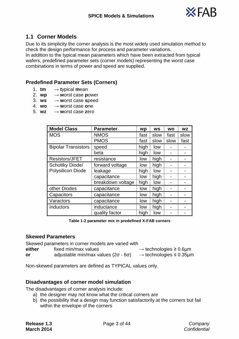
1.1 Corner Models
Due to its simplicity the corner analysis is the most widely used simulation method to check the design performance for process and parameter variations. In addition to the typical mean parameters which have been extracted from typical wafers, predefined parameter sets (corner models) representing the worst case combinations in terms of power and speed are supplied.
Predefined Parameter Sets (Corners)
1. tm → typical mean 2. wp → worst case power 3. ws → worst case speed 4. wo → worst case one 5. wz → worst case zero
Model Class Parameter wp ws wo wz
MOS NMOS fast slow fast slow
PMOS fast slow slow fast
Bipolar Transistors speed high low - -
beta high low - -
Resistors/JFET resistance low high - -
Schottky Diode/ Polysilicon Diode
forward voltage low high - -
leakage high low - -
capacitance low high - -
breakdown voltage high low - -
other Diodes capacitance low high - -
Capacitors capacitance low high - -
Varactors capacitance low high - -
Inductors inductance low high - -
quality factor high low - -
Table 1-2 parameter mix in predefined X-FAB corners
Skewed Parameters
Skewed parameters in corner models are varied with either fixed min/max values → technologies ≥ 0.6µm or adjustable min/max values (2σ - 6σ) → technologies ≤ 0.35µm Non-skewed parameters are defined as TYPICAL values only.
Disadvantages of corner model simulation
The disadvantages of corner analysis include: a) the designer may not know what the critical corners are b) the possibility that a design may function satisfactorily at the corners but fail
within the envelope of the corners

SPICE Models & Simulations
Release 1.3 March 2014
Page 4 of 44 Company Confidential
1.2 Monte Carlo Models
The Monte Carlo (MC) analysis is a series of DC, AC or TRANSIENT simulation runs, where a predefined sub-set of model parameters is varied by randomly simulator-generated values (skewed). These values range within the process parameter’s specific limits according to the selected distribution. In other words every single run of a Monte Carlo analysis is simulated with a new randomly generated corner.
Simulation Principle
assign randomly selected values to each
model parameter which should be varied
run the circuit simulation (.dc, .ac, .tran …)
Decide whether a new run has to be started.
The number of runs is defined by the
designer.
Complete MC simulation and display the
statistical results.
parameter
assignment
run SPICE
simulation
ready
begin
end
yes
no
Skewed Parameters
Skewed parameters in Monte Carlo models are varied randomly by the simulator (up to min/max value defined by the sigma input value) The skewed parameters are listed in two library files: .../simulator/technology/mc_params/mc_simulator_g.mod (.scs) .../simulator/technology/mc_params/mc_simulator_u.mod (.scs) Non-skewed parameters are defined as TYPICAL values only.

SPICE Models & Simulations
Release 1.3 March 2014
Page 5 of 44 Company Confidential
Modes of MC Simulation The designer can choose between two different types of parameter variation or use them in conjunction with each other. The principles of these variations will be described in the following sub-sections.
1.2.1 Process Variation
This Monte Carlo mode simulates the variation of the electrical parameters induced by unavoidable process fluctuations in manufacturing which effect all devices in a circuit in the same way. Therefore the process parameters, which are randomly selected in each simulation run are globally assigned to all device-instances in a design. Synonyms (several names which all mean the same):
lot variation
wafer variation
global variation
major variation Types of Process Parameter Distributions The MC analysis covers the whole parameter ranges which are defined by the statistical model set that is based on the worst case corner edge points. The probability of the values in the range, to be selected by the simulator, follow either a Gaussian or Uniform distribution. Choose between these two types in order to use their individual advantages in MC-simulations: Uniform:
artificial parameter distribution
only a few runs required to cover whole possible parameter range
potential to detect critical parameter combinations within the corner envelope
design centering: find device with the greatest influence on target parameter
Gaussian:
more realistic parameter distribution
a lot of simulation runs required to cover whole possible parameter range
yield estimation

SPICE Models & Simulations
Release 1.3 March 2014
Page 6 of 44 Company Confidential
Example: For every run, the simulator selects one value for the predefined Monte Carlo parameter RSH, which is the sheet resistance of the resistor rdn. The selection is based on the chosen distribution and is equally valid for every single instance of rdn in the design. Figure 1-1 illustrates the procedure that the simulator uses to randomly selects RSH only once in each run and assign it to every instance of rdn equally. In this example the value selection for run n is around -2σ and for run n+1 around +3σ. Gaussian distribution has been selected. As a result all the instances of rdn A, B and C are simulated with the same sheet resistance (blue points).
[RSH]=Ω/□
Pro
ce
ss
Va
ria
tio
nIn
sta
nc
e V
alu
e
tm-6σ
[RSHC]=Ω/□
[RSHB]=Ω/□
[RSHA]=Ω/□
gaussian
uniform
+6σrun n+1
device rdn
rdn-instances
run n
[RSH]=Ω/□
rdnn+1
rdnn
or
rdnn+1rdnn
A
B
C
Figure 1-1 principle of Process Variation (example: sheet resistance of rdn)
In the above explanation, the RSH variation is explained. In an actual simulation, all the other parameters are also varied at the same time using the same fundamental principles.
SPICE Models & Simulations
Release 1.3 March 2014
Page 7 of 44 Company Confidential
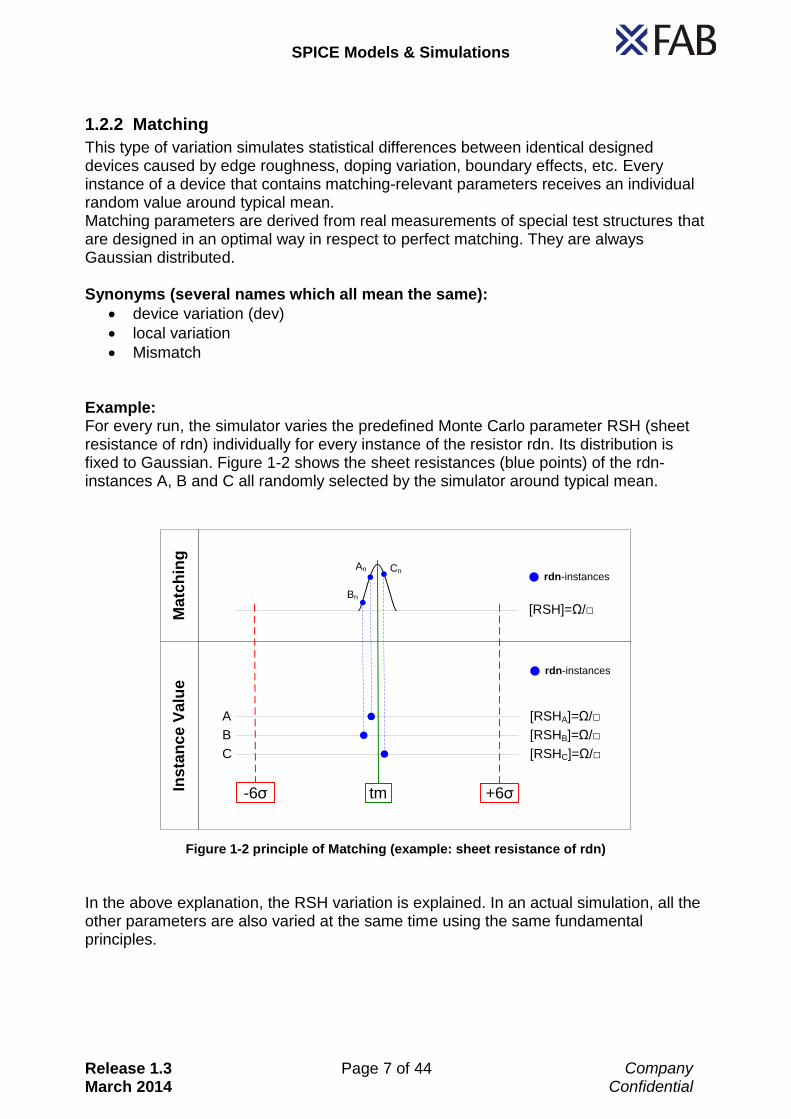
1.2.2 Matching
This type of variation simulates statistical differences between identical designed devices caused by edge roughness, doping variation, boundary effects, etc. Every instance of a device that contains matching-relevant parameters receives an individual random value around typical mean. Matching parameters are derived from real measurements of special test structures that are designed in an optimal way in respect to perfect matching. They are always Gaussian distributed. Synonyms (several names which all mean the same):
device variation (dev)
local variation
Mismatch Example: For every run, the simulator varies the predefined Monte Carlo parameter RSH (sheet resistance of rdn) individually for every instance of the resistor rdn. Its distribution is fixed to Gaussian. Figure 1-2 shows the sheet resistances (blue points) of the rdn-instances A, B and C all randomly selected by the simulator around typical mean.
Ma
tch
ing
Ins
tan
ce
Va
lue
tm +6σ-6σ
[RSHC]=Ω/□
[RSHB]=Ω/□
[RSHA]=Ω/□
[RSH]=Ω/□
rdn-instances
rdn-instances
An
Bn
Cn
A
B
C
Figure 1-2 principle of Matching (example: sheet resistance of rdn)
In the above explanation, the RSH variation is explained. In an actual simulation, all the other parameters are also varied at the same time using the same fundamental principles.

SPICE Models & Simulations
Release 1.3 March 2014
Page 8 of 44 Company Confidential
1.2.3 both (Process Variation + Matching)
Using both types of variation in conjunction with each other means that affected devices have a degree of independence (Mismatch), even though they share the same process variation (lot). Example: The interaction of Process Variation and Matching is shown in Figure 1-3. In one run the simulator first selects one value for RSH from its predefined process range dependent on the chosen distribution. In the second step the simulator varies the sheet resistance of each rdn-instance individually around the first selected Process value. In other words MC simulation with both variation types means that the sheet resistance of a rdn-instance is the addition of a global portion, which is shared by all instances in this run, and an individual portion.
[RSH]=Ω/□
Pro
ce
ss
Va
ria
tio
nM
atc
hin
gIn
sta
nc
e V
alu
e
tm-6σ
[RSHC]=Ω/□
[RSHB]=Ω/□
[RSHA]=Ω/□
gaussian
uniform
[RSH]=Ω/□
+6σrun n+1
rdn-instances
device rdn
rdn-instances
An
Bn
Cn
run n
[RSH]=Ω/□
An+1
Bn+1
Cn+1
rdnn+1
rdnn
or
rdnn+1rdnn
A
B
C
Figure 1-3 principle of Process Variation with Matching (example: sheet resistance of rdn)
The MC-simulation predictions are based upon a good layout in accordance to the guidelines in the Matching Manual.

SPICE Models & Simulations
Release 1.3 March 2014
Page 9 of 44 Company Confidential
1.3 Operating Condition Check (OCC) Models
The operating conditions, that are defined in the process specification document, denote the maximum ratings for all devices. To test your design for operating within the allowed conditions, invoke a transient simulation with special OCC libraries. During a simulation the conditions are inspected in intervals that are based upon a time step defined by the user in a section of the library tstep_occ.*. Occurrences of violations are written to the ASCII file “occ.err”. Check Table 1-1 for availability of the occ libraries in your preferred technology.
Device Parameter OC-Event Limit Time Instance
cpoly Vpm leaving OCA (>5.5V) at 0.000000e+00 I3.C0.occ_m1
pmos4 VDpsub leaving OCA (>5.5V) at 0.000000e+00 I2.M18.occ_m1
pghv VDB leaving OCA (>0.5V) at 1.590018e-06 I3.M3.occ_m1
cpoly Vpm entering OCA (-5.5V..5.5V) at 3.679900e-06 I3.C0. occ_m1
nhv VSB leaving OCA (>11.0V) at 4.654617e-06 I3.M1.occ_m1
nhv VSB leaving OCA (>11.0V) at 4.654617e-06 I3.M2.occ_m1
pghv VDB entering OCA (-25.0V..0.5V) at 6.545138e-06 I3.M3.occ_m1
nhv VSB entering OCA (-0.5V..11.0V) at 2.006150e-03 I3.M1.occ_m1
nhv VSB entering OCA (-0.5V..11.0V) at 2.006150e-03 I3.M2.occ_m1
cpoly Vpm leaving OCA (>5.5V) at 2.009185e-03 I3.C0.occ_m1
pghv VDB leaving OCA (>0.5V) at 5.001485e-03 I3.M3.occ_m1
cpoly Vpm entering OCA (-5.5 V..5.5V) at 5.003387e-03 I3.C0.occ_m1
nhv VSB leaving OCA (>11.0V) at 5.004651e-03 I3.M1.occ_m1
nhv VSB leaving OCA (>11.0V) at 5.004651e-03 I3.M2.occ_m1
pghv VDB entering OCA (-25.0V..0.5V) at 5.006209e-03 I3.M3.occ_m1
Table 1-3 example of an occ.err file
the “occ.err” file indicates “leaving” and “entering” of the Operating Conditions Area (OCA)
the designer has the complete “responsibility” to evaluate and to interpret the existing events/violations
the “OCC” simulation method is only a terminal voltage monitor of primitive devices within a circuit
experiences show, that primitive devices of intermediate circuit nodes (eg. compensation capacitors or capacitive coupling) are more likely to violate operating conditions rather than devices which are directly connected to the power supply rails
X-FAB provides the platform-independent Java program Occ_Analyzer.jar (available on X-TIC) in order to assist the designer with organizing, filtering and visualizing the OCC results.

SPICE Models & Simulations
Release 1.3 March 2014
Page 10 of 44 Company Confidential
Lot Specific Models (LSM)
Wafer specific Spice models can be used to simulate a design with the actual primitive device parameters that are found on the wafer. A Spice model library altered specifically to the parametric values of a wafer offers the possibility to re-simulate a circuit with the actual characteristics found for the devices on the wafer. This should help with the identification of any parameter offsets observed between the original simulations and the test results. Specific Spice models are generated for single wafers of prototype lots. Only the 'tm' values of the parameters in the skew files are altered, not the models, thus the simulated device characteristics are close to the measured characteristics found on the wafer. The generation of models, more precisely the skew parameter values, is done through a correlation matrix processed with a generation program. The correlations are obtained by analyzing variances of the PCM values. The parameter files are available for download from an online report. Contact X-FAB’s ebusiness team at [email protected] to get access to the data. Prepare the LSM simulations by downloading the WSM file that contains an html logfile and the wafer specific parameter files for three different simulators (Spectre, HSpice and Eldo). Extract these files to a directory of your choice. The resulting path is
~directory/[LotID]_w[WaferNo.]/ e.g. the path for wafer no.3 of lot M15880 is: ~mydirectory/M15880_W03/ The parameters can be checked with 'logfile.html' before usage to verify that the devices in question got their parameters changed. Those parameters where PCM values are not available either due to the process module selection or reduced PCM data set remain unchanged and are marked with 'UNCHANGED'. All parameter have unique recognizable names for reference to the appropriate device. Very few minor devices not getting Monte Carlo modeling have not generated parameter either. For reference compare the Spice library. Check Table 1-1 for availability of LSM models in your preferred technology.

SPICE Models & Simulations
Release 1.3 March 2014
Page 11 of 44 Company Confidential
1.4 Pre-Layout Models With Parasistic Diodes/Capacitors (PLPar)
Devices hold unavoidable parasitic elements, which can have a dramatic influence on the intended electrical behaviour of the designed circuit. Special software tools are able to extract these parasitics from the layout, add them to the schematic and allow a post-layout simulation, which provides more realistic results. In the early phase of developing a circuit, a layout is not available for parasitic extraction. To get a rough idea of the influence of parasitic elements, the designer is able to simulate with special Pre-Layout models with Parasitic diodes/capacitors (PLPar), the critical devices have additional parasitic elements, which are estimated in a simplified way. It is important to use either the pre-layout variant with special PLPar model libraries, or the more realistic post-layout simulation with the help of parasitic extraction tools. Avoid using both, otherwise the parasitic elements will be included twice giving inaccurate and pessimistic simulations. Check Table 1-1 for availability of PLPar models in your preferred technology.

SPICE Models & Simulations
Release 1.3 March 2014
Page 12 of 44 Company Confidential
2 Simulation Setup
2.1 Cadence 5.1 (Spectre)
Start Cadence
type in c-shell (csh, tcsh): first time: tkit –tech technology –tool artist –m fb
next times: icfb&
2.1.1 Corner Simulation
1.
start the Analog Design Environment (ADE) from the Schematic Editing window Tools → Analog Environment
setup the usual simulation variables (analyses, outputs, etc.)
2. start Model Library Setup dialogue from the ADE window
Setup → Model Libraries …
include param.scs and specify the sigma (Section: 2s,3s,4s,5s,6s) → only for technologies ≤0.35µm
include Model Library File(s) (technology.scs or bip.scs, res.scs, etc.) and set a corner (Section: tm,wp,ws,wo,wz)
3. start simulation from the ADE window
Simulation → Netlist and Run …

SPICE Models & Simulations
Release 1.3 March 2014
Page 13 of 44 Company Confidential
Sigma: 2s...6s
}Corners:
tm,wp,ws,wo,wz
Netlist
and Run
1.
2.
3.

SPICE Models & Simulations
Release 1.3 March 2014
Page 14 of 44 Company Confidential
2.1.2 Corner Simulation with the X-FAB Spectre Corner File Pre-Processor
The X-FAB Spectre Corner File Generator is a pre-processor to give help to designers for setting up Corner Simulations. It is not a stand alone Corner Analysis Tool and only works in conjunction with the Cadence Corner Analysis Tool. The X-FAB Spectre Corner File Generator is just a script to generate a setup file that can be loaded into the Cadence Corner Analysis Tool to get started quickly. 1. Start the Analog Design Environment 1.1. Setup your Simulation Run completely
1.2 Choose “X-FAB Spectre Corner FILE” from the “Corner-Tools” Menu
1.3. the following form should appear:
name of your corner setup file that will be created
name of your supply voltage design variable
2.
1.2

SPICE Models & Simulations
Release 1.3 March 2014
Page 15 of 44 Company Confidential
2. Setup your Corner combinations
2.1. Setup your Corner combinations by selecting “Setup Single Corners” and then choosing the combinations by using the cyclic radio buttons
2.2 Add as many Corner Combinations as you like by selecting “Setup Single Corners”
2.3 Give your Corner combinations reasonable names as shown in the picture below
2.4. Press the “Apply” button to create the “CornerFile.dcf” file 2.5. If you do not change the default setup, you will get a file named “CornerFile.dcf” in your cadence working directory.
2.2
2.3
SPICE Models & Simulations
Release 1.3 March 2014
Page 16 of 44 Company Confidential
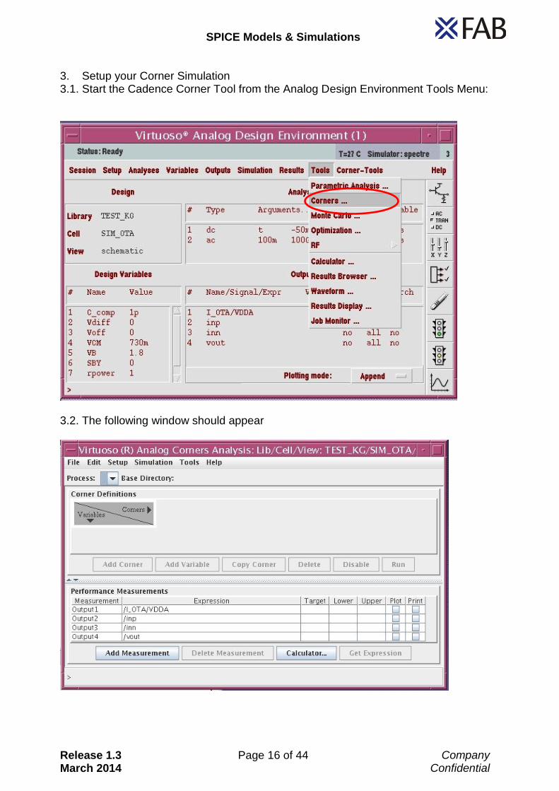
3. Setup your Corner Simulation 3.1. Start the Cadence Corner Tool from the Analog Design Environment Tools Menu:
3.2. The following window should appear
SPICE Models & Simulations
Release 1.3 March 2014
Page 17 of 44 Company Confidential
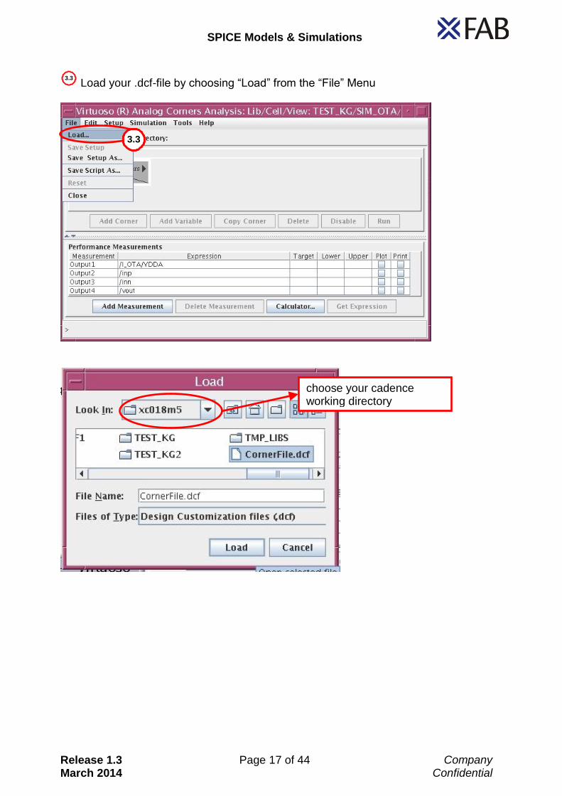
3.3 Load your .dcf-file by choosing “Load” from the “File” Menu
choose your cadence working directory
3.3

SPICE Models & Simulations
Release 1.3 March 2014
Page 18 of 44 Company Confidential
3.4. Your Cadence Corner Analysis Tool should now look like:
3.5. Press “Run” to run the Corner Simulation 3.6. For more information just have a look to the Cadence documentation.
3.5

SPICE Models & Simulations
Release 1.3 March 2014
Page 19 of 44 Company Confidential
2.1.3 Monte Carlo Simulation
1.
start the Analog Design Environment (ADE) from the Schematic Editing window Tools → Analog Environment
setup usual simulation variables (analyses, outputs, etc.)
2. start Model Library Setup dialogue from the ADE window
Setup → Model Libraries …
include param.scs and specify the sigma (Section: 2s,3s,4s,5s,6s)
include Model Library File (technology.scs, e.g. xh035.scs) and choose the distribution-type for process variation by setting the Section to:
mc_g → Gaussian mc_u → Uniform
if device-class-specific library files (bip.scs, bsim3v3.scs, etc.) are used, disable them to avoid double-defined models and parameters
3.
start Monte Carlo setup from the ADE window Tools → Monte Carlo …
set number of runs
choose type of parameter variation: Process Only, Mismatch Only or Process & Mismatch
more options to control the simulation specifically
4. start simulation from the Monte Carlo (Analog Statistical Analysis) window
Simulation → Run …

SPICE Models & Simulations
Release 1.3 March 2014
Page 20 of 44 Company Confidential
Gaussian: mc_g
Sigma: 2s...6s
Uniform: mc_u
1.
2.

SPICE Models & Simulations
Release 1.3 March 2014
Page 21 of 44 Company Confidential
Process Only
Mismatch Only
Process & Mismatch
Run ...
3.
4.

SPICE Models & Simulations
Release 1.3 March 2014
Page 22 of 44 Company Confidential
2.1.4 Operating Condition Check (OCC)
1. open Model Library Setup dialogue as shown in paragraph 2.1.1
2.
change model paths to occ models and add two more files: I. tstep_occ.scs
→ define time step of checking interval in the ‘Section’ area II. technology.occ (e.g. xh035.occ)
→ library with the VerilogA modules (Leave ‘Section’ blank!) The structure of the library-directories, where to find the occ models and the additional files depends on the used technology: ≥0.6µm: …/technologyocc/module/bsim3v3.scs
… …/technologyocc/module/technology.occ …/technologyocc/module/tstep_occ.lib
NO Section!
{
special
OCC files
special major
occ-directory
time step
≤0.35µm: …/technology/occ/module/bsim3v3.scs
… …/technology/occ/module/technology.occ
…/technology/occ/module/tstep_occ.lib
NO Section!
{
special
OCC files
inserted occ-directory
in library parth
time step
3. Start transient simulation from Analog Design Environment (ADE) window
SPICE Models & Simulations
Release 1.3 March 2014
Page 23 of 44 Company Confidential
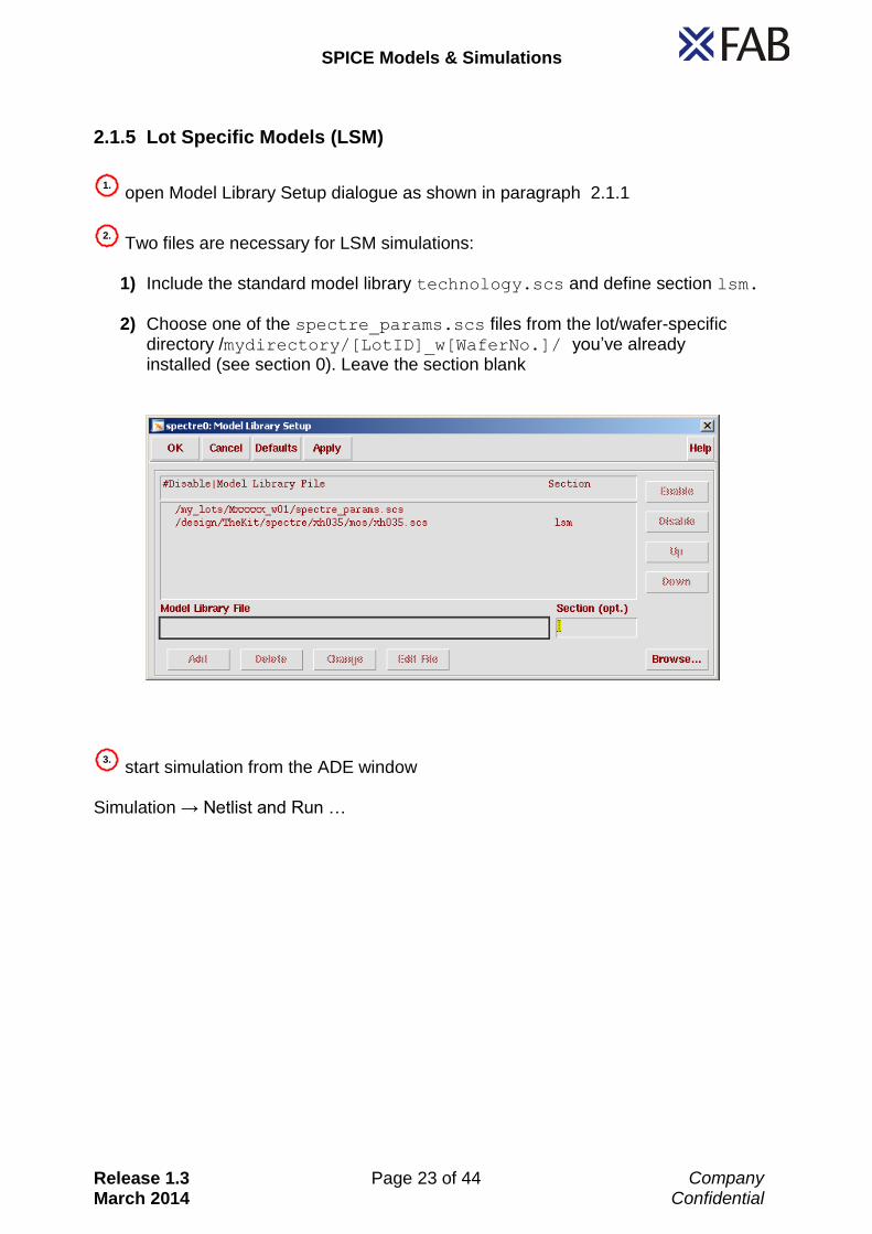
2.1.5 Lot Specific Models (LSM)
1.
open Model Library Setup dialogue as shown in paragraph 2.1.1
2. Two files are necessary for LSM simulations:
1) Include the standard model library technology.scs and define section lsm.
2) Choose one of the spectre_params.scs files from the lot/wafer-specific
directory /mydirectory/[LotID]_w[WaferNo.]/ you’ve already installed (see section 0). Leave the section blank
3. start simulation from the ADE window
Simulation → Netlist and Run …

SPICE Models & Simulations
Release 1.3 March 2014
Page 24 of 44 Company Confidential
2.1.6 Pre-Layout Models With Parasistic Diodes/Capacitors (PLPar)
1.
open Model Library Setup dialogue
include param.scs from the common directory as shown in section 2.1.1 and specify the sigma (Section: 2s,3s,4s,5s,6s) → only for technologies ≤0.35µm
choose one of the available Model Library File(s) (technology.scs or bsim3v3.scs, etc.) from the directory …/technology/spectre/module/parasitics/technology.scs and set a corner (Section: tm,wp,ws,wo,wz)
2. In some parasitic models, a global substrate node is used in addition to the
device nodes.
→ global node name: “psub!“
This global substrate node must be connected to the device substrate node.
3. start simulation from the ADE window
Simulation → Netlist and Run …

SPICE Models & Simulations
Release 1.3 March 2014
Page 25 of 44 Company Confidential
2.2 Cadence 6.1 (Spectre)
Start Cadence
type in c-shell (csh, tcsh): first time: tkit –tech technology
next times: virtuoso&
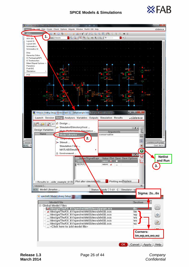
2.2.1 Corner Simulation
1.
start ADE L or higher from the Virtuoso Schematic Editor Launch → ADE L
setup the usual simulation variables (analyses, outputs, etc.)
2. start Model Library Setup dialogue from the ADE window
Setup → Model Libraries …
include param.scs and specify the sigma (Section: 2s,3s,4s,5s,6s) → only for technologies ≤0.35µm
include Model Library File(s) (technology.scs or bip.scs, res.scs, etc.) and set a corner (Section: tm,wp,ws,wo,wz)
3. start simulation from the ADE window
Simulation → Netlist and Run …
SPICE Models & Simulations
Release 1.3 March 2014
Page 26 of 44 Company Confidential
Sigma: 2s...6s
}Corners:
tm,wp,ws,wo,wz
Netlist
and Run
1.
2.
3.

SPICE Models & Simulations
Release 1.3 March 2014
Page 27 of 44 Company Confidential
2.2.2 Corner Simulation with the X-FAB Spectre Corner File Pre-Processor
In Cadence 6.1 the X-FAB Spectre Corner File Pre-Processor is not supported anymore.

SPICE Models & Simulations
Release 1.3 March 2014
Page 28 of 44 Company Confidential
2.2.3 Monte Carlo Simulation
1. Start the Analog Design Environment
1.1 start ADE XL or higher from the Virtuoso Schematic Editor
Launch → ADE XL
1.2
1.3 confirm appearing dialog boxes by pressing OK
1.4
add a new Test (ADE XL Test Editor is started)
setup usual simulation variables (analyses, outputs, etc.)
2. open Model Library Setup dialogue from the ADE XL Test Editor window
Setup → Model Libraries …
include param.scs and specify the sigma (Section: 2s,3s,4s,5s,6s)
include Model Library File (technology.scs, e.g. xh035.scs) and choose the distribution-type for process variation by setting the Section to:
mc_g → Gaussian mc_u → Uniform
if device-class-specific library files (bip.scs, bsim3v3.scs, etc.) are used, disable them to avoid double-defined models and parameters
3.
select the Run Mode Monte Carlo Sampling from the ADE window Tools → Monte Carlo …
set number of runs
choose type of parameter variation: Process Only, Mismatch Only or Process & Mismatch
more options to control the simulation specifically
4. setup Monte Carlo simulation
5.
start simulation

SPICE Models & Simulations
Release 1.3 March 2014
Page 29 of 44 Company Confidential
1.1
Gaussian: mc_g
Sigma: 2s...6s
Uniform: mc_u
2.
1.2
1.3
1.4

SPICE Models & Simulations
Release 1.3 March 2014
Page 30 of 44 Company Confidential
3.
5.4.
SPICE Models & Simulations
Release 1.3 March 2014
Page 31 of 44 Company Confidential
2.2.4 Operating Condition Check (OCC)
The specifics of OCC simulation in Cadence 6.1 is similar to Cadence 5.1 as shown in section 2.1.4.
2.2.5 Lot Specific Models (LSM)
The specifics of simulation with lot-specific models in Cadence 6.1 is similar to Cadence 5.1 as shown in section 2.1.5.
2.2.6 Pre-Layout Models With Parasistic Diodes/Capacitors (PLPar)
The specifics of simulation with pre-layout parasitics in Cadence 6.1 is similar to Cadence 5.1 as shown in section 2.1.6.
SPICE Models & Simulations
Release 1.3 March 2014
Page 32 of 44 Company Confidential
2.3 Synopsis (HSpice - Netlist)
In order to use the X-FAB Models in HSpice netlists, the following statements are required.
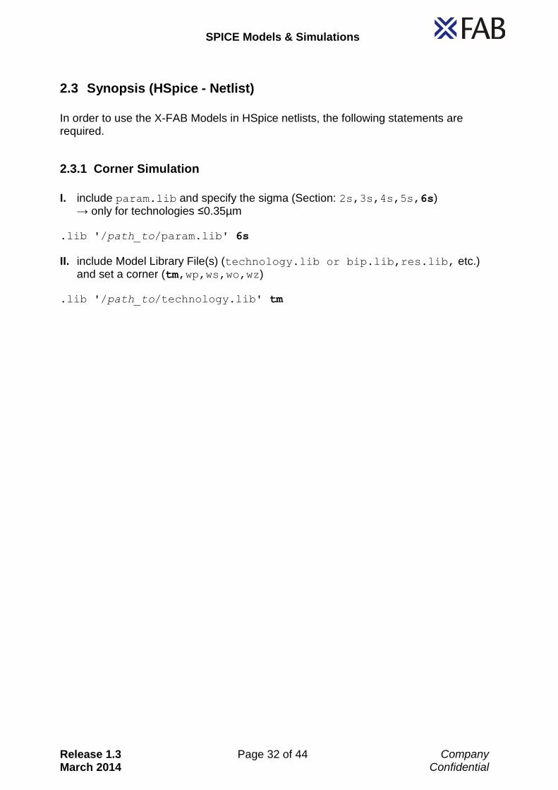
2.3.1 Corner Simulation
I. include param.lib and specify the sigma (Section: 2s,3s,4s,5s,6s)
→ only for technologies ≤0.35µm .lib '/path_to/param.lib' 6s
II. include Model Library File(s) (technology.lib or bip.lib,res.lib, etc.)
and set a corner (tm,wp,ws,wo,wz) .lib '/path_to/technology.lib' tm
SPICE Models & Simulations
Release 1.3 March 2014
Page 33 of 44 Company Confidential
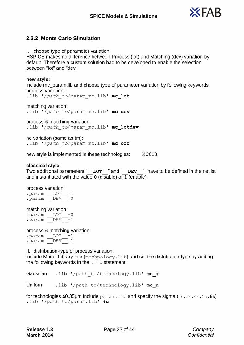
2.3.2 Monte Carlo Simulation
I. choose type of parameter variation HSPICE makes no difference between Process (lot) and Matching (dev) variation by default. Therefore a custom solution had to be developed to enable the selection between "lot" and "dev". new style: include mc_param.lib and choose type of parameter variation by following keywords: process variation: .lib '/path_to/param_mc.lib' mc_lot
matching variation: .lib '/path_to/param_mc.lib' mc_dev
process & matching variation: .lib '/path_to/param_mc.lib' mc_lotdev
no variation (same as tm): .lib '/path_to/param_mc.lib' mc_off
new style is implemented in these technologies: XC018 classical style: Two additional parameters “__LOT__” and “__DEV__” have to be defined in the netlist and instantiated with the value 0 (disable) or 1 (enable). process variation: .param __LOT__=1 .param __DEV__=0
matching variation: .param __LOT__=0 .param __DEV__=1
process & matching variation: .param __LOT__=1 .param __DEV__=1
II. distribution-type of process variation include Model Library File (technology.lib) and set the distribution-type by adding the following keywords in the .lib statement: Gaussian: .lib '/path_to/technology.lib' mc_g Uniform: .lib '/path_to/technology.lib' mc_u for technologies ≤0.35µm include param.lib and specify the sigma (2s,3s,4s,5s,6s) .lib '/path_to/param.lib' 6s

SPICE Models & Simulations
Release 1.3 March 2014
Page 34 of 44 Company Confidential
2.3.3 Operating Condition Check (OCC)
Prepare netlist by changing the model paths to occ models and add two more files I. tstep_occ.lib
→ define time step of checking interval as a section behind the .lib statement II. technology.occ (e.g. xh035.occ)
→ library with the VerilogA modules (Do not define a section!) The structure of the library-directories, where to find the occ models and the additional files depends on the used technology: You have to replace [simulator] by “eldo” or “hspice” because these statements apply to HSpice and Eldo as well! ≥0.6µm:
.lib 'path_to/[simulator]/technologyocc/module/bsim3v3.lib' corner …
.inc 'path_to/[simulator]/technologyocc/module/technology.occ'
.lib 'path_to/[simulator]/technologyocc/module/tstep_occ.lib' 10n
Example: Change bsim3v3-model path from
.lib '/path_to/[simulator]/cx08a/bsim3v3.lib' tm
to .lib '/path_to/[simulator]/cx08occ/cx08a/bsim3v3.lib' tm
Add new statements
.lib '/path_to/[simulator]/cx08occ/cx08a/tstep_occ.lib' 10n
.inc '/path_to/[simulator]/cx08occ/cx08a/cx08.occ'
≤0.35µm:
.lib 'path_to/[simulator]/technology/occ/module/bsim3v3.lib' corner …
.inc 'path_to/[simulator]/technology/occ/module/technology.occ'
.lib 'path_to/[simulator]/technology/occ/module/tstep_occ.lib' 10n
Example: Change bsim3v3-model path from
.lib '/path_to/[simulator]/xh035/mos/bsim3v3.lib' tm
to .lib '/path_to/[simulator]/xh035/occ/mos/bsim3v3.lib' tm
Add new statements
.lib '/path_to/[simulator]/xh035/occ/mos/tstep_occ.lib' 10n
.inc '/path_to/[simulator]/xh035/occ/mos/xh035.occ'
The simulator writes the log file “occ.err” into the simulation directory. The content of this file is the same as described in paragraph 0 but the format can differ lightly.
SPICE Models & Simulations
Release 1.3 March 2014
Page 35 of 44 Company Confidential
2.3.4 Lot Specific Models (LSM)
You have to replace [simulator] by “eldo” or “hspice” because these statements apply to HSpice and Eldo as well! I. add [simulator]_params.lib file, which you already installed (see section 0) .lib '/mydirectory/[LotID]_w[WaferNo.]/[simulator]_params.lib'
II. include the standard model library technology.lib and set the corner lsm .lib '/path_to/technology.lib' lsm
2.3.5 Pre-Layout Models With Parasistic Diodes/Capacitors (PLPar)
I. include param.lib and specify the sigma (Section: 2s,3s,4s,5s,6s)
→ only for technologies ≤0.35µm .lib '…/technology/[simulator]/module/technology.lib' 6s
II. include Model Library File(s) (technology.lib or bsim3v3.lib, etc.) and set
a corner (tm,wp,ws,wo,wz) .lib '…/technology/[simulator]/module/parasitics/technology.lib' tm
III. In some parasitic models, a global substrate node is used in addition to the device nodes. → global node name: “psub“
This global substrate node must be connected to the device substrate node.

SPICE Models & Simulations
Release 1.3 March 2014
Page 36 of 44 Company Confidential
2.4 Mentor (Eldo)
1.
To setup simulations after editing the schematic, choose ‘Simulation’ Mode from the ‘schematic edit’ menu on the right side of the schematic
1.
2.4.1 Corner Simulation
1.
after entering ‘Simulation’ Mode, open the ‘Set Library Paths’ dialogue from the ‘schematic sim’ menu Lib/Temp/Inc → Libraries…
1.1 include Model Library File(s) (technology.lib or bip.lib, res.lib, etc.)
and choose the corner (tm,wp,ws,wo,wz) from ‘Lib Variants…’:
1.2 include param.scs and choose your preferred sigma (2S,3S,4S,5S,6S) to
simulate with from ‘Lib Variants…’ → only for technologies ≤0.35µm
2. after setting up the usual simulation variables like ‘Analyses…’, ‘Measurements’
etc., start the simulation from ‘schematic sim’ menu → Run ELDO

SPICE Models & Simulations
Release 1.3 March 2014
Page 37 of 44 Company Confidential
1.
1.1
1.2
Sigma: 2S...6S
Corners:
TM, WP,
WS, WO, WZ
2.

SPICE Models & Simulations
Release 1.3 March 2014
Page 38 of 44 Company Confidential
2.4.2 Monte Carlo Simulation
1.
after entering Simulation Mode, open the ‘Set Library Paths’ dialogue from the ‘schematic sim’ menu Lib/Temp/Inc → Libraries…
1.1 include Model Library File (technology.lib) and set the distribution-type for
process variation by choosing from ‘Lib Variants…’: MC_G → Gaussian MC_U → Uniform
1.2
include param.scs and choose your preferred sigma (2S,3S,4S,5S,6S) to simulate with from ‘Lib Variants…’
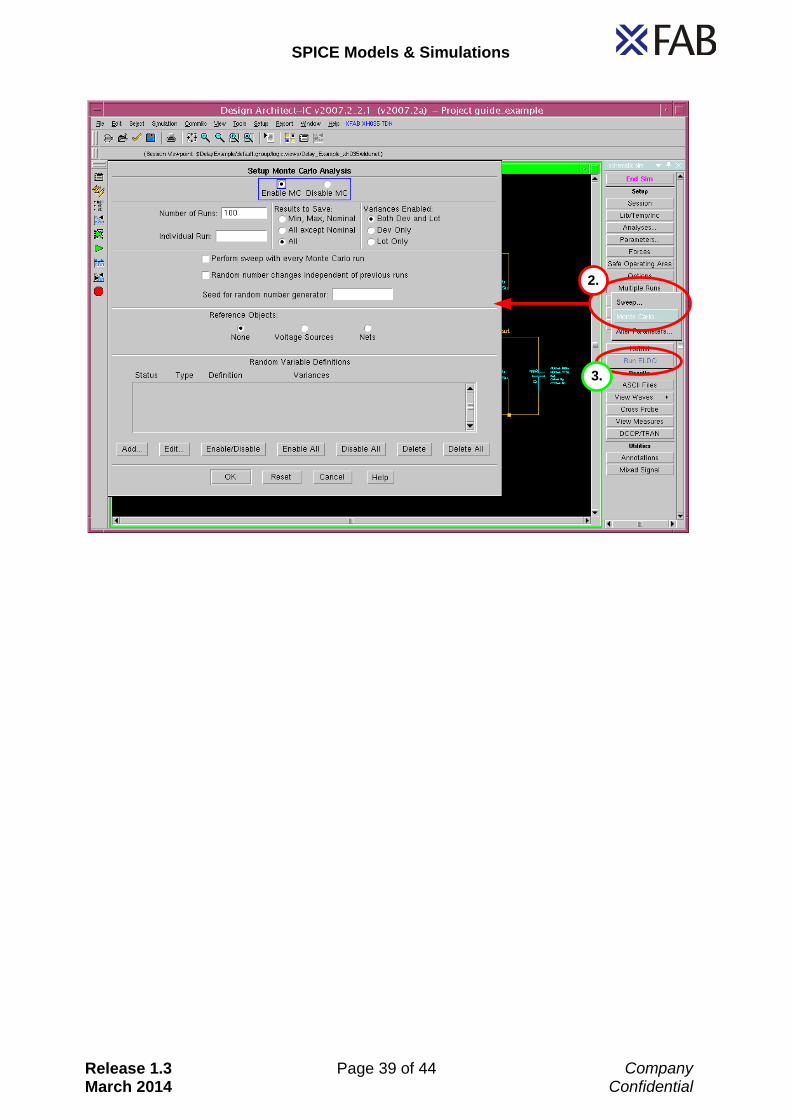
2. open ‘Setup Monte Carlo Analysis’ dialogue from the ‘schematic sim’ menu
Multiple Runs → Monte Carlo …
Enable MC
set ‘Number of Runs’
choose type of parameter variation: ‘Both Dev and Lot’ → Mismatch & Process ‘Dev Only’ → Mismatch Only ‘Lot Only’ → Process Only
more options to control the simulation specifically
3. after setting up the usual stuff like ‘Analyses…’, ‘Measurements’ etc., start the
simulation from ‘schematic sim’ menu → Run ELDO
SPICE Models & Simulations
Release 1.3 March 2014
Page 39 of 44 Company Confidential
2.
3.
SPICE Models & Simulations
Release 1.3 March 2014
Page 40 of 44 Company Confidential
2.4.3 Operating Condition Check (OCC)
I. open ‘Set Library Paths’ dialogue as shown in paragraph 2.4.1 II. change model paths to occ models and add two more files:
1) tstep_occ.lib → define time step of checking interval in the ‘Section’ area
2) technology.occ (e.g. xh035.occ) → library with the VerilogA modules (Leave ‘Section’ blank!)
The structure of the library-directories, where to find the occ models and the additional files depends on the used technology: ≥0.6µm: …/technologyocc/module/bsim3v3.scs
… …/technologyocc/module/technology.occ …/technologyocc/module/tstep_occ.lib
≤0.35µm: …/technology/occ/module/bsim3v3.scs
… …/technology/occ/module/technology.occ
…/technology/occ/module/tstep_occ.lib
III. setup transient simulation and start it from ‘schematic sim’ menu → Run ELDO

SPICE Models & Simulations
Release 1.3 March 2014
Page 41 of 44 Company Confidential
2.4.4 Lot Specific Models (LSM)
I. open ‘Set Library Paths’ dialogue as shown in paragraph 2.4.1 II. include the following two files:
1) eldo_params.lib → which you already installed (see section 0)
2) technology.lib (e.g. xh035.lib) → choose the Library Variant lsm
III. setup transient simulation and start it from ‘schematic sim’ menu → Run ELDO
2.4.5 Pre-Layout Models With Parasistic Diodes/Capacitors (PLPar)
I. open ‘Set Library Paths’ dialogue as shown in paragraph 2.4.1 II. include the following two files:
1) param.lib specify the sigma (Lib Variant: 2s,3s,4s,5s,6s) → only for technologies ≤0.35µm
2) technology.lib or bsim3v3.lib, etc. from the specific directory:
…/technology/[simulator]/module/parasitics/technology.lib
→ choose the Library Variant (tm,wp,ws,wo,wz)
III. In some parasitic models, a global substrate node is used in addition to the device
nodes. → global node name: “psub“
This global substrate node must be connected to the device substrate node. IV. → Run ELDO

SPICE Models & Simulations
Release 1.3 March 2014
Page 42 of 44 Company Confidential
2.5 PSpice
If the model library is installed to the root directory of the hard drive I:\ no additional preparation is required. Otherwise all the paths to the files (technology_corner.lib and param_#s.lib), have to be adjusted to the actual installation path.
2.5.1 Corner Simulation
PSpice Corner Models are available for technologies ≥0.35µm. For Details see Table 1-1. In PSpice the corner names differ from the standard defined in paragraph 0:
standard PSpice tm tt0 wp ff4 ws ss1 wo fs3 wz sf2
Prepare your netlist *.cir: I. Choose a corner by including the specific library file .lib path_to\pspice\technology\module\technology_corner.lib
II. include param_#s.lib and replace # by number of sigma: # → 2,3,4,5,6 → only for technologies =0.35µm .lib path_to\pspice\technology\module\param_#.lib
Example: To simulate the corner ws (in PSpice: ss1) of the technology xh035 with module mos add the following statements to your netlist: .lib I:\pspice\xh035\mos\xh035_ss1.lib .lib I:\pspice\xh035\mos\param_6s.lib
→ only necessary in 0.35µ-technologies

SPICE Models & Simulations
Release 1.3 March 2014
Page 43 of 44 Company Confidential
2.5.2 Pre-Layout Models With Parasistic Diodes/Capacitors (PLPar)
I. Choose a corner by including the specific library file .lib path_to\pspice\technology\module\parasitics\technology_corner.lib
II. include param_#s.lib and replace # by number of sigma: # → 2,3,4,5,6 → only for technologies =0.35µm .lib path_to\pspice\technology\module\param_#.lib
III. In some parasitic models, a global substrate node is used in addition to the device
nodes. → global node name: “$g_psub“
This global substrate node must be connected to the device substrate node. PSpice Corner Models are available for technologies ≥0.35µm. For Details see Table 1-1.
SPICE Models & Simulations
Release 1.3 March 2014
Page 44 of 44 Company Confidential
Appendix
A References [1] Cadence
Virtuoso Analog Design Environment XL User Guide [2] Mentor Graphics
Eldo User’s Manual [3] Synopsys
HSPICE User Guide: Simulation and Analysis [4] Cadence (2007)
PSpice A/D Reference Guide (Product Version 16) [5] M. J. M. Pelgrom (1989)
“Matching Properties of MOS Transistors” IEEE Journal of Solid-State Circuits, Vol. 24, No. 5, 1433-1439
[6] GSA – Global Semiconductor Alliance (2005)
“Checklist Taxonomy & Definitions” www.gsaglobal.org
[7] Hoang Pham (2006) Handbook Engineering Statistics (1. edition) Springer
The information furnished herein by X-FAB Semiconductor Foundries is substantially correct and accurate. However, X-FAB shall not be liable to licensee or any third party for any damages, including but not limited to personal injury, property damage, loss of profits, loss of use, interruption of business or indirect, special, incidental or consequential damages, of any kind, in connection with or arising out of the furnishing, performance or use of the technical data. No obligation or liability to licensee or any third party shall arise or flow out of X-FAB´ rendering technical or other services. The X-FAB Semiconductor Foundries makes no warranty, express, statutory, implied, or by description regarding the information set forth herein or regarding the freedom of the described devices from patent infringement. X-FAB reserves the right to change specifications and prices at any time and without notice. Therefore, prior to designing this product into a system, it is necessary to check with X-FAB for current information. The products listed herein are intended for use in normal commercial applications. Applications requiring extended temperature range, unusual environmental requirements, or high reliability applications, such as military, medical life-support or life-sustaining equipment are specifically not recommended without additional processing by X-FAB for each application.


![PHASE-LOCKED LOOP SIMULATIONS USING T-SPICE Contents · Phase Lock Loop Simulations [1] PHASE-LOCKED LOOP SIMULATIONS USING T-SPICE Contents: • A Brief Introduction to T-Spice •](https://img.pdfslide.us/doc/110x75/5adfd3d67f8b9a1c248c7fb4/phase-locked-loop-simulations-using-t-spice-lock-loop-simulations-1-phase-locked.jpg)