APPENDIX I

Fundamentals of Stoichiometry of Complex Reaction Systems

Bioprocessing includes a large variety of metabolic reactions even on the macroscopic level (cf. Fig. 2.16) and at the same time is carried out in different modes of reactor operations. Therefore, complex reaction systems must be treated stoichiometrically, which means that not only complex reactions themselves must be considered but also complex reactor operations.

1.1 Stoichiometry of Complex Reactions

The stoichiometric equation in the case of complex reactions can be written in the form

while for a simple reaction the following form is valid:

where i = number of reactions (1 :::;; i :::;; M) j = number of components (1 :::;; j :::;; N)

Aj = components of reaction mixture v = stoichiometric coefficients

(U)

(1.2)

The differential change of the number of moles n of component Aj due to the reaction i is defined as

(1.3)

where ei is the extent of reaction, defined as the change of number of moles divided by the stoichiometric coefficient [mole].

In complex reactions, the singular reaction steps are interconnected, that is, singular components participate in different reactions, with the conse­quence that a part of the reactions is stoichiometrically dependent. Only the independent reactions can be determined from the change in the number of moles. The solution to the problem of stoichiometric dependence can be found

1.1 Stoichiometry of Complex Reactions 407

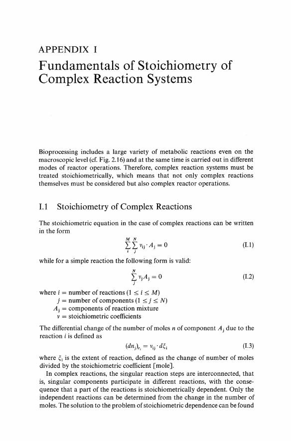
with the aid ofthe "matrix of the stoichiometrical coefficients" of the following structure

~ Components 1 ~ j ~ N

~ VI

VI (1.4)

where the row index is the number of reactions i and the column index is the number of components j. Each row of the stoichiometric coefficient matrix expresses the stoichiometry of a reaction in terms of the number of moles of each compound converted per unit reaction rate.

The number of stoichiometrically independent reactions is given by the rank of the matrix R p, which can be determined with e.g. the aid of the Gaussian method of elimination. As a result, the stoichiometrical coefficients of Rv linearly independent equations for the reaction system are necessary and sufficient for, for example, calculation of the conversion of the key variables and therefore also for all other components. Thus

(1.5)

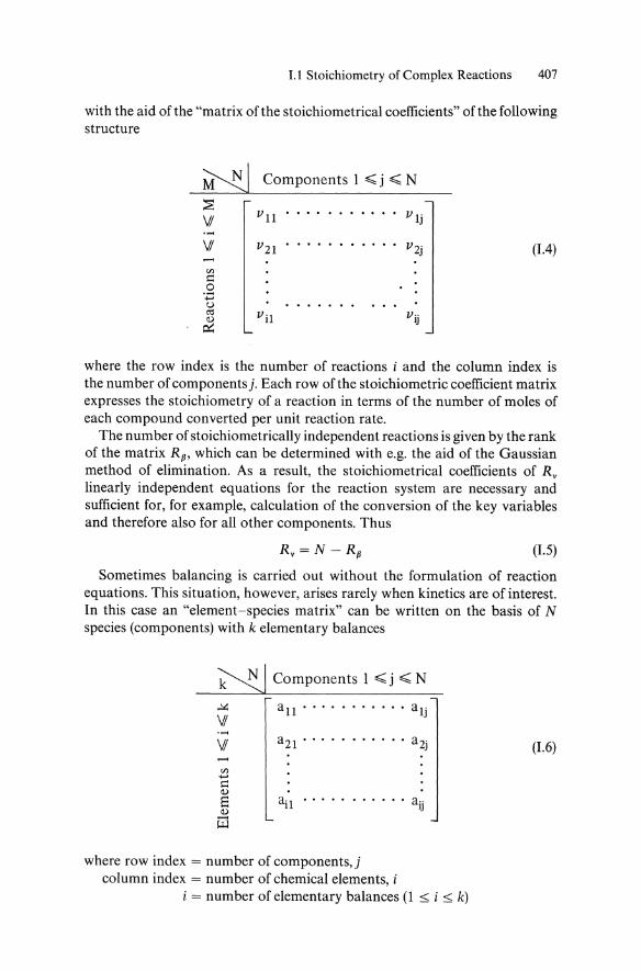
Sometimes balancing is carried out without the formulation of reaction equations. This situation, however, arises rarely when kinetics are of interest. In this case an "element -species matrix" can be written on the basis of N species (components) with k elementary balances

k'S1 Components I ~ j ~ N

..::.: all .... · ...... VI

VI a21 ... · .... ,. ..

en ....... ::: Cl)

E ~l ...... · ......

Cl)

G:l

where row index = number of components, j column index = number of chemical elements, i

alj

a2j

aij

i = number of elementary balances (1 ::;; i ::;; k)

(1.6)

408 I. Fundamentals of Stoichiometry of Complex Reaction Systems

aij = number of atoms of atomic species i present in molecule of componentj «resp. aj' bj , cj ' dj , etc.)

The number of key variables R is determined again with the aid of the rank of this matrix R. Thus (Schubert and Hofmann, 1975)

R = N - Rp (1.7)

Normally Rp = k in the case of N species and k elements. Hence, only (N - k) net conversion rates can be chosen independently.

From this reasoning it becomes clear that the number of independent kinetic equations to be postulated cannot be chosen at will-it is completely specified by the number of elementary balances k and the number of components N in the system (Roels, 1980). Which key variable or which kinetic equation is to be chosen strongly depends on the application one has in mind.

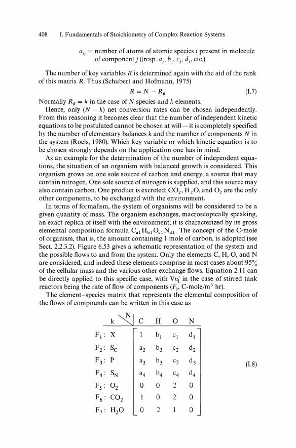
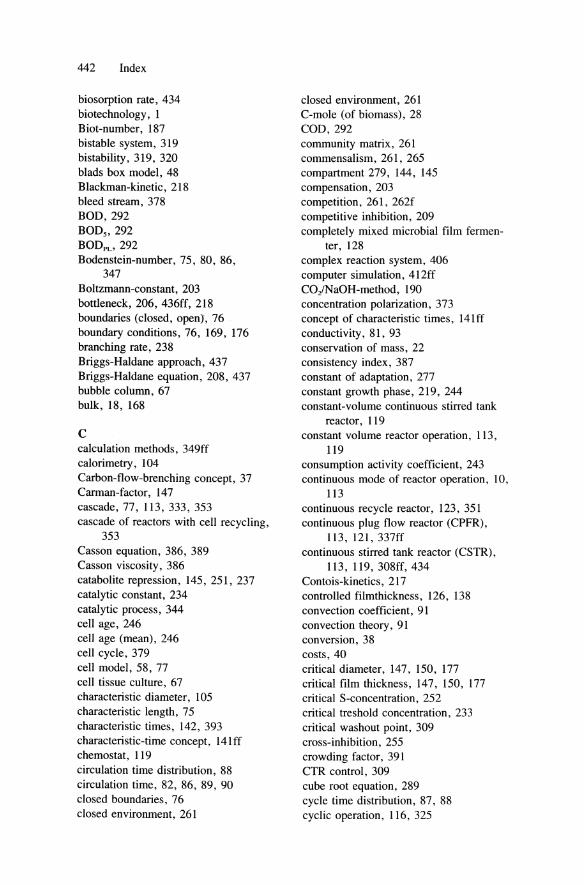
As an example for the determination of the number of independent equa­tions, the situation of an organism with balanced growth is considered. This organism grows on one sole source of carbon and energy, a source that may contain nitrogen. One sole source of nitrogen is supplied, and this source may also contain carbon. One product is excreted; CO2 , H 2 0, and O2 are the only other components, to be exchanged with the environment.

In terms of formalism, the system of organisms will be considered to be a given quantity of mass. The organism exchanges, macroscopically speaking, an exact replica of itself with the environment; it is characterized by its gross elemental composition formula Cal Hbl 0Cl Ndl . The concept of the C-mole of organism, that is, the amount containing 1 mole of carbon, is adopted (see Sect. 2.2.3.2). Figure 6.53 gives a schematic representation of the system and the possible flows to and from the system. Only the elements C, H, 0, and N are considered, and indeed these elements comprise in most cases about 95% of the cellular mass and the various other exchange flows. Equation 2.11 can be directly applied to this specific case, with Vn; in the case of stirred tank reactors being the rate of flow of components (Fj' C-mole/m3 hr).

The element-species matrix that represents the elemental composition of the flows of compounds can be written in this case as

k~1 C H ° N

F I : X bi ci d l

F 2 : Sc a2 b2 c2 d2

F3 : P a3 b3 c3 d3 (1.8) F 4 : SN a4 b4 c4 d4

F5: °2 0 0 2 0

F6: CO2 0 2 0

F7: H2O 0 2 0

1.2 Example for Determination of Number of Linearly Independent Equations 409

In the present case there are seven flows, and Equ. 2.11 specifies four equations between the flows represented in the matrix of Equ. 1.8. Hence, only three flows are independent variables (cf. Sect. 1.2). Which kind offlows to be chosen for measurement depends on the possibilities for experimental determination. The knowledge, for example, of the respiratory quotient and the ratio of oxygen consumption to substrate consumption allows direct estimation of the biomass production rate and the product formation rate. This conclusion from the application of balancing is of the greatest importance in situations where process variables, for example, X, are very difficult to measure, which is the case in penicillin fermentation (Mou and Cooney, 1983).

1.2 Example for Determination of Number of Linearly Independent Equations ("Key Reactions")

Reaction scheme

Reaction steps

VA 'CA + VBl'CB ~ VCl 'Cc

VCl 'Cc~ VA 'CA + VBl 'CB

VC2 • Cc + VB2 • CB ~ Vo' Co

Vo • CD ~ VC2 • Cc + VB2 • CB

(1.9a)

(1.9b)

(1.9c)

(I.9d)

(1.ge)

(1.9f)

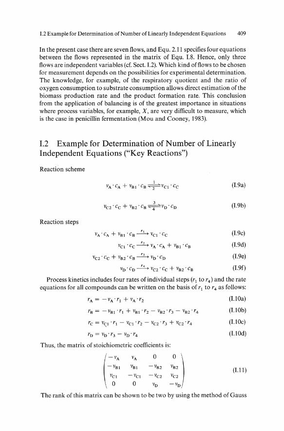
Process kinetics includes four rates of individual steps (r 1 to r 4) and the rate equations for all compounds can be written on the basis ofrl to r4 as follows:

rC = V<;:l • r l - VCl • r2 - VC2 ' r3 + VC2' r4

ro = vO'r3 - vO'r4

Thus, the matrix of stoichiometric coefficients is:

o

(1.1Oa)

(1.10b)

(1.10c)

(1.10d)

(1.11)

The rank of this matrix can be shown to be two by using the method of Gauss

410 I. Fundamentals of Stoichiometry of Complex Reaction Systems

elimination or by finding the order ofthe determinant, which is not zero. Thus, for example, the second column is identical with the first when multiplied by -1; the same with the fourth and the third columns. The remaining matrix is then

(~ o 0) -Va2 0 -VC2 0

VD 0

(1.12)

With Rp = 2, the number of key reaction or key variables is two, and these can be chosen arbitrarily (e.g., A and D). Thus the remaining dependent rates can be written on the base of rA and rD :

(1.13a)

(1.13b)

1.3 Stoichiometry of Complex Reactor Operation

The majority of stoichiometric considerations is restricted to closed reactor operations, where div (cjv) = 0, so that according to Equ. 2.3b

dc· _J = +v .. r dt - J

(1.14)

A simple case appears also with continuous stirred tanks.

13.1 SEMIDISCONTINUOUS REACTOR

For semidiscontinuous processing, often used in fermentations for the produc­tion of yeast biomass or secondary metabolites, the basic balance equation is to be modified. Balancing in this case has to distinguish between components that are already present in the reactor at the beginning (number of moles nj,o) and components that are fed later on to the reactor (flux of moles liY>- The stoichiometric balance in this case of semi discontinuous reactor operation is

where nj = number of moles of component j njO = temporal initial value of n nY = spatial initial value of n

(1.15)

This operation contains the time t as an independent process variable, in contrast to all batch reactor configurations.

1.3 Stoichiometry of Complex l{eactor Operation 411

1.3.2 NONSTATIONARY REACTOR OPERATION

Stoichiometry, for example, in the case of nonstationary modes of reactor operation, needs another fundamental equation. For the CSTR the balance of a component j is written as

dc· c· - cf! d~. d/ + Y = f vij de'

which gives after integration

cj = cY + (cj,o - cY)e-t/ f + I vij' ~*(t) i

where ~* is the modified extent of reaction.

(1.16)

(1.17)

Characteristically this equation contains again the time t as a process vari­able. This term with the time t disappears and can be neglected in the case of stationarity (if t » T) and when cj,o = cy, that is, in a batch reactor. Therefore the stoichiometric balance equation of a discontinuous system can be formally applied to a nonstationary continuous stirred tank. Similarly, the stoichiome­tric equations of heterogeneous reactor systems with interfacial mass transfer can be derived (Budde, Bulle, and Riickauf, 1981).

BIBLIOGRAPHY

Budde, K., Bulle, H., and Riickauf, H. (1981). Stochiometrie chemisch-technologischer Prozesse. Berlin: Akademie Verlag.

Mou, D.G., and Cooney, Ch.L. (1983). Biotechnol. Bioeng., 25, 225, and 257. Roels, J.A. (1980). Biotechnol. Bioeng., 22, 2457. Schubert, E., and Hofmann, H. (1975). Chem. lng. Techn.,47, 191.

APPENDIX II

Computer Simulations*

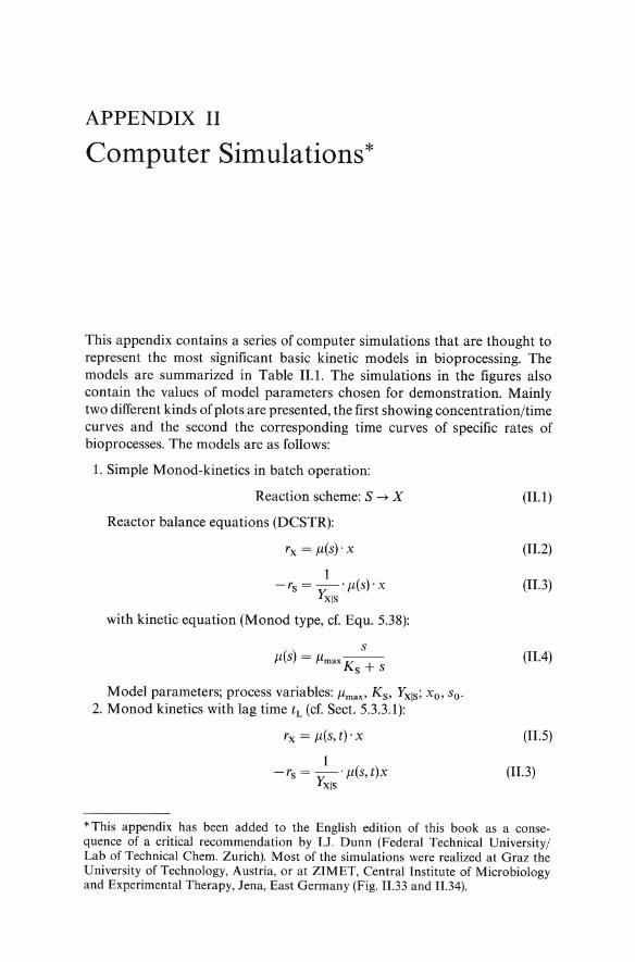
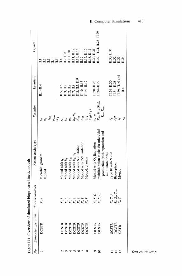
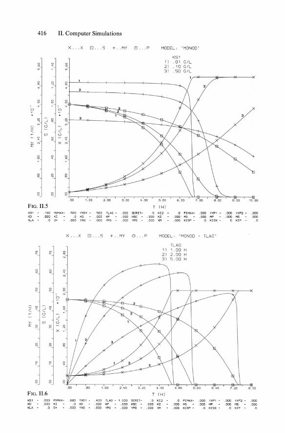
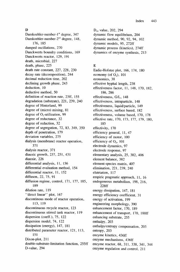
This appendix contains a series of computer simulations that are thought to represent the most significant basic kinetic models in bioprocessing. The models are summarized in Table 11.1. The simulations in the figures also contain the values of model parameters chosen for demonstration. Mainly two different kinds of plots are presented, the first showing concentration/time curves and the second the corresponding time curves of specific rates of bioprocesses. The models are as follows:

1. Simple Monod-kinetics in batch operation:

Reaction scheme: S ~ X

Reactor balance equations (DCSTR):

rx = fl(S)' x

1 - rs = -' fl(S) . x

YX!S

with kinetic equation (Monod type, cf. Equ. 5.38):

S

fl(S) = flmax Ks + S

Model parameters; process variables: flmaX' Ks, YX!S; Xo, So· 2. Monod kinetics with lag time tL (cf. Sect. 5.3.3.1):

rx = fl(S, t)· x

1 -rs = -' fl(S,t)X

YX!S

(II.1 )

(1I.2)

(11.3)

(11.4)

(11.5)

(11.3)

*This appendix has been added to the English edition of this book as a conse­quence of a critical recommendation by 1.1. Dunn (Federal Technical University/ Lab of Technical Chern. Zurich). Most of the simulations were realized at Graz the University of Technology, Austria, or at ZIMET, Central Institute of Microbiology and Experimental Therapy, lena, East Germany (Fig. II.33 and II.34).

TA

BL

E I

LL

Ove

rvie

w o

f sim

ulat

ed b

iopr

oces

s ki

neti

c m

odel

s.

No.

B

iore

acto

r op

erat

ion

Pro

cess

var

iabl

es

Kin

etic

mod

el t

ype

Var

iatio

n E

quat

ions

F

igur

es

DC

ST

R

X,S

M

icro

bial

gro

wth

: S

o IL

l-II

.4

II.!

M

onad

X

O

II.2

Y X

IS

11.3

/lm

ax

II.4

K

s II

.S

2 D

CS

TR

X

,S

Mon

ad w

ith

tL

tL

II.S

, 1I

.6

II.6

3

DC

ST

R

X,S

M

onad

with

kd

kd

II.3

, II

.7

II.7

, II

.8

4 D

CS

TR

X

,S

Mo

nad

wit

h m

s m

s II

.2, 1

I.8

1I.9

, IU

O

5 D

CS

TR

X

,S

Mon

ad w

ith k

d,

ms

k d,

ms

II.7

, II

.S

11.1

1, 1

1.12

6

DC

ST

R

X,S

M

on

ad w

ith S

inhi

biti

on

K,s

II

.2, 1

I.3,

H.9

II

'!3,

II.

!4

7 D

CS

TR

X

,S

Mon

od w

ith

2-S

lim

itat

ion

KI2

II

.10-

II.1

3 11

.15

8 D

CS

TR

X

,S

Mon

ad:

diau

xie

Scr

it

11.1

4-II

.19

ILl6

, IL

l 7

KI2

(KR

) II

.1S,

II.

! 9

,....

kLia

H

.20

-II.

23

II.2

0, I

I.21

~

()

K,p

, K

,sp(

KR

),

II.2

4-I

1.29

II

.22-

II.2

4, n

.25

-II.

29

0

Kp,

K,s

x 3 '"d

9 D

CS

TR

X

,S,O

M

onad

wit

h O

2 li

mit

atio

n 10

D

CS

TR

X

,S,P

; m

ulti

inhi

biti

on m

odel

for

mic

robi

al

prod

ucti

on (

with

rep

ress

ion

and

I:: .....

mul

tiin

hibi

tion

s)

Fs

1I.2

4-11

.30

II.3

0, 1

1.31

<1

l ... 11

S

CS

TR

X

,S,P

T

ype

10 w

ith

S fe

ed

cJt

11.3

1-11

.38

II.3

2 t/

) a' S

o 11

.39,

11.

40 a

nd

11.3

3 I::

Xo

1I.4

II

.34

§: o·

12

DC

ST

R

Sc,

Sd'

Sad

s B

ioso

rpti

on

13

CS

TR

X

,S

Mon

od

::l

;;;l

en

~

-!:>-

,....

w

r-, <:> ~

S·

::: ~ '" ::=

414 II. Computer Simulations

x ... X (C) •• • S + . . MY C) . . . p MODEL : '1'10 00 '

SO 0 0 0

1 1 . S GI L ~ a: . 2 ) 1 . 0 GIL "' 3) 2.0 GIL

0 0 0 a: 0 ...

0 0 0 3 0 0 0

~ 3 0

0 0 0 ... :::: "' :::: ., M

Cl Cl I ....

Ul X " lil ill d

>- N L

2

ill " 0

'" .

'" 0' . ~

:5 ~ 0

"! . 00 1.00 q . DO 5.00 8.00 , .00 9.00 9 . 00 10 DO

FIG. 11.1 T (H)

K51 .100 I1YHAX~ .500 'I'XSl .SOO TLAG - . 000 SCRIT - .0 KI2 .0 PIMAX - .000 YXP1 - .000 YXP2 - .000 KO .000 KI .0 KO .000 KP .000 K5C - .000 KZ .000 HO .000 He .000 HS .000 KLA .0 O· .000 YXO .000 YPO .000 YPS - .000 XH .000 KISP - . 0 KISX - .0 KIP - . 0

X . .. x (C) ••• S + . . MY 0 ... p MODEL: 'MONaD'

xo 0' "

, 1) .01 GIL '" . a: 2) .os GIL OJ> 3) .10 GIL

" i'l ... a: . " n 0

" " '" ~

!;: ~ " ~ W a:

'"' Cl <.:> r

Ul x 0 ill ill .

>- N L

:il 0 ;;. . " ~ a:

0 0 0 0 0 0

. 00 1.00 2 . 00 3 . 00 4 . 00 5 .00 6.00 , .00 9.00 9 . 00 1Q , OC

FIG. 11.2 T (H)

<51 '00 MYMAX- .soo YXSl 500 TLAG - .000 SCRIT - .0 KI2 . 0 PIMAX - . .000 YXP1 - .000 YXP2 - .000 <D . 000 KI . 0 KO 000 KP . 000 K5C .000 KZ . 000 HO .000 He .000 H5 .000 <LA . 0 O· .000 YXO .000 YPO .000 YPS . 000 XH .000 KISP - .0 KISX - .0 KIP - .0

II. Computer Simulations 415

x ... X eJ . .. 5 + . . MY (') • .. 1" MODEL: '''10 00'

YXS'

Ii! <> 11 .20 . ~ 2 ) . 50

iii 3) . 70

fi! ~ '" ~

c <> ~ c <>

0

~ ::: <> ::: m

'" . '"' <.:l <.:l

I .... Ul X

<> <> II! . .. >- ..; I:

<> :i' '" "'

~ j;: ("!

<> <> <> <> <> c

. 00 1.00 2 . 00 3 . 00 4 . 00 5 . 00 6 .00 7 00 B 00 9 . 00 10 , 00

F IG. 11.3 T CH)

KS1 100 MYMAX- .500 YXS1 .500 TLAG - . 000 SCRIT - .0 KI2 . 0 PIHAX - . 000 YXP1 - .000 YXP2 - .000

KO .000 KI . 0 KO . 000 KP .000 Kse .000 KZ .000 HO . 000 "" .000 MS .000

KLA .0 O· .ODO YXO . 000 YPO .OOD YPS - .000 XM . 000 KISP - 0 KISX - . 0 KIP - . 0

x .. X eJ . .. 5 t- .. MY Cl .. . 1" MOOE"L : '''10''100'

& ~ "1YMAX

0-Il .20 I / H

~ '" 2) .50 I / H 31 .80 l/H

3 2

" <> 0- 3 , ... ..

'" <> <>

'" '" " 0

I !l' -: 0- !<: .. .... '"' 2 <.:l

:::. >- til <.:l L ill 0- :i' '" ><

~ c :i! . ("! ~ " "!

g c g c ., . 00 1 , 00 2 . 00 3 , 00 4 .00 5.ao 6 . 00 7 . 00 a 00 9 . 00 11) .00

FIG. 11.4 T CHl

<S1 ' 00 MYMAX - 500 YXS, 500 TLAG - . 000 SCRIT- .0 KI2 . 0 PIMAX- 000 YXPt .000 YXP2 - . 000 <D .000 KI .0 KD . 000 KP . 000 Kse .000 KZ .000 HO . 000 MP . 000 MS .000 KLA 0 O · 000 YXO . 000 YPO . 000 YPS .000 XM 000 KISP - . 0 KISX - .0 KIP . 0

416 II. Computer Simulations

x . .. X ~. .. 5 + .. MY (') . . . p MODEL : . MONDO '

KS1

" " " 1) .01 GIL

'" .. oD 2) .10 GIL '" 3) .50 GIL

0 " 0 a: ... a: . " " 0 0 0 0

~ 0

!l il !l 3 ...J

..; ..... '" " I -' ..... .....

(J) " 0 " 0' .. .. .. >- N x N I:

~ " " .. '"

~ f': " a:

" " " ~- " " . 00 1.00 2 . 00 3 . 00 4 . 00 S . OO 6.00 7 . 00 8 . 00 9 . 00 10 . 00

FIG. II.S T (H)

1(51 '00 MYMAX - .500 YXSl .500 TLAG - .000 SCRIT - . 0 KI2 . 0 PIMAX- .000 YXPl . 000 YXP2 - . 000 KD .000 KI .0 KO . 000 KP . 000 Kse .000 KZ .000 HO .000 MP . 000 MS . 000 KLA . 0 O· .000 YXO .000 YPO - .000 YPS .000 XM .000 KISP - . 0 KISX - . 0 KIP .0

X ... X ~ . .. 5 + .. MY (') . .. p MODEL: . MONDO . fLAG '

flAG

" " " 1) 1.00 H

~ ~ '" 2) 200 H N 3) S.OO H

" fjl " "! .. '"

~ " " ~ " 0

I " -' " :i: .. .. ..... ..... (?

-' ..... >- Ul <.::> E co " " n ... N

X -f': " " N a:

~ ~ " ..

" " " " ~ . 00 . 80 1.60 '2.40 3 . 20 4 . 00 4,ao 5 .60 6 . 40 7 . • 0 8 . 00

FIG. 11.6 f ( Hl

KS' .003 MYMAX- .680 YXSl , Il03 TLAG - 1.000 SCRIT- .0 KI2 .0 PIMAX - . 000 YXPl - .000 YXP2 - 000 KD .000 KI .0 KO .000 KP .000 Kse . 000 KZ 000 MO .000 Me . 000 MS . 000 KLA .0 O· .000 YXO .000 YPO . 000 YPS .000 XM . 000 KISP - .0 KI SX - . 0 KIP - .0

II. Computer Simulations 417

x . .. X C!l •• S .,. .. '1'1' O. '" ..,OOt'L · ''''0'100 1(0 '

1(0 1 1 .00 1 l>-l

a 5; ... 21 .02 1 '>-l

11 .10 1 l>-l

~ ~ .0 0:

'"

~ <> ~

.J " " . -:: ~

..... (,) (,)

(Jl X 0 a '" .

N

a " "' oD

a a 3

"' '"

" a " .00 2 . 00 ~ , I'}D 6.00 a . ~o 10 .00 121)0 1A . 1)0 1S.t}Q 19 ':)0 20 ~o

FIG. II.7 T (Hl

K51 .100 MYMAX - 350 YXSl . aDo TLAG - .001) SCRIT - .0 K12 .0 PJMAX - .000 YXPl - . 000 YXP2 - 000 KD . 100 Kl .0 KO .000 KP .000 K5C .000 KZ .000 HO 000 MP .000 H5 000 KLA . 0 O· 000 YXO . 000 YPO .000 YPS 000 XM . 000 KISP - 0 KISX - . 0 KIP

X ... X rI . .. S + . . MY C!l .. P MODEL, 'MONOD • KD '

KD 1) .00 l/H

:;: 2) . 02 l/H . 3) . 10 l/H

:il M

" " M 0

" . " ~ a .,

>- -L:

" ...

1 2 3

" " .00 '2 .00 4 00 6 . 00 B . OC! 10 . 00 12 . 00 14 . 00 16 00 18 . 00 20 , 00

FIG. II.8 T [Hl

KG1 100 MYMAX- 350 YXS1 .aoo TLAG - 000 SCRJT- .0 K12 0 PIMAX- .000 YXP l . 000 YXP2 - .000 KO .100 Kl 0 KO .000 KP 000 K5C .000 KZ .000 MO 000 MP .000 HS .000 KLA 0 O· .000 YXO .000 YPO .000 YPS .000 XM . 000 KISP - 0 KISX - .0 KIP 0

418 II. Computer Simulations

x ... X I!J . . .S . MY C) .. • p MODEL: . MONaD . MS '

MS

!:: li: 1) .00 l/H 2) .03 l/H .,; 3) . 10 l/H

li: ~ cO .

-X I X 2

~ <> X 3 <> .,

.J Q

.J <> . N .... ..; .... M

<::> <::>

(f) :J x <> . "

<> <> ~ N "' M

Q

"' 3 ~1

<> ~" '" 51 51 51 EJ , :1)0 2.00 3:00 A. OO 5.00 g , I)O 7 00 R OO 9 ,00 10 em

FIG. 11.9 (H l

K51 '00 MYMAX - 350 YXS1 dOD TLAG - 000 SCRIT - 0 KI2 0 PIMAX - 000 YXP1 000 YXP2 - . 000 KD .000 KI . a KO . 000 KP 000 KSC ODD KZ 000 MO 000 MP 000 M5 '00 <LA . 0 o· .000 YXO 000 yPO 000 yPS 000 XM 000 KISP - 0 KISX - 0 KIP a

X .. . X I!J . .. S + . . MY c.J . .. P MODEL: ' MONOD . MS '

MS 1) .00 l/H

!:: 2) .03 l/H 3) .10 l/H

li: M

Q Q

0 M

<> . ~

'!: <> m

>- -I:

:;,:

<> ~

3 2 1 <> <>

. 00 " DO 2 . 00 3 . 00 4 . QO 5 . 00 6 00 7 00 e ' 0 9 . 00 10 00

FIG. II.10 T (H)

<51 '00 MYMAX - 350 YXS1 ADO TLAG - 000 SeRIT - 0 <12 .0 PIMAX - 000 iXP1 . 000 l'XP2 - . 000 <0 .000 KI 0 KO ODD KP 000 K5e DOD KZ 000 MO DOD MP .000 MS '00 <LA 0 O' 000 YXO ODD YPO 000 YP5 000 XH ODD KISP - .0 KISX - 0 KIP .0

x . . X C!J. . S + .MY (') . . P

" " ... '" ; II)

" " "! ~

'" ~

" " " "

~ ~ .J " '" .; .... ..; <.) <.)

Ul x lil " .

N

~ " .. ..;

" " "! a;

g " '" 3 . 00 ILtlO

FIG. 11.11 T

KS' '00 MYI1A:( - . '350 YXS 1 ,a.oo TLAG - .000 SCRIT- .0

KO . 050 <I .0 KO .000 KP .000 KSC . 000

<LA . 0 0 ' .000 YXO .000 YPO - . 000 YPS . 000

X ... X C'J •. . S + .. MY (') .. . p

" '" ..;

" " M a

" . " ~

" ~ )-

:E

~

~

" " .00 1.00 2 . 00 3 . 00 · . 00

FIG. 11.12 T

K51 . 100 MYHAX- .350 YXS1 .400 TLAG - .000 5CRIT - .0

KD .050 KI .0 KO . 000 KP .000 KSC .000

KLA . 0 0 ' .000 YXO .000 YPO - .000 YPS - .000

II. Computer Simulations 419

MODEL, 'MONDO • KO • MS ' KO MS

1) .02 .03 l/H 2) . 02 .10 l/H 3) .10 .03 l/H 4) .10 .10 l/H

r-------___ -==2

S.on 6 . 00 1 00 8 . 00 9 . 00

(H)

KI2 . 0 PIHAX - .000 YXP1 .000 YXP2 -

KZ .000 MO .000 MP . 000 MS

XM .000 KISP - .0 KISX - .0 KIP -

MODEL, 'MONDO . KD . MS ' KD MS

1) .02 .03 l/H 2) .02 .10 l/H 3 ) .10 .03 l/H 4) .10 .10 l/H

2 • 3

5 .00 6 . 00 7 . 00 8 , 00 g.oo

(Hl

3

•

10 . 00

.000

.050 . 0

10 00

KI2 .0 PIMAX - .000 YXP 1 - .000 YXP2 - .000 KZ .000 MO .000 "" .000 MS .050 XM .000 KI SP - .0 KI SX - .0 KIP - .0

420

...J

~

'"

~

-~ cO

<> <> <Ii

<> . ui

" '"

" N

M

" '"

" "

FIG. n .13 1(: 1 'O{'"l <0 otJ'J KL 4 0

FIG. 11.14 10'9' '00 KD 000 ~LA 0

II. Computer Simulations

x . .. X ~ .. . -' + .. M."

" ~ "-

<> <> <0

<> <> on

:2 " '" l' x

g

" " - "--.--, ... 2 10 . ~, 6 ~~

M"'1A!(- 3S0 f"<-" soc TLI\" 000

" 2.0 1<0 1)1"10 "P 000 o· t;1)t) " >:0 01)0:' (DO 000

x . . . x ~ . . . : +

" N

<>

"'

<> <>

'" 0

<> . '"' ~

~ >- -:>::

~

" '"

" <> ." .00 ~ . ".I"; 4 .00 G 00

M:'MA::Z- 350 '(7..;3+ - ,SOD ruv:; 000 KI 2 .0 KO 000 KP ODD o· ODD YXO - ODD YPO 000

C!l ••• r>

" 00

SCRI f- a KSC 000 y p .; . 1)01)

(') .. P

3

~ ro

T ~~CRTT - 0 KSC oeD ypS oeo

MODEL: ' S-INHIRITION '

KIS 1) s.n GIL 2) 10.0 GIL 31 SO.O GIL

'0 "" 12 . QI) 14 . 00

(H)

Kf.-: . a PIMA>:: - .000 KI 001) MO 000 XM . 000 KlSP . 0

' 6 00

Y'':P1

MP K : ;3X

MODEL: ' S-INHI BI TION'

KI 1) S.O S/L 2) 10.0 S/L 3 1 50 . 0 r;/ L

2

' 0 . 1)1) ' 2 .~0

[H)

¥.I~ 0 PI/"IA)( -

"Z 000 MO XM OCr) KISP

,oa .!)/) 16 (II)

000 y'.;r> 1

000 MP 0 KISX

Hi 00 20 00

000 YXP:? 000 ,1)00 MS 000

0 KIP 0

19 QI) 20 QO

0(1[' YXP.~ rr;f)

000 MS 000 0 «:TP . 0

II. Computer Simulations 421

x ... X ~ .. .5 +. .MY (!) ... 52 MODEL, '2 -S-MONOO '

KI2

" " " 1) 1.0 GIL .. e- ll) ~ 2) 10.0 GIL

" ~ ~ " " . "' " " " " " " a: " on

" 0

..J " ~ 1& " ..J " "' ~ .... .... Q " -:! '" >- " x (Il Ii! I: W ~ " " (I] -

., ,-: c c . ~ '"

" !!' " ~ '" . " " " " " " " "

. 00 .80 1.60 2 . 40 4 .00 4.80 5 .60 8 .00

FIG. 11.15 T (H )

KS 1 .005 HYMAX- .670 YXS1 - ,480 TLAG - .000 SCRIT- .0 KI2 1.0 PIMI\X- .000 YXP1 - .000 VXP2 - .000 KO . 000 KI .0 KO .000 KP .000 Kse .000 KZ .000 Me .000 MP . 000 MS .000 KLA .0 O' .000 YXO . 000 YPO - .000 YPs - .000 XM .000 KISP - .0 KISX - .0 KIP .0

X .. .X O . .5 1- . . MY C) ... p MODEL, 'DIAUXTE '

SCRIT 1) .OS Gil :z 0> $ 2) S.OO Gil '"

" g . . . "

so: '" " '" ... .;

~ :! " :! ~ :! '" Q Q

., "

(l (J'1 '>< ;: '" ;:< '"

"'

!l' '" !l' '"

. " ~ '" '"

" " " " " " .00 .u. . C1C1 9 .00 12.00 16 . 00 20 , 00 24 , 00 <9 . 00 32. 00 36 . 00 11.0 . 00

FIG. 11.16 (H '

KS' 035 MYMAX- ,450 YXS1 '50 TLAG - 1.500 seRIT- a KI2 10.0 PIMAX - .225 YXP1 . 380 YXP2 - .590 KO .000 K! 8.0 KO 000 KP .050 Kse . 000 KZ .000 MO .000 MP .000 MS .000 KLA .0 O' .000 YXO 000 YPO .000 YPS .250 XM .000 KISP - .0 KISX - .0 KIP 8.0

422 II. Computer Simulations

X ... X 1!l ... S + .. MY (!) . . . P

Ii:

<> ~

0

~ M

I .... <> · ~ N

1:

<> 0

. 00 4 . 00 8 . 00 12 . 00 16 . 00

FIG. 11.17 KS' .035 MYMAX - , 450 YXS1 .150 TLAG - 1.1500 SCRIT -KD .000 KI 8.0 KO . 000 KP .050 Kse KLA .0 o· .000 YXO .000 YPO . 000 YPS -

X . . X I!l. .. S + . . MY (!) ... P

<> <> m <> ~ to :!.

<> <> · . <> · N ~

<> <> <> <> <> " to ~

-:! <>

.J <>

-:! ~ '" <> .... ai <:) l) l)

a. 1Il )(

:<: <> ~ <> .;

<> <> 'Ii ., <> .;

<> <> ~ . <>

"

0 0 <> 0 0 <>

. 00 11 . 00 8 00 1~ . OO 16 . 00

FIG. IU8 K5 1 . 035 MYMAX- . .:1.50 YXSl 'SO TLAG - 1.500 SCRIT -KO 000 KI 10.0 KO 000 KP 050 Kse KLA .0 0 ' .000 YXO 000 YPO 000 YPS

. 0 . 000 .250

MODEL, 'DIAUXIE'

SCRIT 1) . 05 GIL 2) 5.00 GIL

20 . 00 24 . 00 28 00

( HI

KI2 10 . 0 PIMAX- . 225 KZ .000 Me .000 XH .000 KISP - 0

MODEL, 'DIAUXIE' KI2

1) . 1 GIL 2) .5 GIL 3) 1.0 GIL 4 ) 2.0 GIL

20 . 00 24 . 00 28 00

T (HI , K12 2 . 0 PlMAX- 225

000 KZ 000 HO . 000 .250 XH 000 KISP - 0

321)1) 36.00 tl.0 . 00

iXP1 . 380 (XP2 - .1590 MP 000 "5 .000 K!SX - .0 KIP 8. 0

32 . 00 36 , 00 110 , 00

YXP1 - .380 VXP2 - 590 HP 000 HS 000 KISX - 0 KIP 20 . 0

II. Computer Simulations 423

x ... X [!) .. . S +. .MY C) ... I" MODEL. 'DIAUX1E' 1(12

11 .1 GIL 0

21 .5 GIL

'" 3) 1 .0 GIL ~ l 2.0 GIL

1£

0 0

#

0

:<: ..;

~ :;'

>- ..; :E

0 .. 0

"!

0

. 00 0. . 00 a 00 12.00 16 . 00 20 . QO 24 . 0{] 29 00 32 . 0D 36.QO 40 .00

F IG. 11.19 T (HI

KS ' .035 MYHAX- ,450 YXSl 'SO RAG - 1 sao SCRIT - , KI2 2.0 PIMAX - . 225 YXP, - .380 YXP2 - S90

KD . 000 KI 10.0 KO OOD KP .050 KSC .000 KZ .000 MO . 000 "" . 000 HS .000 KLA .0 O' . 000 YXO . 000 YPO - . 000 YPS . 250 XH . 000 KISP - . D KISX - .0 KIP 20 . 0

X ... X [!) .. .S + .. MY C) ... 1" MODEL. . OTR- LIMIT A TION'

, 0 0

'" " '"

... 0 0 , "

,

" il 0 0

" " S'

>'

!l' ::: 0 ::: 0

" "' () a: ()

,J , () CI' '" 111

<0 :<: 0

0 '"

:1. " 0 co ., "

C- o 0 co .

0 co 0

" co 0

.00 a.Clo '6 .00 24 . 00 32 . 00 40 ,00 48 , 00 58 . 00 64 .00 n .oo ao .oo

FIG. 11.20 T (HI

K5 1 000 MYMAX- .10tl. YXSl 200 TLAG - . 000 SCRIT - . D KI2 .D PlHAX- . 000 YXPl . 000 YXP2 - .000 KD 000 KI .0 KO .00 1 KP .000 KSC ' 00 KZ . 000 MO .000 MP .000 MS . 000 <LA 10.0 O' .008 YXO . 880 YPO .000 YPS .aoo XH . 000 KISP - .0 KISX - .0 KIP . 0

424 II. Computer Simulations

x . . .X ICI ... S + .. MY (') ... P MODE L, 'OTR-LIMITAT ION '

'<LA 0

11 10 1/H . 21 30 1/H 31 250 1/H

0

"

0 0

0

0

'" I ,

>-L

0 . 0

"

'" 0.

. 00 8 .00 16 IJO 24 00 32 . 1')0 40 ")0 .a8 . ")0 56 00 "" 00 7} ,10 91 'l'l

FIG. 11.21 rf-jl

KS' 000 I1),MAX - 'a" 1'X5 1 200 TLAC - 000 seQ! r- a <12 0 P I I1AX - 000 iXP1 000 n:P 2 - IJ~ Q

<a 000 <I . D <0 . 001 <P . ODa <so ' aD <l OOD " 0 ODD "" 000 M5 'J(; 'J

<LA 10 . 0 0 ' 008 YXO AAO YPO ODD 'P5 . 000 '" ODD '< ISP - 0 '( 15)( a <1 P a

X ... X ICI . . . S + .. MY (') ... P MODEL, ' MULTI-INHI BIT ION '

'<IP 0 0 '"

11 . 2 GIL '" 0 c 21 2 . 0 GIL

~ ;; 3 1 50.0 GI L

0 0 0 . '" '" '" ~ ~

'" 0

'" '" .... 1':

~ ~ ~ '" 0

el el e

a. (fl x ~ '" 0

~

" n

'" '" Q)

'" <-. '"

c " '" '" . 00 , 00 2 00 3 00 • 00 5 . 00 6 . 00 7 00 8 00 9 00 10 ,00

FIG. 11.22 T (f-jl " 0 ' KS ' - 2.000 '1'1'111\ >(- . 020 fXS' 7SD SCfED- 0 ~EED - 0000 VD 30 . 0 P!MAX - . 003 ,(XP l .000 YXP2 DDD <0 . 00 1 <I . 0 <0 , 000 <P 500 <50 . 000 KZ . 000 MD . 000 MP .000 M5 . 0 10 <LA - 500 . 0 o· 000 YXO . 250 ,"" - 0 . 250 iDS "D XM . 000 K!SP - 30,0 KISX - 80 . 0 KIP 20 . 0

x . .. X [!J ••. S + . . ""Y

" " .. .. ..; ..;

" " . . '" '"

" " " " '" N '" 0 0

" "!

::r ::r -... -...

l'l l'l qp - jJ - 3

" " P

<D II!

" ;: . " " " ~

. 00 1.00 2 . 00 3 . 00

FIG. II.23 K51 - 2.000 MYMAX~ .020 YXSl .750 SFEED - .0 KD .001 KI .0 KO .000 KP .500 KLA - 500.0 O' .006 1xa 1.250 YPO - 6.250

C). .. P

II. Computer Simulations 425

MODEL, . MUL Tr - INHIBIT ION '

I(IP 1) .2 GIL 2) 2.0 GIL 3) 500 GIL

4: . 00 $ . 00 6.00 7 .00 B. OO g . OO

T CHl _10 1

FEED - .0000 VO 30.0 PIHAX- .003 YXPl - .000 YXP2 -KSC .000 KZ .000 NO .000 ,., .000 MS YPS .710 XM . 000 KISP - 30.0 KISX - 80.0 KIP

l lC . OO

.000 010

20.0

X . . . X [:J ••. S + .. MY C) . .. P

!Ii " " .,

" " D· ... " ~ ; ~

!fI " " a " " " "' " ~ '" ~

N

~ " 0 " " " " " " <:> N ~ <:> " 0 " 0 '"

;: ..J " .,

" ..J " -... " "' . ..... " .. C) m <D C) ..q 2: ! -:!

(!)

qp : " jJ "' " X " D. " " cr; <>

"' ~ Ul

III " " :<l g " '" ..; iii

.., " ;- f.l " ., " " N

is " " g " " " ~ ,----,-----r .00 4 .00 8 . 00 12 . 00 16 . 00 2[1 DO 2rt . OO <9 .00 32 .00 36 . 00

F IG. 11.24 h -10' KS 1 2.000 MVMAX- .020 YXS1 , 75 0 TLAG - .000 SCRIT- .0 KI2 .00 PIMAX- .003 YXP1 - .000 YXF2 -KO .001 KI . 0 Ka .000 KP .500 KSC .000 KZ .000 MO .000 MP .000 MS KLA - 500 . 0 a· . a06 yxa 1.250 ypa 6.250 YPS - .7 10 XM .000 KISP - 30 . 0 KISX - BO.O KI P -

Llei . OO

. 000

.010 .S

426 II. Computer Simulations

g KP KI P KISP KISX

( I) 0.002 1.0 4 [I Il 0.020 1.0

iii ( III ) 0.002 10.0 [ IV ) 0 . 020 10 .0

~

'" "!

x <{

E N ~ a.. .... .....

a..

~

i<l

~

" " ,~~ :'0 , >0 . 30 . -0 ,so . &0 . 70 ,aD . '10 1.')0

FIG.II.25 '1Y/'1Y'1AX

xo 10.') SO - 100 .0 Y)(/S . £1.50 (P I S .gOO t1y!'1AX - .0920 PlMAX - . 0050 <5 . i SO 'is - . 1) 111') <0 - . !JOi O

. KP KIP KISP KI5X "

(I) 0 .50 200.0 1.0 1000 .0 200.0 10 . 0 4 1000.0

'" 0.50 20 1000.0 0 ,50 200.0 1000.0 1000.0

'" X ~,

is

x <{ :r: ~ ..... a.. .... ..... a..

!ZI

~

!" 2

" " , DO . '0 . 20 , 3D .40 . 50 .60 .70 .aD .90 1,00

FIG. 11.26 MYIMYMAX xo 10.0 50 - 100 . 0 YX/S - . 750 VP/5 - . 7 10 MYMAX - .0200 PIMAX - .0030 K5 - 2 . 000 MS - .0100 KD - . 00 10

II. Computer Simulations 427

. 0 KP KIP KISP KISX

( I ) 0.05 200.0 80.0 1000.0 (II) 0 .50 200.0 80.0 1000.0

( II II 5.00 200.0 80.0 1000.0 ( IV) 50.00 200 . 0 80.0 1000.0

x ~

is

x -0:

5 " "! a. ..... -a.

II!

III 4

!:>

0 0

. 00 . '0 .20 .30 .<0 . 50 .60 , 70 .ao .90 1.00

F IG. II .27 MY IMYMAX

xo 10.0 50 - 100 . 0 YX/S - . 750 yP/S .710 MYMAX - .0200 fllHAX - .0030 K5 - 2.000 HS - . 0100 KD - .0010

. 0 KP KIP KISP KISX

( I) 0.50 0.2 80.0 1000 . 0 ( II) 0.50 2.0 80.0 1000 . 0

~ (III ) 0.50 20.0 80.0 1000 . 0 ( IV) 0.50 200.0 80.0 1000.0

X ~

~

x -0:

5 ~ a. ..... -a.

~

III

!:>

0 0

. 00 , '0 . 20 .30 ,<0 .50 .60 .7 0 .ao . 90 1.00

F IG. n .28 MY/MYMAX

xo 10 . 0 SO - 100 . 0 YX/S .750 YP/S . 710 MYMAX - .0200 PIHAX - .0030 K5 - 2.000 M5 - . 0100 KD - . 0010

428 II. Computer Simulations

. " KP KIP KISP KISX

(I) 0.5 80.0 80.0 100.0 (II) 0.5 80.0 80.0 150.0

;; (III) 0.5 80.0 80 . 0 200.0 ( IV) 0 . 5 80.0 80.0 500.0

X ?!

3

ill

x « I: !;l -n. .... -n.

~

~

!:'

" " . 00 . '0 .20 . 30 . <0 .SO .60 . 70 .80 .90 1.00

FIG. 11.29 MY/MYMAX

XO 10 . 0 so - 100.0 YX/5 - .750 VP/5 - .710 MYMAX - .0200 PIMA)( - .0030 K5 - 2.000 MS - .0100 KD - .0010

x ... X [!J ... S + .. MY (!) .. .P

F/VO

" 1, .0005 l/H 3

" g " " 2.')« .001 l/H re ~ III 3 , . l/H

" " g " " . 3 Cl; ~ ~

" c c

" 0 " c

~ ;i g 2

.J " " :::! g

" " (-, :4 m " <.:> '" .J Z .... - U

" c " a. " c X " ~ '" ~ r.n

g " " " " .; :4

" " " " " " " .. 's......

" " " ............. EJ.... _---+J 3

" " "! ~~ . 00 4 00 B. OO 12 . 00 16 . 00 :10 00 :24 .00 28 00 32.0D 36 . 00 110 . 00

FIG.II.30 h· lO' K51 2 .000 MYMAX- .050 YX5 1 750 SFEED· 500 .0 FEE:'"D - .O O2C "0 35.0 PIMAX- .003 YXP1 - .000 YXP2 .000 KD OD1 KI .D KO .000 KP 500 KSC .000 KZ .000 MO .000 MP .000 MS .010 KLA 500 .0 D· . 006 YXO 1. '250 H'O - 6.:.!SO YPS .7 10 XM . 000 KISP - 30 . 0 KISX - 50 .0 KIP 20.0

il> ~.

~ ~

'" " ~ " 6 "' Cl <>

",'

~ " .. I ~ ....

lit " N

qp /J

~ ~ "

~ " d

" g "

. 00 4 . QO

FIG. II.3\ KSI . 2 . 000 MYMAX- .050 YXS1

KD .001 KI .D KO KLA - 500.0 O' . 006 YXO

S'

.:! u

(Jl

{ ~ sads

SAOS.MAX c> . <> '"

.00 '0

FIG. 1132 - 23 . 10 "I - 30 .00

e.e'J 12 , QO

.750 SFEED- SOO.O

. 000 KP SOD 1 . 250 1PO - 6 .250

20

II. Computer Simulations 429

FIVO

1 , .0005 1/H 2 , . 001 1/H 3 : . 002 1/H

; ! C ; IS .ao 24 . 00 28 . 00 32.00

h .10' FEFD - .0020 vo 35 .0 PIMAX- .003 YXP1 -KSC .000 I'.Z .000 HO .000 HP YPS .710 X" .000 KISF' - 30 . 0 KISX -

810 sopp r IO"I

. 50 .60 .70 . 90

T (H l

; ~.OD

.000 YXP2 -

.000 HS 50 . 0 KIP

. 90

01 - .5000 SRMAX - . 1730 - 1.210 K - 1 . 160

! ~ "0 ,00

000 . 010 20 . 0

1 ,00

430 II. Computer Simulations

----- - - --------------- -------- --~~;l 's So ' (g.' -')

------ -- ---- ---------- ----- -----r-------.8

------ ---- ------ --------- ------.~------.6

.5

_---;-.6 _____ ~ ., ~,

~1 o ~ -=-=-=-=-=-=--'::-=--="-::::~'""2_=:::_==:=-.::..:-::.;--=-~-~-..:.- .::..- .::..- -:::.:-:..:-:.:-..:.-l:::===::;j

o FIG. II.33

X

(go(')

.5

o

.5 D

UL ______________ ~ ________________ u

o 1- l00h

FIG. II.34

II. Computer Simulations 431

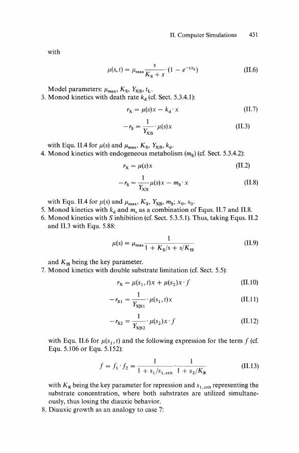
with

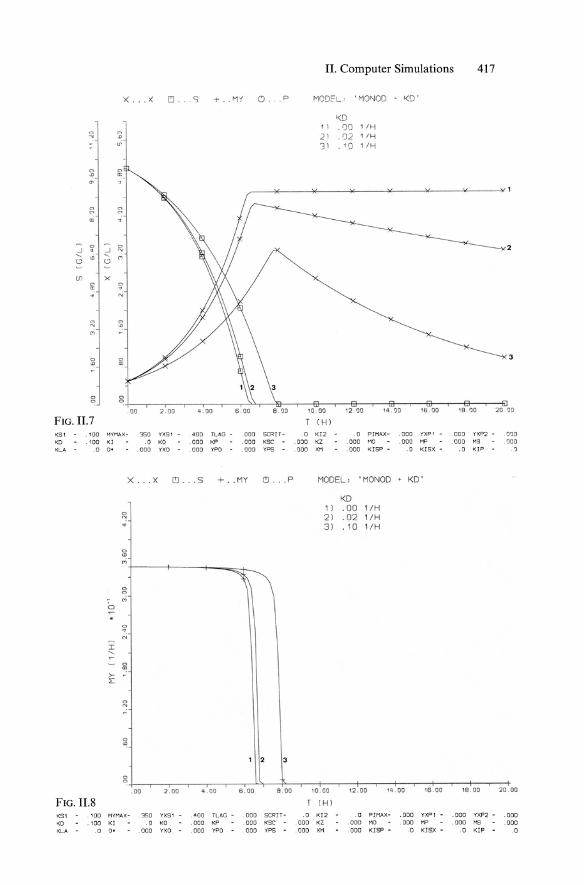
Model parameters: Jlmax, Ks, Yx1s, tL. 3. Monod kinetics with death rate kd (cf. Sect. 5.3.4.1):

rx = Jl(s)x - kd . x

1 -rs = -' Jl(s)x

Yxis

with Equ. 11.4 for Jl(s) and Jlmax, Ks, Yxls, kd •

(II.6)

(11.7)

(II.3)

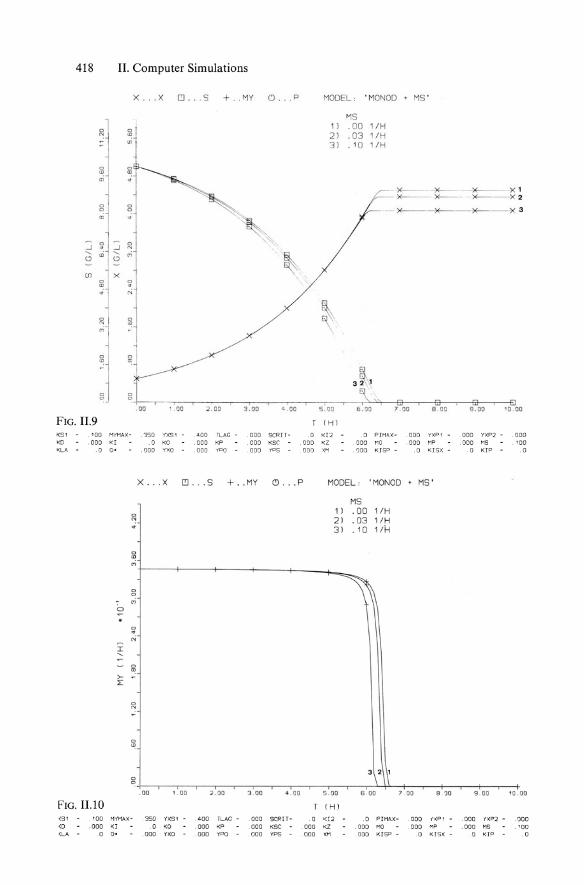
4. Monod kinetics with endogeneous metabolism (ms) (cf. Sect. 5.3.4.2):

rX = Jl(s)x

1 -rs = -Jl(s)x - ms' x

Yxis

with Equ. 11.4 for Jl(s) and Jlmax, Ks, Yxls, ms; xo, So·

(11.2)

(II.8)

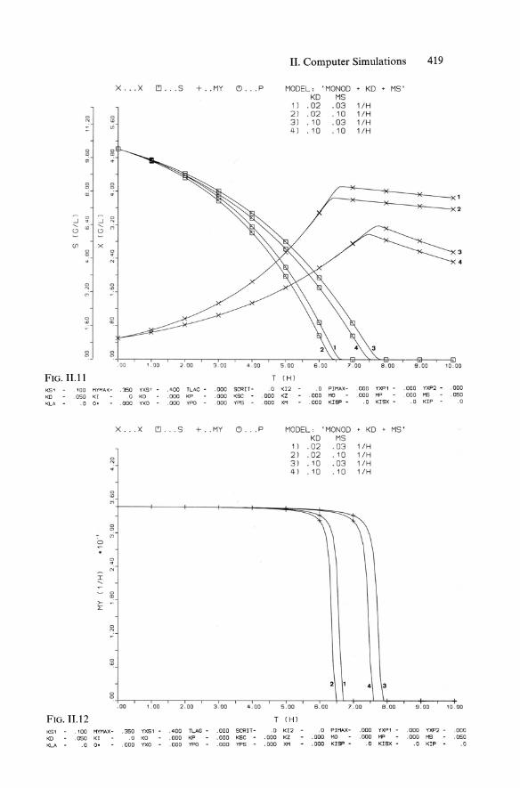
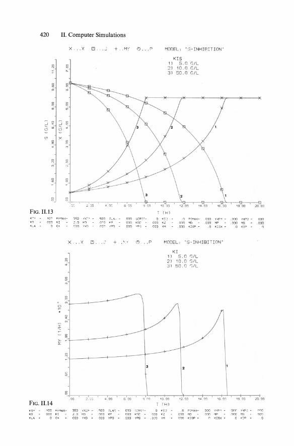
5. Monod kinetics with kd and m. as a combination of Equs. II.7 and II.8. 6. Monod kinetics with S inhibition (cf. Sect. 5.3.5.1). Thus, taking Equs. II.2

and II.3 with Equ. 5.88:

1 Jl(s) = Jlmax 1 + Ks/s + s/K,s

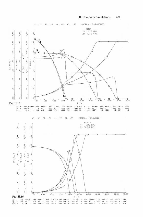
and K,s being the key parameter. 7. Monod kinetics with double substrate limitation (cf. Sect. 5.5):

rx = Jl(S1' t)x + Jl(S2)X' f 1

-rS1 = --' Jl(S1, t)x YX1S1

1 - rS2 = --' Jl(S2)X . f

YX1S2

(11.9)

(11.10)

(II. 11)

(II. 12)

with Equ. II.6 for Jl(S1' t) and the following expression for the term f (cf. Equ. 5.106 or Equ. 5.152):

(II. 13)

with KR being the key parameter for repression and s1,crit representing the substrate concentration, where both substrates are utilized simultane­ously, thus losing the diauxic behavior.

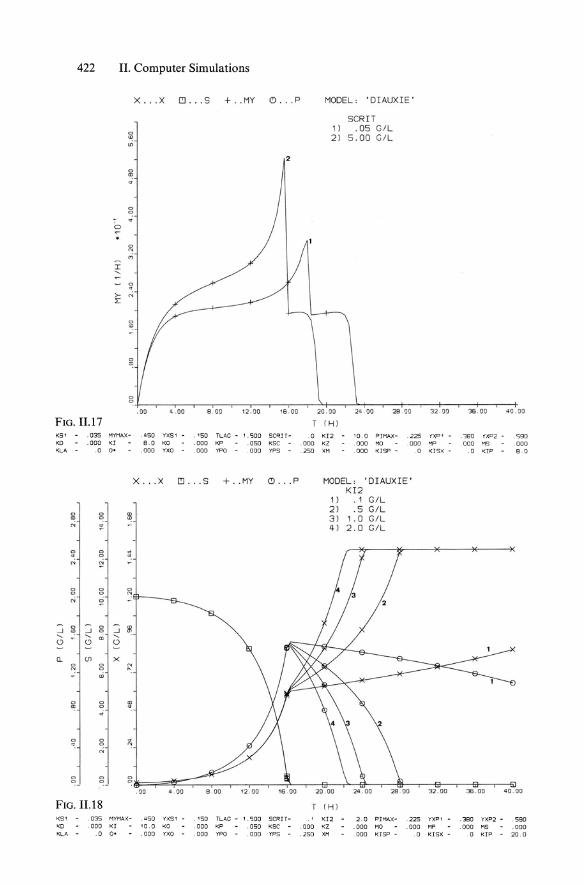
8. Diauxic growth as an analogy to case 7:

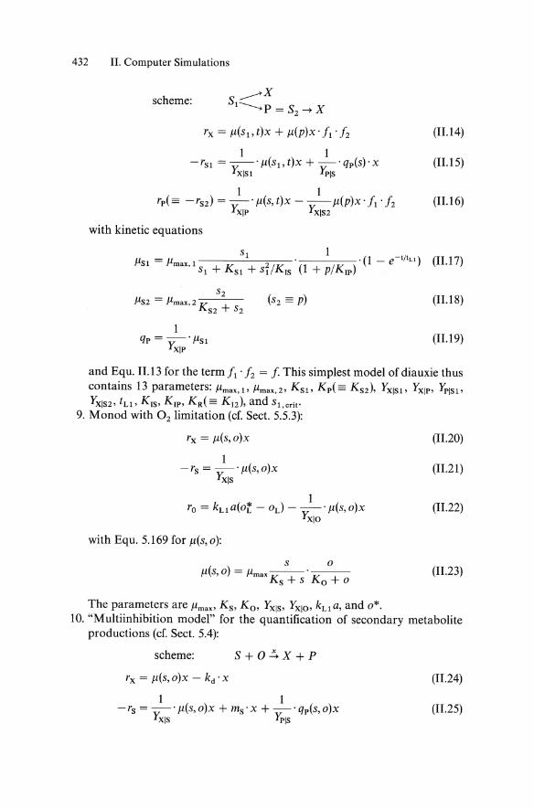
432 II. Computer Simulations

scheme: s.------"X 1------. P = S2 --+ X

rX = fl(Sl,t)X + fl(p)x'f1'f2 (II.14)

1 1 -rS1 = --' fl(Sl' t)x + -' qp(s)' X

YX1S1 YPls (11.15)

(11.16)

with kinetic equations

flS2 = J1m.x, 2 K + S2 S2

S2 (S2 == p) (II.I8)

(II.I9)

and Equ. II.I3 for the term fl' f2 = f This simplest model of diauxie thus contains 13 parameters: flm.x,l, J1max,2, K S1 ' Kp(== K S2 )' YXIS1 ' YxIP ' YPIS1 '

YXIS2 ' t Ll , K ls , KIP, KR (== K12 ), and sl,crit·

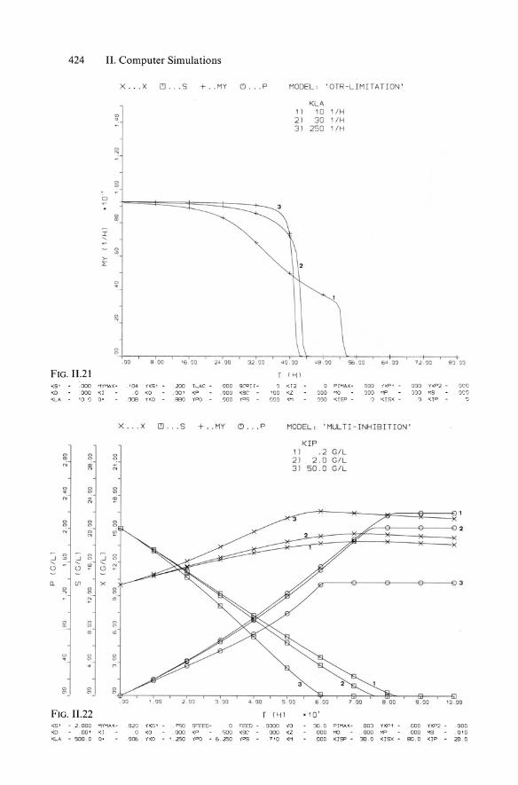
9. Monod with O2 limitation (cf. Sect. 5.5.3):

rX = fl(S,O)X

1 -rs =-'J1(s,o)x

Yxis

with Equ. 5.169 for J1(s, 0):

S ° fl(S,O) = J1m.x Ks + S Ko + °

The parameters are flm.x, K s, Ko, Yx1s, Yx1o , kLl a, and 0*.

(II.20)

(II.21)

(11.22)

(II.23)

10. "Multiinhibition model" for the quantification of secondary metabolite productions (cr. Sect. 5.4):

scheme: S + 0 ~ X + p

rX = fl(S,O)X - kd . x (II.24)

1 1 -rs = -' fl(S,O)X + ms' x + -' qp(s,o)x

YxlS YPls (11.25)

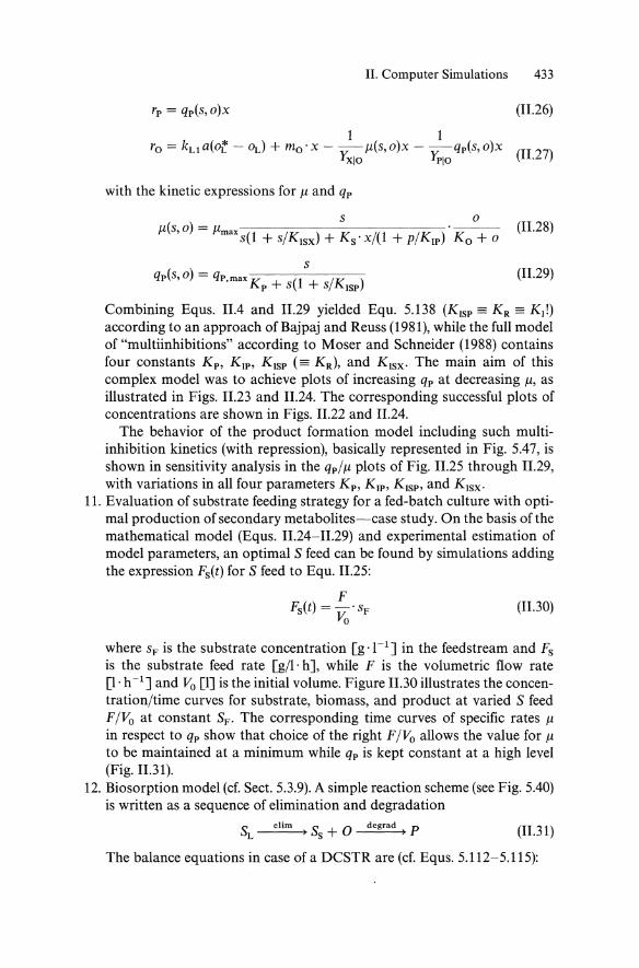
II. Computer Simulations 433

rp = qp(s,o)x (11.26)

ro = kLl a(or - ~) + rno' x - _1_Jl(s, o)x - _1_qp(s, o)x (11.27) Yxlo lPlo

with the kinetic expressions for Jl and qp

s 0

Jl(s, 0) = Jlmax s(1 + s/KISX) + K S'x/(1 + p/KIP) Ko + 0 (11.28)

s qp(s,o) = qP,max Kp + s(1 + s/KISP) (11.29)

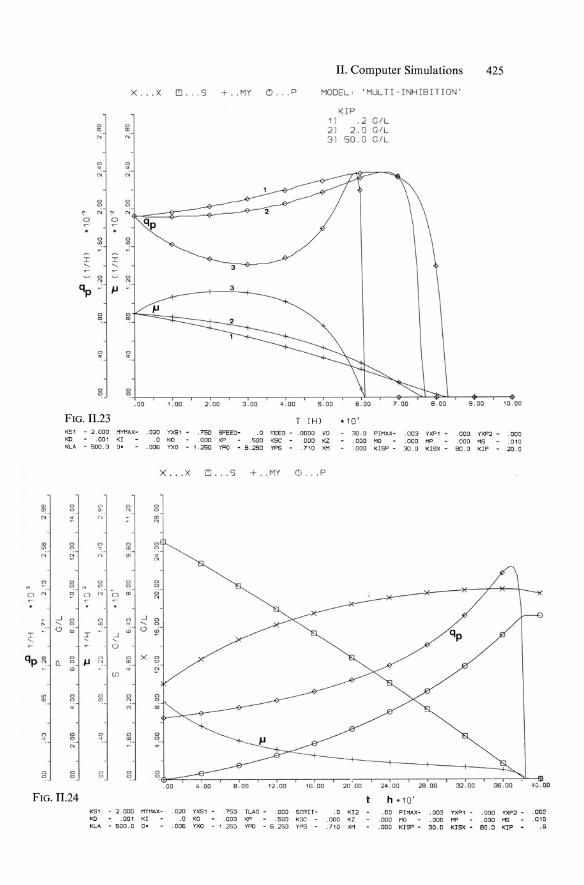
Combining Equs. 11.4 and 11.29 yielded Equ. 5.138 (KISP == KR == KI!) according to an approach of Bajpaj and Reuss (1981), while the full model of "multiinhibitions" according to Moser and Schneider (1988) contains four constants Kp, KIP, Kisp (== KR), and Klsx ' The main aim of this complex model was to achieve plots of increasing qp at decreasing Jl, as illustrated in Figs. 11.23 and 11.24. The corresponding successful plots of concentrations are shown in Figs. 11.22 and 11.24.

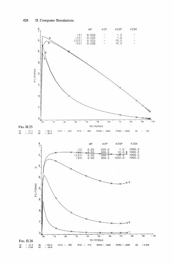
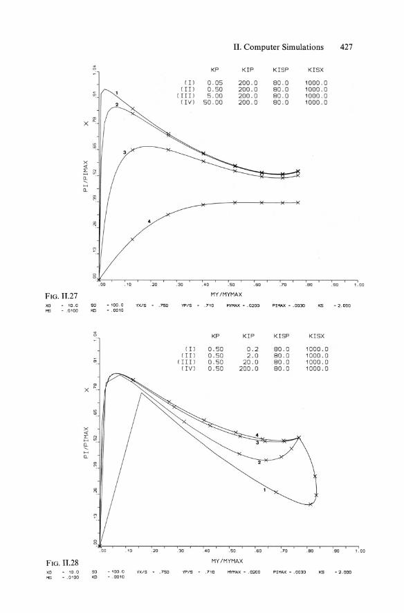
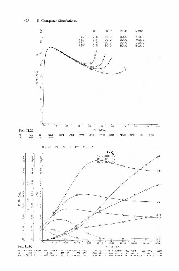
The behavior of the product formation model including such multi­inhibition kinetics (with repression), basically represented in Fig. 5.47, is shown in sensitivity analysis in the qp/Jl plots of Fig. 11.25 through 11.29, with variations in all four parameters Kp, KIP' KISP' and KISX'

11. Evaluation of substrate feeding strategy for a fed-batch culture with opti­mal production of secondary metabolites-case study. On the basis of the mathematical model (Equs. 11.24-11.29) and experimental estimation of model parameters, an optimal S feed can be found by simulations adding the expression Fs(t) for S feed to Equ. 11.25:

F Fs(t) = -'SF

Vo (11.30)

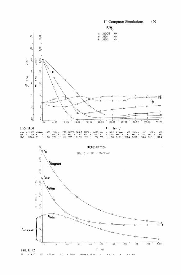
where SF is the substrate concentration [g ,1-1 ] in the feedstream and Fs is the substrate feed rate [gil' h], while F is the volumetric flow rate [1. h -1] and Vo [1] is the initial volume. Figure 11.30 illustrates the concen­tration/time curves for substrate, biomass, and product at varied S feed F /Vo at constant SF' The corresponding time curves of specific rates Jl in respect to qp show that choice of the right F /Vo allows the value for Jl to be maintained at a minimum while qp is kept constant at a high level (Fig. 11.31).

12. Biosorption model (cf. Sect. 5.3.9). A simple reaction scheme (see Fig. 5.40) is written as a sequence of elimination and degradation

SL elim) Ss + 0 degrad) p (11.31)

The balance equations in case of a DCSTR are (cf. Equs. 5.112-5.115):

434 II. Computer Simulations

(II.32)

(II.33)

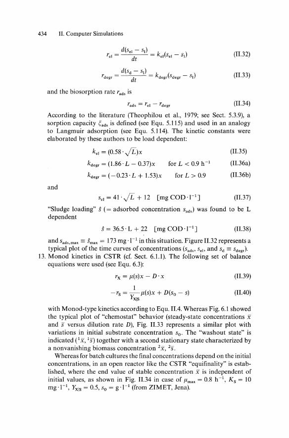
and the biosorption rate rads is

(II.34)

According to the literature (Theophilou et ai., 1979; see Sect. 5.3.9), a sorption capacity ~ads is defined (see Equ. 5.115) and used in an analogy to Langmuir adsorption (see Equ. 5.114). The kinetic constants were elaborated by these authors to be load dependent:

ke• = (0.58' fi)x kdegr = (1.86' L - 0.37)x for L < 0.9 h-1

kdegr = (-0.23' L + 1.53)x for L > 0.9

and

Se. = 41· fi + 12 [mg COD '1-1 ]

(11.35)

(11.36a)

(1I.36b)

(II.37)

"Sludge loading" s (= adsorbed concentration Sads) was found to be L dependent

s = 36.5' L + 22 [mg COD '1-1 ] (11.38)

and sads,max == smax = 173 mg .1-1 in this situation. Figure 11.32 represents a typical plot of the time curves of concentrations (Sad., Se., and Sd == Sdegr)'

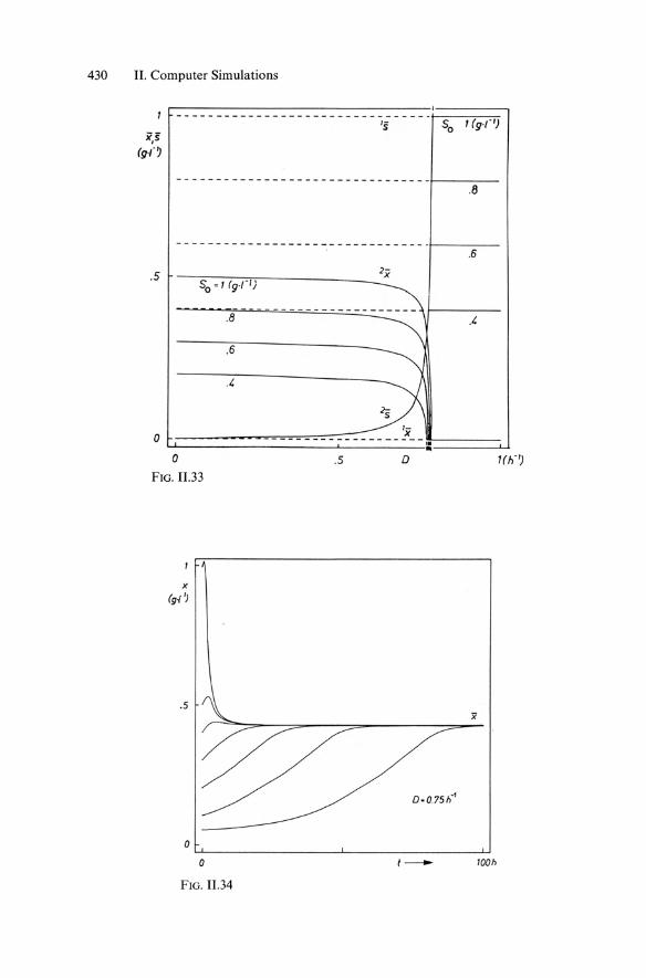
13. Monod kinetics in CSTR (cf. Sect. 6.1.1). The following set of balance equations were used (see Equ. 6.3):

rx = jl(s)x - D . x

1 - rs = y,- jl(s)x + D(so - s)

xis

(II.39)

(II.40)

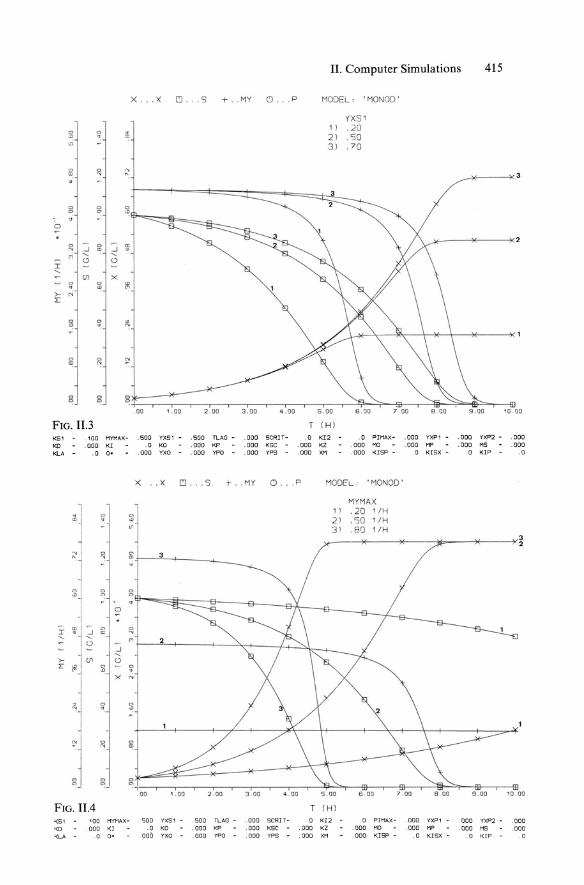
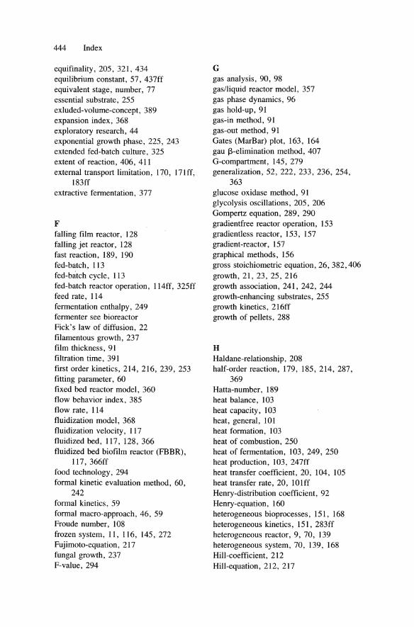
with Monod-type kinetics according to Equ. 11.4. Whereas Fig. 6.1 showed the typical plot of "chemostat" behavior (steady-state concentrations x and "8 versus dilution rate D), Fig. 11.33 represents a similar plot with variations in initial substrate concentration So. The "washout state" is indicated (1 x, 1"8) together with a second stationary state characterized by a nonvanishing biomass concentration 2 X, 2"8.

Whereas for batch cultures the final concentrations depend on the initial concentrations, in an open reactor like the CSTR "equifinality" is estab­lished, where the end value of stable concentration x is independent of initial values, as shown in Fig. 11.34 in case of jlmax = 0.8 h-1, Ks = 10 mg '1-1, YxlS = 0.5, So = g .1-1 (from ZIMET, Jena).

II. Computer Simulations 435

CSTR behavior in case of more complex kinetics has been shown in Figs. 6.4 through 6.11 and 6.14 through 6.20. Alternative bioreactor opera­tions (CPFR, NCSTR, RR, etc.) were represented in Sects. 6.4 through 6.8.

BIBLIOGRAPHY

General: Ropke, H., Riemann, J. (1969). Analogcomputer in Chemie und Biologie, Berlin:

Springer-Verlag. Knorre, W.A. (1971). Analogcomputer in Biologie und Medizin. Jena: VEB G. Fischer. Romanovsky, J.M., Stepanova, N.V., and Chernavsky, D.D. (1974). Kinetische

Modelle in der Biophysik. Jena: VEB G. Fischer. Levin, S. (ed.) (1981). Modeles Mathematiques en Biologie, Berlin: Springer-Verlag. Knorre, W.A. (1980). Kinetische Modelle in der Mikrobiologie in "Biophysikalische

Grundlagen der Medizin (Beier W., Rosen R., eds.) Stuttgart: Fischer. Spain, J.D. (1984). Basic Microcomputer Models in Biology, Addison-Wesley Pub!.

Comp., Reading, Massachusetts, USA. Rogers, P.L. (1976). In Advances Biochem. Engng. 4,125.

Special: Bajpaj, R.K., Reuss M. (1981). Biotechnol. Bioengng., 23, 717. Moser, A., Schneider, H. (1988). Bioprocess Engineering 3, in press. Theophilou, J., Wolgbauer, 0., and Moser, F. (1979). Gas-Wasser-Fach-Wasser/

Abwasser 120, 119.

APPENDIX III

Microkinetics: Derivation of Kinetic Rate Equations from Mechanisms

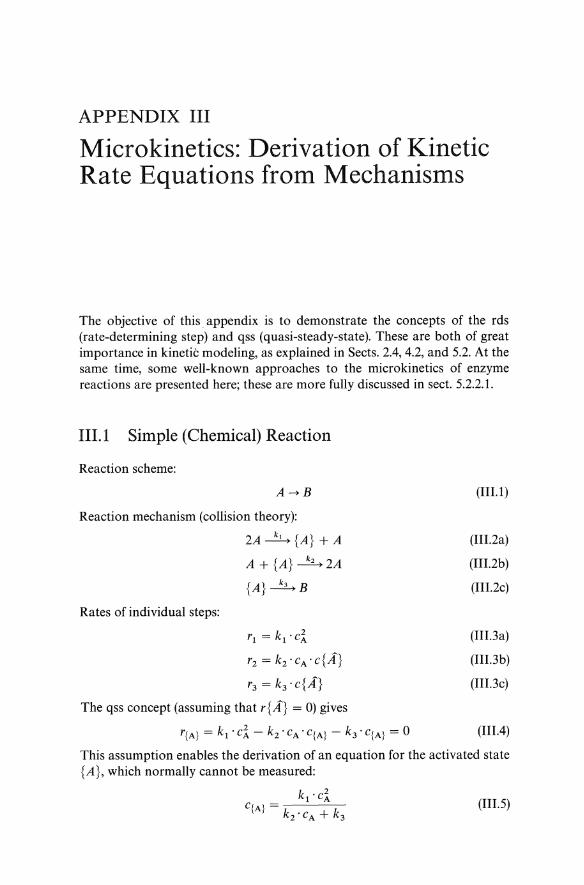
The objective of this appendix is to demonstrate the concepts of the rds (rate-determining step) and qss (quasi-steady-state). These are both of great importance in kinetic modeling, as explained in Sects. 204, 4.2, and 5.2. At the same time, some well-known approaches to the microkinetics of enzyme reactions are presented here; these are more fully discussed in sect. 5.2.2.1.

IlL 1 Simple (Chemical) Reaction

Reaction scheme:

Reaction mechanism (collision theory):

2A~{A} +A

A + {A}~2A {A}~B

Rates of individual steps:

r1 = kl ·d. r2 = k2 ·cA ·c{A}

r3 = k3 ·c{A}

The qss concept (assuming that r{A} = 0) gives

(1II.1 )

(III.2a)

(HI.2b)

(HI.2c)

(II I.3 a)

(lII.3b)

(II I.3 c)

riA} = kl . c1 - k2 . CA . CIA} - k3 . CIA} = 0 (lIlA)

This assumption enables the derivation of an equation for the activated state {A}, which normally cannot be measured:

(111.5)

111.3 Briggs-Haldane Approach 437

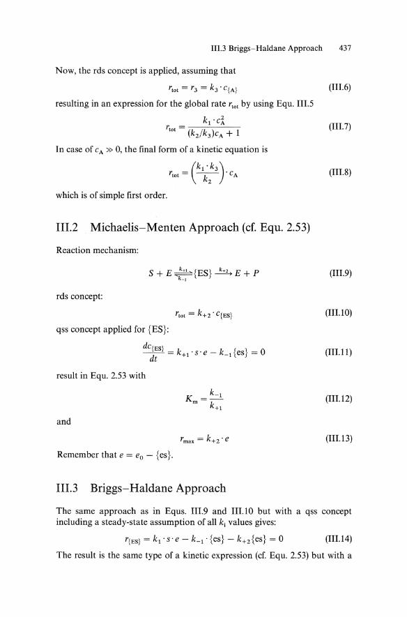
Now, the rds concept is applied, assuming that

rtot = r3 = k3 . C{A} (III.6)

resulting in an expression for the global rate rtot by using Equ. III.5

kl ·ci rt t = (III. 7)

o (k2/k3)CA + 1

In case of CA » 0, the final form of a kinetic equation is

which is of simple first order.

III. 2 Michaelis-Menten Approach (cf. Equ. 2.53)

Reaction mechanism:

S+E~{ES}~E+P k_1

rds concept:

qss concept applied for {ES}:

dC(ES} dt = k+1's'e - Ldes} = 0

result in Equ. 2.53 with

and

Remember that e = eo - {es}.

III. 3 Briggs-Haldane Approach

(III.S)

(III.9)

(III.10)

(II1.ll)

(III.12)

(III.13)

The same approach as in Equs. III.9 and III.10 but with a qss concept including a steady-state assumption of all k i values gives:

(II1.l4)

The result is the same type of a kinetic expression (cf. Equ. 2.53) but with a

438 III. Microkinetics: Derivation of Kinetic Rate Equations from Mechanisms

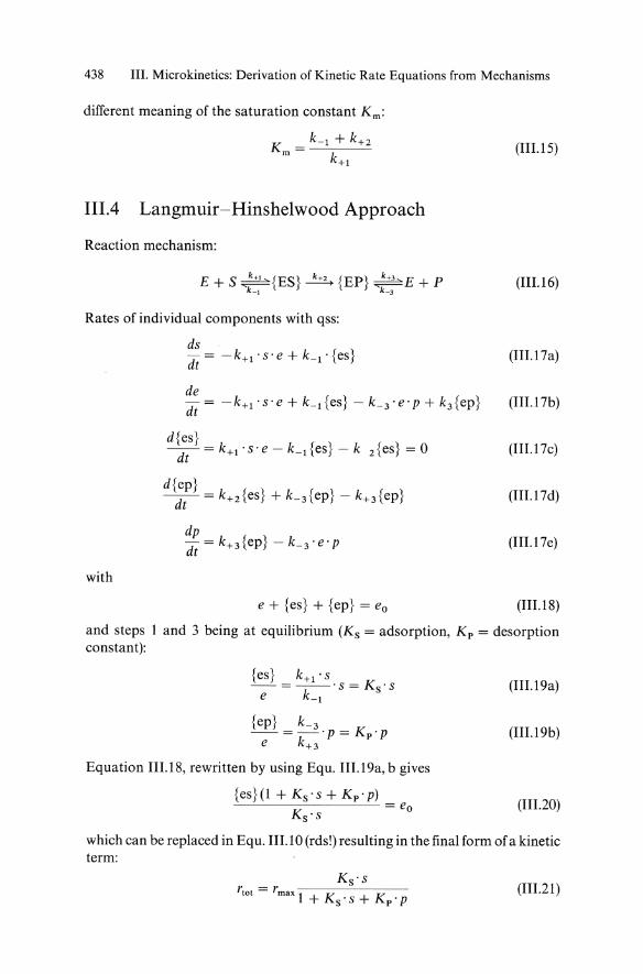
different meaning of the saturation constant Km:

Ll + k+2 K = ---c---m k+1

IlIA Langmuir-Hinshelwood Approach

Reaction mechanism:

E + s ~{ES} ~ {EP} ':"=:-E + P k~ k~

Rates of individual components with qss:

ds dt = -k+l ·s·e + L 1 · {es}

de dt = -k+l ·s·e + Ll {es} - L3 ·e· p + k3{ep}

d{ es} --;[t = k+l . s· e - Lr{es} - k 2{es} = 0

d{ep} ----;[t" = k+2{es} + L3{ep} - k+3{ep}

dp dt =k+3{ep} -L3 ·e·p

with

e + {es} + {ep} = eo

(IILI5)

(IILl6)

(III.17a)

(I1I.l7b)

(111.17c)

(III.17d)

(III.17e)

(IILl8)

and steps 1 and 3 being at equilibrium (Ks = adsorption, Kp = desorption constant):

{ep} L3 --=-·p=Kp·p

e k+3

Equation 111.18, rewritten by using Equ. IILl9a, b gives

{es}(l + Ks·s + Kp· p) = eo

Ks·s

(III.19a)

(III.l9b)

(III. 20)

which can be replaced in Equ. IILl 0 (rds!) resulting in the final form of a kinetic term:

Ks·s r = r

tot max 1 + K s . s + K p . P (Hl.2l)

III.6 Reversible Langmuir-Hinshelwood Approach 439

This is the general form of the Langrnuir-Hinshelwood equation applicable to heterogeneous chemical catalysis.

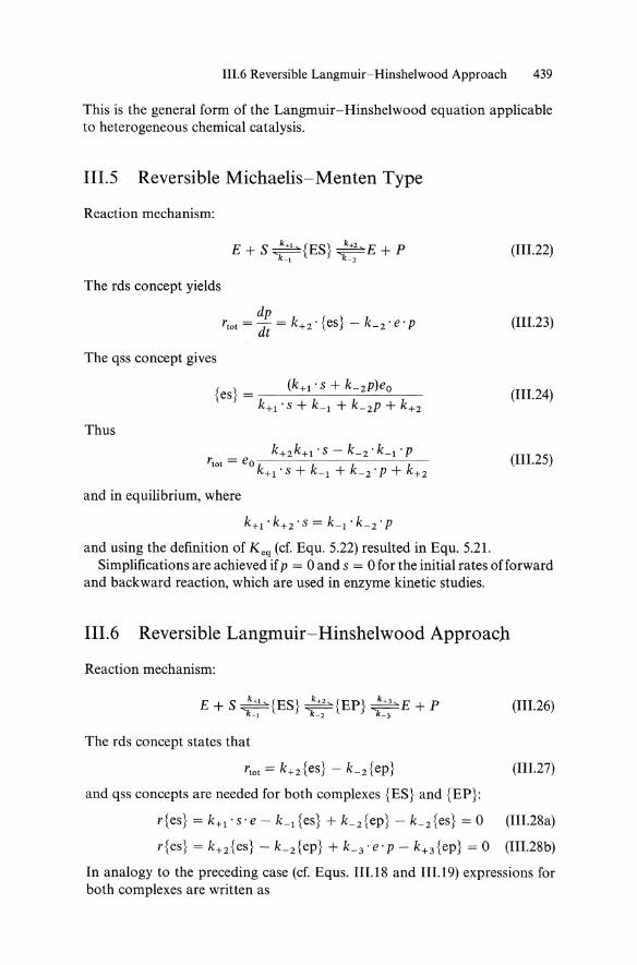
IlL5 Reversible Michaelis-Menten Type

Reaction mechanism:

E+S~{ES}~E+P k-, k-2

(111.22)

The rds concept yields

dp rtot = dt = k+2·{es} - k_2·e·p (111.23)

The qss concept gives

{ } (k+l . S + L2p)eO es = -----''----'''---=----

k+l . S + Ll + L 2P + k+2 (111.24)

Thus

(111.25)

and in equilibrium, where

k+l . k+2 . S = Ll . L2 . P

and using the definition of Keq (cf. Equ. 5.22) resulted in Equ. 5.21. Simplifications are achieved if P = 0 and s = 0 for the initial rates of forward

and backward reaction, which are used in enzyme kinetic studies.

IlL6 Reversible Langmuir-Hinshelwood Approach

Reaction mechanism:

E + s ~{ES} 2±.h{EP} ~E + P k_, ~ ~

(III.26)

The rds concept states that

rtot = k+2{es} - L2{ep} (III.27)

and qss concepts are needed for both complexes {ES} and {EP}:

r{es} = k+l -s-e - Ll res} + L2{ep} - L2{es} = 0 (III.28a)

r{es} = k+2{es} - L2{ep} + k-3 ·e· p - k+3{ep} = 0 (III.28b)

In analogy to the preceding case (cf. Equs. 111.18 and II1.19) expressions for both complexes are written as

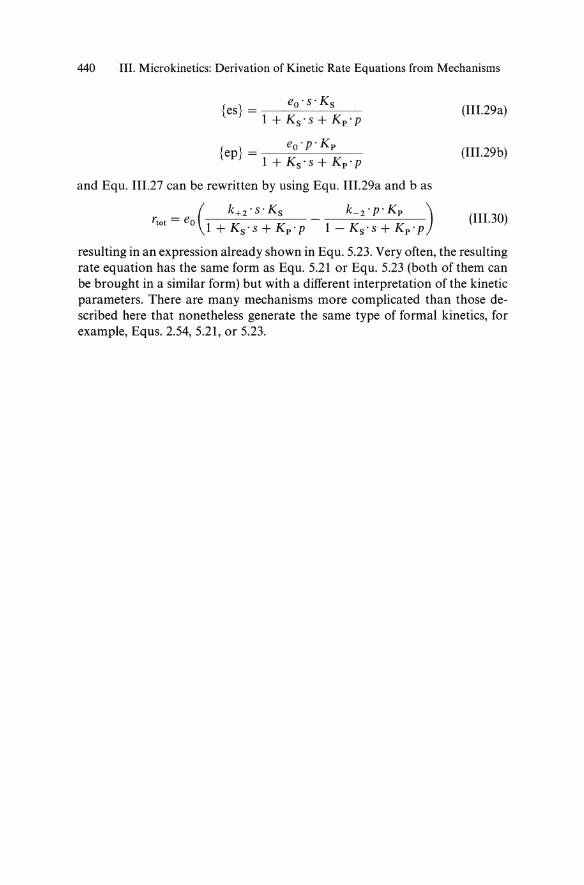
440 III. Microkinetics: Derivation of Kinetic Rate Equations from Mechanisms

eo ·s· Ks {es} - ----'----"--

1+Ks's+Kp 'p

eO'p'Kp {ep} - ---=--=---=--

1+Ks's+Kp 'p

and Equ. III.27 can be rewritten by using Equ. III.29a and b as

( k+2'S'Ks L 2'P'Kp ) rtot = eo -

1+Ks's+Kp 'p 1-Ks's+Kp 'p

(III.29a)

(III.29b)

(III.30)

resulting in an expression already shown in Equ. 5.23. Very often, the resulting rate equation has the sameJorm as Equ. 5.21 or Equ. 5.23 (both of them can be brought in a similar form) but with a different interpretation of the kinetic parameters. There are many mechanisms more complicated than those de­scribed here that nonetheless generate the same type of formal kinetics, for example, Equs. 2.54, 5.21, or 5.23.

Index

A absolute deviation, 89 absolute rate, 19,20 absorption, 221 activated state, 203, 436ff activation, 199 activation energy, 199, 200 activity function of product formation,

276 adaptation constant, 277 adaptational parameter, 60 adaptive modeling, 50 adsorption, 240 aeration number, 106 age, 246 allosteric control, 217 allosteric inhibition, 232 allosterie, 212, 217 amensalism, 261, 265 anhydrase-method, 190 apical growth, 238 apparent morphology, 390 apparent rate, 172 apparent value, 172 apparent viscosity, 387 Arrhenius equation, 199 Arrhenius plot, 200, 201 assimilation, 220, 221 Atkinson equation, 283 ATP, 29, 30, 245, 282 attraction domains, 320 autocatalytic process, 344, 345 autocatalysis, 25 autoregulation, 205 available electrones, 31 axial dispersion, 122, 175

B Back mix-plug flow model, 84 balance, mass, 118ff balanced growth, 145, 157, 272 balanced system, 11, 116, 145, 272 balancing method, 53, 382ff batch reactor see discontinuous reactor bed expansion, 117 bed porosity, 369 bench scale (lab scale), 44 Bingham plastic, 385 biocoenosis, 10, 259, 260, 293 biodisc reactor, 68, 139 biofilm,68 biofilm kinetics, 151, 283ff biofilm operation, 69, 139 biofilm reactor operation, 69, 139, 358ff biological inertia, 198, 212, 214 biological rate equation, 178, 283f biological test system, 41, 87, 90, IlOff biomass, 19 biomass holdup, 367 bioparticle terminal Re number, 369 Bioprocess design, 307ff Bioprocess kinetics, 19, 197ff Bioprocess technology, 5, 7, 13 bioreactor, 2, 66ff, 73, 307 bioreactor concept, 112 bioreactor dimensioning, 127 bioreactor model, 44, 45, 56, 112, 118ff,

125,307 bioreactor operation, 112, 307 bioreactor performance, 307ff biosociety, 1 biosorption, 238, 342 biosorption model, 238, 433

442 Index

biosorption rate, 434 biotechnology, 1 Biot-number, 187 bistable system, 319 bistability, 319, 320 blads box model, 48 Blackman-kinetic, 218 bleed stream, 378 BOD, 292 BODs, 292 BODpu 292 Bodenstein-number, 75, 80, 86,

347 Boltzmann-constant, 203 bottleneck, 206, 436ff, 218 boundaries (closed, open), 76 boundary conditions, 76, 169, 176 branching rate, 238 Briggs-Haldane approach, 437 Briggs-Haldane equation, 208, 437 bubble column, 67 bulk, 18, 168

C calculation methods, 349ff calorimetry, 104 Carbon-flow-brenching concept, 37 Carman-factor, 147 cascade, 77, 113, 333, 353 cascade of reactors with cell recycling,

353 Casson equation, 386, 389 Casson viscosity, 386 catabolite repression, 145, 251, 237 catalytic constant, 234 catalytic process, 344 cell age, 246 cell age (mean), 246 cell cycle, 379 cell model, 58, 77 cell tissue culture, 67 characteristic diameter, 105 characteristic length, 75 characteristic times, 142, 393 characteristic-time concept, 14lff chemostat, 119 circulation time distribution, 88 circulation time, 82, 86, 89, 90 closed boundaries, 76 closed environment, 261

closed environment, 261 C-mole (of biomass), 28 COD, 292 community matrix, 261 commensalism, 261, 265 compartment 279, 144, 145 compensation, 203 competition, 261, 262f competitive inhibition, 209 completely mixed microbial film fermen-

ter, 128 complex reaction system, 406 computer simulation, 412ff COiNaOH-method, 190 concentration polarization, 373 concept of characteristic times, 14lff conductivity, 81, 93 conservation of mass, 22 consistency index, 387 constant of adaptation, 277 constant growth phase, 219, 244 constant-volume continuous stirred tank

reactor, 119 constant volume reactor operation, 113,

119 consumption activity coefficient, 243 continuous mode of reactor operation, 10,

113 continuous recycle reactor, 123, 351 continuous plug flow reactor (CPFR),

113, 121, 337ff continuous stirred tank reactor (CSTR),

113, 119, 308ff, 434 Contois-kinetics, 217 controlled filmthickness, 126, 138 convection coefficient, 91 convection theory, 91 conversion, 38 costs, 40 critical diameter, 147, 150, 177 critical film thickness, 147, 150, 177 critical S-concentration, 252 critical treshold concentration, 233 critical washout point, 309 cross-inhibition, 255 crowding factor, 391 CTR control, 309 cube root equation, 289 cycle time distribution, 87, 88 cyclic operation, 116, 325

D Damkoehler-number-l" degree, 347 Damkoehler-number-2nd degree, 148,

176, 185 damped oscillations, 270 Danckwerts boundry conditions, 169 Danckwerts reactor, 129, 191 death, microbial, 227 death, phase, 225 death rate constant, 227, 228, 230 decay rate (decomposition), 244 decimal reduction time, 202 declining growth phase, 243 deduction, 10 deductive method, 50 definition of reaction rate, 23ff, 155 degradation (substrate), 221, 239,240 degree of Hinterland, 99 degree of (micro) mixing, 81 degree of 02-utilization, 99 degree of reductance, 32 degree of reduction, 32 degree of segregation, 72, 83, 349, 350 depth of penetration, 179 deviation variables, 275 dialysis (membrane) reactor operation,

371 dialysis reactor, 371 diauxic growth, 237, 251, 431 diauxie, 226 differential analysis, 11, 156 differential evaluation method, 154 differential reactor, 11, 152 diffuson, 22, 75, 91 diffusion regime, control, 171, 177, 185,

189 dilution rate, 119 "direct linear" plot, 167 discontinous mode of reactor operation,

113,119 discontinuous recycle reactor, 123 discontinuous stirred tank reactor, 119 dispersion (coeff.), 75, 122 dispersion model, 74, 122 dissipation (energy), 147, 181 distributed parameter reactor, 121, 113,

151 Dixon-plot, 211 double-substrate-Iimitation function, 255ff D-value, 294

Index 443

DIO value, 202, 294 dynamic flow eqUilibrium, 204 dynamic method, 90, 92, 94, 102 dynamic models, 95, 272ff dynamic process (kinetics), 274ff dynamics of enzyme synthesis, 213

E Eadie-Hofstee plot, 166, 174, 180 economy (of °2), 10 I economics, 38 effective hyphal length, 238 effectiveness factor, 11, 148, 170, 182,

186, 286 effectiveness, GIL, 148 effectiveness, intraparticle, 148 effectiveness, liquid/particle, 149 effectiveness, surface based, 182 effectiveness, volume based, 170, 178 effective rate, 170, 173, 177, 179, 180,

185 effectivity, 170 efficiency general, 11, 47 efficiency of motor, 100 efficiency of °2 , 101 electrode dynamics, 97 electrode response, 97 elementary analysis, 25, 382, 406 element balance, 382 element-species matrix, 407 elimination, 221, 239, 240 elutriation, 117 empiric pragmatic approach, 11, 16 endogeneous metabolism, 198,216,

228ff energy dissipation, 147, 181 energy efficiency coefficient, 31 energy of activation, 199 engineering morphology, 390 enhancement factor, 170, 189 enhancement of transport, 170, 188ff enhancing substrate, 255 enthalpy, 203 enthalpylentropy compensation, 203 entropy, 203 enzyme kinetics, 436ff enzyme mechanisms, 436ff enzyme reactor, 68, 311, 338, 341, 344 enzyme regulation and control, 211

444 Index

equifinality, 205, 321, 434 equilibrium constant, 57, 437ff equivalent stage, number, 77 essential substrate, 255 exluded-volume-concept, 389 expansion index, 368 exploratory research, 44 exponential growth phase, 225, 243 extended fed-batch culture, 325 extent of reaction, 406, 411 external transport limitation, 170, 171ff,

183ff extractive fermentation, 377

F falling film reactor, 128 falling jet reactor, 128 fast reaction, 189, 190 fed-batch, 113 fed-batch cycle, 113 fed-batch reactor operation, 114ff, 325ff feed rate, 114 fermentation enthalpy, 249 fermenter see bioreactor Fick's law of diffusion, 22 filamentous growth, 237 film thickness, 91 filtration time, 391 first order kinetics, 214, 216, 239, 253 fitting parameter, 60 fixed bed reactor model, 360 flow behavior index, 385 flow rate, 114 fluidization model, 368 fluidization velocity, 117 fluidized bed, 117, 128,366 fluidized bed biofilm reactor (FBBR),

117, 366[f food technology, 294 formal kinetic evaluation method, 60,

242 formal kinetics, 59 formal macro-approach, 46, 59 Froude number, 108 frozen system, II, 116, 145,272 Fujimoto-equation, 217 fungal growth, 237 F-value, 294

G gas analysis, 90, 98 gas/liquid reactor model, 357 gas phase dynamics, 96 gas hold-up, 91 gas-in method, 91 gas-out method, 91 Gates (MarBar) plot, 163, 164 gau f3-elimination method, 407 G-compartment, 145, 279 generalization, 52, 222, 233, 236, 254,

363 glucose oxidase method, 91 glycolysis oscillations, 205, 206 Gompertz equation, 289, 290 gradientfree reactor operation, 153 gradientless reactor, 153, 157 gradient-reactor, 157 graphical methods, 156 gross stoichiometric equation, 26, 382,406 growth, 21, 23, 25, 216 growth association, 241, 242, 244 growth-enhancing substrates, 255 growth kinetics, 216ff growth of pellets, 288

H Haldane-relationship, 208 half-order reaction, 179, 185,214,287,

369 Hatta-number, 189 heat balance, 103 heat capacity, 103 heat, general, 101 heat formation, 103 heat of combustion, 250 heat of fermentation, 103, 249, 250 heat production, 103, 247ff heat transfer coefficient, 20, 104, 105 heat transfer rate, 20, 101ff Henry-distribution coefficient, 92 Henry-equation, 160 heterogeneous bioprocesses, 151, 168 heterogeneous kinetics, 151, 283 ff heterogeneous reactor, 9, 70, 139 heterogeneous system, 70, 139, 168 HilI-coefficient, 212 Hill-equation, 212, 217

HiII-kinetics, 212 HiII-plot, 213 Hinshelwood's network theory, 238 hinterland, 99, 189, 190, 358 homeostasis, 261 homogeneous kinetics, 151,216 homogeneous rate equations, 151, 216ff homogeneous reactor, 9, 70 homogeneous system, 70 horizontal position of reactor, 126 hyperbolic type, 212 hyphal growth unit, 239

I ideal single-stage reactor, see CSTR idiophase, 378 inactivation of spores, 294 incomplete mixing, 313 incomplete substrate penetration, 179 induction, 145, 213 induction phase, 243 inductive method, 50 ingestion, 220 inhibition, 145, 198, 209, 233, 252, 255,

339 inhibition types, 209, 210, 233, 234 inhibitor, 209 inhomogeneity, 72, 82, 83 initial rate, 208 integral analysis, 11, 154, 156 integral evaluation method, 155 integral reactor, 11, 151, 338 integrated bioreactor system, 68 integrating strategy, 41ff, 53, 38lff, 396 interactions, 43,61, 140,261,385 interactive model, 256, 257 internal transport limitation, 170, 175ff,

183ff intrinsic rejection, 373 intrinsic viscosity, 392 ionic strength, 93, 232 invariance, 215 isokinetic temperature, 203

J jeopardy, to put a model in, 52 joint analysis, 93, 167

K K-compartment, 145 key reaction, 279, 409 key variable, 26, 408 kinetic model, 54ff

Index 445

kinetic modeling of lag-phases, 225, 430 kinetic modeling of endogenous metabo-

lism, 227, 431 kinetic regime, control, 171, 177, 189,

190 kinetic similarity, 45 KLa-value, 94, 106 Kolmogoroff-theory, 147, 181 Konak-equation,222 Kono approach, 219 Kono concept, 219 Kono-kinetics, 219 Kozeny-Carmen equation, 391

L lag-phase (growth), 145, 216, 225 lag-time, 145, 214, 216, 225, 275 Langmuir-Hinshelwood approach (revers-

ible), 208, 439 Langmuir-Hinshelwood kinetic (irreversi­

ble), 208, 438 Langmuir-kinetics, 57, 160, 165, 166,

240 Langmuir plot, 166, 181 level of sterility, 293 limitation-substrate, 16, 18 limitation-transport, 170 limit cycle (oscillation), 269 limiting viscosity number, 392 Lineweaver-Burk plot, 166, 180, 209 linear dependence, 26, 409 linear growth, 290, 376 linearization, diagram, 159, 16lff linearly independent stoichiometric equa-

tion, 409 lineary independent equations, 409 local isotropic turbulence, 147 logarithmic mean value, 98, 103 logistic equation (low), 226 log-mean value, 98, 103 longitudinal dispersion, 122 Lotka-Volterra analysis, 268 Lotka-Volterra model, 269

446 Index

Lotka-Volterra relationship, 220, 269 lumped parameter reactor, 119, 151 lysis, 312

M macrobalances, 25, 54 macrokinetics, 45, 56, 139 macromixing, 74, 350 macroscopic principle, 18,46, 382 macroscopic yield, 28 Maillard reaction, 295 maintenance coefficient, 229, 230, 282,

312 Malthus type, 224 mass-action law, 143, 2r1 mass balance, 118ff mass flux, 22, 373 mass loading rate per unit biomass

(sludge), 275 mass transfer, 20, 169 mass transport with simultaneous reac-

tion, 169 master reaction, II, 206, 218, 436ff mathematical model, 49, 168 mathematical modeling, 48, 49 matrix, 407 matrix of the stoichiometri coefficients,

407 maturation time, 246, 346 maximum mixedness, 71 mean diameter, 91, 181, 182 mechanism, 55 mechanistic kinetics, 55 mechanistic model, 55, 58 medium design (optimization), 16 membrane performance, 372 membrane permeability, 372 membrane reactor, 371 metabolic process enthalpies, 249 metabolite repression, 145, 252, 237, 389 methodology, 13, 385 Michaelis-Menten approach, 437 Michaelis-Menten equation, 56, 208, 437 Michaelis-Menten kinetics, 56, 160, 437 Michaelis-Menten kinetics (reversible),

208,439 Michaelis-Menten mechanism, 437 Michaelis-Menten model, 437

Michaelis-Menten type (irreversible), 208 microbalances, 25 microbial death phase, 225, 227 microbial interactions, 259 microbial product formation, 240 microfiltration, 371 microkinetics, 45, 55, 204, 436 micromixing, 72, 81, 350 minimal medium, 16 mini lab reactor, 16,44 mixedness, 71 mixed plug flow, 87 mixed population, 259 mixed population kinetics, 259ff mixed substrate kinetics, 250ff mixing, 70, 81 mixing decay rate constant, 88 mixing models, 84 mixing number, 105, 109 mixing time, 81, 83, 89 model, 49 model building, 50, 51, 52 model discrimination, 52 model identification, 50, 52 model parameter, 50 model reactor, 84, 128, 129, 191, 130,

395 modulus, 149, 172, 176, 182, 186, 188 mole of microorganisms, 27 momentum method, 95, 96 Monod equation (kinetics), 56, 160, 166,

216,217,218,224,412 Monod kinetics with death rate, 227,

228,431 Monod kinetics with lag time, 225, 226,

412 Monod kinetics with S-inhibition, 216,

232,431 Monod with O2 limitation, 256, 432 Monod type kinetics with endogeneous

metabolism, 228, 431 monostability, 309 morphology, 389 morphology factor, 389, 390, 391, 392 morphology index, 389 Moser equation (kinetics), 217 multicomponent system, 294 multi inhibition model, 432 multi-loop mixing model, 85

multiple phase bioreactor model, 124 multiple steady states, 265, 267, 321 multi-phase reactor model, 124 multi-purpose reactor, 128 multiresponse analysis, 167 multistage reactor system, 329ff multistage system, 329, 330 multistage system with recycle, 329 multistream multistage operation, 329,

334 multistream system, 329 multisubstrate kinetics, 250ff mutualism, 261, 266f mycelia, 237, 389 mycelial (filamentous) growth, 237, 389

N neutralism, 261 Newtonian fluids, 385 nomenclature, 5, 19,21 noncompetitive inhibition, 209 non-growth-Iinked product formation,

242, 244, 246 noninteractive model, 258 Non-Newtonian fluids, 385 non-stationary kinetics, 272ff non-stationary reactor operation, 411 nonvanishing biomass, 320, 434 non-wash-out state, 320 normal catalytic process, 344 number of equivalent stage, 77 number of tanks in a cascade, 77 numerical fitting, 57, 201, 237

o observed rejection, 373 "on-off' concept, 252 open boundaries, 76 open environment, 261 optimum, biological, 198 optimum conversion, 39, 339, 341, 350 ordinary sinetics, 145 oscillation, 206, 266, 269, 270, 273 OTR control, 309 OUR control, 309 overall transfer coefficient, 186 overlapping (substrate), 252

oxygen economy, 10 1 oxygen efficiency, 101 oxygen saturation, 92 oxygen solubility, 92

Index 447

oxygen transfer number, 106, 109, 110 oxygen transfer rate, 90, 125, 144 oxygen utilization degree, 99 oxystat, 309

p parameter, 50 parameter estimation, 50, 15lff parameter sensitivity analysis, 51, 414ff parasitism, 261 partial dilution rates, 335 Pected number, 75 pellet, 193, 288, 359 penetration, 221 penetration depth, 129, 179 penetration theory, 91 perfect bioreactor, 41, 44, 126ff, 191 performance, 307 performance equations, 307ff peripheral zone model, 289 periodic eqUilibrium curve, 333 periodic reactor operation, 116 period of oscillation permeability, 372, 374 permeate, 373 phased culture techniques, 379 photo bioreactor, 238 photosynthesis, 237 pH-auxostat, 309 pH-dependence (kinetics), 237 pH-stat, 309 phyto technology, 1 pilot plant (reactor), 16, 44 pilot scale, 16, 44 Planck-constant, 203 plug flow reactor, 113, 121, 337f plug flow reactors with recycling, 354 point, 72 polarization, 373 point, 72 Powell kinetics, 217, 287 power consumption, 100 power index, 385 power law constant, 385

448 Index

power law fluid, 385 power number, 105 predation, 261 predator, 268 predator-prey interactions, 268ff preexponential factor, 199 pressure, 10 1 prey, 268 principle of separation, 47 process analysis, 139ff process design, 7, 44 process kinetics, 52, 138 process kinetic analysis, 11, 42, 44,

138ff process parameter, 51 process variable, 19, 52, 60 product formation (kinetics), 240ff, 276f,

314f product formation activity function, 276 product inhibition, 145, 316f product inhibition kinetics, 216, 234ff production of secondary metabolities,

241,244,246,247,278,388,432 productivity, 38, 309, 353 profit, 38 proto cooperation, 266 pseudo-differential reactor, 153 pseudohomogeneity, 11, 146 pseudohomogeneous L-phase reactor

model, 169 pseudohomogeneous rates, 11, 237, 240,

285,360 pseudo-integral reactor, 152 pseudokinetics, 139, 290f pseudokinetic parameters, 173 pseudokinetic phenomena, 173 pumping capacity, 393f, 17

Q Q-value, 276 qe,24 qH,24 qQ, 24, 94, 139, 223 qs,24 quantification, 6, 18,47,73,241 qss (quasi steady state), 11, 42, 120,

157 quasi-steady state reactor operation, 120,

327

R rank of matrix, 407 rate, 20 rate coefficient, 20 rate determining step (rds), 11,42,218 rate of apical growth, 238 rate of branching, 238 rate of permeation, 373 "rds concept", 11, 206, 436ff, 272, 360 reaction enthalpy of fermentation, 249 reaction order, 214 reaction rate definition, 23, 24, 25 reaction time, 92, 146 reactor with gradients, 157 real plug flow reactor, 122 real stat , 119 recycle rate, 79 recycle ratio, 79, 86 recycle reactor operation, 79, 154, 351ff reductance, 32 reductance degree, 32 reduction, 32 reference fermentation, 112 regime analysis, 14lff regulation of enzyme amount, 145, 206ff,

211 regulation of enzyme activity, 145, 206ff,

211 Reith-approximation, 189 relative growth rate, 23, 222 relative rate, 20 relati ve velocity, theory, 147 relaxation time (see characteristic time),

277 relaxed steady state, 116 repeated fed-batch, 114, 325 repression, 145, 213 repression kinetics, 237, 248, 389 residence time distribution, 74, 341 response time, 95, 142 reversed-two-environment model, 84 reverse osmosis, 371 Reynolds-number, 108 rheology, 385 ribosome, 214, 252

S salinity, 223 saturation constant, 56

saturation-type kinetics, 56, 160ff, 198, 217ff

Sauter-diameter, 91, 182 scale-down, 45 scale-up, 17, 381 scale-up concept, 381 scale-up correlation, 107ff Schmidt-number, 108 screening, 14 second order kinetics, 214 secondary metabolite productions, 241,

345,432 segregated kinetic model, 49 segragation, total, 72 selectivity, 38 semibatch culture, 113, 325, 4-10 semicontinuous mode of reactor opera-

tion, 10, 113, 410 semicontinuous stirred tank reactor, 1 13,

119 sensitivity analysis, 51, 53, 414ff separation, 47 sequential S-utilization, 25lff shear rate, Ill, 385, 387 shear stress, 385 Sherwood-number, 108, 174 shift-down, 319, 322, 323 shift-up, 319, 322, 323 sigmoidal type, 212 significant variable, 18 simplification, 46 simultaneous S-utilization, 253ff single cell model, 58 single-stream multistage operation, 331 single-stream reactor operation, 331 sloping plane bioreactor, 126, 128 slow reaction, 171, 189 sludge adsorption, 238 sludge loading, 275 sorption capacity, 240 sorption number, 106, 109, 110 specific growth rate, 23 specific heat capacity specific rate, 20 spores, 293, 295 spouted bed, 117 spouted fluidized bed, 117 spread of distribution, 76 stability analysis, 266, 318 stable oscillations, 269, 270

Index 449

stable steady states, 309, 319, 323 standard bioreactor, 127 stationary method, 98 stationary phase of growth, 225, 226 stationary state, 119, 157, 204, 207 steady state, 119, 157,204,207,320,

380 steady state growth, 157, 273, 274 sterilization process, 346 sterilization kinetics, 292ff sterilization level, 293 sterilization process, 293 sterilizer, 68 stimulation, 198 stoichiometrical coefficients, 34 stoichiometrical dependence, 26 stoichiometric line, 256 stoichiometric matrix, 407 stoichiometry, 11,20,25,34, 382ff,

406ff stoichiometry (balancing methods), 382 stoichiometry of complex reactor opera-

tion,406ff strain gauge, 100 strategy, 15, 396 structured cell model, 58, 145 structured kinetics models, 145, 278ff structured modeling of bioreactors

(OTR), 144, 392 structured models, 82, 87, 144 structured reactor models, 82, 87, 144,

392ff substrate, 145 substrate inhibition, 145 substrate inhibition kinetics, 216, 232ff,

318 substrate-utilization kinetics (sequential),

251 substrate-utilization kinetics (simultane-

ous), 216, 253 sugar-feeding strategies, 433 sulphite oxidation, 189ff sulphite oxidation method, 90, 189ff surface area, 90 surface renewal rate, 91 surface renewal theory, 91 survival of the fittest model, 262 symbiosis, 261 synergism, 261 synchronous culture operation, 378ff

450 Index

synchronous/synchronized pulsed and phased culture, 379

systematic approach, 5, 15, 41

T tanks in series model, 77 Teissier kinetics, 217, 232 temperature, 198 temperature dependence, 198 test of pseudohomogeneity, 146ff test system of biolog. test system theory of activated complexes, 203 thermodynamic efficiency, 31, 32, 33 Thermodynamics, 25 Thiele-modulus, 149, 172, 176, 178,

182, 187, 286 Thiele-modulus based on biofilm thick-

ness, 188 Thiele-modulus for zero-order, 179, 186 Thiele-modulus generalized, 187 Thiele modulus f. 1st order, 178, 187 thin layer (tubular film) fermenter, 126,

128, 129 three-compartment model, 145 three-constant (parameter) equation, 218,

235 threshold concentration, 233 time lags, 97 torque, 100 Toe, 292 total hyphal length, 390 total segregation, 7lf toxic power number, 236 toxicity, 198 trajectory, 264, 321, 320, 323 transient behavior of the CSTR, 157, 321 transient operation, 157 transient reactor operation, 157, 325 transient kinetics, 145, 321 transient state, 207, 321 transient phase, 243 transition line, 257 transport coefficient, overall, 185ff transport coefficient, volumetric, 94 transport enhancement, 140, 170, 188ff transport limitation, 140, 170 transport rate, 19

troprophase, 378 tubular reactor, 67, 69, 238 turbidistat, 309 two-compartment model, 144, 280ff, 394 two-environment model, 84 two-film theory, 91 two-phase reactor model, 357 two-region-mixing model, 84 two-stage reactor, 330 two-zone model, 84, 192 types of kinetic models, 54, 151

U Uhlich approximation, 103 ultrafiltration, 371 unbalanced growth, 157 uncompetitive inhibition, 209 uncontrolled film thickness, 138 unified performance, 364 unsegregated model, 49 unstable state, 319 unsteady state reactor operation, 157 unstructured models, 118, 146, 216 unstructured models (kinetics), 146,

216ff, 274ff unstructured models (reactors), J 18ff

V variable, 52, 60 variable volume reactor operation, 119,

325 variance, 72, 89 Verhulst-equation, 224 Verhulst-Pearl's equation, 224, 225 viscosity, 385 volume-based effectiveness factor, 178,

182 volumetric heat, 18, 20, 103 volume-utilization (see hinterland), 99

W Walker-diagram (plot), 161,253 wall growth, 313 wash-out, 309 wash-out point, 309

wash-out state, 309, 320 waste water plant, 2, 66 waste water treatment, 10,67, 260 water activity, 198 whirling bed, 117 Williams model, 145,280 working principles, 46

y

yield, 20, 39 yield coefficient, 20, 28, 29, 35ff, 86,

Ill, 223, 230, 242, 312

Index 451

yield constant, 20, 28, 29, 35ff, 86, Ill, 223, 230, 242, 312

yield factor, 20, 28, 29, 35ff, 86, Ill, 223, 230, 242, 312

yield stress, 20, 28, 29, 35ff, 86, Ill, 223,230, 242, 312

Z Z-value, 202, 294 zero order kinetics, 214, 216, 239 Zootechnology, I