Embed Size (px)
Citation preview
F-1
APPENDIX F COMPLIANCE PATHWAYS ANALYSIS

F-2
This Page Intentionally Left Blank
F-3
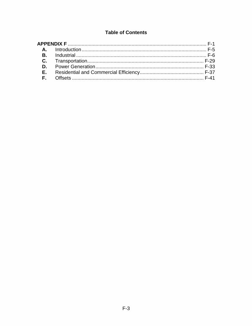
Table of Contents APPENDIX F .................................................................................................... F-1
A. Introduction.......................................................................................... F-5 B. Industrial .............................................................................................. F-6 C. Transportation.................................................................................... F-29 D. Power Generation.............................................................................. F-33 E. Residential and Commercial Efficiency.............................................. F-37 F. Offsets ............................................................................................... F-41

F-4
This Page Intentionally Left Blank
F-5
Appendix F Compliance Pathways Analysis
This Appendix outlines the assumptions and calculations used and the results generated in the compliance pathways analysis, the results of which are described in Staff Report Part I, Volume I, Chapter V: Compliance Pathways Scenarios.
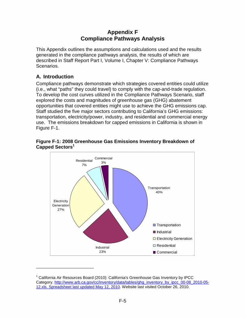
A. Introduction Compliance pathways demonstrate which strategies covered entities could utilize (i.e., what “paths” they could travel) to comply with the cap-and-trade regulation. To develop the cost curves utilized in the Compliance Pathways Scenario, staff explored the costs and magnitudes of greenhouse gas (GHG) abatement opportunities that covered entities might use to achieve the GHG emissions cap. Staff studied the five major sectors contributing to California’s GHG emissions: transportation, electricity/power, industry, and residential and commercial energy use. The emissions breakdown for capped emissions in California is shown in Figure F-1. Figure F-1: 2008 Greenhouse Gas Emissions Inventory Breakdown of Capped Sectors1
Transportation40%
Industrial23%
Residential7%
Electricity Generation
27%
Commercial3%
Transportation
Industrial
Electricity Generation
Residential
Commercial
1 California Air Resources Board (2010): California's Greenhouse Gas Inventory by IPCC Category. http://www.arb.ca.gov/cc/inventory/data/tables/ghg_inventory_by_ipcc_00-08_2010-05-12.xls. Spreadsheet last updated May 12, 2010. Website last visited October 26, 2010.
F-6
The sector with the largest contribution (40 percent) to California’s capped GHG emissions is the transportation sector, which includes personal vehicles, air traffic, ships at port, and trucks. The next largest contributor to capped GHG emissions is electricity, at 27 percent of emissions. This sector accounts for both in-state generation and electricity generated out of the State but imported into California. At 23 percent of total emissions, the industrial sector is the third largest producer of capped GHG emissions. Most emissions are associated with industries burning natural gas to produce steam and process heat; however, some industries burn coal, petroleum coke, refinery gas, biomass, and other fuels. The GHG emissions from fuels burned by the residential and commercial sector account for 10 percent of emissions in California. Most of these fuels are used to power heating, ventilation, and air conditioning systems.
The next several sections individually break down each sector and describe the emissions sources and abatement opportunities.
B. Industrial Most of the capped GHG emissions from the industrial sector are produced from burning fuel to create either steam or process heat. To analyze the GHG reductions in the industrial sector, strategies for steam and process heater systems were investigated across all industries. The exception to this methodology was the cement sector because high-temperature kilns operate differently from steam and process heater systems.
This section is divided by industrial sub-sectors: petroleum, oil and gas, chemicals, food, wood products, iron and steel, and cement. The methodology used to calculate the GHG reductions and costs of all industrial sectors used in the abatement curves is described below. Two accompanying spreadsheets include the results of this methodology along with the formulas (embedded in the spreadsheets) used in the calculations.2 Each of the sections from APPENDIX FB.2 to APPENDIX FB.15 corresponds to a tab in this spreadsheet.
Steam and process heating systems were chosen for compliance analysis because they are part of almost every major industrial process today. A large percentage of the fossil fuel burned in U.S. industry is burned to produce steam and process heat. Since industrial systems are diverse, but often have major steam and process heat systems in common, the analysis of improvement to steam and process heating systems is useful when projecting abatement over a number of industries using one analysis. Reductions in emissions from steam and process heating systems were only applied to all industries with greater than 20 percent of fuel used for steam or process heat (i.e., the petroleum, oil and gas, chemicals, food, and wood products sub-sectors). This was done to avoid unnecessary analysis where reductions are expected to be small.
2 See the “Supplemental Materials” section of the Cap-and-Trade Regulation website (http://www.arb.ca.gov/regact/2010/capandtrade10/capandtrade10.htm).
F-7
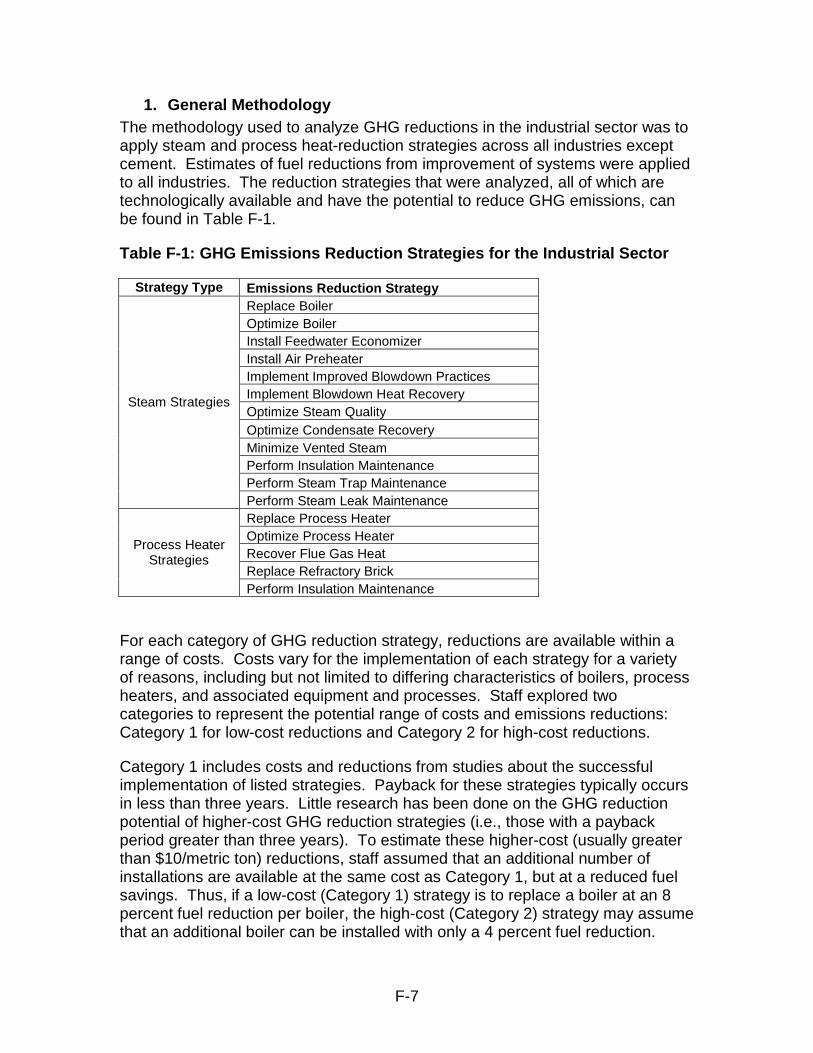
1. General Methodology The methodology used to analyze GHG reductions in the industrial sector was to apply steam and process heat-reduction strategies across all industries except cement. Estimates of fuel reductions from improvement of systems were applied to all industries. The reduction strategies that were analyzed, all of which are technologically available and have the potential to reduce GHG emissions, can be found in Table F-1.
Table F-1: GHG Emissions Reduction Strategies for the Industrial Sector
Strategy Type Emissions Reduction Strategy Replace Boiler Optimize Boiler Install Feedwater Economizer Install Air Preheater Implement Improved Blowdown Practices Implement Blowdown Heat Recovery Optimize Steam Quality Optimize Condensate Recovery Minimize Vented Steam Perform Insulation Maintenance Perform Steam Trap Maintenance
Steam Strategies
Perform Steam Leak Maintenance Replace Process Heater Optimize Process Heater Recover Flue Gas Heat Replace Refractory Brick
Process Heater Strategies
Perform Insulation Maintenance
For each category of GHG reduction strategy, reductions are available within a range of costs. Costs vary for the implementation of each strategy for a variety of reasons, including but not limited to differing characteristics of boilers, process heaters, and associated equipment and processes. Staff explored two categories to represent the potential range of costs and emissions reductions: Category 1 for low-cost reductions and Category 2 for high-cost reductions.
Category 1 includes costs and reductions from studies about the successful implementation of listed strategies. Payback for these strategies typically occurs in less than three years. Little research has been done on the GHG reduction potential of higher-cost GHG reduction strategies (i.e., those with a payback period greater than three years). To estimate these higher-cost (usually greater than $10/metric ton) reductions, staff assumed that an additional number of installations are available at the same cost as Category 1, but at a reduced fuel savings. Thus, if a low-cost (Category 1) strategy is to replace a boiler at an 8 percent fuel reduction per boiler, the high-cost (Category 2) strategy may assume that an additional boiler can be installed with only a 4 percent fuel reduction.
F-8
Because the fuel savings of the Category 2 boiler is cut in half, but the capital cost is the same, the Category 2 boiler will have a higher dollars-per-metric ton cost.
For each category, the number of installations of that strategy in California industries must be estimated. The estimates used in this study are the best available given the limited information about which technologies are capable of being applied to each of the covered entities. Without data from each firm on equipment used, the assumptions are only estimates. For steam reductions, a DOE report3 provides a number of estimates for the United States on the feasibility of each strategy. Due to the lack of California-specific data, staff applied the same U.S. feasibility estimates to California steam and process heat sectors. For process heat, less information was available, and steam system feasibilities were used where appropriate. For example, it was assumed that the percentage of process heaters that can be replaced is the same as the percentage of boilers than can be replaced.
All data, estimates, and calculations used for this analysis can be found embedded within the spreadsheets entitled “compathboiler.xls” and “compathprocessheat.xls,” both of which are available for download on the Cap-and-Trade Regulation website.4
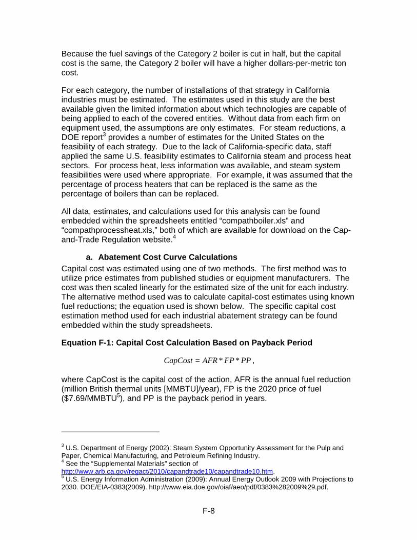
a. Abatement Cost Curve Calculations Capital cost was estimated using one of two methods. The first method was to utilize price estimates from published studies or equipment manufacturers. The cost was then scaled linearly for the estimated size of the unit for each industry. The alternative method used was to calculate capital-cost estimates using known fuel reductions; the equation used is shown below. The specific capital cost estimation method used for each industrial abatement strategy can be found embedded within the study spreadsheets.
Equation F-1: Capital Cost Calculation Based on Payback Period
PPFPAFRCapCost **= ,
where CapCost is the capital cost of the action, AFR is the annual fuel reduction (million British thermal units [MMBTU]/year), FP is the 2020 price of fuel ($7.69/MMBTU5), and PP is the payback period in years.
3 U.S. Department of Energy (2002): Steam System Opportunity Assessment for the Pulp and Paper, Chemical Manufacturing, and Petroleum Refining Industry. 4 See the “Supplemental Materials” section of http://www.arb.ca.gov/regact/2010/capandtrade10/capandtrade10.htm. 5 U.S. Energy Information Administration (2009): Annual Energy Outlook 2009 with Projections to 2030. DOE/EIA-0383(2009). http://www.eia.doe.gov/oiaf/aeo/pdf/0383%282009%29.pdf.
F-9
The number of units able to implement each strategy was calculated using feasibility percentages of each strategy and the total number of units available. Thus, if it is feasible to implement a strategy on 10 percent of boilers, and the total number of boilers is 90, nine installations of that strategy could be implemented during the period 2012–2020.
Equation F-2: Number of Units Implementing the Strategy
TotalNFn *= ,
where n is the total number of units on which the strategy could be implemented during the period 2012–2020, F is the feasibility percentage, and TotalN is the total number of units of a specific type (i.e., boilers, process heaters).
For maintenance activities, the reductions are calculated from the annual fuel reduction percentage and feasibility of applying the steam or process heat strategies.
Equation F-3: Total Annual Fuel Reduction from Maintenance Activity
FuelUseAFRPFTAFR **= ,
where TAFR is the total annual fuel reduction (MMBTU) of implementing that maintenance strategy for that industry, F is the feasibility percentage, AFRP is the annual fuel reduction percentage, and FuelUse is the fuel use of the unit (MMBTU) to which the maintenance activity is applied. AFRP per unit was determined from published studies and was usually provided as a percent reduction in fuel use of that unit.
The total GHG reduction from implementing all the strategies was calculated using the following equation:
Equation F-4: Total Greenhouse Gas Reduction
FIAFRnGHGR **= ,
where GHGR is the greenhouse gas reduction, n is the total number of units, AFR is the annual fuel reduction (MMBTU), and FI is the fuel intensity (million metric tons of CO2 equivalent (MMTCO2e)/ MMBTU) of the particular fuel. Scoping Plan carbon intensities of fuels were used. The following assumptions are used for fuel intensity:
• For natural gas combustion the emissions factors6 are
6 California Air Resources Board (2008): Climate Change Scoping Plan: A Framework for Change. http://www.arb.ca.gov/cc/scopingplan/document/adopted_scoping_plan.pdf.
F-10
o 5.3156 X 10⁻⁸ MMTCO2e/ MMBTU for commercial and residential combustion, and
o 5.3072 X 10⁻⁸ MMTCO2e/MMBTU for industrial and power generation use; and
• For sub-bituminous coal, the emissions factor7 is 9.2841 *10-8 MMTCO2e/MMBTU.
To calculate the cost per metric ton, the capital cost was annualized with the following equation:
Equation F-5: Annualized Capital Cost
( )
+−
×=
tr
rCapCostAnnCapCost
1
11
,
where AnnCapCost is the annualized capital cost, CapCost is the capital cost ($), r is the discount rate, and t is the life of the capital in years. Once annualized, the cost per metric ton is calculated using the calculation below.
Equation F-6: Cost of Strategy
GHGR
FPAFRAnnCapCostCPT
*−= ,
where CPT is cost per metric ton, AFR is the annual fuel reduction (MMBTU), FP is the 2020 price of fuel ($7.69/MMBTU5), and GHGR is the greenhouse gas reduction (MMTCO2e).
2. Develop Average Boiler and Process Heater8 To develop abatement strategies that apply to boiler and process heaters, the baseline boiler and process heater units must first be defined for each industrial sub-sector. The assumptions needed for boilers and process heaters were unit size (maximum rated fuel consumption per hour, MMBTU/hr), efficiency (percent of useful heat energy from fuel energy), and capacity (the ratio of actual load to the maximum load).
7 U.S. Energy Information Administration (1994): Quarterly Coal Report, January-April 1994. Washington, D.C.: DOE/EIA-0121(94/Q1).
8 See the “Average Boiler Size” sheet of compathboiler.xls for calculations.
F-11
Studies give a wide range of sizes for boilers in the food industry. One study references a very large dairy which runs a 125 MMBTU/hr boiler and has two other boilers at 70 MMBTU/hr, which do not run.9 On the other hand, a small poultry plant uses a 16.5 MMBTU/hr boiler with a backup 6.6 MMBTU/hr boiler.10 Another case study refers to a 40 MMBTU/hr boiler.11 Thus, a range of 10 to 100 MMBTU/hr boiler size was estimated for the food industry. Staff assumed an average size of 40 MMBTU/hr for food industry boilers. For process heaters in the food industry, only one study gave process heater sizes between 10 and 30 MMBTU/hr.9 Thus, staff assumed an average size of 20 MMBTU/hr for food industry process heaters.
The oil and gas industry also has a wide range of boiler sizes that vary depending on well size. A range of 50–100 MMBTU/hr boiler size was estimated for the oil and gas industry. Two San Joaquin Unified Air Pollution Control District best performance standards estimate the typical boiler size at 65 MMBTU/hr,12,13 which staff used as its average unit size estimate.
Boilers in the petroleum industry are expected to be large, given the size of petroleum facilities. Staff assumed boilers to be over 60 MMBTU/hr in the petroleum industry and assumed an average boiler size of 100 MMBTU/hr. Process heaters are also in this size range, so staff assumed an average process heater size of 100 MMBTU/hr.
The wood and chemical industry use large amounts of steam, and were therefore expected to have boilers larger than the food industry but smaller than the petroleum industry. Thus, staff assumed sizes to be greater than 50 MMBTU/hr and an average boiler size of 60 MMBTU/hr. For process heaters, staff assumed a size of 50 MMBTU/hr. This size was chosen to be larger than process heaters in the food industry but smaller than those used in the petroleum industry.
In the iron and steel industry, process heaters are expected to be fairly large given the high percentage of fuel used by the industry to produce heat. However, facilities are smaller than chemical industries; thus, staff assumed an average size of 40 MMBTU/hr. This size is larger than the food industry, which uses a smaller portion of process heat, but slightly smaller than the chemical industry, which has larger facilities.
Boiler efficiency in the food industry was estimated to range between 82 and 83 percent.14,15 In the oil and gas industry, boiler efficiency was estimated to range
9 U.S. Department of Energy (2005): ESA Conducted at Dairyman's Land O' Lakes Plant. 10 U.S. Department of Energy (2008): Final Public Report for ESA-188-3. 11 Calculated from U.S. Department of Energy (2008): Final Public Report for ESA-167-3. 12 Roberts and Keast (2010): Best Performance Standard Boilers. San Joaquin Valley Unified Air Pollution Control District. 13 Roeder and Marjollet (2010): Best Performance Standard Oilfield Steam Generator. San Joaquin Valley Unified Air Pollution Control District. 14 U.S. Department of Energy (2006): ESA-178 Final Public Report.
F-12
between 77 and 82 percent.12,13 Without any case studies to estimate boiler efficiency for the petroleum, wood product, or chemical industries, staff assumed a range of 80 to 83 percent. Because no information on process heater efficiencies was available, staff utilized the full range of boiler efficiencies to process heaters (77 to 83 percent). Staff used a wider range of process heater efficiencies because of the uncertainty given the lack of information on the units.
Several case studies on the food industry can be used to calculate a boiler capacity of approximately 80 percent. 9,14,15 This capacity was applied to the wood products industry, which, like the food industry, was noted in some studies to shut down nights and/or weekends. The chemical and oil and gas industries were assumed to have a higher capacity, as boilers usually run continuously all year. Petroleum boilers are expected to have the highest capacity, given the large size and integrated nature of the industry. Similar capacities were used for process heaters.
With the assumptions developed, staff calculated fuel use per unit for each of the industries.
3. Boiler/Process Heater Replacement16 Boilers and process heaters are infrequently replaced for the purpose of fuel savings; instead, units are typically replaced once they have surpassed their useful life and maintenance becomes too expensive. However, it is possible that this proposed regulation could incentivize early retirement of boilers and process heaters and replacement with new, high-efficiency units. To account for this greenhouse gas abatement opportunity, boiler replacement is estimated in addition to normal retirement.
Staff assumed that each replacement boiler and process heater has an efficiency of 88 percent, which San Joaquin Unified Air Pollution Control District has set as a goal for new boilers.13 Staff applied the same 88 percent efficiency to process heaters in the absence of any other estimates.
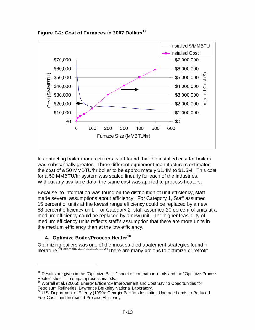
Boiler costs were obtained from direct communication with manufacturers and a U.S. Department of Energy (DOE) publication on Process Equipment Cost Estimates.17 Using estimates from the DOE paper, the cost of furnaces is given in Figure F-2. From Figure F-2, the cost per size ($/MMBTU/hr) is fairly constant for boiler sizes 50–200 MMBTU/hr; thus, it was assumed that the cost of boilers and process heaters can be scaled linearly with size.
15 U.S. Department of Energy (2008): Final Public Report for ESA-167-3. 16 Results given in the “Replace Boiler” sheet of compathboiler.xls and the “Replace Process Heater” sheet of compathprocessheat.xls. 17 Loh et al. (2002): Process Equipment Cost Estimation. U.S. Department of Energy.
F-13
Figure F-2: Cost of Furnaces in 2007 Dollars17
$0
$10,000
$20,000
$30,000
$40,000
$50,000
$60,000
$70,000
0 100 200 300 400 500 600
Furnace Size (MMBTU/hr)
Cos
t ($/
MM
BT
U)
$0
$1,000,000
$2,000,000
$3,000,000
$4,000,000
$5,000,000
$6,000,000
$7,000,000
Inst
alle
d C
ost (
$)
Installed $/MMBTU
Installed Cost
In contacting boiler manufacturers, staff found that the installed cost for boilers was substantially greater. Three different equipment manufacturers estimated the cost of a 50 MMBTU/hr boiler to be approximately $1.4M to $1.5M. This cost for a 50 MMBTU/hr system was scaled linearly for each of the industries. Without any available data, the same cost was applied to process heaters.
Because no information was found on the distribution of unit efficiency, staff made several assumptions about efficiency. For Category 1, Staff assumed 15 percent of units at the lowest range efficiency could be replaced by a new 88 percent efficiency unit. For Category 2, staff assumed 20 percent of units at a medium efficiency could be replaced by a new unit. The higher feasibility of medium efficiency units reflects staff’s assumption that there are more units in the medium efficiency than at the low efficiency.
4. Optimize Boiler/Process Heater18 Optimizing boilers was one of the most studied abatement strategies found in literature.for example, 3,19,20,21,22,23,24There are many options to optimize or retrofit
18 Results are given in the “Optimize Boiler” sheet of compathboiler.xls and the “Optimize Process Heater” sheet” of compathprocessheat.xls. 19 Worrell et al. (2005): Energy Efficiency Improvement and Cost Saving Opportunities for Petroleum Refineries. Lawrence Berkeley National Laboratory. 20 U.S. Department of Energy (1999): Georgia-Pacific's Insulation Upgrade Leads to Reduced Fuel Costs and Increased Process Efficiency.
F-14
existing boilers to increase efficiency, including reducing the amount of air used in combustion. The more air used to burn the fuel, the more heat is wasted in heating air. Air slightly in excess of the ideal stochiometric fuel-to-air ratio is required for safety and to reduce nitrogen oxide (NOx) emissions, but approximately 15 percent excess air is adequate.22 However, many boilers operate using greater amounts of excess air than is necessary. Thus, there is a range of excess air that can be reduced to increase boiler efficiency. The range of reduction potential of reducing excess air is 0.5 to 5 percent fuel savings. Staff assumed an average 2 percent fuel reduction for boiler efficiency for Category 1. For Category 2, staff assumed less excess air was available, and only a 1 percent efficiency gain was available.
A DOE study estimates that the efficiency increases of process heaters from better control of the air-to-fuel ratio is estimated to be 5 to 25 percent.25 However, the abatement strategy for process heating is nearly identical to that for boiler heaters. In comparing the two strategies, staff found the DOE estimate for process heaters to be too high, and therefore assumed the same efficiency increases (2 percent for Category 1 and 1 percent for Category 2) for process heaters as for boilers.
Two separate studies give the payback period for boiler efficiency as six months.3,26 Staff chose to err on the side of higher prices, and assumed a one year payback for Category 1 with a 2 percent fuel reduction per unit for both boilers and process heaters. For Category 2, staff assumed a 50 percent price increase from Category 1 for both boilers and process heaters. This price increase was included to account for additional controls and/or flue gas monitoring that would be necessary to achieve the additional 1 percent fuel reduction in Category 2.
From a DOE report, the feasibility of implementing boiler efficiency in the wood products, chemical, and petroleum refining industries is given as 34 percent.3 Thus, for Category 1, staff assumed that 34 percent of boilers could implement boiler efficiency strategies and achieve a 2 percent reduction in fuel consumption.
21 Martin et al. (2000): Opportunities to Improve Energy Efficiency and Reduce Greenhouse Gas Emissions in the U.S. Pulp and Paper Industry. Lawrence Berkeley National Laboratory. 22 Einstein et al. (2001): Steam Systems in Industry: Energy Use and Energy Efficiency Improvement Potentials. Lawrence Berkeley National Laboratory. 23 U.S. Department of Energy (2002): Martinez Refinery Completes Plant-Wide Energy Assessment. 24 U.S. Department of Energy (2003): Paramount Petroleum: Plant-Wide Energy Efficiency Assessment Identifies Three Projects. 25 U.S. Department of Energy (2008): Improving Process Heating System Performance: A Sourcebook for Industry. 26 U.S. Department of Energy (2002): Appleton Paper Plant-Wide Energy Assessment Saves Energy and Reduces Waste.
F-15
For Category 2, a 20 percent increase in feasibility from Category 1 was assumed. This assumption is based on staff’s belief that there are a greater number of boilers that can be further optimized with additional controls and/or flue gas monitoring.
5. Boiler Feedwater Economizer and Process Heater Flue Gas Heat Recovery27
Boiler feedwater economizer and process heater flue gas heat recovery both take energy from the flue gas to preheat the working fluid (water for boilers and air for process heaters). These strategies entail installing additional stack piping that is convection heated by the flue gas. The preheated fluid is then piped to the inlet of the boiler/process heater at an elevated temperature.
Several studies identify the range of fuel reduction percentages in implementing a boiler feedwater economizer as between 1 and 6 percent.for example, 15,25,28,29, 30 Because refinery stack temperatures are usually low, staff estimated the reduction potential in petroleum refineries at 2 percent. Because the chemical industry is largely associated with hydrogen production for petroleum refining, staff also assumes a 2 percent reduction for the chemical industry. Staff estimated a 3.5 percent efficiency increase from implementation of a mixture of conventional and condensing economizers for all other industries, and assumed the fuel reduction for Category 2 to be half of that for Category 1.
A 2008 DOE25 report on process heater flue gas recovery listed the fuel reduction at between 15 and 30 percent. Because this reduction strategy is similar to retrofitting a boiler with a feedwater economizer, and because published fuel reduction estimates for feedwater economizers are much lower, staff found these DOE reductions to be much too high. Staff chose to use the same fuel reduction assumptions for process heater flue gas recovery as it used for boiler feedwater economizers, given the similarities.
The simple payback period for a boiler feedwater economizer is approximately two to five years using a fuel reduction of 3 percent.3,31 Staff contacted manufacturers about the cost to retrofit a boiler with a feedwater economizer, and their quotes were between $150,000 and $500,000 for a 50 MMBTU/hr unit. Thus, for this analysis, staff estimated that a boiler retrofit with a feedwater economizer is approximately $250,000 for a 50 MMBTU/hr, which equates to a
27 Results given in the “Feedwater Economizer” sheet of compathboiler.xls and the “Recover Flue Gas Heat” sheet of compathprocessheat.xls. 28 U.S. Department of Energy (2006): ESA-014. 29 U.S. Department of Energy (2006): SCA Tissue North America Public Report (ESA-042). 30 The Natural Gas Consortium: Solutions for Efficiency, Emissions, and Cost Controls (2007): Boiler Burner Economizers. http://www.energysolutionscenter.org/boilerburner/Eff_Improve/Efficiency/Economizers.asp. 31 Chimack et al. (2003): Energy Conservation Opportunities in the Pulp and Paper Industry: An Illinois Case Study. Energy Resources Center, University of Illinois at Chicago.
F-16
2.6 year simple payback when using a 3.5 percent fuel reduction, and a 4.1 year simple payback when using a 2 percent fuel reduction. Staff assumed that the cost of boiler retrofits scale linearly with size in the range of boilers analyzed (40–100 MMBTU/hr). Category 2 used the same capital cost as Category 1.
Because staff found no cost estimates for process heater flue gas heat recovery, it assumed a simple payback period of 3.5 years for all industries to match the average cost per ton of Category 1 boiler feedwater economizers. Category 2 used the same capital cost as Category 1.
A DOE study estimates that the percent of facilities where a boiler feedwater economizer could be implemented is between 10 and 14 percent.3 Staff estimated that the feasibility is slightly larger (at 15 percent) than that estimated in the DOE study because technologies developed over the lifetime of the cap-and-trade program may make this measure feasible on more boilers. No data were found on the feasibility of process heater flue gas heat recovery; thus, staff applied a 15 percent feasibility to all industries. For Category 2, staff estimated a 20 percent increase in feasibility from Category 1 because it believes that additional heat can be extracted from flue gas from boiler and process heater units, albeit at high costs.
6. Process Heater Refractory Brick Maintenance32 Refractory bricks are high-temperature materials used to make furnaces’ inner liners, which are used in process heaters. Even though the material retains its strength under high thermal load, it will slowly degrade over time. As refractory bricks degrade, heat is lost to surroundings, which decreases the efficiency of the furnace. Regular maintenance and replacement is needed to retain efficiency.
Fuel reductions from refractory brick maintenance ranges from 1 to 20 percent.3,25 Staff used the DOE estimate of 1 percent fuel reduction for Category 1, and half the fuel reduction (0.5 percent) for Category 2.
Using the DOE report, the payback period for refractory brick maintenance is approximately 1.2 years, which staff used to calculate the cost for Category 1. Staff used the same capital cost for Category 2 as was calculated in Category 1.
The DOE report also estimates that 4 percent of facilities can implement refractory brick maintenance and achieve the estimated reductions. Staff used this feasibility percentage for Category 1. Category 2 was estimated to have a 20 percent greater feasibility than Category 1 because staff assumed that a greater number of high cost strategies exist because those strategies are currently not cost effective, and thus have not been implemented.
32 Results given in the “Replace Refractory Brick” sheet of compathprocessheat.xls.
F-17
7. Boiler Air Preheater33 Combustion air preheaters improve boiler efficiency by transferring available energy from the exhaust flue gas to the incoming combustion air. This is similar to a boiler feedwater economizer in that additional piping is installed in the convection section of the stack. The difference is that boiler air preheaters do not preheat the working fluid (steam), but instead preheat air prior to combustion. By having a higher inlet air temperature to the combustion chamber, less fuel is needed to heat the air to the desired temperature.
Assumptions were used directly from a DOE paper.3 For Category 1, staff used the same fuel savings estimates as that in the paper: 1.5 to 1.9 percent, depending on the industry. For Category 2, staff assumed the available fuel savings were half of Category 1. Staff also used the payback period estimated in this study: two to three years, depending on industry. For Category 2, staff assumed the same capital cost as Category 1. For this abatement strategy, the DOE study estimated what staff perceives to be a low feasibility: 3.0 to 3.5 percent. Staff chose to use a feasibility estimate higher than DOE’s estimate (5 percent feasibility for all industries) to reflect the belief that technologies developed before 2020 may make this measure available on more boilers. For Category 2, staff assumed a 20 percent increase in feasibility from Category 1 because those Category 2 strategies are currently not cost effective.
8. Improve Boiler Blowdown Practices34 Even with the best pretreatment programs, boiler feedwater often contains some degree of impurities, such as suspended and dissolved solids. The impurities can remain and accumulate inside the boiler as the boiler operation continues. The increasing concentration of dissolved solids may lead to carryover of boiler water into the steam, causing damage to piping, steam traps, and even process equipment. The increasing concentration of suspended solids can form sludge, which impairs boiler efficiency and heat transfer capability.35
To avoid boiler problems, water must be periodically discharged or “blown down” from the boiler to control the concentrations of suspended and total dissolved solids in the boiler. Surface water blowdown is often done continuously to reduce the level of dissolved solids, and bottom blowdown is performed periodically to remove sludge from the bottom of the boiler.35
The importance of boiler blowdown is often overlooked. Improper blowdown can cause increased fuel consumption, additional chemical treatment requirements, and heat loss. In addition, the blowdown water has the same temperature and
33 Results given in the “Air Preheater” sheet of compathboiler.xls. 34 Results given in the “Blowdown Practices” sheet of compathboiler.xls. 35 North Carolina Division of Pollution Prevention and Environmental Assistance (2004): Boiler Blowdown. http://www.p2pays.org/ref/34/33027.pdf.
F-18
pressure as the boiler water. This blowdown heat can be recovered and reused in the boiler operations.35
Several studies identify improving boiler blowdown practices by decreasing blowdown as an abatement strategy.3,10,14,28,36 Studies show that decreasing boiler blowdown can achieve 1 to 2 percent fuel reductions. Two categories were identified for this strategy. Category 1 analyzed blowdown reduction due to additional controls, such as automatic blowdown controllers. For Category 1, staff assumed the low end of the potential fuel savings from this strategy, 1 percent. Category 2 analyzed blowdown reduction due to increased boiler feedwater cleanup. By decreasing the contaminants in water, less boiler blowdown is needed to clean them out. For Category 2, staff assumed the high end of the potential fuel savings from this strategy, 2 percent.
From the studies, the estimated payback period of implementing automatic blowdown controls is estimated to be one to three years based on a 2 to 5 percent fuel reduction. Because Category 1 is only considered a 1 percent fuel reduction, staff assumed the high side of the payback period, three years.
For Category 2, it is estimated that the cost of feedwater cleanup is much greater than automatic controls identified in Category 1. With no studies on which to base costs, staff assumed a simple payback of four years, to be greater than Category 1.
The feasibility of Category 1 (decreased blowdown with additional controls) is limited because most industries consider this common practice. This is reflected in the low feasibility of 8.5 to 12.3 percent.3 The feasibility of Category 2 assumed to be much larger than Category 1. This is to reflect the robustness of implementing feedwater cleanup to reduce blowdown. Even systems that implement Category 1 can further reduce boiler blowdown with cleaner inlet water. Thus, staff assumed an increase of Category 1 feasibility by 50 percent.
9. Boiler Blowdown Heat Recovery37 Blowdown water has the same temperature and pressure as the boiler water, and its heat can be recovered and reused in the boiler operations. Blowdown heat recovery uses a heat exchanger to transfer heat from the blowdown to the boiler feedwater. Several studies identify heat recovery from blowdown steam as an abatement opportunity.19,38,39,40 The fuel reduction calculated from these
36 U.S. Department of Energy (2001): Installation of Reverse Osmosis Unit Reduces Refinery Energy Consumption. 37 Results given in the “Blowdown Heat Recovery” sheet of compathboiler.xls. 38 Lawrence Berkeley National Laboratory (2008): Energy Efficiency and Cost Saving Opportunities for the Glass Industry. 39 U.S. Department of Energy (2002): Boiler Blowdown Heat Recovery Project Reduces Steam System Energy Losses at Augusta Newsprint. 40 U.S. Department of Energy (2004): Improving Steam System Performance - A Sourcebook for Industry.
F-19
studies is given between 0.7 and 1.5 percent. Staff assumed that Category 1 implementation of boiler heat recovery had a fuel reduction of 1 percent. For Category 2, the fuel reduction was reduced to half (0.5 percent), at the same cost.
The simple payback of implementing boiler blowdown heat recovery was given in studies to be between 0.7 and 2.7 years for a 0.7 to 1.3 percent fuel reduction. Staff assumed a two-year payback period for Category 1, with a 1 percent fuel reduction. For Category 2, staff assumed the same cost as Category 1.
A DOE study sites the feasibility of this reduction at between 11 and 14 percent, depending on the industry.3 Staff assumed the high side of this estimate and used 15 percent feasibility for all industries. Staff’s assumption that the feasibility is slightly larger than the range given reflects that the cap-and-trade program lasts until 2020 and future technologies may make this measure available on more boilers. For Category 2, staff assumed a 20 percent increase in feasibility from Category 1. There exist a greater number of high-cost abatement strategies that have not been adopted because they are not cost effective.
10. Optimize Steam Quality41 Steam quality is a measure of the moisture content in the steam. Poor steam quality has an adverse effect on system equipment, particularly on valves, turbines, and heat exchangers. The primary cause of poor steam quality is boiler water carryover, which can be the result of a water treatment problem, high boiler-water level, and/or sudden drop in boiler or system pressure. A decrease in steam quality reduces the available energy in a delivered quantity of steam. Similarly, improving steam quality can reduce the amount of steam necessary to meet a particular set of end-use requirements.3 To optimize the steam quality, additional controls and metering may need to be installed to ensure that the steam is to specification.
Fuel reduction attributed to this strategy was approximately 1 percent.3,15 Staff used this fuel reduction for Category 1. For Category 2, the fuel reduction was decreased to half of the value used for Category 1.
The simple payback for optimizing steam quality is estimated to be 0.8 to 1.5 years.3,15 For this analysis, the simple payback was assumed to be 1.5 years for Category 1. For Category 2, the same capital costs were used.
Staff used a DOE study3 to give a feasibility of implementing this strategy for each of the industries: 5.8 to 11.3 percent. For Category 2 the feasibility was assumed to be 7 to 13.5 percent—20 percent larger than Category 1. There exist a greater number of high-cost abatement strategies that have not been adopted because they are not cost effective.
41 Results given in the “Optimize Steam Quality” sheet of compathboiler.xls.
F-20
11. Optimize Condensate Recovery42 As steam is cooled during transport around the facility, steam traps capture liquid condensate. In many cases, this condensate is piped into the wastewater stream even though the condensate is still at elevated temperature, and therefore still useful in transferring heat to feedwater or being directly piped into the feedwater. Several studies identify this as a potential abatement opportunity. 10,15,19,28
Case studies show that optimizing condensate recovery could result in a possible 0.3 to 0.4 percent reduction in boiler fuel use. Staff estimated a fuel reduction of 0.4 percent for Category 1, and a fuel reduction of 0.2 percent for Category 2.
Staff found no data on the feasibility of implementing this strategy. Because this strategy yields small fuel reductions, staff assumes that the strategy is mostly overlooked, and assumed a feasibility of 20 percent for Category 1. For Category 2, where reductions are even less, staff estimated a feasibility of 24 percent (i.e., 20 percent greater than Category 1). There exist a greater number of high-cost abatement strategies that have not been adopted because they are not cost effective.
12. Minimize Vented Steam43 This abatement strategy refers to improvements that reduce the amount of steam release caused by oversupply. Steam oversupply generally results from poor boiler steam output control, insufficient boiler turndown, erratic steam demand, excessive numbers (capacity) of back-pressure turbines operating, and failed steam traps discharging live steam into lower-pressure steam systems. Common methods used to eliminate vent steam include replacing steam turbines with electric motor drives, improving boiler controls, installing steam accumulators, and replacing failed traps.3
Staff assumed a fuel reduction percentage consistent with a DOE study that explored this abatement strategy.3 The fuel reduction percentage given was between 2.3 and 3.0 percent, depending on the industry. Staff assumed those reductions for Category 1, and assumed half of those reductions for Category 2.
Staff also assumed a simple payback consistent with the DOE paper. The payback period given was very short, at less than one year. For Category 1, costs were calculated using a simple payback of six months. The same capital costs were used for Category 2, but with 50 percent less fuel reductions achieved.
For Category 1 feasibility, staff used the DOE estimates (4.1 to 6.4 percent, depending on industry). For Category 2, staff assumed a 20 percent increase in feasibility of Category 1. There exist a greater number of high-cost abatement strategies that have not been adopted because they are not cost effective.
42 Results given in the “Optimize Condensate Recovery” sheet of compathboiler.xls. 43 Results given in the “Minimize Vented Steam” sheet of compathboiler.xls.
F-21
13. Insulation Maintenance44 Because steam and process heat is transferred throughout facilities to perform or be used in processes, heat is lost to surroundings from pipes. To reduce this heat loss, most pipes and vessels are insulated. Insulation, however, ages and must undergo maintenance and replacement to ensure that the equipment is well insulated. Also, insulating materials continue to advance with lower heat capacities. Several studies identify insulation as a potential fuel reduction opportunity.20,23,31,45,46
Fuel reductions from insulation maintenance in the studies range from 0.5 to 7.5 percent. A DOE paper3 provides a breakdown of insulation condition in steam systems. When systems are adequately insulated, approximately 3.5 percent less fuel will be used; staff assumed this reduction strategy to be Category 1. To insulate systems that were not insulated, the fuel reduction is approximately 7.5 percent, which staff assumed was Category 2. This percent fuel reduction was carried over to the process heater assumptions for insulation maintenance.
The DOE paper also provides estimated payback periods for insulation. A payback of one to 1.5 years was estimated in this paper. Staff assumed a payback period of 2 years for Category 1 and 3 years for Category 2. The increased payback periods are to account for additional maintenance and upkeep to ensure adequate insulation. These paybacks were also used for process heater insulation maintenance.
To estimate feasibility, the DOE paper gives a breakdown of the percentage of industries with inadequate and uninsulated steam systems. From the study, it was estimated that 40 percent of facilities have inadequate insulation and 5 percent of facilities have uninsulated steam systems. Staff used these feasibilities for both steam and process heat systems.
14. Steam Trap Maintenance47 As steam cools, it begins to condense and is removed by a steam trap. Steam traps come in many different configurations, but all allow condensate to pass through while blocking the passage of steam. Steam traps slowly corrode and require regular maintenance or replacement. If they are not maintained, steam traps will allow steam and condensate to pass, wasting significant amounts of steam. Along with maintenance and replacement, automated steam trap monitoring is available at an increased price. Nearly every study on steam systems identified this as a potential strategy to reduce fuel use.
44 Results given in the “Insulation Maintenance” sheet of compathboiler.xls and the “Insulation Maintenance” sheet of compathprocessheat.xls. 45 U.S. Department of Energy (2006): 10 Tips for Saving Natural Gas in Steam Systems. 46 U.S. Department of Energy (2010): IAC Case Study Database. http://iac.rutgers.edu/database/. 47 Results given in the “Steam Trap Maintenance” sheet of compathboiler.xls.
F-22
Fuel reductions from steam trap maintenance in the studies range from 0.3 to 10 percent. A DOE paper3 provides a breakdown of steam trap maintenance conditions. Performing maintenance on steam systems with poorly maintained steam traps yields a reduction of 3 percent, which staff assumed for Category 1 analysis. Performing maintenance on facilities that do not maintain traps will result in a fuel reduction of 5 percent, which staff assumed for Category 2 analysis.
The payback period for steam trap maintenance ranges from a couple months to one year. Staff assumed a simple payback period for Category 1 to be one year. For Category 2, staff assumed a 50 percent increase in cost from Category 1. This cost increase reflects additional monitoring and maintenance.
To estimate feasibility, the DOE paper gives a breakdown of the percentage of industries with steam traps that were informally maintained or not maintained at all. The study estimated that 50 percent of facilities have steam traps that could benefit from improved maintenance and that 30 percent of facilities do not maintain steam traps. Staff applied the 50 percent to Category 1 feasibility and 30 percent to Category 2.
15. Steam Leak Maintenance48 Another area of steam leakage is directly from pipes and fittings. Over time, pipes and fittings can corrode and may begin to leak steam. To mitigate this, pipe and fitting maintenance is required, to repair any leaks that occur. As with steam trap maintenance, many studies investigated steam leak maintenance as a potential strategy to reduce fuel use.
In the studies, fuel reductions from steam trap maintenance range from 0.3 to 10 percent. A DOE paper3 provides a breakdown of steam leak maintenance conditions. Performing maintenance on steam systems with poorly maintained steam traps yields a fuel reduction of 3 percent, which staff assumed for Category 1 analyses. Performing maintenance on facilities that do not maintain traps will result in a fuel reduction of 5 percent, which staff assumed for Category 2 analyses.
The payback period for steam trap maintenance ranges from a couple months to one year. Staff assumed a simple payback period for Category 1 to be one year. For Category 2, staff assumed a 50 percent increase in cost from Category 1. This increase in cost reflects additional monitoring and maintenance.
To estimate feasibility, the DOE paper gives a breakdown of the percentage of industries with steam traps that were informally maintained and not maintained at all. The study estimated that 50 percent of facilities have steam traps that could benefit from improved maintenance, and that 30 percent of facilities do not
48 Results given in the “Steam Leak Maintenance” sheet of compathboiler.xls.
F-23
maintain steam traps. Staff applied the 50 percent to Category 1 feasibility and 30 percent to Category 2.
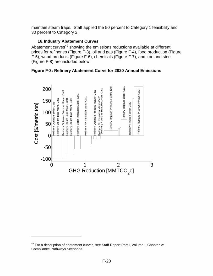
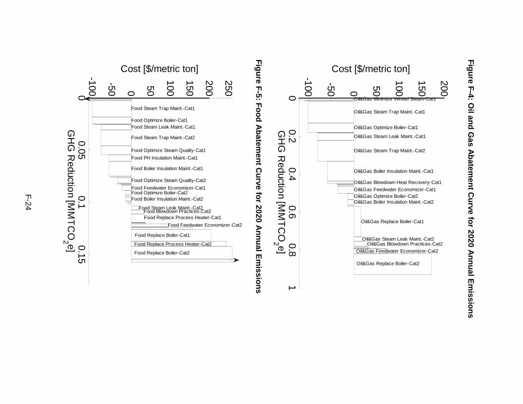
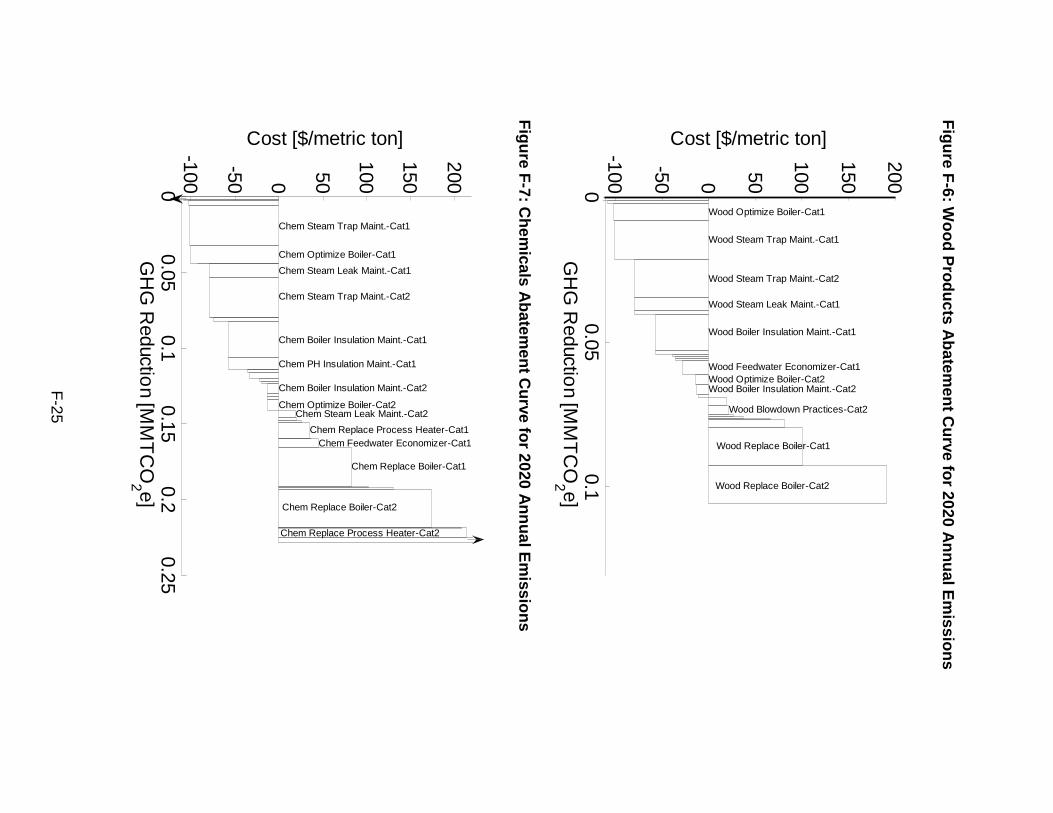
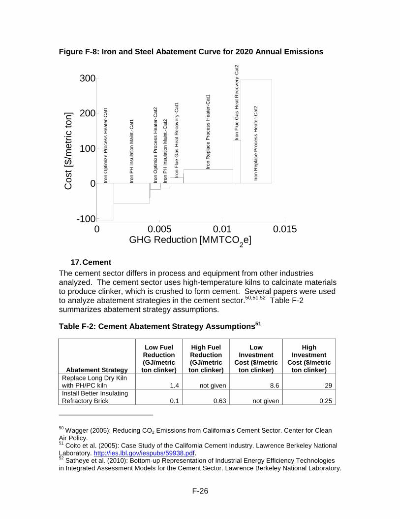
16. Industry Abatement Curves Abatement curves49 showing the emissions reductions available at different prices for refineries (Figure F-3), oil and gas (Figure F-4), food production (Figure F-5), wood products (Figure F-6), chemicals (Figure F-7), and iron and steel (Figure F-8) are included below.
Figure F-3: Refinery Abatement Curve for 2020 Annual Emissions
0 1 2 3-100
-50
0
50
100
150
200
Cos
t [$/
met
ric to
n]
GHG Reduction [MMTCO2e]
Ref
iner
y O
ptim
ize
Boi
ler-
Cat
1
Ref
iner
y S
team
Tra
p M
aint
.-C
at1
Ref
iner
y O
ptim
ize
Pro
cess
Hea
ter-
Cat
1
Ref
iner
y S
team
Lea
k M
aint
.-C
at1
Ref
iner
y S
team
Tra
p M
aint
.-C
at2
Ref
iner
y B
oile
r In
sula
tion
Mai
nt.-
Cat
1
Ref
iner
y P
H In
sula
tion
Mai
nt.-
Cat
1
Ref
iner
y O
ptim
ize
Pro
cess
Hea
ter-
Cat
2
Ref
iner
y P
H In
sula
tion
Mai
nt.-
Cat
2R
efin
ery
Flu
e G
as H
eat R
ecov
ery-
Cat
1
Ref
iner
y R
epla
ce P
roce
ss H
eate
r-C
at1
Ref
iner
y R
epla
ce B
oile
r-C
at1
Ref
iner
y R
epla
ce B
oile
r-C
at2
Ref
iner
y R
epla
ce P
roce
ss H
eate
r-C
at2
49 For a description of abatement curves, see Staff Report Part I, Volume I, Chapter V: Compliance Pathways Scenarios.
F
-24
Fig
ure F
-4: Oil an
d G
as Ab
atemen
t Cu
rve for 2020 A
nn
ual E
missio
ns
00.2
0.40.6
0.81
-100
-50 0 50
100
150
200Cost [$/metric ton]
GH
G R
eduction [M
MT
CO
2 e]
Oil&Gas Minimize Vented Steam-Cat1
Oil&Gas Steam Trap Maint.-Cat1
Oil&Gas Optimize Boiler-Cat1
Oil&Gas Steam Leak Maint.-Cat1
Oil&Gas Steam Trap Maint.-Cat2
Oil&Gas Boiler Insulation Maint.-Cat1
Oil&Gas Blowdown Heat Recovery-Cat1
Oil&Gas Feedwater Economizer-Cat1Oil&Gas Optimize Boiler-Cat2Oil&Gas Boiler Insulation Maint.-Cat2
Oil&Gas Replace Boiler-Cat1
Oil&Gas Steam Leak Maint.-Cat2Oil&Gas Blowdown Practices-Cat2
Oil&Gas Feedwater Economizer-Cat2
Oil&Gas Replace Boiler-Cat2
Fig
ure F
-5: Fo
od
Ab
atemen
t Cu
rve for 2020 A
nn
ual E
missio
ns
00.05
0.10.15
-100
-50 0 50
100
150
200
250
Cost [$/metric ton]
GH
G R
eduction [M
MT
CO
2 e]
Food Steam Trap Maint.-Cat1
Food Optimize Boiler-Cat1Food Steam Leak Maint.-Cat1
Food Steam Trap Maint.-Cat2
Food Optimize Steam Quality-Cat1
Food PH Insulation Maint.-Cat1
Food Boiler Insulation Maint.-Cat1
Food Optimize Steam Quality-Cat2
Food Feedwater Economizer-Cat1Food Optimize Boiler-Cat2Food Boiler Insulation Maint.-Cat2
Food Steam Leak Maint.-Cat2Food Blowdown Practices-Cat2Food Replace Process Heater-Cat1
Food Feedwater Economizer-Cat2
Food Replace Boiler-Cat1
Food Replace Process Heater-Cat2
Food Replace Boiler-Cat2
F
-25
Fig
ure F
-6: Wo
od
Pro
du
cts Ab
atemen
t Cu
rve for 2020 A
nn
ual E
missio
ns
00.05
0.1-100
-50 0 50
100
150
200Cost [$/metric ton]
GH
G R
eduction [M
MT
CO
2 e]
Wood Optimize Boiler-Cat1
Wood Steam Trap Maint.-Cat1
Wood Steam Trap Maint.-Cat2
Wood Steam Leak Maint.-Cat1
Wood Boiler Insulation Maint.-Cat1
Wood Feedwater Economizer-Cat1Wood Optimize Boiler-Cat2Wood Boiler Insulation Maint.-Cat2
Wood Blowdown Practices-Cat2
Wood Replace Boiler-Cat1
Wood Replace Boiler-Cat2
Fig
ure F
-7: Ch
emicals A
batem
ent C
urve fo
r 2020 An
nu
al Em
ission
s
00.05
0.10.15
0.20.25
-100
-50 0 50
100
150
200
Cost [$/metric ton]
GH
G R
eduction [M
MT
CO
2 e]
Chem Steam Trap Maint.-Cat1
Chem Optimize Boiler-Cat1
Chem Steam Leak Maint.-Cat1
Chem Steam Trap Maint.-Cat2
Chem Boiler Insulation Maint.-Cat1
Chem PH Insulation Maint.-Cat1
Chem Boiler Insulation Maint.-Cat2
Chem Optimize Boiler-Cat2Chem Steam Leak Maint.-Cat2
Chem Replace Process Heater-Cat1Chem Feedwater Economizer-Cat1
Chem Replace Boiler-Cat1
Chem Replace Boiler-Cat2
Chem Replace Process Heater-Cat2
F-26
Figure F-8: Iron and Steel Abatement Curve for 2020 Annual Emissions
0 0.005 0.01 0.015-100
0
100
200
300C
ost [
$/m
etric
ton]
GHG Reduction [MMTCO2e]
Iron
Opt
imiz
e P
roce
ss H
eate
r-C
at1
Iron
PH
Insu
latio
n M
aint
.-C
at1
Iron
Opt
imiz
e P
roce
ss H
eate
r-C
at2
Iron
PH
Insu
latio
n M
aint
.-C
at2
Iron
Flu
e G
as H
eat R
ecov
ery-
Cat
1
Iron
Rep
lace
Pro
cess
Hea
ter-
Cat
1
Iron
Flu
e G
as H
eat R
ecov
ery-
Cat
2
Iron
Rep
lace
Pro
cess
Hea
ter-
Cat
2
17. Cement The cement sector differs in process and equipment from other industries analyzed. The cement sector uses high-temperature kilns to calcinate materials to produce clinker, which is crushed to form cement. Several papers were used to analyze abatement strategies in the cement sector.50,51,52 Table F-2 summarizes abatement strategy assumptions.
Table F-2: Cement Abatement Strategy Assumptions51
Abatement Strategy
Low Fuel Reduction (GJ/metric ton clinker)
High Fuel Reduction (GJ/metric ton clinker)
Low Investment
Cost ($/metric ton clinker)
High Investment
Cost ($/metric ton clinker)
Replace Long Dry Kiln with PH/PC kiln 1.4 not given 8.6 29 Install Better Insulating Refractory Brick 0.1 0.63 not given 0.25
50 Wagger (2005): Reducing CO2 Emissions from California's Cement Sector. Center for Clean Air Policy. 51 Coito et al. (2005): Case Study of the California Cement Industry. Lawrence Berkeley National Laboratory. http://ies.lbl.gov/iespubs/59938.pdf. 52 Satheye et al. (2010): Bottom-up Representation of Industrial Energy Efficiency Technologies in Integrated Assessment Models for the Cement Sector. Lawrence Berkeley National Laboratory.
F-27
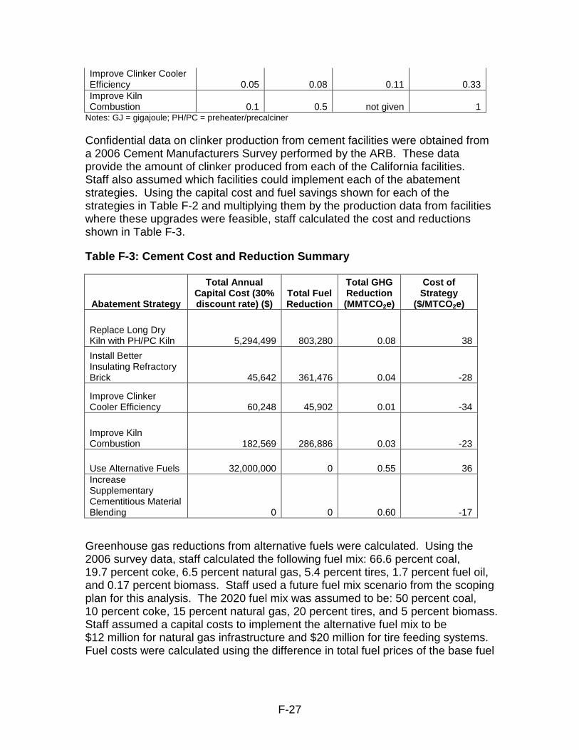
Improve Clinker Cooler Efficiency 0.05 0.08 0.11 0.33 Improve Kiln Combustion 0.1 0.5 not given 1
Notes: GJ = gigajoule; PH/PC = preheater/precalciner
Confidential data on clinker production from cement facilities were obtained from a 2006 Cement Manufacturers Survey performed by the ARB. These data provide the amount of clinker produced from each of the California facilities. Staff also assumed which facilities could implement each of the abatement strategies. Using the capital cost and fuel savings shown for each of the strategies in Table F-2 and multiplying them by the production data from facilities where these upgrades were feasible, staff calculated the cost and reductions shown in Table F-3.
Table F-3: Cement Cost and Reduction Summary
Abatement Strategy
Total Annual Capital Cost (30% discount rate) ($)
Total Fuel Reduction
Total GHG Reduction (MMTCO2e)
Cost of Strategy
($/MTCO2e)
Replace Long Dry Kiln with PH/PC Kiln 5,294,499 803,280 0.08 38
Install Better Insulating Refractory Brick 45,642 361,476 0.04 -28
Improve Clinker Cooler Efficiency 60,248 45,902 0.01 -34
Improve Kiln Combustion 182,569 286,886 0.03 -23
Use Alternative Fuels 32,000,000 0 0.55 36 Increase Supplementary Cementitious Material Blending 0 0 0.60 -17
Greenhouse gas reductions from alternative fuels were calculated. Using the 2006 survey data, staff calculated the following fuel mix: 66.6 percent coal, 19.7 percent coke, 6.5 percent natural gas, 5.4 percent tires, 1.7 percent fuel oil, and 0.17 percent biomass. Staff used a future fuel mix scenario from the scoping plan for this analysis. The 2020 fuel mix was assumed to be: 50 percent coal, 10 percent coke, 15 percent natural gas, 20 percent tires, and 5 percent biomass. Staff assumed a capital costs to implement the alternative fuel mix to be $12 million for natural gas infrastructure and $20 million for tire feeding systems. Fuel costs were calculated using the difference in total fuel prices of the base fuel
F-28
mix and the future fuel mix. GHG reductions were calculated using the difference in total GHG emissions from using the base fuel mix and the future fuel mix.
For supplementary cementitious material (SCM) blending, staff assumed the current percent of SCM blending to be 8 percent.53 Staff assumed a future blending mix of 15 percent SCM in 2020. Staff used 15 percent to match the current Caltrans blending standards. Staff assumed no capital cost for SCM blending. Staff used a savings of $20 per ton of cement.53 From the 2006 survey, 11.6 million tons of cement were produced and emissions were 10 MMTCO2e. Thus, the intensity of producing cement is 1.16 MMTCO2e/million tons of cement. Staff assumed a 2020 emissions forecast from the cement sector to be 8.6 MMTCO2e.54 Dividing the 2020 emissions quantity by the emissions intensity of cement obtains 7.4 million tons of cement produced in 2020. Blending an additional 7 percent of SCMs will save $10.4 million. It is assumed that there are no GHG emissions associated with SCM blending because SCM are mostly fly ash produced as a by-product of burning coal. Thus, blending an additional 7 percent of SCM will result in a 7 percent reduction from the business-as-usual (BAU) scenario, 0.6 MMTCO2e. Thus, the cost per ton is the ratio of total cost savings and total emissions reductions, -$17/metric ton.
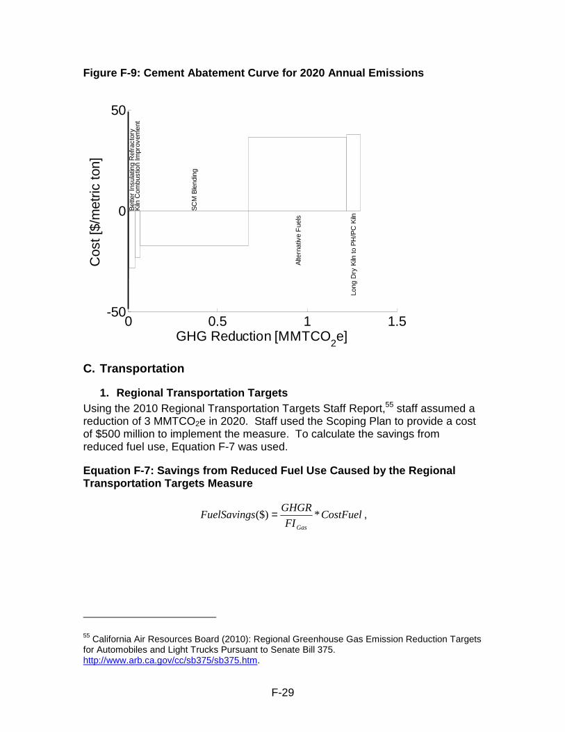
Cement greenhouse gas emission reductions strategies and associated costs are shown below in Figure F-9.
53 Personal communication with Headwaters Resources. 54 The 2020 baseline forecast can be found at ARB’s “Greenhouse Gas Inventory - 2020 Forecast” webpage: http://www.arb.ca.gov/cc/inventory/data/forecast.htm.
F-29
Figure F-9: Cement Abatement Curve for 2020 Annual Emissions
0 0.5 1 1.5-50
0
50C
ost [
$/m
etric
ton]
GHG Reduction [MMTCO2e]
Bet
ter
Insu
latin
g R
efra
ctor
yK
iln C
ombu
stio
n Im
prov
emen
t
SC
M B
lend
ing
Alte
rnat
ive
Fue
ls
Long
Dry
Kiln
to P
H/P
C K
iln
C. Transportation
1. Regional Transportation Targets Using the 2010 Regional Transportation Targets Staff Report,55 staff assumed a reduction of 3 MMTCO2e in 2020. Staff used the Scoping Plan to provide a cost of $500 million to implement the measure. To calculate the savings from reduced fuel use, Equation F-7 was used.
Equation F-7: Savings from Reduced Fuel Use Caused by the Regional Transportation Targets Measure
CostFuelFI
GHGRsFuelSaving
Gas
*($) = ,
55 California Air Resources Board (2010): Regional Greenhouse Gas Emission Reduction Targets for Automobiles and Light Trucks Pursuant to Senate Bill 375. http://www.arb.ca.gov/cc/sb375/sb375.htm.
F-30
where GHGR is the GHG reduction of the strategy (in MMTCO2e), FI is the fuel intensity of gasoline (0.00894 MTCO2e/gallon),6 and CostFuel is the cost of gasoline ($3.36 per gallon price of fuel).56. The savings are estimated to be $1,128 million (M). Thus, the cost per metric ton is $500M (cost of the program) minus $1,128M (savings from the program), all divided by 3 MMTCO2e = -$209/metric ton.
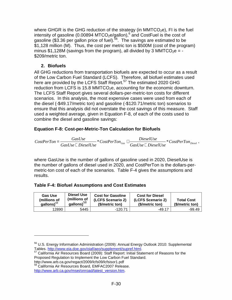
2. Biofuels All GHG reductions from transportation biofuels are expected to occur as a result of the Low Carbon Fuel Standard (LCFS). Therefore, all biofuel estimates used here are provided by the LCFS Staff Report.57 The estimated 2020 GHG reduction from LCFS is 15.8 MMTCO2e, accounting for the economic downturn. The LCFS Staff Report gives several dollars-per-metric-ton costs for different scenarios. In this analysis, the most expensive cases were used from each of the diesel (-$49.17/metric ton) and gasoline (-$120.71/metric ton) scenarios to ensure that this analysis did not overstate the cost savings of this measure. Staff used a weighted average, given in Equation F-8, of each of the costs used to combine the diesel and gasoline savings:
Equation F-8: Cost-per-Metric-Ton Calculation for Biofuels
DieselGas CostPerTonDieselUseGasUse
DieselUseCostPerTon
DieselUseGasUse
GasUseCostPerTon **
++
+= ,
where GasUse is the number of gallons of gasoline used in 2020, DieselUse is the number of gallons of diesel used in 2020, and CostPerTon is the dollars-per-metric-ton cost of each of the scenarios. Table F-4 gives the assumptions and results.
Table F-4: Biofuel Assumptions and Cost Estimates
Gas Use (millions of gallons)58
Diesel Use (millions of gallons)58
Cost for Gasoline (LCFS Scenario 2)
($/metric ton)
Cost for Diesel (LCFS Scenario 2)
($/metric ton) Total Cost
($/metric ton) 12890 5445 -120.71 -49.17 -99.49
56 U.S. Energy Information Administration (2009): Annual Energy Outlook 2010: Supplemental Tables. http://www.eia.doe.gov/oiaf/aeo/supplement/supref.html. 57 California Air Resources Board (2009): Staff Report: Initial Statement of Reasons for the Proposed Regulation to Implement the Low Carbon Fuel Standard. http://www.arb.ca.gov/regact/2009/lcfs09/lcfsisor1.pdf 58 California Air Resources Board, EMFAC2007 Release. http://www.arb.ca.gov/msei/onroad/latest_version.htm.
F-31
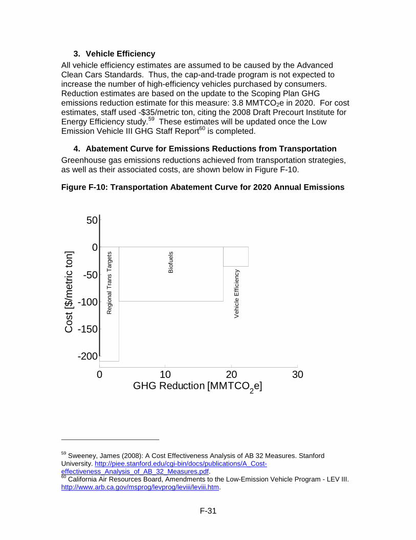
3. Vehicle Efficiency All vehicle efficiency estimates are assumed to be caused by the Advanced Clean Cars Standards. Thus, the cap-and-trade program is not expected to increase the number of high-efficiency vehicles purchased by consumers. Reduction estimates are based on the update to the Scoping Plan GHG emissions reduction estimate for this measure: 3.8 MMTCO2e in 2020. For cost estimates, staff used -$35/metric ton, citing the 2008 Draft Precourt Institute for Energy Efficiency study.59 These estimates will be updated once the Low Emission Vehicle III GHG Staff Report60 is completed.
4. Abatement Curve for Emissions Reductions from Transportation Greenhouse gas emissions reductions achieved from transportation strategies, as well as their associated costs, are shown below in Figure F-10.
Figure F-10: Transportation Abatement Curve for 2020 Annual Emissions
0 10 20 30
-200
-150
-100
-50
0
50
Cos
t [$/
met
ric to
n]
GHG Reduction [MMTCO2e]
Reg
iona
l Tra
ns T
arge
ts
Bio
fuel
s
Veh
icle
Eff
icie
ncy
59 Sweeney, James (2008): A Cost Effectiveness Analysis of AB 32 Measures. Stanford University. http://piee.stanford.edu/cgi-bin/docs/publications/A_Cost-effectiveness_Analysis_of_AB_32_Measures.pdf. 60 California Air Resources Board, Amendments to the Low-Emission Vehicle Program - LEV III. http://www.arb.ca.gov/msprog/levprog/leviii/leviii.htm.
F-32
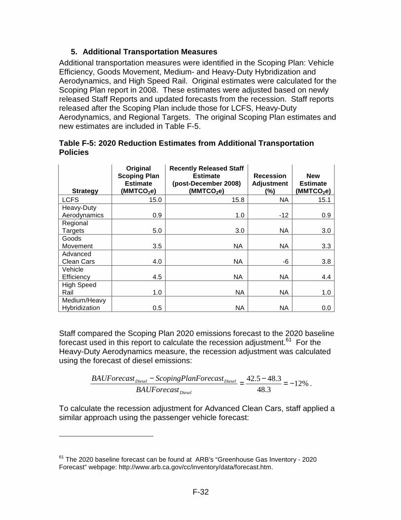
5. Additional Transportation Measures Additional transportation measures were identified in the Scoping Plan: Vehicle Efficiency, Goods Movement, Medium- and Heavy-Duty Hybridization and Aerodynamics, and High Speed Rail. Original estimates were calculated for the Scoping Plan report in 2008. These estimates were adjusted based on newly released Staff Reports and updated forecasts from the recession. Staff reports released after the Scoping Plan include those for LCFS, Heavy-Duty Aerodynamics, and Regional Targets. The original Scoping Plan estimates and new estimates are included in Table F-5.
Table F-5: 2020 Reduction Estimates from Additional Transportation Policies
Strategy
Original Scoping Plan
Estimate (MMTCO2e)
Recently Released Staff Estimate
(post-December 2008) (MMTCO2e)
Recession Adjustment
(%)
New Estimate
(MMTCO2e) LCFS 15.0 15.8 NA 15.1 Heavy-Duty Aerodynamics 0.9 1.0 -12 0.9 Regional Targets 5.0 3.0 NA 3.0 Goods Movement 3.5 NA NA 3.3 Advanced Clean Cars 4.0 NA -6 3.8 Vehicle Efficiency 4.5 NA NA 4.4 High Speed Rail 1.0 NA NA 1.0 Medium/Heavy Hybridization 0.5 NA NA 0.0
Staff compared the Scoping Plan 2020 emissions forecast to the 2020 baseline forecast used in this report to calculate the recession adjustment.61 For the Heavy-Duty Aerodynamics measure, the recession adjustment was calculated using the forecast of diesel emissions:
%123.48
3.485.42 −=−=−
Diesel
DieselDiesel
tBAUForecas
nForecastScopingPlatBAUForecas.
To calculate the recession adjustment for Advanced Clean Cars, staff applied a similar approach using the passenger vehicle forecast:
61 The 2020 baseline forecast can be found at ARB’s “Greenhouse Gas Inventory - 2020 Forecast” webpage: http://www.arb.ca.gov/cc/inventory/data/forecast.htm.
F-33
%7.58.160
8.1606.151 =−=−
ehiclesPassengerV
ehiclesPassengerVehiclesPassengerV
tBAUForecas
nForecastScopingPlatBAUForecas.
For the Regional Targets and High Speed Rail measures, no adjustment from the economic downturn was assumed. For Vehicle Efficiency and Goods Movement, staff assumed reductions of 4.4 and 3.3 MMTCO2e, respectively.6
D. Power Generation
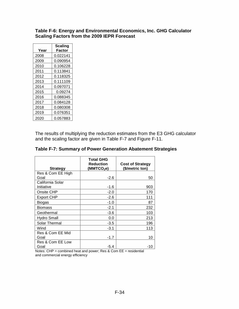
1. Renewable Energy, Combined Heat and Power The power generation abatement curve was created using the E3 GHG calculator.62 The accelerated policy case (33 percent Renewable Electricity Standard, high adoption of energy efficiency) was run using the E3 GHG calculator. The curve was also run with low, medium, and high energy-efficiency goals63 to calculate the marginal GHG reduction and cost for each of the goals. The abatement curve from the model was then scaled linearly with the new 2009 Integrated Energy Policy Report (IEPR)64 electricity demand forecast. The scaling factor is the quotient of the E3 GHG electricity forecast and 2009 IEPR forecast. Table F-6 shows the results.
62 Energy and Environmental Economics, Inc. (2010): Greenhouse Gas Calculator for the California Electricity Sector. http://www.ethree.com/documents/GHG%203.11.10/GHG%20Calculator%20version%203b_Final_to_Post_March2010.zip. 63 CPUC Rulemaking 06-04-010, Decision 08-07-047, “Decision Adopting Interim Energy Efficiency Savings Goals for 2012 through 2020, and Defining Energy Efficiency Savings Goals for 2009 through 2011,” August 1, 2008. 64 California Energy Commission (2009): Integrated Energy Policy Report, Final Commission Report. CEC -100-2009-003-CMF. http://www.energy.ca.gov/2009publications/CEC-100-2009-003/CEC-100-2009-003-CMF.PDF (accessed October 25, 2010).
F-34
Table F-6: Energy and Environmental Economics, Inc. GHG Calculator Scaling Factors from the 2009 IEPR Forecast
Year Scaling Factor
2008 0.022141 2009 0.090954 2010 0.106228 2011 0.113841 2012 0.118325 2013 0.111109 2014 0.097071 2015 0.09274 2016 0.088345 2017 0.084128 2018 0.080308 2019 0.076351
2020 0.057883
The results of multiplying the reduction estimates from the E3 GHG calculator and the scaling factor are given in Table F-7 and Figure F-11.
Table F-7: Summary of Power Generation Abatement Strategies
Strategy
Total GHG Reduction (MMTCO2e)
Cost of Strategy ($/metric ton)
Res & Com EE High Goal -2.6 50 California Solar Initiative -1.6 903 Onsite CHP -2.0 170 Export CHP -2.6 111 Biogas -1.0 87 Biomass -2.1 232 Geothermal -3.6 103 Hydro Small 0.0 213 Solar Thermal -3.5 196 Wind -3.1 113 Res & Com EE Mid Goal -1.7 10 Res & Com EE Low Goal -5.4 -10
Notes: CHP = combined heat and power; Res & Com EE = residential and commercial energy efficiency
F-35
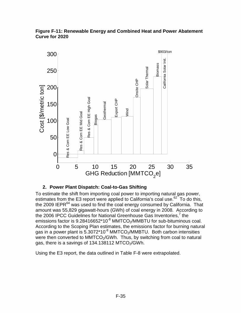
Figure F-11: Renewable Energy and Combined Heat and Power Abatement Curve for 2020
0 5 10 15 20 25 30 35
0
50
100
150
200
250
300
Cos
t [$/
met
ric to
n]
GHG Reduction [MMTCO2e]
Res
& C
om E
E L
ow G
oal
Res
& C
om E
E M
id G
oal
Res
& C
om E
E H
igh
Goa
l
Bio
gas
Geo
ther
mal
Exp
ort
CH
P
Win
d
Ons
ite C
HP
Sol
ar T
herm
al
Bio
mas
s
Cal
iforn
ia S
olar
Ini
t.
$903/ton
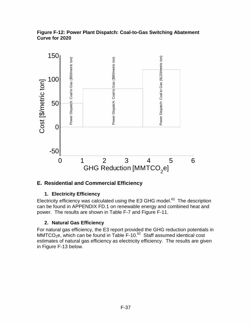
2. Power Plant Dispatch: Coal-to-Gas Shifting To estimate the shift from importing coal power to importing natural gas power, estimates from the E3 report were applied to California’s coal use.62 To do this, the 2009 IEPR64 was used to find the coal energy consumed by California. That amount was 55,829 gigawatt-hours (GWh) of coal energy in 2008. According to the 2006 IPCC Guidelines for National Greenhouse Gas Inventories,7 the emissions factor is 9.28416652*10-8 MMTCO2/MMBTU for sub-bituminous coal. According to the Scoping Plan estimates, the emissions factor for burning natural gas in a power plant is 5.3072*10-8 MMTCO2/MMBTU. Both carbon intensities were then converted to MMTCO2/GWh. Thus, by switching from coal to natural gas, there is a savings of 134.138112 MTCO2/GWh.
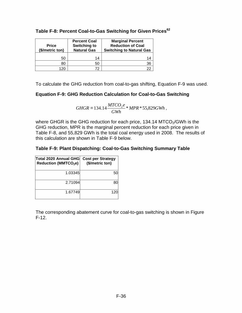
Using the E3 report, the data outlined in Table F-8 were extrapolated.
F-36
Table F-8: Percent Coal-to-Gas Switching for Given Prices62
Price ($/metric ton)
Percent Coal Switching to Natural Gas
Marginal Percent Reduction of Coal
Switching to Natural Gas
50 14 14 80 50 36
120 72 22
To calculate the GHG reduction from coal-to-gas shifting, Equation F-9 was used.
Equation F-9: GHG Reduction Calculation for Coal-to-Gas Switching
GWhMPRGWh
eMTCOGHGR 829,55**14.134 2= ,
where GHGR is the GHG reduction for each price, 134.14 MTCO2/GWh is the GHG reduction, MPR is the marginal percent reduction for each price given in Table F-8, and 55,829 GWh is the total coal energy used in 2008. The results of this calculation are shown in Table F-9 below.
Table F-9: Plant Dispatching: Coal-to-Gas Switching Summary Table
Total 2020 Annual GHG Reduction (MMTCO2e)
Cost per Strategy ($/metric ton)
1.03345 50
2.71094 80
1.67749 120
The corresponding abatement curve for coal-to-gas switching is shown in Figure F-12.
F-37
Figure F-12: Power Plant Dispatch: Coal-to-Gas Switching Abatement Curve for 2020
0 1 2 3 4 5 6-50
0
50
100
150
Cos
t [$/
met
ric to
n]
GHG Reduction [MMTCO2e]
Pow
er D
ispa
tch:
Coa
l to
Gas
($5
0/m
etric
ton)
Pow
er D
ispa
tch:
Coa
l to
Gas
($8
0/m
etric
ton)
Pow
er D
ispa
tch:
Coa
l to
Gas
($1
20/m
etric
ton)
E. Residential and Commercial Efficiency
1. Electricity Efficiency Electricity efficiency was calculated using the E3 GHG model.62 The description can be found in APPENDIX FD.1 on renewable energy and combined heat and power. The results are shown in Table F-7 and Figure F-11.
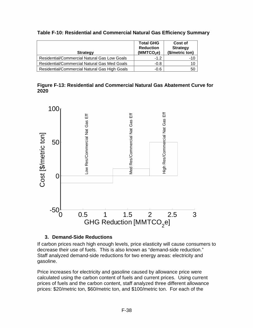
2. Natural Gas Efficiency For natural gas efficiency, the E3 report provided the GHG reduction potentials in MMTCO2e, which can be found in Table F-10.62 Staff assumed identical cost estimates of natural gas efficiency as electricity efficiency. The results are given in Figure F-13 below.
F-38
Table F-10: Residential and Commercial Natural Gas Efficiency Summary
Strategy
Total GHG Reduction (MMTCO2e)
Cost of Strategy
($/metric ton) Residential/Commercial Natural Gas Low Goals -1.2 -10 Residential/Commercial Natural Gas Med Goals -0.8 10 Residential/Commercial Natural Gas High Goals -0.6 50
Figure F-13: Residential and Commercial Natural Gas Abatement Curve for 2020
0 0.5 1 1.5 2 2.5 3-50
0
50
100
Cos
t [$/
met
ric to
n]
GHG Reduction [MMTCO2e]
Low
Res
/Com
mer
cial
Nat
Gas
Eff
Med
Res
/Com
mer
cial
Nat
Gas
Eff
Hig
h R
es/C
omm
erci
al N
at G
as E
ff
3. Demand-Side Reductions If carbon prices reach high enough levels, price elasticity will cause consumers to decrease their use of fuels. This is also known as “demand-side reduction.” Staff analyzed demand-side reductions for two energy areas: electricity and gasoline.
Price increases for electricity and gasoline caused by allowance price were calculated using the carbon content of fuels and current prices. Using current prices of fuels and the carbon content, staff analyzed three different allowance prices: $20/metric ton, $60/metric ton, and $100/metric ton. For each of the
F-39
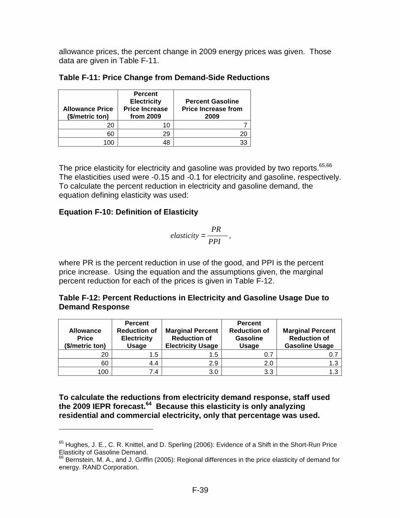
allowance prices, the percent change in 2009 energy prices was given. Those data are given in Table F-11.
Table F-11: Price Change from Demand-Side Reductions
Allowance Price ($/metric ton)
Percent Electricity
Price Increase from 2009
Percent Gasoline Price Increase from
2009 20 10 7 60 29 20
100 48 33
The price elasticity for electricity and gasoline was provided by two reports.65,66 The elasticities used were -0.15 and -0.1 for electricity and gasoline, respectively. To calculate the percent reduction in electricity and gasoline demand, the equation defining elasticity was used:
Equation F-10: Definition of Elasticity
PPI
PRelasticity = ,
where PR is the percent reduction in use of the good, and PPI is the percent price increase. Using the equation and the assumptions given, the marginal percent reduction for each of the prices is given in Table F-12.
Table F-12: Percent Reductions in Electricity and Gasoline Usage Due to Demand Response
Allowance Price
($/metric ton)
Percent Reduction of
Electricity Usage
Marginal Percent Reduction of
Electricity Usage
Percent Reduction of
Gasoline Usage
Marginal Percent Reduction of
Gasoline Usage 20 1.5 1.5 0.7 0.7 60 4.4 2.9 2.0 1.3
100 7.4 3.0 3.3 1.3
To calculate the reductions from electricity demand response, staff used the 2009 IEPR forecast.64 Because this elasticity is only analyzing residential and commercial electricity, only that percentage was used.
65 Hughes, J. E., C. R. Knittel, and D. Sperling (2006): Evidence of a Shift in the Short-Run Price Elasticity of Gasoline Demand. 66 Bernstein, M. A., and J. Griffin (2005): Regional differences in the price elasticity of demand for energy. RAND Corporation.
F-40
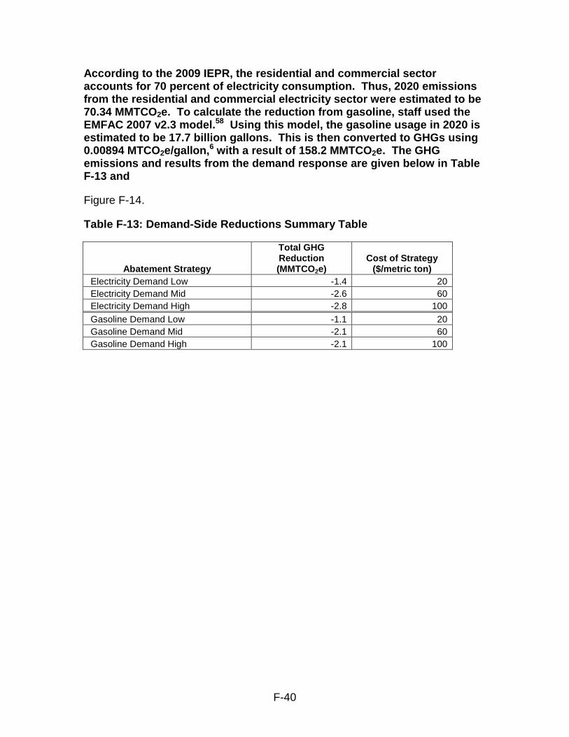
According to the 2009 IEPR, the residential and commercial sector accounts for 70 percent of electricity consumption. Thus, 2020 emissions from the residential and commercial electricity sector were estimated to be 70.34 MMTCO2e. To calculate the reduction from gasoline, staff used the EMFAC 2007 v2.3 model.58 Using this model, the gasoline usage in 2020 is estimated to be 17.7 billion gallons. This is then converted to GHGs using 0.00894 MTCO2e/gallon,6 with a result of 158.2 MMTCO2e. The GHG emissions and results from the demand response are given below in Table F-13 and
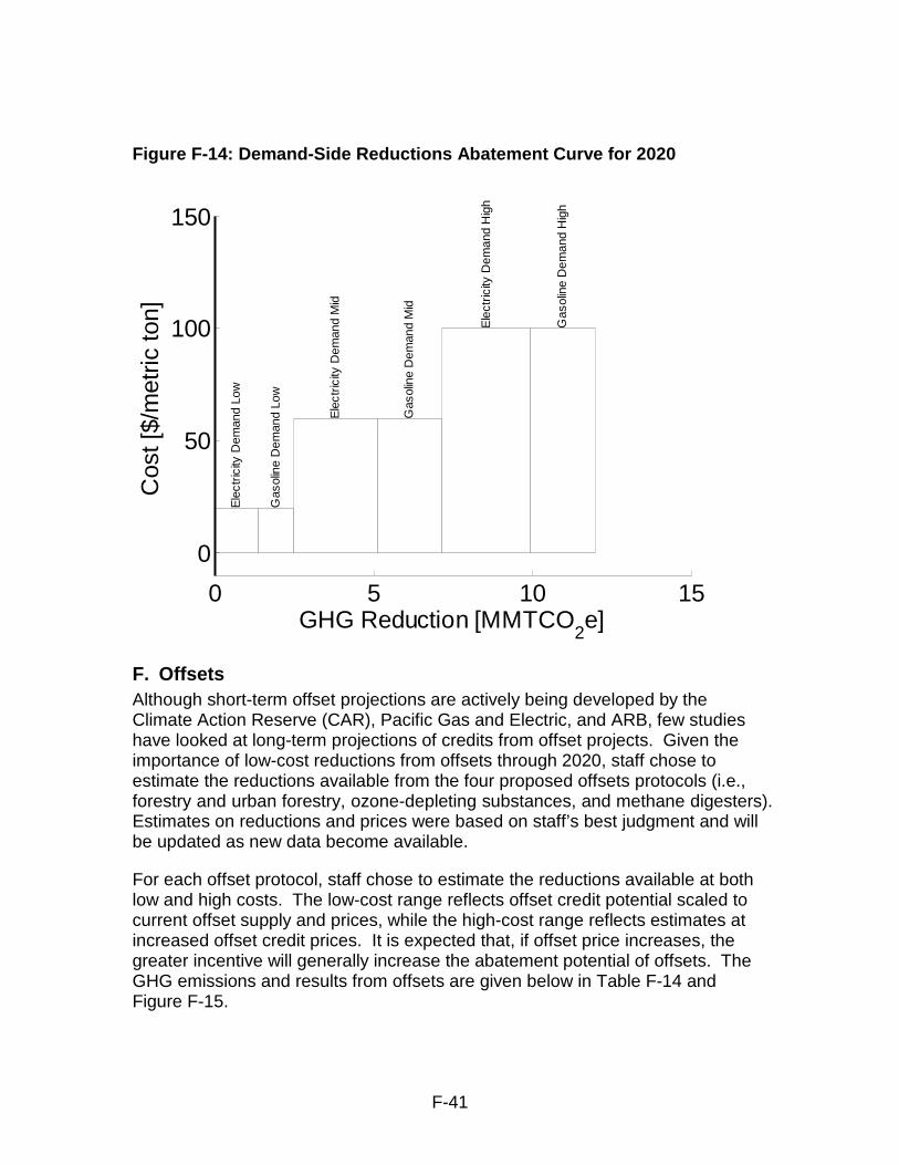
Figure F-14.
Table F-13: Demand-Side Reductions Summary Table
Abatement Strategy
Total GHG Reduction (MMTCO2e)
Cost of Strategy ($/metric ton)
Electricity Demand Low -1.4 20 Electricity Demand Mid -2.6 60 Electricity Demand High -2.8 100 Gasoline Demand Low -1.1 20 Gasoline Demand Mid -2.1 60 Gasoline Demand High -2.1 100
F-41
Figure F-14: Demand-Side Reductions Abatement Curve for 2020
0 5 10 15
0
50
100
150
Cos
t [$/
met
ric to
n]
GHG Reduction [MMTCO2e]
Ele
ctric
ity D
eman
d Lo
w
Gas
olin
e D
eman
d Lo
w
Ele
ctric
ity D
eman
d M
id
Gas
olin
e D
eman
d M
id
Ele
ctric
ity D
eman
d H
igh
Gas
olin
e D
eman
d H
igh
F. Offsets Although short-term offset projections are actively being developed by the Climate Action Reserve (CAR), Pacific Gas and Electric, and ARB, few studies have looked at long-term projections of credits from offset projects. Given the importance of low-cost reductions from offsets through 2020, staff chose to estimate the reductions available from the four proposed offsets protocols (i.e., forestry and urban forestry, ozone-depleting substances, and methane digesters). Estimates on reductions and prices were based on staff’s best judgment and will be updated as new data become available.
For each offset protocol, staff chose to estimate the reductions available at both low and high costs. The low-cost range reflects offset credit potential scaled to current offset supply and prices, while the high-cost range reflects estimates at increased offset credit prices. It is expected that, if offset price increases, the greater incentive will generally increase the abatement potential of offsets. The GHG emissions and results from offsets are given below in Table F-14 and Figure F-15.
F-42
For more information on the offsets protocols being developed, see Staff Report Part I, Volume I, Chapter III: Overview of the Compliance Offset Program.
1. Forestry67 The number of forestry offset credits currently issued by CAR is approximately 700,000. Most of these credits are from projects within California and sell for a price of approximately $4 per metric ton. With increased market assurance of a cap-and-trade program, it is expected that the number of credits would increase and that out-of-state projects would be incentivized. Staff estimated that 5 MMTCO2e of offsets would be generated in 2020, and assumed a relatively high price of $8/metric ton. If allowance prices were to increase to $20/metric ton, staff assumed a widespread investment in forestry offsets; at this price, staff estimate that the number of offsets generated in 2020 would be 10 MMTCO2e.
Because the forestry estimates contain a high degree of uncertainty, staff will continue to update estimates of long-term forestry offset supply.
2. Ozone-Depleting Substances At current $4/metric ton prices, there are several large ozone-depleting substances (ODS) projects listed by CAR. The number of ODS projects is expected to increase with implementation of the proposed cap-and-trade program. In the low-price range, refrigerants are expected to be the primary compound destroyed. The most common of these chemicals is CFC-12. Based on CFC sales,68 the annual reduction potential is 8.8 MMTCO2e at an estimated price range estimated of $1–$10/metric ton. To err on the conservative side, staff used a price of $10 per metric ton.
At higher costs, ODS offset projects would likely involve destroying building insulation and appliance foams. These materials have a lower GHG reduction potential than refrigerant compounds because of their lower quantities. Staff estimated reductions of 1 MMTCO2e at $9 to $28/metric ton, within which staff chose a conservative price of $25.
3. Methane Digesters Offset projects for livestock methane capture and destruction exist both in and outside California. The number of California projects is limited because the intent to combust methane may trigger requirements for new or revised NOx permits. Outside of California, there are many more methane digester projects because of less stringent NOx standards. At lot prices, the number of credits generated annually is not expected to increase due to difficultly permitting. Staff assumed that methane digesters have an annual reduction potential of 500,000 MTCO2e in 2020 at a price of $8/metric ton.
67 Includes both forestry and urban forestry. 68 http://unfccc.int/files/methods_and_science/other_methodological_issues/ interactions_with_ozone_layer/application/pdf/cfc12sales00.pdf
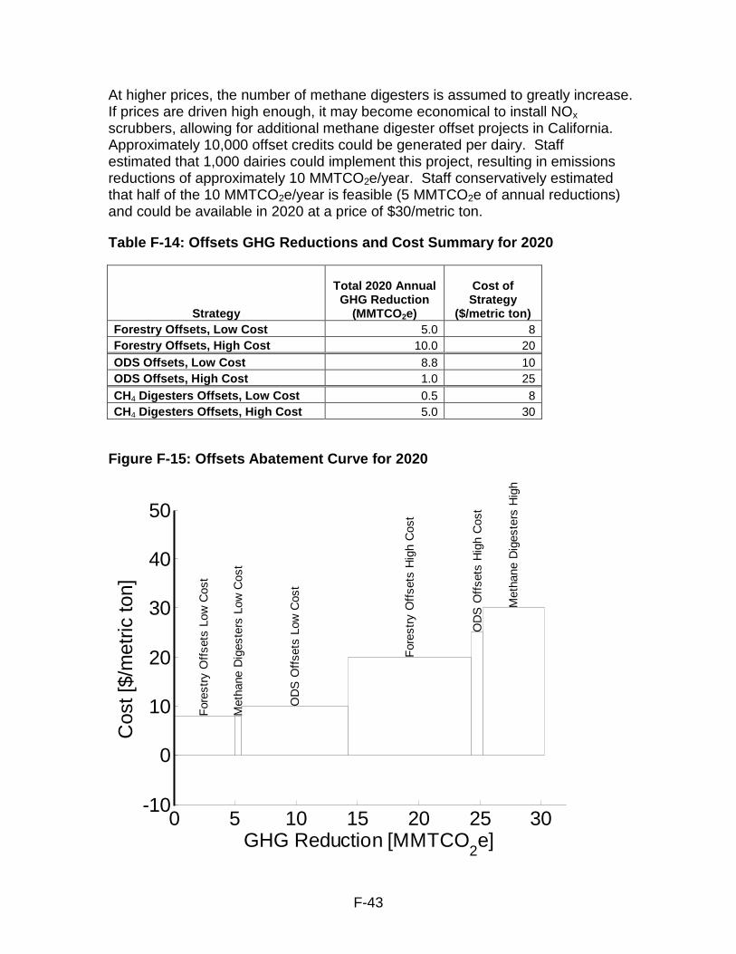
F-43
At higher prices, the number of methane digesters is assumed to greatly increase. If prices are driven high enough, it may become economical to install NOx scrubbers, allowing for additional methane digester offset projects in California. Approximately 10,000 offset credits could be generated per dairy. Staff estimated that 1,000 dairies could implement this project, resulting in emissions reductions of approximately 10 MMTCO2e/year. Staff conservatively estimated that half of the 10 MMTCO2e/year is feasible (5 MMTCO2e of annual reductions) and could be available in 2020 at a price of $30/metric ton.
Table F-14: Offsets GHG Reductions and Cost Summary for 2020
Strategy
Total 2020 Annual GHG Reduction
(MMTCO2e)
Cost of Strategy
($/metric ton) Forestry Offsets, Low Cost 5.0 8 Forestry Offsets, High Cost 10.0 20 ODS Offsets, Low Cost 8.8 10 ODS Offsets, High Cost 1.0 25 CH4 Digesters Offsets, Low Cost 0.5 8 CH4 Digesters Offsets, High Cost 5.0 30
Figure F-15: Offsets Abatement Curve for 2020
0 5 10 15 20 25 30-10
0
10
20
30
40
50
Cos
t [$/
met
ric to
n]
GHG Reduction [MMTCO2e]
For
estr
y O
ffse
ts L
ow C
ost
Met
hane
Dig
este
rs L
ow C
ost
OD
S O
ffse
ts L
ow C
ost
For
estr
y O
ffse
ts H
igh
Cos
t
OD
S O
ffse
ts H
igh
Cos
t
Met
hane
Dig
este
rs H
igh
Cos
t

F-44

F-45
This Page Intentionally Left Blank