Appendix E: Systems of Inequalities - Cengage · E1 The Graph of an Inequality The statements 3x − 2y < 6 and 2x2 + 3y2 ≥ 6 are inequalities in two variables. An ordered pair

E1

The Graph of an InequalityThe statements 3x − 2y < 6 and 2x2 + 3y2 ≥ 6 are inequalities in two variables. An ordered pair (a, b) is a solution of an inequality in x and y for which the inequality is true when a and b are substituted for x and y, respectively. The graph of an inequality is the collection of all solutions of the inequality. To sketch the graph of an inequality, begin by sketching the graph of the corresponding equation. The graph of the equation will normally separate the plane into two or more regions. In each such region, one of the following must be true.

1. All points in the region are solutions of the inequality.

2. No point in the region is a solution of the inequality.

So, you can determine whether the points in an entire region satisfy the inequality by simply testing one point in the region.

Sketching the Graph of an Inequality in Two Variables

1. Replace the inequality sign with an equal sign and sketch the graph of the corresponding equation. Use a dashed line for < or > and a solid line for ≤ or ≥. (A dashed line means that all points on the line or curve are not solutions of the inequality. A solid line means that all points on the line or curve are solutions of the inequality.)

2. Test one point in each of the regions formed by the graph in Step 1. When the point satisfies the inequality, shade the entire region to denote that every point in the region satisfies the inequality.

EXAMPLE 1 Sketching the Graph of an Inequality

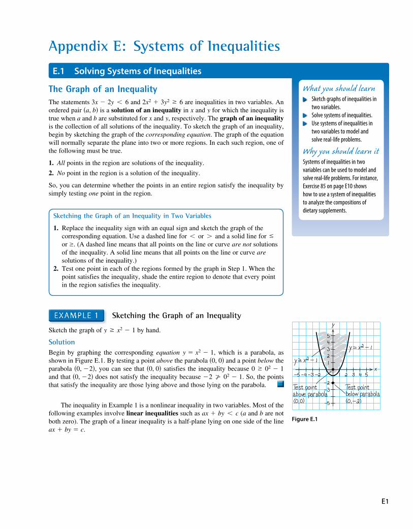
Sketch the graph of y ≥ x2 − 1 by hand.

SolutionBegin by graphing the corresponding equation y = x2 − 1, which is a parabola, as shown in Figure E.1. By testing a point above the parabola (0, 0) and a point below the parabola (0, −2), you can see that (0, 0) satisfies the inequality because 0 ≥ 02 − 1 and that (0, −2) does not satisfy the inequality because −2 >∕ 02 − 1. So, the points that satisfy the inequality are those lying above and those lying on the parabola.

The inequality in Example 1 is a nonlinear inequality in two variables. Most of the following examples involve linear inequalities such as ax + by < c (a and b are not both zero). The graph of a linear inequality is a half-plane lying on one side of the line ax + by = c.

E.1 Solving Systems of Inequalities

What you should learn Sketch graphs of inequalities in

two variables. Solve systems of inequalities. Use systems of inequalities in

two variables to model and solve real-life problems.

Why you should learn itSystems of inequalities in two variables can be used to model and solve real-life problems. For instance, Exercise 85 on page E10 shows how to use a system of inequalities to analyze the compositions of dietary supplements.

Appendix E: Systems of Inequalities

Figure E.1

E2 Appendix E Systems of Inequalities

EXAMPLE 2 Sketching the Graphs of Linear Inequalities

Sketch the graph of each linear inequality.

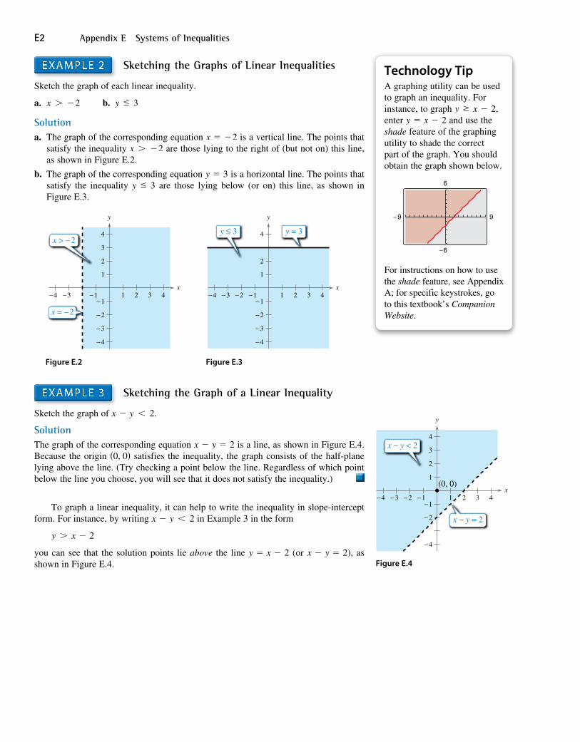
a. x > −2 b. y ≤ 3

Solutiona. The graph of the corresponding equation x = −2 is a vertical line. The points that

satisfy the inequality x > −2 are those lying to the right of (but not on) this line, as shown in Figure E.2.

b. The graph of the corresponding equation y = 3 is a horizontal line. The points that satisfy the inequality y ≤ 3 are those lying below (or on) this line, as shown in Figure E.3.

y

−1−3−4 1 2 3 4−1

−2

−3

−4

1

2

3

4

x

x > −2

x = −2

y

−1−2−3−4 1 2 3 4−1

−2

−3

−4

1

2

4

x

y ≤ 3 y = 3

Figure E.2 Figure E.3

EXAMPLE 3 Sketching the Graph of a Linear Inequality

Sketch the graph of x − y < 2.

SolutionThe graph of the corresponding equation x − y = 2 is a line, as shown in Figure E.4. Because the origin (0, 0) satisfies the inequality, the graph consists of the half-plane lying above the line. (Try checking a point below the line. Regardless of which point below the line you choose, you will see that it does not satisfy the inequality.)

To graph a linear inequality, it can help to write the inequality in slope-intercept form. For instance, by writing x − y < 2 in Example 3 in the form

y > x − 2

you can see that the solution points lie above the line y = x − 2 (or x − y = 2), as shown in Figure E.4.

Technology TipA graphing utility can be used to graph an inequality. For instance, to graph y ≥ x − 2, enter y = x − 2 and use the shade feature of the graphing utility to shade the correct part of the graph. You should obtain the graph shown below.

−6

−9 9

6

For instructions on how to use the shade feature, see Appendix A; for specific keystrokes, go to this textbook’s Companion Website.

Figure E.4

y

−1−2−3−4 1 2 3 4−1

−2

−4

1

2

3

4

x(0, 0)

x − y = 2

x − y < 2

Appendix E.1 Solving Systems of Inequalities E3

Systems of InequalitiesMany practical problems in business, science, and engineering involve systems of linear inequalities. A solution of a system of inequalities in x and y is a point (x, y) that satisfies each inequality in the system.

To sketch the graph of a system of inequalities in two variables, first sketch the graph of each individual inequality (on the same coordinate system) and then find the region that is common to every graph in the system. For systems of linear inequalities, it is helpful to find the vertices of the solution region.

EXAMPLE 4 Solving a System of Inequalities

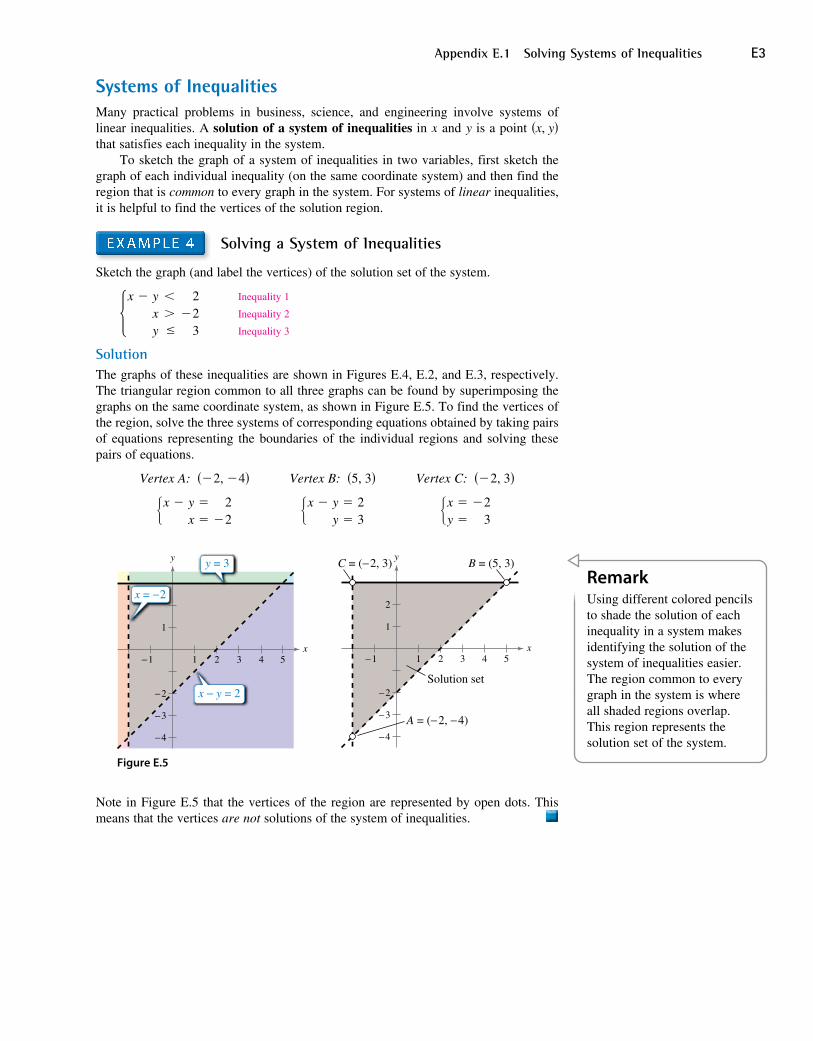
Sketch the graph (and label the vertices) of the solution set of the system.

{x − yxy

<>≤

2−2

3

Inequality 1

Inequality 2

Inequality 3

SolutionThe graphs of these inequalities are shown in Figures E.4, E.2, and E.3, respectively. The triangular region common to all three graphs can be found by superimposing the graphs on the same coordinate system, as shown in Figure E.5. To find the vertices of the region, solve the three systems of corresponding equations obtained by taking pairs of equations representing the boundaries of the individual regions and solving these pairs of equations.

Vertex A: (−2, −4) Vertex B: (5, 3) Vertex C: (−2, 3)

{x − yx==

2−2

{x − yy==

23 {xy =

=−2

3

−1 1 2 3 4 5

1

−2

−3

−4

y

x

x − y = 2

y = 3

x = −2

2

C = (−2, 3)

A = (−2, −4)

B = (5, 3)

Solution set

y

x−1 1 2 3 4 5

1

−2

−3

−4

Figure E.5

Note in Figure E.5 that the vertices of the region are represented by open dots. This means that the vertices are not solutions of the system of inequalities.

RemarkUsing different colored pencils to shade the solution of each inequality in a system makes identifying the solution of the system of inequalities easier. The region common to every graph in the system is where all shaded regions overlap. This region represents the solution set of the system.


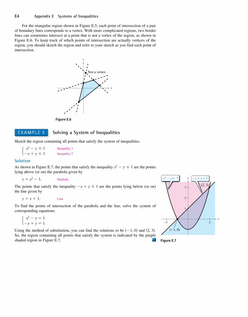
For the triangular region shown in Figure E.5, each point of intersection of a pair of boundary lines corresponds to a vertex. With more complicated regions, two border lines can sometimes intersect at a point that is not a vertex of the region, as shown in Figure E.6. To keep track of which points of intersection are actually vertices of the region, you should sketch the region and refer to your sketch as you find each point of intersection.

Not a vertex

y

x

Figure E.6

EXAMPLE 5 Solving a System of Inequalities

Sketch the region containing all points that satisfy the system of inequalities.

{ x2 − y−x + y

≤≤

11

Inequality 1

Inequality 2

SolutionAs shown in Figure E.7, the points that satisfy the inequality x2 − y ≤ 1 are the points lying above (or on) the parabola given by

y = x2 − 1. Parabola

The points that satisfy the inequality −x + y ≤ 1 are the points lying below (or on) the line given by

y = x + 1. Line

To find the points of intersection of the parabola and the line, solve the system of corresponding equations.

{ x2 − y−x + y

==

11

Using the method of substitution, you can find the solutions to be (−1, 0) and (2, 3). So, the region containing all points that satisfy the system is indicated by the purple shaded region in Figure E.7. Figure E.7

−2 2

1

2

3

(−1, 0)

(2, 3)

x

y −x + y = 1x2 − y = 1


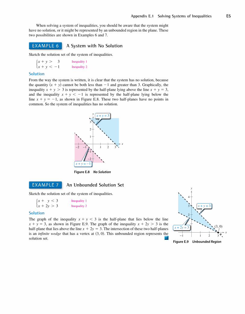
When solving a system of inequalities, you should be aware that the system might have no solution, or it might be represented by an unbounded region in the plane. These two possibilities are shown in Examples 6 and 7.

EXAMPLE 6 A System with No Solution

Sketch the solution set of the system of inequalities.

{x + yx + y

><

3−1

Inequality 1

Inequality 2

SolutionFrom the way the system is written, it is clear that the system has no solution, because the quantity (x + y) cannot be both less than −1 and greater than 3. Graphically, the inequality x + y > 3 is represented by the half-plane lying above the line x + y = 3, and the inequality x + y < −1 is represented by the half-plane lying below the line x + y = −1, as shown in Figure E.8. These two half-planes have no points in common. So the system of inequalities has no solution.

21−1−2 3

1

−2

2

3

y

x

x + y = 3

x + y = −1

−1

Figure E.8 No Solution

EXAMPLE 7 An Unbounded Solution Set

Sketch the solution set of the system of inequalities.

{x +x +

y2y

<>

33

Inequality 1

Inequality 2

SolutionThe graph of the inequality x + y < 3 is the half-plane that lies below the line x + y = 3, as shown in Figure E.9. The graph of the inequality x + 2y > 3 is the half-plane that lies above the line x + 2y = 3. The intersection of these two half-planes is an infinite wedge that has a vertex at (3, 0). This unbounded region represents the solution set.

Figure E.9 Unbounded Region

−1 1 2 3

2

3

4

(3, 0)

x

y

x + y = 3

x + 2y = 3


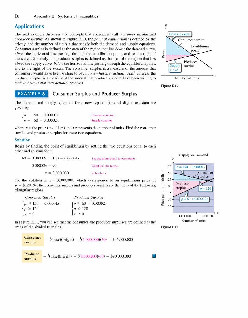
ApplicationsThe next example discusses two concepts that economists call consumer surplus and producer surplus. As shown in Figure E.10, the point of equilibrium is defined by the price p and the number of units x that satisfy both the demand and supply equations. Consumer surplus is defined as the area of the region that lies below the demand curve, above the horizontal line passing through the equilibrium point, and to the right of the p-axis. Similarly, the producer surplus is defined as the area of the region that lies above the supply curve, below the horizontal line passing through the equilibrium point, and to the right of the p-axis. The consumer surplus is a measure of the amount that consumers would have been willing to pay above what they actually paid, whereas the producer surplus is a measure of the amount that producers would have been willing to receive below what they actually received.

EXAMPLE 8 Consumer Surplus and Producer Surplus

The demand and supply equations for a new type of personal digital assistant are given by

{p =p =

150 −60 +

0.00001x0.00002x

Demand equation

Supply equation

where p is the price (in dollars) and x represents the number of units. Find the consumer surplus and producer surplus for these two equations.

SolutionBegin by finding the point of equilibrium by setting the two equations equal to each other and solving for x.

60 + 0.00002x = 150 − 0.00001x Set equations equal to each other.

0.00003x = 90 Combine like terms.

x = 3,000,000 Solve for x.

So, the solution is x = 3,000,000, which corresponds to an equilibrium price of p = $120. So, the consumer surplus and producer surplus are the areas of the following triangular regions.

Consumer Surplus Producer Surplus

{ppx

≤≥≥

150 − 0.00001x1200

{ppx

≥≤≥

60 + 0.00002x1200

In Figure E.11, you can see that the consumer and producer surpluses are defined as the areas of the shaded triangles.

Consumer surplus

= 12(base)(height) = 1

2(3,000,000)(30) = $45,000,000

Producer surplus

= 12(base)(height) = 1

2(3,000,000)(60) = $90,000,000

Figure E.10

Pric

e

Number of units

Producersurplus

Consumer surplus

Equilibriumpoint

p

x

Supplycurve

Demand curve

Figure E.11

Number of units

Pric

e pe

r un

it (i

n do

llars

)

1,000,000 3,000,000

25

50

75

100

125

150

175

Producersurplus

surplus

x

pSupply vs. Demand

Consumer

p = 60 + 0.00002x

p = 120

p = 150 − 0.00001x


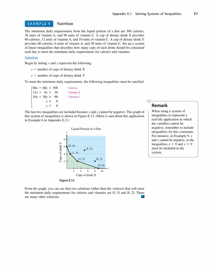
EXAMPLE 9 Nutrition

The minimum daily requirements from the liquid portion of a diet are 300 calories, 36 units of vitamin A, and 90 units of vitamin C. A cup of dietary drink X provides 60 calories, 12 units of vitamin A, and 10 units of vitamin C. A cup of dietary drink Y provides 60 calories, 6 units of vitamin A, and 30 units of vitamin C. Set up a system of linear inequalities that describes how many cups of each drink should be consumed each day to meet the minimum daily requirements for calories and vitamins.

SolutionBegin by letting x and y represent the following.

x = number of cups of dietary drink X

x = number of cups of dietary drink Y

To meet the minimum daily requirements, the following inequalities must be satisfied.

{60x +12x +10x +

60y ≥6y ≥

30y ≥x ≥y ≥

300369000

Calories

Vitamin A

Vitamin C

The last two inequalities are included because x and y cannot be negative. The graph of this system of inequalities is shown in Figure E.12. (More is said about this application in Example 6 in Appendix E.2.)

2 4 6 8 10

2

4

6

8

(3, 2)

(5, 5)

(9, 0)x

y

Cups of drink X

Cup

s of

dri

nk Y

Liquid Portion of a Diet

(0, 6)

(1, 4)

(8, 2)

Figure E.12

From the graph, you can see that two solutions (other than the vertices) that will meet the minimum daily requirements for calories and vitamins are (5, 5) and (8, 2). There are many other solutions.

RemarkWhen using a system of inequalities to represent a real-life application in which the variables cannot be negative, remember to include inequalities for this constraint. For instance, in Example 9, x and y cannot be negative, so the inequalities x ≥ 0 and y ≥ 0 must be included in the system.


E.1 Exercises

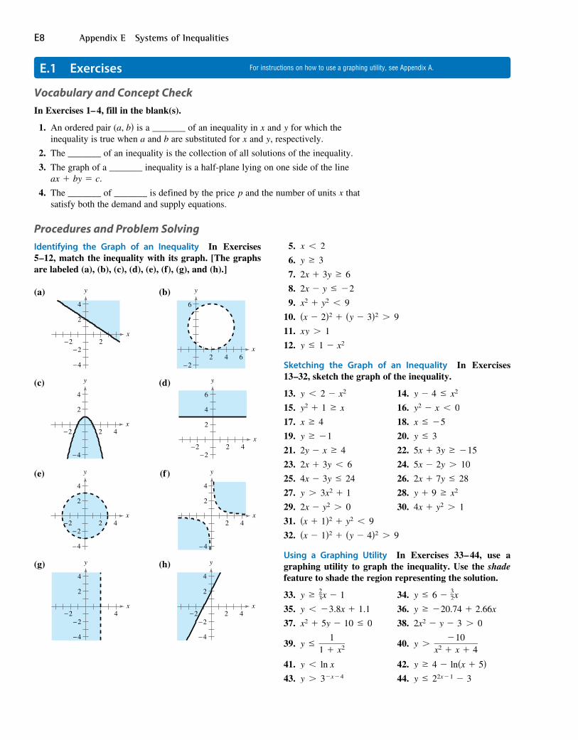
Identifying the Graph of an Inequality In Exercises 5 –12, match the inequality with its graph. [The graphs are labeled (a), (b), (c), (d), (e), (f ), (g), and (h).]

(a)

−2 2−2

−4

2

4

x

y (b)

4 62−2

6

x

y

(c)

−2 42

−4

2

4

x

y (d)

−2 42−2

2

4

6

x

y

(e)

−2 42−2

−4

2

4

x

y (f )

42

−4

2

4

x

y

(g)

−2 4−2

−4

2

4

x

y (h)

−2 42

−4

−2

2

4

x

y

5. x < 2

6. y ≥ 3

7. 2x + 3y ≥ 6

8. 2x − y ≤ −2

9. x2 + y2 < 9

10. (x − 2)2 + (y − 3)2 > 9

11. xy > 1

12. y ≤ 1 − x2

Sketching the Graph of an Inequality In Exercises 13 –32, sketch the graph of the inequality.

13. y < 2 − x2 14. y − 4 ≤ x2

15. y2 + 1 ≥ x 16. y2 − x < 0

17. x ≥ 4 18. x ≤ −5

19. y ≥ −1 20. y ≤ 3

21. 2y − x ≥ 4 22. 5x + 3y ≥ −15

23. 2x + 3y < 6 24. 5x − 2y > 10

25. 4x − 3y ≤ 24 26. 2x + 7y ≤ 28

27. y > 3x2 + 1 28. y + 9 ≥ x2

29. 2x − y2 > 0 30. 4x + y2 > 1

31. (x + 1)2 + y2 < 9

32. (x − 1)2 + (y − 4)2 > 9

Using a Graphing Utility In Exercises 33 – 44, use a graphing utility to graph the inequality. Use the shade feature to shade the region representing the solution.

33. y ≥ 23x − 1 34. y ≤ 6 − 3

2x

35. y < −3.8x + 1.1 36. y ≥ −20.74 + 2.66x

37. x2 + 5y − 10 ≤ 0 38. 2x2 − y − 3 > 0

39. y ≤ 11 + x2 40. y >

−10x2 + x + 4

41. y < ln x 42. y ≥ 4 − ln(x + 5)43. y > 3−x−4 44. y ≤ 22x−1 − 3

Vocabulary and Concept CheckIn Exercises 1– 4, fill in the blank(s).

1. An ordered pair (a, b) is a _______ of an inequality in x and y for which the inequality is true when a and b are substituted for x and y, respectively.

2. The _______ of an inequality is the collection of all solutions of the inequality.

3. The graph of a _______ inequality is a half-plane lying on one side of the line ax + by = c.

4. The _______ of _______ is defined by the price p and the number of units x that satisfy both the demand and supply equations.

Procedures and Problem Solving

For instructions on how to use a graphing utility, see Appendix A.


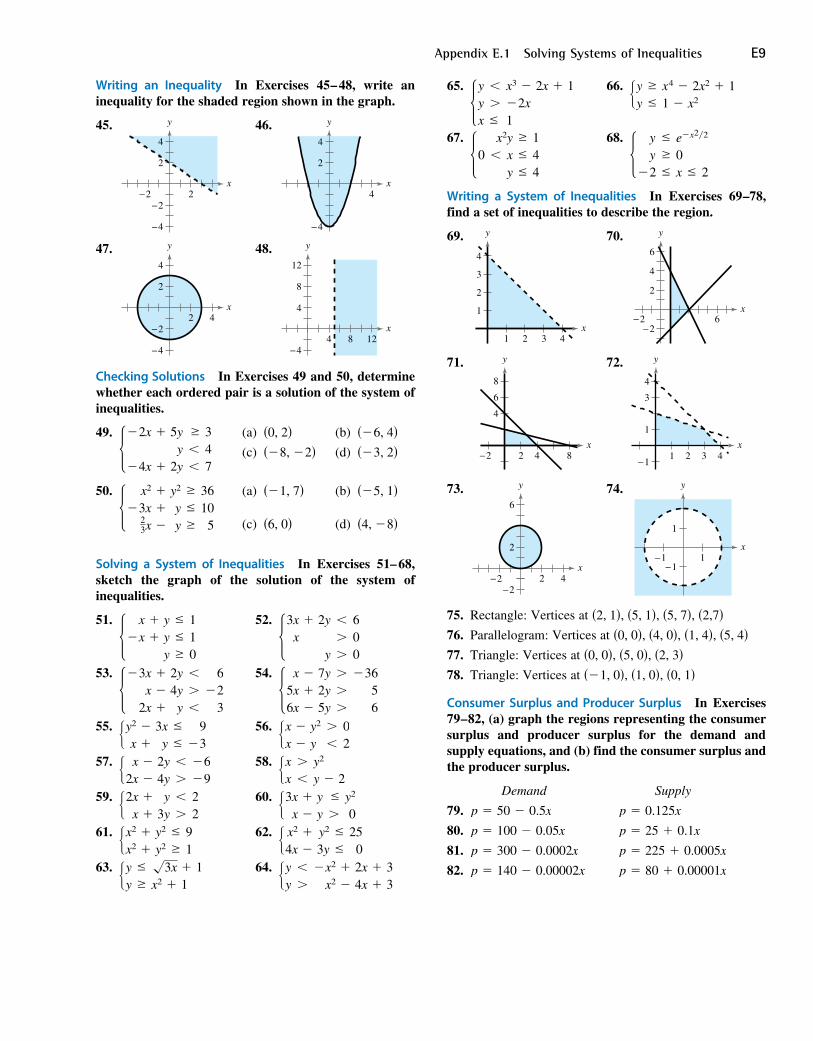
Writing an Inequality In Exercises 45 – 48, write an inequality for the shaded region shown in the graph.

45.

−2 2−2

−4

2

4

x

y 46.

4

−4

2

4

x

y

47.

42−2

−4

2

4

x

y 48.

8 124−4

12

8

4

x

y

Checking Solutions In Exercises 49 and 50, determine whether each ordered pair is a solution of the system of inequalities.

49. {−2x

−4x

+

+

5yy

2y

≥<<

347

(a) (0, 2) (b) (−6, 4) (c) (−8, −2) (d) (−3, 2)

50. { x2

−3x23x

++−

y2

yy

≥≤≥

36105

(a) (−1, 7) (b) (−5, 1)

(c) (6, 0) (d) (4, −8)

Solving a System of Inequalities In Exercises 51– 68, sketch the graph of the solution of the system of inequalities.

51. { x

−x++

yyy

≤≤≥

110

52. {3x

x+ 2y

y

<>>

600

53. {−3x

x2x

+−+

2y4yy

<><

6−2

3

54. { x

5x6x

−+−

7y2y5y

>>>

−3656

55. {y2

x−+

3xy

≤≤

9−3

56.

{xx −−

y2

y><

02

57. { x

2x−−

2y4y

<>

−6−9

58.

{xx ><

y2

y − 259.

{2xx++

y3y

<>

22

60. {3x

x+−

yy

≤>

y2

061.

{x2

x2

++

y2

y2

≤≥

91

62. { x2

4x+−

y2

3y≤≤

250

63. {yy ≤

≥√3x + 1x2 + 1

64. {yy <

>−x2

x2

+ 2x− 4x

+ 3+ 3

65. {yy

x

<>≤

x3 − 2x + 1−2x1

66.

{yy ≥≤

x4 − 2x2 + 11 − x2

67. { x2y

0 < xy

≥≤≤

144

68. {

−

yy2

≤≥≤

e−x2�2

0x ≤ 2

Writing a System of Inequalities In Exercises 69 –78, find a set of inequalities to describe the region.

69.

1 2 3 4

1

2

3

4

y

x

70.

−2 6−2

6

2

4

x

y

71.

2−2 4 8

4

6

8

x

y 72.

1 2−1

1

3

4

x

y

3 4

73.

42−2

−2

2

6

x

y 74.

1−1

1

−1

x

y

75. Rectangle: Vertices at (2, 1), (5, 1), (5, 7), (2,7)76. Parallelogram: Vertices at (0, 0), (4, 0), (1, 4), (5, 4)77. Triangle: Vertices at (0, 0), (5, 0), (2, 3)78. Triangle: Vertices at (−1, 0), (1, 0), (0, 1)

Consumer Surplus and Producer Surplus In Exercises 79 – 82, (a) graph the regions representing the consumer surplus and producer surplus for the demand and supply equations, and (b) find the consumer surplus and the producer surplus.

Demand Supply

79. p = 50 − 0.5x p = 0.125x

80. p = 100 − 0.05x p = 25 + 0.1x

81. p = 300 − 0.0002x p = 225 + 0.0005x

82. p = 140 − 0.00002x p = 80 + 0.00001x


Solving a System of Inequalities In Exercises 83 – 86, (a) find a system of inequalities that models the problem and (b) graph the system, shading the region that represents the solution of the system.

83. Finance A person plans to invest some or all of $30,000 in two different interest-bearing accounts. Each account is to contain at least $7500, and one account should have at least twice the amount that is in the other account.

84. Arts Management For a summer concert event, one type of ticket costs $20 and another costs $35. The promoter of the concert must sell at least 20,000 tickets, including at least 10,000 of the $20 tickets and at least 5000 of the $35 tickets, and the gross receipts must total at least $300,000 in order for the concert to be held.

85. (p. E1) A dietitian is asked to design a special dietary supplement using two different foods. The minimum daily requirements of the new supplement are 280 units of calcium, 160 units of iron, and 180 units of vitamin B. Each ounce of food X contains 20 units of calcium, 15 units of iron, and 10 units of vitamin B. Each ounce of food Y contains 10 units of calcium, 10 units of iron, and 20 units of vitamin B.

86. Retail Management A store sells two models of computers. Because of the demand, the store stocks at least twice as many units of model A as units of model B. The costs to the store for models A and B are $800 and $1200, respectively. The management does not want more than $20,000 in computer inventory at any one time, and it wants at least four model A computers and two model B computers in inventory at all times.

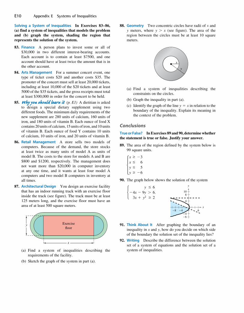
87. Architectural Design You design an exercise facility that has an indoor running track with an exercise floor inside the track (see figure). The track must be at least 125 meters long, and the exercise floor must have an area of at least 500 square meters.

Exercise�oor

x

y

(a) Find a system of inequalities describing the requirements of the facility.

(b) Sketch the graph of the system in part (a).

88. Geometry Two concentric circles have radii of x and y meters, where y > x (see figure). The area of the region between the circles must be at least 10 square meters.

x

y

(a) Find a system of inequalities describing the constraints on the circles.

(b) Graph the inequality in part (a).

(c) Identify the graph of the line y = x in relation to the boundary of the inequality. Explain its meaning in the context of the problem.

ConclusionsTrue or False? In Exercises 89 and 90, determine whether the statement is true or false. Justify your answer.

89. The area of the region defined by the system below is 99 square units.

{xxyy

≥≤≤≥

−365

−6

90. The graph below shows the solution of the system

{−4x3x

−+

y9yy2

≤>≥

662.

6−4−4

4

810

−6

−8x

y

91. Think About It After graphing the boundary of an inequality in x and y, how do you decide on which side of the boundary the solution set of the inequality lies?

92. Writing Describe the difference between the solution set of a system of equations and the solution set of a system of inequalities.

Appendix E.2 Linear Programming E11

Linear Programming: A Graphical ApproachMany applications in business and economics involve a process called optimization, in which you are asked to find the minimum or maximum value of a quantity. In this appendix, you will study an optimization strategy called linear programming.

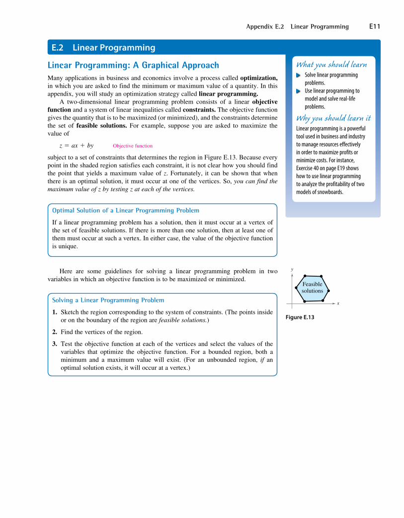
A two-dimensional linear programming problem consists of a linear objective function and a system of linear inequalities called constraints. The objective function gives the quantity that is to be maximized (or minimized), and the constraints determine the set of feasible solutions. For example, suppose you are asked to maximize the value of

z = ax + by Objective function

subject to a set of constraints that determines the region in Figure E.13. Because every point in the shaded region satisfies each constraint, it is not clear how you should find the point that yields a maximum value of z. Fortunately, it can be shown that when there is an optimal solution, it must occur at one of the vertices. So, you can find the maximum value of z by testing z at each of the vertices.

Optimal Solution of a Linear Programming Problem

If a linear programming problem has a solution, then it must occur at a vertex of the set of feasible solutions. If there is more than one solution, then at least one of them must occur at such a vertex. In either case, the value of the objective function is unique.

Here are some guidelines for solving a linear programming problem in two variables in which an objective function is to be maximized or minimized.

Solving a Linear Programming Problem

1. Sketch the region corresponding to the system of constraints. (The points inside or on the boundary of the region are feasible solutions.)

2. Find the vertices of the region.

3. Test the objective function at each of the vertices and select the values of the variables that optimize the objective function. For a bounded region, both a minimum and a maximum value will exist. (For an unbounded region, if an optimal solution exists, it will occur at a vertex.)

E.2 Linear Programming

What you should learn Solve linear programming

problems. Use linear programming to

model and solve real-life problems.

Why you should learn itLinear programming is a powerful tool used in business and industry to manage resources effectively in order to maximize profits or minimize costs. For instance, Exercise 40 on page E19 shows how to use linear programming to analyze the profitability of two models of snowboards.

Figure E.13

x

Feasiblesolutions

y


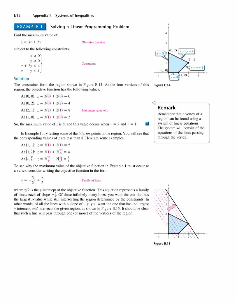
EXAMPLE 1 Solving a Linear Programming Problem

Find the maximum value of

z = 3x + 2y Objective function

subject to the following constraints.

x +x −

xy

2yy

≥≥≤≤

0041} Constraints

SolutionThe constraints form the region shown in Figure E.14. At the four vertices of this region, the objective function has the following values.

At (0, 0): z = 3(0) + 2(0) = 0

At (0, 2): z = 3(0) + 2(2) = 4

At (2, 1): z = 3(2) + 2(1) = 8 Maximum value of z

At (1, 0): z = 3(1) + 2(0) = 3

So, the maximum value of z is 8, and this value occurs when x = 2 and y = 1.

In Example 1, try testing some of the interior points in the region. You will see that the corresponding values of z are less than 8. Here are some examples.

At (1, 1): z = 3(1) + 2(1) = 5

At (1, 12): z = 3(1) + 2(12) = 4

At (12, 32): z = 3(1

2) + 2(32) = 9

2

To see why the maximum value of the objective function in Example 1 must occur at a vertex, consider writing the objective function in the form

y = −32

x +z2

Family of lines

where z�2 is the y-intercept of the objective function. This equation represents a family of lines, each of slope −3

2. Of these infinitely many lines, you want the one that has the largest z-value while still intersecting the region determined by the constraints. In other words, of all the lines with a slope of −3

2, you want the one that has the largest y-intercept and intersects the given region, as shown in Figure E.15. It should be clear that such a line will pass through one (or more) of the vertices of the region.

RemarkRemember that a vertex of a region can be found using a system of linear equations. The system will consist of the equations of the lines passing through the vertex.

Figure E.14

x = 0x + 2y = 4

x(0, 0)

(0, 2)

(2, 1)

(1, 0)

y

−1 2 3

1

2

3

4

y = 0

x − y = 1

Figure E.15

x

y

−1 1 2

1

2

3

4


The next example shows that the same basic procedure can be used to solve a problem in which the objective function is to be minimized.


Find the minimum value of


where x ≥ 0 and y ≥ 0, subject to the following constraints.

2x +3x −−x +2x +

3yyy

5y

≥≤≤≤

6154

27} Constraints

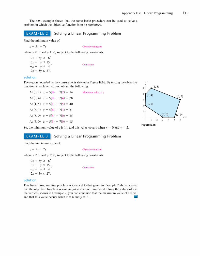
SolutionThe region bounded by the constraints is shown in Figure E.16. By testing the objective function at each vertex, you obtain the following.

At (0, 2): z = 5(0) + 7(2) = 14 Minimum value of z

At (0, 4): z = 5(0) + 7(4) = 28

At (1, 5): z = 5(1) + 7(5) = 40

At (6, 3): z = 5(6) + 7(3) = 51

At (5, 0): z = 5(5) + 7(0) = 25

At (3, 0): z = 5(3) + 7(0) = 15

So, the minimum value of z is 14, and this value occurs when x = 0 and y = 2.





2x +3x −−x +2x +

3yyy

5y

≥≤≤≤

6154

27} Constraints

SolutionThis linear programming problem is identical to that given in Example 2 above, except that the objective function is maximized instead of minimized. Using the values of z at the vertices shown in Example 2, you can conclude that the maximum value of z is 51, and that this value occurs when x = 6 and y = 3.

Figure E.16

1 2 3 4 5 6

1

2

3

4

5

(0, 2)

(0, 4)

(1, 5)

(6, 3)

(3, 0) (5, 0)

y

x


It is possible for the maximum (or minimum) value in a linear programming problem to occur at two different vertices. For instance, at the vertices of the region shown in Figure E.17, the objective function


has the following values.

At (0, 0): z = 2(0) + 2(0) = 0

At (0, 4): z = 2(0) + 2(4) = 8



At (5, 0): z = 2(5) + 2(0) = 10

In this case, you can conclude that the objective function has a maximum value (of 12) not only at the vertices (2, 4) and (5, 1), but also at any point on the line segment connecting these two vertices, as shown in Figure E.17. Note that by rewriting the objective function as

y = −x +12

z

you can see that its graph has the same slope as the line through the vertices (2, 4) and (5, 1).

Some linear programming problems have no optimal solutions. This can occur when the region determined by the constraints is unbounded.

EXAMPLE 4 An Unbounded Region




x +3x +−x +

2y ≥y ≥

2y ≤

477} Constraints

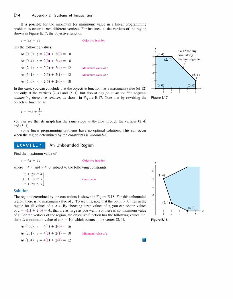
SolutionThe region determined by the constraints is shown in Figure E.18. For this unbounded region, there is no maximum value of z. To see this, note that the point (x, 0) lies in the region for all values of x ≥ 4. By choosing large values of x, you can obtain values of z = 4(x) + 2(0) = 4x that are as large as you want. So, there is no maximum value of z. For the vertices of the region, the objective function has the following values. So, there is a minimum value of z, z = 10, which occurs at the vertex (2, 1).

At (4, 0): z = 4(4) + 2(0) = 16

At (2, 1): z = 4(2) + 2(1) = 10 Minimum value of z

At (1, 4): z = 4(1) + 2(4) = 12

Figure E.17

1 2 3 4 5

1

2

3

4(0, 4)

(2, 4)

(0, 0) (5, 0)

(5, 1)

z = 12 for anypoint alongthis line segment.

y

x

Figure E.18

1 2 3 4 5

1

2

3

4

5

(1, 4)

(2, 1)

(4, 0)

y

x


ApplicationsExample 5 shows how linear programming can be used to find the maximum profit in a business application.

EXAMPLE 5 Optimizing Profit

A manufacturer wants to maximize the profit from selling two types of boxed chocolates. A box of chocolate covered creams yields a profit of $1.50, and a box of chocolate covered cherries yields a profit of $2.00. Market tests and available resources have indicated the following constraints.

1. The combined production level should not exceed 1200 boxes per month.

2. The demand for a box of chocolate covered cherries is no more than half the demand for a box of chocolate covered creams.

3. The production level of a box of chocolate covered creams is less than or equal to 600 boxes plus three times the production level of a box of chocolate covered cherries.

What is the maximum monthly profit? How many boxes of each type should be produced per month to yield the maximum monthly profit?

SolutionLet x be the number of boxes of chocolate covered creams and y be the number of boxes of chocolate covered cherries. The objective function (for the combined profit) is given by

P = 1.5x + 2y. Objective function

The three constraints translate into the following linear inequalities.

1. x + y ≤ 1200 x + y ≤ 1200

2. y ≤ 12x −x + 2y ≤ 0

3. x ≤ 3y + 600 x − 3y ≤ 600

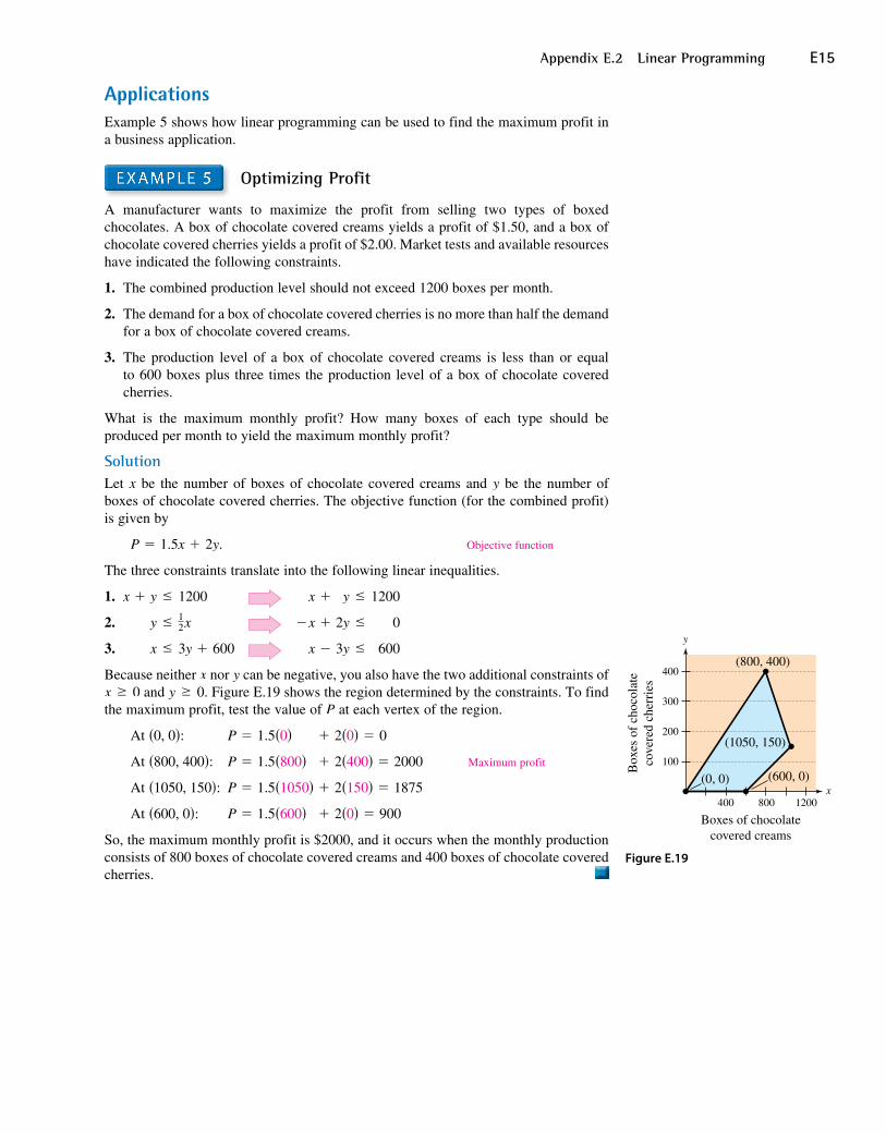
Because neither x nor y can be negative, you also have the two additional constraints of x ≥ 0 and y ≥ 0. Figure E.19 shows the region determined by the constraints. To find the maximum profit, test the value of P at each vertex of the region.

At (0, 0): P = 1.5(0) + 2(0) = 0

At (800, 400): P = 1.5(800) + 2(400) = 2000 Maximum profit

At (1050, 150): P = 1.5(1050) + 2(150) = 1875

At (600, 0): P = 1.5(600) + 2(0) = 900

So, the maximum monthly profit is $2000, and it occurs when the monthly production consists of 800 boxes of chocolate covered creams and 400 boxes of chocolate covered cherries.

Figure E.19

Boxes of chocolatecovered creams

Box

es o

f ch

ocol

ate

cove

red

cher

ries

1200800400

100

200

300

400(800, 400)

(1050, 150)

(600, 0)(0, 0)

y

x


In Example 5, suppose the manufacturer improves the production of chocolate covered creams so that a profit of $2.50 per box is obtained. The maximum profit can now be found using the objective function P = 2.5x + 2y. By testing the values of P at the vertices of the region, you find that the maximum profit is now $2925, which occurs when x = 1050 and y = 150.

EXAMPLE 6 Optimizing Cost

The minimum daily requirements from the liquid portion of a diet are 300 calories, 36 units of vitamin A, and 90 units of vitamin C. A cup of dietary drink X costs $0.12 and provides 60 calories, 12 units of vitamin A, and 10 units of vitamin C. A cup of dietary drink Y costs $0.15 and provides 60 calories, 6 units of vitamin A, and 30 units of vitamin C. How many cups of each drink should be consumed each day to minimize the cost and still meet the daily requirements?

SolutionAs in Example 9 on page E7, let x be the number of cups of dietary drink X and let y be the number of cups of dietary drink Y.

For Calories:For Vitamin A:For Vitamin C:

60x +12x +10x +

60y ≥6y ≥

30y ≥x ≥y ≥

300369000

} Constraints

The cost C is given by

C = 0.12x + 0.15y. Objective function

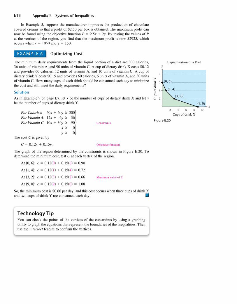
The graph of the region determined by the constraints is shown in Figure E.20. To determine the minimum cost, test C at each vertex of the region.

At (0, 6): c = 0.12(0) + 0.15(6) = 0.90

At (1, 4): c = 0.12(1) + 0.15(4) = 0.72

At (3, 2): c = 0.12(3) + 0.15(2) = 0.66 Minimum value of C

At (9, 0): c = 0.12(9) + 0.15(0) = 1.08

So, the minimum cost is $0.66 per day, and this cost occurs when three cups of drink X and two cups of drink Y are consumed each day.

Technology TipYou can check the points of the vertices of the constraints by using a graphing utility to graph the equations that represent the boundaries of the inequalities. Then use the intersect feature to confirm the vertices.

Figure E.20

2 4 6 8 10

2

4

6

8

(3, 2)

(9, 0)x

y

Cups of drink X

Cup

s of

dri

nk Y

Liquid Portion of a Diet

(0, 6)

(1, 4)


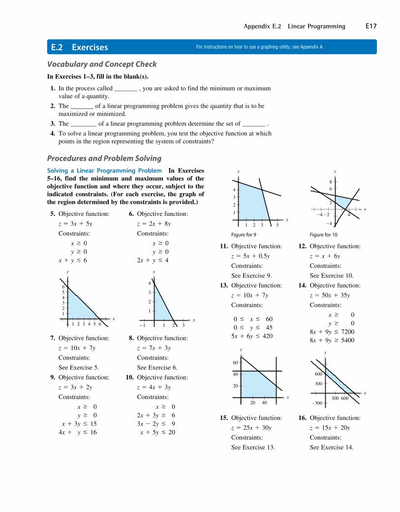
Solving a Linear Programming Problem In Exercises 5–16, find the minimum and maximum values of the objective function and where they occur, subject to the indicated constraints. (For each exercise, the graph of the region determined by the constraints is provided.)

5. Objective function: 6. Objective function:

z = 3x + 5y z = 2x + 8y

Constraints: Constraints:

x +

x ≥y ≥y ≤

006

2x +

x ≥y ≥y ≤

004

1 2 3 4 5 6

123456

x

y

−1 1 2 3

2

1

3

4

y

x


z = 10x + 7y z = 7x + 3y


See Exercise 5. See Exercise 6.


z = 3x + 2y z = 4x + 3y


x +

4x +

x ≥y ≥

3y ≤y ≤

00

1516

2x +3x −x +

x ≥3y ≥2y ≤5y ≤

069

20

1 532

2

1

3

4

y

x

−2−4 4

−4

2

6

8

x

y

Figure for 9 Figure for 10


z = 5x + 0.5y z = x + 6y




z = 10x + 7y z = 50x + 35y


0 ≤0 ≤

5x +

x ≤y ≤

6y ≤

6045

420

8x +8x +

x ≥y ≥

9y ≤9y ≥

00

72005400

20 40

20

40

60

x

y

300 600−300

300

600

y

x


z = 25x + 30y z = 15x + 20y



Vocabulary and Concept CheckIn Exercises 1– 3, fill in the blank(s).

1. In the process called _______ , you are asked to find the minimum or maximum value of a quantity.

2. The _______ of a linear programming problem gives the quantity that is to be maximized or minimized.

3. The ________ of a linear programming problem determine the set of _______ .

4. To solve a linear programming problem, you test the objective function at which points in the region representing the system of constraints?

Procedures and Problem Solving

E.2 Exercises For instructions on how to use a graphing utility, see Appendix A.


Solving a Linear Programming Problem In Exercises 17– 30, sketch the region determined by the constraints. Then find the minimum and maximum values of the objective function and where they occur, subject to the indicated constraints.


z = 6x + 10y z = 7x + 8y


2x +

x ≥y ≥

5y ≤

00

10

x +

x ≥y ≥

12y ≤

004


z = 3x + 4y z = 4x + 5y


2x +4x +

x ≥y ≥

5y ≤y ≤

00

5028

2x +x +

x ≥y ≥

2y ≤2y ≤

00

106


z = x + 2y z = 2x + 4y




z = 2x z = 3y




z = 4x + y z = x


x +

2x +

x ≥y ≥

2y ≤3y ≥

00

4072

2x +2x +4x +

x ≥y ≥

3y ≤y ≤y ≤

00

602848


z = x + 4y z = y




z = 2x + 3y z = 3x + 2y



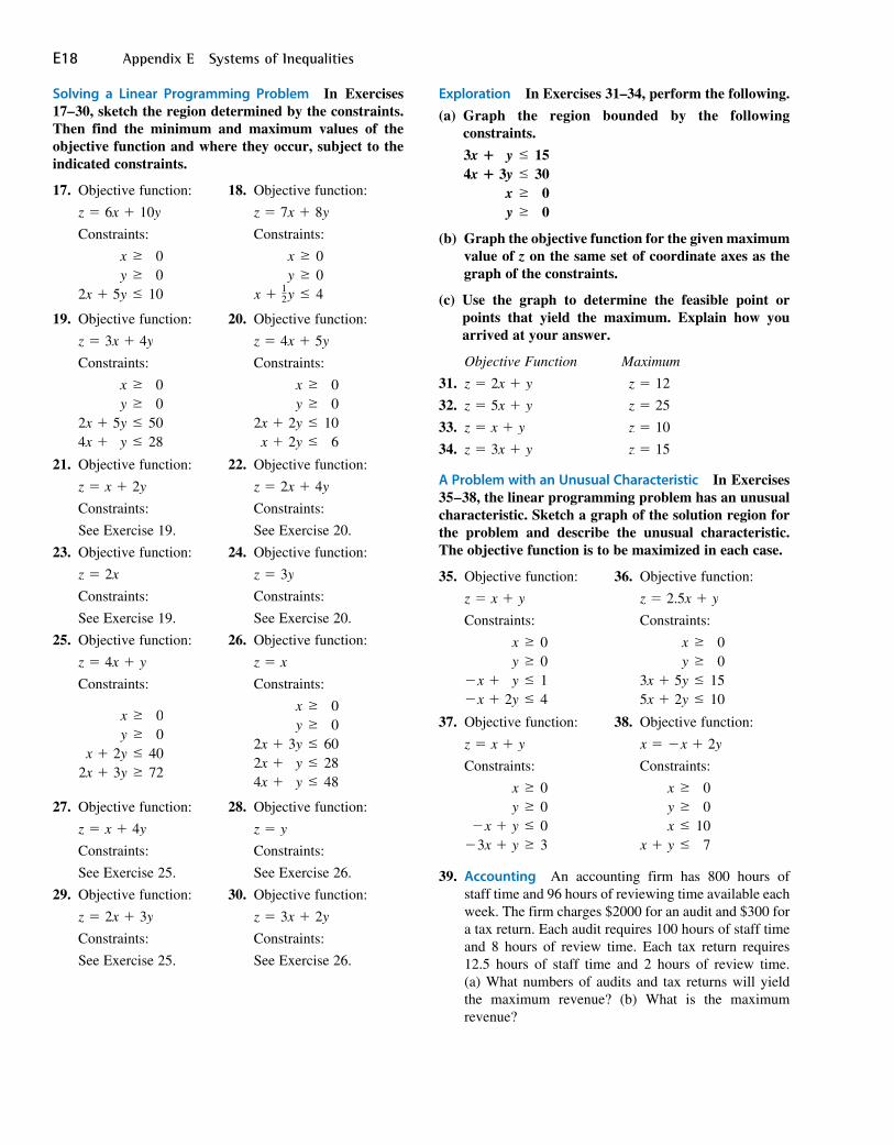
Exploration In Exercises 31–34, perform the following.

(a) Graph the region bounded by the following constraints.

3x +4x +

y ≤3y ≤x ≥y ≥

153000

(b) Graph the objective function for the given maximum value of z on the same set of coordinate axes as the graph of the constraints.

(c) Use the graph to determine the feasible point or points that yield the maximum. Explain how you arrived at your answer.

Objective Function Maximum

31. z = 2x + y z = 12

32. z = 5x + y z = 25

33. z = x + y z = 10

34. z = 3x + y z = 15

A Problem with an Unusual Characteristic In Exercises 35 – 38, the linear programming problem has an unusual characteristic. Sketch a graph of the solution region for the problem and describe the unusual characteristic. The objective function is to be maximized in each case.


z = x + y z = 2.5x + y


−x +−x +

x ≥y ≥y ≤

2y ≤

0014

3x +5x +

x ≥y ≥

5y ≤2y ≤

00

1510


z = x + y x = −x + 2y


−x +−3x +

x ≥y ≥y ≤y ≥

0003

x +

x ≥y ≥x ≤y ≤

00

107

39. Accounting An accounting firm has 800 hours of staff time and 96 hours of reviewing time available each week. The firm charges $2000 for an audit and $300 for a tax return. Each audit requires 100 hours of staff time and 8 hours of review time. Each tax return requires 12.5 hours of staff time and 2 hours of review time. (a) What numbers of audits and tax returns will yield the maximum revenue? (b) What is the maximum revenue?


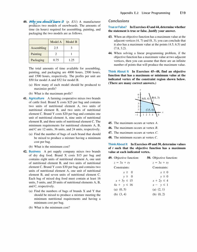
40. (p. E11) A manufacturer produces two models of snowboards. The amounts of time (in hours) required for assembling, painting, and packaging the two models are as follows.

Model A Model B

Assembling 2.5 3

Painting 2 1

Packaging 0.75 1.25

The total amounts of time available for assembling, painting, and packaging are 4000 hours, 2500 hours, and 1500 hours, respectively. The profits per unit are $50 for model A and $52 for model B.

(a) How many of each model should be produced to maximize profit?

(b) What is the maximum profit?

41. Agriculture A farming cooperative mixes two brands of cattle feed. Brand X costs $25 per bag and contains two units of nutritional element A, two units of nutritional element B, and two units of nutritional element C. Brand Y costs $20 per bag and contains one unit of nutritional element A, nine units of nutritional element B, and three units of nutritional element C. The minimum requirements for nutritional elements A, B, and C are 12 units, 36 units, and 24 units, respectively.

(a) Find the number of bags of each brand that should be mixed to produce a mixture having a minimum cost per bag.

(b) What is the minimum cost?

42. Business A pet supply company mixes two brands of dry dog food. Brand X costs $15 per bag and contains eight units of nutritional element A, one unit of nutritional element B, and two units of nutritional element C. Brand Y costs $30 per bag and contains two units of nutritional element A, one unit of nutritional element B, and seven units of nutritional element C. Each bag of mixed dog food must contain at least 16 units, 5 units, and 20 units of nutritional elements A, B, and C, respectively.

(a) Find the numbers of bags of brands X and Y that should be mixed to produce a mixture meeting the minimum nutritional requirements and having a minimum cost per bag.

(b) What is the minimum cost?

ConclusionsTrue or False? In Exercises 43 and 44, determine whether the statement is true or false. Justify your answer.

43. When an objective function has a maximum value at the adjacent vertices (4, 7) and (8, 3), you can conclude that it also has a maximum value at the points (4.5, 6.5) and (7.8, 3.2).

44. When solving a linear programming problem, if the objective function has a maximum value at two adjacent vertices, then you can assume that there are an infinite number of points that will produce the maximum value.

Think About It In Exercises 45 – 48, find an objective function that has a maximum or minimum value at the indicated vertex of the constraint region shown below. (There are many correct answers.)

−1 1 6432

123

56

B(4, 3)A(0, 4)

C(5, 0)x

y

45. The maximum occurs at vertex A.

46. The maximum occurs at vertex B.

47. The maximum occurs at vertex C.

48. The minimum occurs at vertex C.

Think About It In Exercises 49 and 50, determine values of t such that the objective function has a maximum value at each indicated vertex.


z = 3x + ty z = 3x + ty


x +

4x +

x ≥y ≥

3y ≤y ≤

00

1516

x +x −

x ≥y ≥

2y ≤y ≤

0041

(a) (0, 5) (a) (2, 1) (b) (3, 4) (b) (0, 2)

Documents

Appendix E: Systems of Inequalities - Cengage · E1 The Graph of an Inequality The statements 3x − 2y < 6 and 2x2 + 3y2 ≥ 6 are inequalities in two variables. An ordered pair