Embed Size (px)
Citation preview

APPENDIX E: REGIONAL PEST
MANAGEMENT STRATEGY
COST BENEFIT ANALYSIS –
TENAX CONSULTING LIMITED
FOR THE BAY OF PLENTY
REGIONAL COUNCIL

Pest impact assessment and cost-benefit analysis for the
proposed Bay of Plenty Regional Pest Management Strategy
Jon J. Sullivan1, Melissa Hutchison2
1 Bio-Protection Research CentrePO Box 84, Lincoln University
Lincoln 7647, New [email protected]
2 Tenax Consulting Ltd16 Samuel Street, Christchurch
May 2010

©2010, (version 31 May 2010) Bio-Protection Research Centre, Lincoln University.Report prepared by the Bio-Protection Research Centre for Environment Bay of Plenty, May 2010. Anypublication, reproduction, or adaptation of this report must be authorised by Environment Bay of Plenty.

Executive Summary
This report assesses the impacts of plant and animal pests listed in the proposed Bay ofPlenty Regional Pest Management Strategy (RPMS) and evaluates the costs and benefitsof the proposed regional actions. This is done to meet the requirements of Section 72(1)of the New Zealand Biosecurity Act 1993.
We use data from Environment Bay of Plenty sta↵ and published information to summarisethe known impacts of 44 pest plants and 23 pest animals on production values as well asnatural, social, and cultural values.
We perform cost-benefit analyses (CBAs) on each species using a modified version ofthe Harris Model. The Harris Model was developed in 2000 by economist Simon Harrisspecifically for RPMS assessments and it has been commonly used. Our modificationsto the Harris Model are designed to make it both more diverse and less precise in itsdata requirements. These make it more capable of incorporating the diverse range ofpests and impacts that face the Bay of Plenty region, while retaining its robust economicfoundations.
In addition to our standard assessments of impacts, costs, and benefits for the many pests,we also provide more detailed assessments for pests of special concern. The pests of specialinterest to the Environment Bay of Plenty regional council were wilding pines, gorse inlake catchments where it contributes to nitrogen leaching into lakes, pest fish (gambusiaand the coarse fish brown catfish, koi carp, perch, rudd, and tench), and boundary controlof the three widespread weeds, gorse, blackberry, and ragwort.

Contents
1 Introduction 11.1 Introduction . . . . . . . . . . . . . . . . . . . . . . . . . . . . . . . . . . . . 11.2 Methodology . . . . . . . . . . . . . . . . . . . . . . . . . . . . . . . . . . . 11.3 Assumptions . . . . . . . . . . . . . . . . . . . . . . . . . . . . . . . . . . . 31.4 Determining beneficiaries and exacerbators . . . . . . . . . . . . . . . . . . 3
2 Pest plants (weeds) 52.1 Pest plants . . . . . . . . . . . . . . . . . . . . . . . . . . . . . . . . . . . . 5
2.1.1 African feather grass (Pennisetum macrourum) . . . . . . . . . . . . 92.1.2 Alligator weed (Alternanthera philoxeroides) . . . . . . . . . . . . . 142.1.3 Apple of Sodom (Solanum linnaeanum) . . . . . . . . . . . . . . . . 192.1.4 Asiatic knotweed (Reynoutria japonica) . . . . . . . . . . . . . . . . 242.1.5 Banana passionfruit (Passiflora tripartita var.mollissima, P. tarmini-
ana, P. caerulea) . . . . . . . . . . . . . . . . . . . . . . . . . . . . . 292.1.6 Blackberry (Rubus fruticosus agg.) . . . . . . . . . . . . . . . . . . . 342.1.7 Boneseed (Chrysanthemoides monilifera) . . . . . . . . . . . . . . . 392.1.8 Cathedral bells (Cobaea scandens) . . . . . . . . . . . . . . . . . . . 442.1.9 Chilean rhubarb (Gunnera tinctoria) . . . . . . . . . . . . . . . . . . 492.1.10 Climbing spindleberry (Celastrus orbiculatus) . . . . . . . . . . . . . 542.1.11 Coast tea tree (Leptospermum laevigatum) . . . . . . . . . . . . . . 592.1.12 Darwin’s barberry (Berberis darwinii) . . . . . . . . . . . . . . . . . 642.1.13 Egeria densa (Egeria densa) . . . . . . . . . . . . . . . . . . . . . . . 692.1.14 Elodea canadensis (Elodea canadensis) . . . . . . . . . . . . . . . . . 712.1.15 Gorse (Ulex europaeus) . . . . . . . . . . . . . . . . . . . . . . . . . 772.1.16 Green goddess lily (Zantedeschia aethiopica “Green goddess”) . . . . 822.1.17 Hornwort (Ceratophyllum demersum) . . . . . . . . . . . . . . . . . 872.1.18 Horse nettle (Solanum carolinense) . . . . . . . . . . . . . . . . . . . 912.1.19 Italian buckthorn (Rhamnus alaternus) . . . . . . . . . . . . . . . . 962.1.20 Kudzu vine (Pueraria montana var.lobata) . . . . . . . . . . . . . . 1012.1.21 Lagarosiphon (Lagarosiphon major) . . . . . . . . . . . . . . . . . . 1062.1.22 Lantana (Lantana camara var.aculeata) . . . . . . . . . . . . . . . . 1102.1.23 Marshwort (Nymphoides geminata) . . . . . . . . . . . . . . . . . . . 1152.1.24 Nassella tussock (Nassella trichotoma) . . . . . . . . . . . . . . . . . 1172.1.25 Noogoora bur (Xanthium strumarium) . . . . . . . . . . . . . . . . . 1222.1.26 Old man’s beard (Clematis vitalba) . . . . . . . . . . . . . . . . . . . 1272.1.27 Pampas (Cortaderia selloana, C. jubata and cultivars) . . . . . . . . 1322.1.28 Privet (Ligustrum lucidum, L. sinense) . . . . . . . . . . . . . . . . 1372.1.29 Ragwort (Senecio jacobaea) . . . . . . . . . . . . . . . . . . . . . . . 142

2.1.30 Royal fern (Osmunda regalis) . . . . . . . . . . . . . . . . . . . . . . 1472.1.31 Saltwater paspalum (Paspalum vaginatum) . . . . . . . . . . . . . . 1522.1.32 Senegal tea (Gymnocoronis spilanthoides) . . . . . . . . . . . . . . . 1572.1.33 Spartina (Spartina anglica, S. alterniflora, S. . . . . . . . . . . . . . 1592.1.34 Strawberry dogwood (Dendrobenthamia capitata) . . . . . . . . . . . 1642.1.35 Variegated thistle (Silybum marianum) . . . . . . . . . . . . . . . . 1692.1.36 Water poppy (Hydrocleys nymphoides) . . . . . . . . . . . . . . . . . 1742.1.37 White-edged nightshade (Solanum marginatum) . . . . . . . . . . . 1762.1.38 Wild ginger (yellow and kahili) (Hedychium gardnerianum, H. flavescens)1812.1.39 Wild kiwifruit (Actinidia spp.) . . . . . . . . . . . . . . . . . . . . . 1862.1.40 Wild purple loosestrife (Lythrum salicaria) . . . . . . . . . . . . . . 1912.1.41 Woolly nightshade (Solanum mauritianum) . . . . . . . . . . . . . . 1932.1.42 Yellow flag iris (Iris pseudacorus) . . . . . . . . . . . . . . . . . . . . 1982.1.43 Pest plant beneficiaries and exacerbators . . . . . . . . . . . . . . . . 203
3 Pest animals 2063.1 Pest animals . . . . . . . . . . . . . . . . . . . . . . . . . . . . . . . . . . . 206
3.1.1 Argentine ant (Linepithema humile) . . . . . . . . . . . . . . . . . . 2083.1.2 Darwin ant (Doleromyrma darwiniana) . . . . . . . . . . . . . . . . 2133.1.3 Eastern rosella (Platycerus eximius) . . . . . . . . . . . . . . . . . . 2183.1.4 Feral cat (Felis catus) . . . . . . . . . . . . . . . . . . . . . . . . . . 2233.1.5 Feral goat (Capra hircus) . . . . . . . . . . . . . . . . . . . . . . . . 2283.1.6 Ferret (Mustela furo) . . . . . . . . . . . . . . . . . . . . . . . . . . . 2333.1.7 Hedgehog (Erinaceus europaeus) . . . . . . . . . . . . . . . . . . . . 2383.1.8 Magpie (Gymnorhina hypoleuca) . . . . . . . . . . . . . . . . . . . . 2433.1.9 Mouse (Mus musculus) . . . . . . . . . . . . . . . . . . . . . . . . . 2483.1.10 Possum (Trichosurus vulpecula) . . . . . . . . . . . . . . . . . . . . . 2533.1.11 Rabbit (Oryctolagus cuniculus) . . . . . . . . . . . . . . . . . . . . . 2593.1.12 Rat (ship and Norway) (Rattus rattus, R. norvegicus) . . . . . . . . 2643.1.13 Rook (Corvus frugilegus) . . . . . . . . . . . . . . . . . . . . . . . . 2693.1.14 Stoat (Mustela ermina) . . . . . . . . . . . . . . . . . . . . . . . . . 2743.1.15 Wallaby (Macropus eugenii) . . . . . . . . . . . . . . . . . . . . . . . 2793.1.16 Wasp (Vespula spp., Polistes spp.) . . . . . . . . . . . . . . . . . . . 2833.1.17 Weasel (Mustela nivalis) . . . . . . . . . . . . . . . . . . . . . . . . . 2883.1.18 Pest animal beneficiaries and exacerbators . . . . . . . . . . . . . . . 293
4 Pests of special concern 2964.1 Wilding pines . . . . . . . . . . . . . . . . . . . . . . . . . . . . . . . . . . . 296
4.1.1 Introduction . . . . . . . . . . . . . . . . . . . . . . . . . . . . . . . 2964.1.2 Wilding pine species . . . . . . . . . . . . . . . . . . . . . . . . . . . 2974.1.3 Carbon costs of tree weed control . . . . . . . . . . . . . . . . . . . . 2984.1.4 Wilding pine impacts and CBA . . . . . . . . . . . . . . . . . . . . . 2984.1.5 Lodgepole pine (Pinus contorta) . . . . . . . . . . . . . . . . . . . . 3014.1.6 Wilding pine conclusions & recommendations . . . . . . . . . . . . . 309
4.2 Lake gorse . . . . . . . . . . . . . . . . . . . . . . . . . . . . . . . . . . . . . 3114.2.1 Introduction . . . . . . . . . . . . . . . . . . . . . . . . . . . . . . . 3114.2.2 Gorse, a brief natural history . . . . . . . . . . . . . . . . . . . . . . 3124.2.3 Lake gorse impacts and CBA . . . . . . . . . . . . . . . . . . . . . . 3124.2.4 Lake gorse conclusions & recommendations . . . . . . . . . . . . . . 319
4.3 Pest fish . . . . . . . . . . . . . . . . . . . . . . . . . . . . . . . . . . . . . . 321

4.3.1 Introduction . . . . . . . . . . . . . . . . . . . . . . . . . . . . . . . 3214.3.2 Species . . . . . . . . . . . . . . . . . . . . . . . . . . . . . . . . . . 3214.3.3 Pest fish Impacts and CBA . . . . . . . . . . . . . . . . . . . . . . . 3224.3.4 Brown bullhead catfish, Ameiurus nebulosus . . . . . . . . . . . . . 3234.3.5 Catfish (Ameiurus nebulosus) . . . . . . . . . . . . . . . . . . . . . . 3234.3.6 Koi carp, Cyprinus carpio . . . . . . . . . . . . . . . . . . . . . . . . 3264.3.7 Koi carp (Cyprinus carpio) . . . . . . . . . . . . . . . . . . . . . . . 3274.3.8 Perch, Perca fluviatilis . . . . . . . . . . . . . . . . . . . . . . . . . . 3294.3.9 Perch (Perca fluviatilis) . . . . . . . . . . . . . . . . . . . . . . . . . 3304.3.10 Rudd, Scardinius erythrophthalmus . . . . . . . . . . . . . . . . . . . 3324.3.11 Rudd (Scardinius erythropthalmus) . . . . . . . . . . . . . . . . . . . 3334.3.12 Tench, Tinca tinca . . . . . . . . . . . . . . . . . . . . . . . . . . . . 3354.3.13 Tench (Tinca tinca) . . . . . . . . . . . . . . . . . . . . . . . . . . . 3364.3.14 Gambusia, Gambusia a�nis . . . . . . . . . . . . . . . . . . . . . . . 3384.3.15 Gambusia (Gambusia a�nis) . . . . . . . . . . . . . . . . . . . . . . 3394.3.16 Costs and benefits of a ban on coarse fishing . . . . . . . . . . . . . 3404.3.17 Coarse fish conclusions & recommendations . . . . . . . . . . . . . . 341
4.4 Boundary weeds . . . . . . . . . . . . . . . . . . . . . . . . . . . . . . . . . 3424.4.1 Introduction . . . . . . . . . . . . . . . . . . . . . . . . . . . . . . . 3424.4.2 Species natural history . . . . . . . . . . . . . . . . . . . . . . . . . . 3424.4.3 Boundary weed impacts and CBA . . . . . . . . . . . . . . . . . . . 3434.4.4 Boundary weeds conclusions & recommendations . . . . . . . . . . . 345
Appendices 346
A Data assumptions and limitations 347A.1 Habitat types occupied by pest species . . . . . . . . . . . . . . . . . . . . . 347A.2 Economic value of di↵erent habitat types . . . . . . . . . . . . . . . . . . . 349A.3 Current habitats infested . . . . . . . . . . . . . . . . . . . . . . . . . . . . 350
A.3.1 Current area infested (ha) . . . . . . . . . . . . . . . . . . . . . . . . 350A.4 Potential habitats infested . . . . . . . . . . . . . . . . . . . . . . . . . . . . 350A.5 Potential area infested (ha) . . . . . . . . . . . . . . . . . . . . . . . . . . . 350A.6 Impact categories . . . . . . . . . . . . . . . . . . . . . . . . . . . . . . . . . 350A.7 Dispersal mode (pest plants only) . . . . . . . . . . . . . . . . . . . . . . . . 351A.8 Dispersal rate (pest plants only) . . . . . . . . . . . . . . . . . . . . . . . . 351A.9 Life form (pest plants only) . . . . . . . . . . . . . . . . . . . . . . . . . . . 351A.10 Environment Bay of Plenty annual cost of pest management . . . . . . . . . 352A.11 E↵ectiveness of control (pest plants only) . . . . . . . . . . . . . . . . . . . 352A.12 Benefits of pest . . . . . . . . . . . . . . . . . . . . . . . . . . . . . . . . . . 353A.13 Value of benefits of pest . . . . . . . . . . . . . . . . . . . . . . . . . . . . . 353A.14 Defined areas for some pests . . . . . . . . . . . . . . . . . . . . . . . . . . . 353
B The modified Harris Model for cost-benefit analysis of regional pestcontrol 354B.1 Introduction . . . . . . . . . . . . . . . . . . . . . . . . . . . . . . . . . . . . 354B.2 Interpreting CBA results . . . . . . . . . . . . . . . . . . . . . . . . . . . . . 354B.3 Changes to the Harris Model . . . . . . . . . . . . . . . . . . . . . . . . . . 355B.4 Estimating potential area . . . . . . . . . . . . . . . . . . . . . . . . . . . . 357B.5 Estimating spread time . . . . . . . . . . . . . . . . . . . . . . . . . . . . . 357B.6 Estimating impacts . . . . . . . . . . . . . . . . . . . . . . . . . . . . . . . . 360

B.7 Estimating the e↵ectiveness of control . . . . . . . . . . . . . . . . . . . . . 361B.8 Increasing pest impacts over time . . . . . . . . . . . . . . . . . . . . . . . . 361
Chapter 1
Introduction
1.1 Introduction
Section 72 of the Biosecurity Act (1993) (hereafter the Act) requires a detailed assessmentbe made of the costs and benefits of proposed pests and their proposed control strategies,including an assurance that the net benefits of regional intervention outweigh pest controlby individuals. Section 76 of the Act requires that proposed Regional Pest ManagementStrategies (RPMS) must present the costs and benefits of each pest (76(k)) and the cost-benefit analysis of pests under di↵erent control strategies (76(l)).
This report meets the requirements of the Act by providing an assessment of the detri-mental e↵ects and any known beneficial e↵ects of listed pests, and providing a cost-benefitanalysis for each comparing “no control” to one or more of the “Control Pest”, “ExclusionPest” and “Advisory Pest” RPMS scenarios.
As in other RPMS CBA reports, we ask whether the costs and benefits justify the inclusionof each pest in the RPMS in the category proposed. In other words, are the benefits ofproposed regional investment in controlling a pest likely to be greater than the costs. Wedo not attempt to estimate the optimal proportion of all available regional biosecurityfunds that should be directed at each pest for the greatest overall benefit. Doing so wouldrequire a more nuanced and political discussion than is within the scope of a CBA, partof which is captured in the public submission process for the proposed RPMS.
1.2 Methodology
For each species, we use available information to assess the impacts and perform a cost-benefit analysis (CBA) for no RPMS control compared with one or more relevant categoriesproposed for the next Bay of Plenty RPMS (Agency Pest, Exclusion Pest, Control Pest,Advisory Pest, and Boundary Control Pest). The CBA method we use is a modificationof the Harris Model created by Simon Harris of Harris Consulting, Christchurch, for theBiosecurity Managers Group. The Harris Model has been used for several RPMS CBAs,including the previous Bay of Plenty CBA (Severinsen 2003).
Our impact assessments follow the general structure of pest assessments in other recentRPMS (e.g., Severinsen 2003; Auckland Regional Council 2006). Detailed and quanti-
1

tative descriptions of the impacts of each pest are beyond the scope of this document,and are unnecessary. Instead, we summarise the most important impacts and assign a”low”, ”moderate”, or ”high” impact value for each impact category (e.g., human health,soil resources, production). These are typically adequate to assess whether a pest hasadequately high impacts to justify its inclusion in the proposed RPMS.
For each species in this report we broadly assess their impacts on the following aspects ofthe Bay of Plenty region.
• Species diversity: impact on native species.
• Threatened species: impact on threatened species i.e. plants listed in de Lange et al.(2009) and animals listed in Hitchmough et al. (2005).
• Soil resources: causes soil loss or erosion, alters soils fertility or moisture levels.
• Water quality: increases siltation or sedimentation, reduces oxygenation of water.
• Production: impact on agricultural production or forestry.
• International trade: impact on international exports.
• Recreation: prevents or restricts recreational use.
• Maori culture: impact on Maori cultural activities (e.g., seafood harvesting, foodgathering) or Maori cultural sites (e.g., pa, marae, urupa (burial grounds)).
These impacts are detrimental in nature. We assess any beneficial impacts and incorporatethem into the CBA.
The cost-benefit analyses in Severinsen (2003) were well constructed and appear econom-ically robust. However, they often required unrealistically precise values for ecologicalparameters, ignored the costs of non-production impacts, and provided no estimates ofthe uncertainty around the final estimates of costs and benefits. Our modified methodsattempt to improve on these areas. We allow for the inclusion of a range of ecologicalvalues where a precise number is unknown (e.g., potential rate of spread) and we allowfor the inclusion of (typically small) per hectare non-production costs. We employ a com-monly used economic method to assess the sensitivity of our conclusions to the values ofour various parameters, by increasing and decreasing them by 10% and 70% and seeingwhich alters the conclusions of a CBA. This is a way of identifying which parameters needto be most accurately quantified and can in this way be used to assess the robustness ofCBA conclusions.
We are ecologists, not economists, and so have not changed the underlying economicequations in the Harris model. Instead, we have made our modifications around theseequations. For example, allowing for a range of values rather than a single value is the sameas running the Harris model twice with the high and low value of a range. Adding costs ofnon-production impacts simply requires re-running the Harris Model with the addition ofper hectare impacts on things like soil quality and biodiversity (such values are notoriouslydi�cult to assign dollar values but excluding them altogether is at least as unrealistic—wehave typically assigned these small, non-zero numbers relative to production impacts toassess their possible importance). When we do this, we are sure to also include the CBAresults when only production impacts are included.
Our most fundamental modification is the use of a mathematically di↵erent “S-shaped”growth curve to the Harris Model when we predict the expansion of pests. We use a logistic
2

growth curve widely used in ecology for weed modelling. In comparison to the Harris Modelgrowth curve, our logistic growth curve includes a shorter “establishment-phase” (the timebefore a species begins to rapidly spread), a longer spread phase, and a shorter plateau.Our model has each phase occupying a third of the invasion. Long lag-phases are welldocumented in invasion biology, especially in the period between the introduction of aspecies (e.g., for forestry) and its first wild establishment (e.g., Mulvaney 2001), but mostof the species listed in the RPMS are expected to be beyond this early phase. Our shorterestablishment phase is more likely to reflect the behaviour of an already identified weed.Usefully, the logistic growth curve also simplifies the mathematics allowing for an easierseparation to the population growth time and the time period over which the costs arecalculated. This is very helpful in that it makes it easy to not run out the model for allthe time required for a pest to reach its full extent. It is also flexible enough to add alag-phase for other pests if it is considered likely.
We have also been careful throughout to identify all of our data sources which will addtransparency to this process and make it simple to incorporate new information into revisedcost and benefit estimates as it becomes available.
Our full methods are described in Appendix B.
1.3 Assumptions
We follow the assumptions of the Harris Model. This includes the assumption that theimpacts of pests (economic and environmental costs) scale linearly with area of infestation.Twice as much area of weeds means twice as much impact on the region.
In all cases we use an annual discount rate of 8% throughout to convert future costsand benefits into Net Present Value, in keeping with other RPMS cost-benefit analyses(e.g., Severinsen 2003; Auckland Regional Council 2006). This is the foundation of theCBA approach: current investments made to avoid future pest impacts are considereduneconomical if the same money invested now would be worth more than the impact costswhen those impacts occur.
1.4 Determining beneficiaries and exacerbators
Section 72(1)ba of the Biosecurity Act states that
“where funding proposals require persons to meet directly the costs of im-plementing the strategy -
1. the benefits that will accrue to those persons as a group will outweigh thecosts; or
2. those persons contribute to the creation, continuance, or exacerbation ofthe problems proposed to be addressed by the strategy”
Beneficiaries and exacerbators were identified for pests only in the Control category (in-cluding those with control in defined areas), as the costs of the strategies for Exclusionand Advisory pests will be met by Environment BOP (i.e. the regional community) andwill not be imposed on individual landowners.
3

Beneficiaries and exacerbators were determined for the di↵erent habitat (land use) typecategories. For the purposes of this analysis the Native, Urban, Coastal, Freshwater andEstuarine habitat types were combined into one Regional community category.
Beneficiaries and exacerbators were classed as minor or major, based on information inSeverinsen (2003) and whether the habitats were defined as primary or secondary habi-tats.
4

Chapter 2
Pest plants (weeds)
2.1 Pest plants
For each pest plant we present a brief description of its relevant biology, summarise itsimpacts of assorted values in the Bay of Plenty, and present the results of a cost-benefitanalysis of available data for the species assigned to each of the Exclusion, Control, andAdvisory categories. See the Appendices for information on the methods, assumptions,and data limitations.
The results of the weed CBAs are summarised in Table 2.1. These show TRUE when ascenario is cost beneficial and FALSE when it is not. The values in bold are those scenariosin the propsed RPMS. In almost all cases, the proposed scenarios are cost e↵ective.
When a proposed RPMS category shows FALSE* in Table 2.1, such as happens withboneseed, this means that the CBA results are uncertain about whether this level ofexpenditure is likely to be cost beneficial. This typically reflects inadequate knowledge ofthe economic value of weed impacts, especially for impacts outside of agriculture which areinherently harder to quantify. We recommend a precautionary approach to these weeds,meaning that they should be managed in their proposed categories if adequate fundingis available. When dealing with expanding weed populations, early action is the far andaway the most cost e↵ective approach even when there is inadequate knowledge of impacts(Harris & Timmins 2009).
The weeds with blank lines in Table 2.1 are weeds that are currently absent from theregion (the Exclusion weeds) or absent from their defined areas within the region (Control(defined lakes)). In these cases, it is di�cult to simulate the results of placing these weedsin other RPMS categories. The management aim is not the reducing populations butpreventing establishment. It is di�cult to balance costs and benefits in these situationsbecause it is not known how soon these weeds will likely expand into the region (or definedarea) without regional surveillance and control activities. What we do for each of thesespecies is quantify the impacts of each species if it invaded now and spread over the next50 years without regional control. This can be seen as the worst case scenario for theseweeds and is the justification for investing in excluding these species if these costs arehigher than the projected exclusion costs.
For all Exclusion weeds, the projected impacts should they invade now are larger (usuallyby many tens of thousands of dollars) than the proposed costs of keep them from the
5

region (and eradicating them should they be detected by surveillance). These species aremarshwort, Senegal tea, water poppy, and wild purple loosestrife.
The CBA results are less clear for the aquatic lake weeds proposed as Control (definedlakes). These are all species that are well recognised as bad weeds both nationally andinternationally. They are present in some lakes in the region already and eradication fromthese lakes is e↵ectively impossible in most cases. The management aim for the foreseeablefuture is therefore to prevent their establishment in lakes free of these weeds. For Egeriadensa and Lagarosiphon, the proposed costs are less than the projected impacts. However,the projected impacts are worth less than the proposed control for hornwort. This is a wellrecognised and clearly damaging lake weed and we are skeptical that the proposed costswould not be justified if the economic values of hornwort impacts on tourism, recreation,and biodiversity were more carefully quantified.
Other than hornwort, the one species that does not emerge as being cost-beneficial in theCBA results is spartina. This is an aggressive plant in estuaries that has been plantedfor erosion control but grows in thick monocultures excluding other species. The CBA isnot cost beneficial because the impacts are not easy to quantify (it only has impacts onvalues in estuaries, which are hard to put dollar values on). It is also because spartinais an estuary specialist and so will never occur in a large area of the region (because ofthis, any multiplication of dollars per hectare ×area will produce a low number). If theCouncil values the ecological integrity of the region’s estuaries and the ecosystem servicesthey provide at more than $50,600 in total (in current dollars, for the full 50 years, notper year) over the next 50 years, this will still satisfy section 72(1a) of the Act for spartinato be managed as an Exclusion pest, as has been proposed.
6

Table 2.1: Summary of weed CBA results showing which of the three RPMS controlscenarios are regarded as economically beneficial regional investments over 50 years. As-terisked values are instances where using the average impact and spread values have costssomewhat greater than benefits whereas using the maximum values of impacts and spreadhave costs less than impacts. Blanks are weeds not present in the region (see summary ofthese results in the text above).
Weed 2010 RPMS category Advisory Control ExclusionAfrican feather grass Control TRUE TRUE TRUEAlligator weed Exclusion TRUE TRUE TRUEApple of Sodom Control TRUE TRUE FALSEAsiatic knotweed Control TRUE TRUE FALSEBanana passionfruit Advisory TRUE FALSE* FALSEBlackberry Advisory TRUE TRUE TRUEBoneseed Control TRUE FALSE* FALSECathedral bells Advisory TRUE FALSE* FALSEChilean rhubarb Control TRUE TRUE FALSEClimbing spindleberry Control TRUE TRUE FALSECoast tea tree Control TRUE TRUE TRUEDarwin’s barberry Control TRUE TRUE FALSEEgeria densa Control (defined lakes)Elodea canadensis Advisory TRUE FALSE* FALSEGorse Advisory TRUE TRUE TRUEGreen goddess lily Control TRUE TRUE FALSEHornwort Control (defined lakes)Horse nettle Exclusion TRUE TRUE TRUEItalian buckthorn Control TRUE TRUE TRUEKudzu vine Exclusion TRUE TRUE TRUELagarosiphon Control (defined lakes)Lantana Control TRUE TRUE FALSELodgepole pine Control TRUE TRUE TRUEMarshwort ExclusionNassella tussock Exclusion TRUE TRUE TRUENoogoora bur Exclusion TRUE TRUE TRUEOld man’s beard Control TRUE TRUE FALSEPampas Advisory TRUE TRUE FALSEPrivet Advisory TRUE FALSE* FALSERagwort Advisory TRUE TRUE TRUERoyal fern Control TRUE TRUE FALSESaltwater paspalum Advisory TRUE FALSE FALSESenegal tea ExclusionSpartina Exclusion FALSE* FALSE FALSEStrawberry dogwood Advisory TRUE TRUE FALSEVariegated thistle Control TRUE TRUE TRUEWater poppy ExclusionWhite-edged nightshade Exclusion TRUE TRUE TRUEWild ginger (yellow and kahili) Control TRUE TRUE FALSEWild kiwifruit Control TRUE TRUE FALSEWild purple loosestrife Exclusion
continued
7

Table 2.1: Summary of weed CBA results showing which of the three RPMS controlscenarios are regarded as economically beneficial regional investments over 50 years. As-terisked values are instances where using the average impact and spread values have costssomewhat greater than benefits whereas using the maximum values of impacts and spreadhave costs less than impacts. Blanks are weeds not present in the region (see summary ofthese results in the text above).
Weed 2010 RPMS category Advisory Control ExclusionWoolly nightshade Control (defined areas) TRUE TRUE FALSEYellow flag iris Control TRUE TRUE FALSE
8

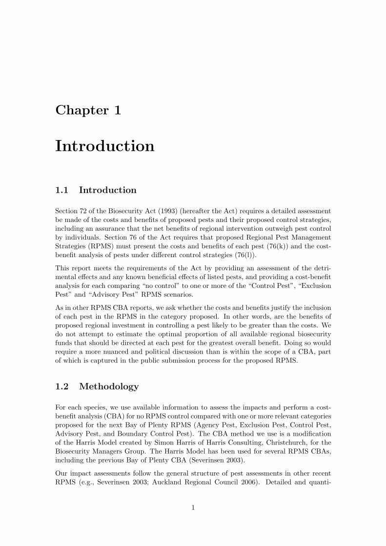
2.1.1 African feather grass (Pennisetum macrourum)
Proposed RPMS Category: Control
Overall impact: Major
Table 2.2: Relevant biology
Attribute DescriptionForm A robust rhizomatous perennial grass up to 1.5 m tall with overhanging
flower spikes which resembles pampas grass. The inflorescence is 10-25cm long, 2 cm in diameter and reddish purple.
Habitat Prefers damp situations such as swamps or stream and lake margins, butgrows in a range of soil types including sand.
Regional distribution Light infestations in the Rotorua area. Isolated in other parts of theregion.
Competitive ability Forms dense clumps that exclude other vegetation.Reproductive ability Seed viability is high but seedling establishment is poor.Dispersal methods Seed dispersed by wind, water, and animals. Also spreads from far
creeping rhizomes and may spread through cultivation with contami-nated machinery.
Resistance to control Readily controlled by appropriate herbicides.
Table 2.3: Impact evaluation
Category Currentimpact
Potentialimpact
Comment Source
Species diversity L M Forms dense clumps and out-competes na-tive pioneer species in many vulnerablehabitats. Also invades established plantcommunities. Can harbour rats, mice andpossums.
1, 2
Threatened species L M 1, 2Soil resources - L Causes accretion of sand and changes in
habitat, leading to erosion or flooding, lossof dunelakes and wetlands.
1
Water quality - L See Soil Resources. 1Production - H Unpalatable to livestock. Fire hazard. 1, 2, 3International trade - M Can contaminate wool. Crop contami-
nant, prohibited seed (nil tolerance) in im-ports into Australia.
1, 4
Human health - - 5Recreation - M Obstructs access to lakes, beaches. 1Maori culture - M Obstructs access to cultural sites (e.g.
waahi tapu, urupa).5
Source: 1: Craw (2000), 2: Environment Bay of Plenty (2005a), 3: Environment Bay of Plenty (2004a),4: Anon. (2009k), 5: Severinsen (2003)
9
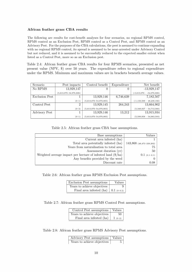
African feather grass CBA results
The following are results for cost-benefit analyses for four scenarios, no regional RPMS control,RPMS control as an Exclusion Pest, RPMS control as a Control Pest, and RPMS control as anAdvisory Pest. For the purposes of the CBA calculations, the pest is assumed to continue expandingwith no regional RPMS control, its spread is assumed to be near-arrested under Advisory Controlbut not reduced, and it is assumed to be successfully reduced to the expected smaller extent whenlisted as a Control Pest, more so as an Exclusion pest.
Table 2.4: African feather grass CBA results for four RPMS scenarios, presented as netpresent value (NPV, $) over 50 years. The expenditure refers to regional expenditureunder the RPMS. Minimum and maximum values are in brackets beneath average values.
Scenario Pest impacts Control benefit Expenditure Net benefitNo RPMS 13,929,147 0 0 -13,929,147
(5,613,070–54,976,806) (-5,613,070 – -54,976,806)
Exclusion Pest 1 13,929,146 6,746,639 7,182,507(0–1) (5,613,070–54,976,805) (-1,133,569 – 48,230,166)
Control Pest 2 13,929,145 264,243 13,664,902(0–3) (5,613,070–54,976,803) (5,348,827 – 54,712,560)
Advisory Pest 1 13,929,146 13,212 13,915,934(0–1) (5,613,070–54,976,805) (5,599,858 – 54,963,593)
Table 2.5: African feather grass CBA base assumptions.
Base assumptions ValuesCurrent area infested (ha) 1
Total area potentially infested (ha) 143,868 (48,473–239,262)
Years from naturalisation to total area 75Assessment duration (yr) 50
Weighted average impact per hectare of infested land ($/ha) 0.1 (0.1–0.1)
Any benefits provided by the weed 0Discount rate 0.08
Table 2.6: African feather grass RPMS Exclusion Pest assumptions.
Exclusion Pest assumptions ValuesYears to achieve objectives 9
Final area infested (ha) 0.1 (0–0.2)
Table 2.7: African feather grass RPMS Control Pest assumptions.
Control Pest assumptions ValuesYears to achieve objectives 50
Final area infested (ha) 1 (0–2)
Table 2.8: African feather grass RPMS Advisory Pest assumptions.
Advisory Pest assumptions ValuesYears to achieve objectives 5
10

Final area infested (ha) 1 (1–2)
Table 2.9: African feather grass estimated total annual cost of di↵erent RPMS scenarios(includes inspection, control, monitoring, enforcement, administration etc.). Subsequentyears are assumed to have the same value as the last year listed.
Exclusion Pest Control Pest Advisory PestYear Total Costs Total Costs Total Costs1.00 1,000,000 20,000 1,000
African feather grass conclusions
In the absence of regional control, the projected total regional damage in net present value is-$13,929,147 over the next 50 years (the minimum projected impact is -$5,613,070).
Managing African feather grass as an Exclusion pest has a projected net benefit to the region of$7,182,507. Since this is positive, this means that this management scenario meets the requirementsof Section 72(1a) of the Act.
Managing African feather grass as a Control pest has a projected net benefit to the region of$13,664,902. Since this is positive, this means that this management scenario meets the require-ments of Section 72(1a) of the Act.
Managing African feather grass as an Advisory pest has a projected net benefit to the region of$13,915,934. Since this is positive, this means that this management scenario meets the require-ments of Section 72(1a) of the Act.
The proposed management scenario for African feather grass, Control, therefore meets the require-ments of Section 72(1a) of the Act.
11

0 20 40 60
0.0
0.2
0.4
0.6
0.8
1.0
Calibrated logistic growth curve, no RPMS control
Years from present
Prop
ortio
n of
max
imum
ext
ent
Current extent (ha): 1
Potential extent (ha): 143,868
(48,473−−239,262)
Time to potential (yr): 75
Current prop. of potential: <0.01
Figure 2.1: The modelled pest spread until it reaches its anticipated maximum extent.Shown are the results of the average (solid line), minimum (dotted line), and maximum(dashed line) scenarios. (A horizontal line means that the pest has already reached itsmaximum extent.) The vertical dotted-dashed lines indicate the CBA assessment periodused in this report.
12

●●
●●
●●
●●
●●
●●
●●
●●
●●
●●
●●
●●
●●
●●
●●
●●
●●
●●
●●
●●
●●
●●
●●
●●
●●
●
010
2030
4050
0
5000
0
1000
00
1500
00
2000
00
Popu
latio
n gr
owth
, no
RPM
S co
ntro
l
Year
s fro
m p
rese
nt
Proportion of initial area
●●
●●
●●
●●
●●
●●
●●
●●
●●
●●
●●
●●
●●
●●
●●
●●
●●
●●
●●
●●
●●
●●
●●
●●
●●
●
010
2030
4050
0
5000
0
1000
00
1500
00
2000
00
Dis
coun
ted
grow
th
Year
s fro
m p
rese
nt
Discounted annual cost
Dis
coun
t rat
e: 0
.08
Tota
l mul
tiplie
r: 54
103.
51
(325
33−−
1605
76)
(a)
●
●
●
●
●
●
●
●
●
●
02
46
8
0.0
0.2
0.4
0.6
0.8
1.0
Popu
latio
n gr
owth
, exc
lusi
on c
ontro
l
Year
s fro
m p
rese
ntProportion of initial area
●
●
●
●
●
●
●
●
●
●
02
46
8
0.0
0.2
0.4
0.6
0.8
1.0
Dis
coun
ted
grow
th, e
xclu
sion
con
trol
Year
s of
con
trol
Discounted annual cost
(b)
●●
●●
●●
●●
●●
●●
●●
●●
●●
●●
●●
●●
●●
●●
●●
●●
●●
●●
●●
●●
●●
●●
●●
●●
●●
●
010
2030
4050
0.0
0.2
0.4
0.6
0.8
1.0
Popu
latio
n gr
owth
, con
trol c
ontro
l
Year
s fro
m p
rese
nt
Proportion of initial area
●
●
●
●
●
●
●
●
●
●
●
●
●
●
●
●
●●
●●
●●
●●
●●
●●
●●
●●
●●
●●
●●
●●
●●
●●
●●
●●
●●
●
010
2030
4050
0.0
0.2
0.4
0.6
0.8
1.0
Dis
coun
ted
grow
th, c
ontro
l con
trol
Year
s of
con
trol
Discounted annual cost
(c)
●
●
●
●
●
●
01
23
45
0.0
0.2
0.4
0.6
0.8
1.0
Popu
latio
n gr
owth
, adv
isor
y co
ntro
l
Year
s fro
m p
rese
nt
Proportion of initial area
●
●
●
●
●
●
01
23
45
0.0
0.2
0.4
0.6
0.8
1.0
Dis
coun
ted
grow
th, a
dvis
ory
cont
rol
Year
s of
con
trol
Discounted annual cost
(d)
Fig
ure
2.2:
The
mod
elle
dpo
pula
tion
chan
ges
over
the
CB
Aas
sess
men
tpe
riod
for
(a)
nore
gion
alco
ntro
l,(b
)E
xclu
sion
Pes
tco
ntro
l,(c
)C
ontr
olPes
tcon
trol
,and
(d)A
dvis
ory
Pes
tcon
trol
.T
heup
perg
raph
ssho
wth
epo
pula
tion
chan
ges,
and
the
low
ergr
aphs
show
the
disc
ount
ing
ofas
soci
ated
impa
cts
each
year
(im
pact
sin
the
futu
rear
eof
less
valu
eec
onom
ical
lyth
anim
pact
sof
the
sam
esi
zeno
w).
13

2.1.2 Alligator weed (Alternanthera philoxeroides)
Proposed RPMS Category: Exclusion
Overall impact: Major
Table 2.10: Relevant biology
Attribute DescriptionForm A floating aquatic, but sometimes terrestrial, perennial herb. Stems
are green-brown, hollow and rooting at nodes. Leaves are obovate tonarrow-elliptical.
Habitat Still water to 1.5 m deep, or flowing fresh water. Tolerates up to 30%sea water. Will grow on moist banks, swampy places, damp pasture anddropping land.
Regional distribution Isolated infestations at Pikowai, Edgecumbe, Te Maunga and Katikati.Competitive ability Floating mats shade out other plants. Biomass doubles in 50 days. Will
out-compete pasture species.Reproductive ability No viable seeds are produced.Dispersal methods Fragments dispersed by cultivation machinery, as weeds or contaminants
of aquatic plant trade.Resistance to control E↵ective control is di�cult, even in small waterways, swampy pastures
and cropping land. Use of herbicide in and beside waterways makescontrol di�cult.
Table 2.11: Impact evaluation
Category Currentimpact
Potentialimpact
Comment Source
Species diversity - H Forms dense mats over water and aroundmargins of waterways. Roots down to 2m deep, replaces most other herbaceousspecies on water and dry land. Rottingvegetation degrades habitat for aquaticfauna and flora.
1
Threatened species - H 1Soil resources - - 1Water quality - M Causes silt accumulation and flooding.
Rotting vegetation degrades water qual-ity.
1
Production L M Can spread from waterways onto croppingland, out-competes other species. Causesphotosensitivity in stock.
1, 2, 3
International trade - - 4Human health - - 4Recreation - H Obstructs access to waterways for fishing,
swimming, kayaking etc.4
Maori culture - L See Recreation. 4Source: 1: Craw (2000), 2: Roy et al. (2004), 3: Environment Bay of Plenty (2004a), 4: Severinsen (2003)
14
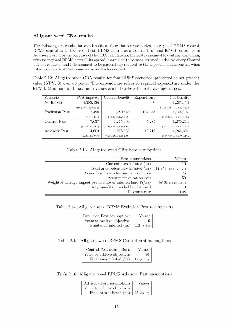
Alligator weed CBA results
The following are results for cost-benefit analyses for four scenarios, no regional RPMS control,RPMS control as an Exclusion Pest, RPMS control as a Control Pest, and RPMS control as anAdvisory Pest. For the purposes of the CBA calculations, the pest is assumed to continue expandingwith no regional RPMS control, its spread is assumed to be near-arrested under Advisory Controlbut not reduced, and it is assumed to be successfully reduced to the expected smaller extent whenlisted as a Control Pest, more so as an Exclusion pest.
Table 2.12: Alligator weed CBA results for four RPMS scenarios, presented as net presentvalue (NPV, $) over 50 years. The expenditure refers to regional expenditure under theRPMS. Minimum and maximum values are in brackets beneath average values.
Scenario Pest impacts Control benefit Expenditure Net benefitNo RPMS 1,283,136 0 0 -1,283,136
(310,129–4,659,531) (-310,129 – -4,659,531)
Exclusion Pest 2,496 1,280,640 134,933 1,145,707(542–4,112) (309,587–4,655,419) (174,654 – 4,520,486)
Control Pest 7,637 1,275,499 5,285 1,270,214(1,445–14,489) (308,684–4,645,042) (303,399 – 4,639,757)
Advisory Pest 4,603 1,278,533 13,212 1,265,321(674–10,506) (309,455–4,649,025) (296,243 – 4,635,813)
Table 2.13: Alligator weed CBA base assumptions.
Base assumptions ValuesCurrent area infested (ha) 10
Total area potentially infested (ha) 12,979 (4,830–21,127)
Years from naturalisation to total area 75Assessment duration (yr) 50
Weighted average impact per hectare of infested land ($/ha) 58.61 (11.72–105.5)
Any benefits provided by the weed 0Discount rate 0.08
Table 2.14: Alligator weed RPMS Exclusion Pest assumptions.
Exclusion Pest assumptions ValuesYears to achieve objectives 9
Final area infested (ha) 1.2 (0–2.5)
Table 2.15: Alligator weed RPMS Control Pest assumptions.
Control Pest assumptions ValuesYears to achieve objectives 50
Final area infested (ha) 12 (15–10)
Table 2.16: Alligator weed RPMS Advisory Pest assumptions.
Advisory Pest assumptions ValuesYears to achieve objectives 5
Final area infested (ha) 25 (35–15)
15

Table 2.17: Alligator weed estimated total annual cost of di↵erent RPMS scenarios (in-cludes inspection, control, monitoring, enforcement, administration etc.). Subsequentyears are assumed to have the same value as the last year listed.
Exclusion Pest Control Pest Advisory PestYear Total Costs Total Costs Total Costs1.00 20,000 400 1,000
Alligator weed conclusions
In the absence of regional control, the projected total regional damage in net present value is-$1,283,136 over the next 50 years (the minimum projected impact is -$310,129).
Managing Alligator weed as an Exclusion pest has a projected net benefit to the region of $1,145,707.Since this is positive, this means that this management scenario meets the requirements of Section72(1a) of the Act.
Managing Alligator weed as a Control pest has a projected net benefit to the region of $1,270,214.Since this is positive, this means that this management scenario meets the requirements of Section72(1a) of the Act.
Managing Alligator weed as an Advisory pest has a projected net benefit to the region of $1,265,321.Since this is positive, this means that this management scenario meets the requirements of Section72(1a) of the Act.
The proposed management scenario for Alligator weed, Exclusion, therefore meets the requirementsof Section 72(1a) of the Act.
16

0 20 40 60
0.0
0.2
0.4
0.6
0.8
1.0
Calibrated logistic growth curve, no RPMS control
Years from present
Prop
ortio
n of
max
imum
ext
ent
Current extent (ha): 10
Potential extent (ha): 12,979
(4,830−−21,127)
Time to potential (yr): 75
Current prop. of potential: 0.001
Figure 2.3: The modelled pest spread until it reaches its anticipated maximum extent.Shown are the results of the average (solid line), minimum (dotted line), and maximum(dashed line) scenarios. (A horizontal line means that the pest has already reached itsmaximum extent.) The vertical dotted-dashed lines indicate the CBA assessment periodused in this report.
17

●●
●●
●●
●●
●●
●●
●●
●●
●●
●●
●●
●●
●●
●●
●●
●●
●●
●●
●●
●●
●●
●●
●●
●●
●●
●
010
2030
4050
0
500
1000
1500
2000
Popu
latio
n gr
owth
, no
RPM
S co
ntro
l
Year
s fro
m p
rese
nt
Proportion of initial area
●●
●●
●●
●●
●●
●●
●●
●●
●●
●●
●●
●●
●●
●●
●●
●●
●●
●●
●●
●●
●●
●●
●●
●●
●●
●
010
2030
4050
0
500
1000
1500
2000
Dis
coun
ted
grow
th
Year
s fro
m p
rese
nt
Discounted annual cost
Dis
coun
t rat
e: 0
.08
Tota
l mul
tiplie
r: 68
8.03
(497−−
1419
)
(a)
●
●
●
●
●
●
●
●
●
●
02
46
8
0.0
0.2
0.4
0.6
0.8
1.0
Popu
latio
n gr
owth
, exc
lusi
on c
ontro
l
Year
s fro
m p
rese
ntProportion of initial area
●
●
●
●
●
●
●
●
●
●
02
46
8
0.0
0.2
0.4
0.6
0.8
1.0
Dis
coun
ted
grow
th, e
xclu
sion
con
trol
Year
s of
con
trol
Discounted annual cost
(b)
●●
●●
●●
●●
●●
●●
●●
●●
●●
●●
●●
●●
●●
●●
●●
●●
●●
●●
●●
●●
●●
●●
●●
●●
●●
●
010
2030
4050
0.0
0.5
1.0
1.5
Popu
latio
n gr
owth
, con
trol c
ontro
l
Year
s fro
m p
rese
nt
Proportion of initial area
●
●
●
●
●
●
●
●
●
●
●
●
●
●
●
●
●●
●●
●●
●●
●●
●●
●●
●●
●●
●●
●●
●●
●●
●●
●●
●●
●●
●
010
2030
4050
0.0
0.2
0.4
0.6
0.8
1.0
Dis
coun
ted
grow
th, c
ontro
l con
trol
Year
s of
con
trol
Discounted annual cost
(c)
●
●
●
●
●
●
01
23
45
0.0
0.5
1.0
1.5
2.0
2.5
3.0
3.5
Popu
latio
n gr
owth
, adv
isor
y co
ntro
l
Year
s fro
m p
rese
nt
Proportion of initial area
●
●
●
●
●
●
01
23
45
0.0
0.2
0.4
0.6
0.8
1.0
Dis
coun
ted
grow
th, a
dvis
ory
cont
rol
Year
s of
con
trol
Discounted annual cost
(d)
Fig
ure
2.4:
The
mod
elle
dpo
pula
tion
chan
ges
over
the
CB
Aas
sess
men
tpe
riod
for
(a)
nore
gion
alco
ntro
l,(b
)E
xclu
sion
Pes
tco
ntro
l,(c
)C
ontr
olPes
tcon
trol
,and
(d)A
dvis
ory
Pes
tcon
trol
.T
heup
perg
raph
ssho
wth
epo
pula
tion
chan
ges,
and
the
low
ergr
aphs
show
the
disc
ount
ing
ofas
soci
ated
impa
cts
each
year
(im
pact
sin
the
futu
rear
eof
less
valu
eec
onom
ical
lyth
anim
pact
sof
the
sam
esi
zeno
w).
18

2.1.3 Apple of Sodom (Solanum linnaeanum)
Proposed RPMS Category: Control
Overall impact: Moderate
Table 2.18: Relevant biology
Attribute DescriptionForm Strongly spiny, woody, perennial shrub up to 1 m tall. Green and white
berries ripen to yellow.Habitat Frost-free coastal areas, poor pasture and scrub margins.Regional distribution Scattered in coastal areas.Competitive ability Can out-compete some species in coastal areas, but does not usually
form pure stands.Reproductive ability Produces viable seed.Dispersal methods Seeds dispersed by birds.Resistance to control Can be controlled with picloram.
Table 2.19: Impact evaluation
Category Currentimpact
Potentialimpact
Comment Source
Species diversity L L Forms dense thickets in coastal areas, ex-cluding low-growing native species.
1
Threatened species - L 1Soil resources - - 2Water quality - - 2Production L M Leaves and unripe fruit are toxic to stock. 1, 3, 4International trade - - 2Human health - M Leaves and unripe fruit are poisonous to
humans.1, 3
Recreation - M Spiny shrub restricts access to beaches. 1, 3Maori culture - M Obstructs access to cultural sites (e.g.
waahi tapu, urupa).1, 3
Source: 1: Craw (2000), 2: Severinsen (2003), 3: Roy et al. (2004), 4: Environment Bay of Plenty (2004a)
19

Apple of Sodom CBA results
The following are results for cost-benefit analyses for four scenarios, no regional RPMS control,RPMS control as an Exclusion Pest, RPMS control as a Control Pest, and RPMS control as anAdvisory Pest. For the purposes of the CBA calculations, the pest is assumed to continue expandingwith no regional RPMS control, its spread is assumed to be near-arrested under Advisory Controlbut not reduced, and it is assumed to be successfully reduced to the expected smaller extent whenlisted as a Control Pest, more so as an Exclusion pest.
Table 2.20: Apple of Sodom CBA results for four RPMS scenarios, presented as net presentvalue (NPV, $) over 50 years. The expenditure refers to regional expenditure under theRPMS. Minimum and maximum values are in brackets beneath average values.
Scenario Pest impacts Control benefit Expenditure Net benefitNo RPMS 1,125,267 0 0 -1,125,267
(257,779–3,043,407) (-257,779 – -3,043,407)
Exclusion Pest 15,317 1,109,950 6,746,639 -5,636,689(3,136–25,392) (254,643–3,018,015) (-6,491,996 – -3,728,624)
Control Pest 42,820 1,082,447 66,061 1,016,386(8,274–75,724) (249,505–2,967,683) (183,444 – 2,901,622)
Advisory Pest 28,247 1,097,020 13,212 1,083,808(3,903–64,873) (253,876–2,978,534) (240,664 – 2,965,322)
Table 2.21: Apple of Sodom CBA base assumptions.
Base assumptions ValuesCurrent area infested (ha) 78
Total area potentially infested (ha) 55,049 (19,374–90,723)
Years from naturalisation to total area 125Assessment duration (yr) 50
Weighted average impact per hectare of infested land ($/ha) 46.11 (8.7–83.52)
Any benefits provided by the weed 0Discount rate 0.08
Table 2.22: Apple of Sodom RPMS Exclusion Pest assumptions.
Exclusion Pest assumptions ValuesYears to achieve objectives 9
Final area infested (ha) 9.8 (0–19.5)
Table 2.23: Apple of Sodom RPMS Control Pest assumptions.
Control Pest assumptions ValuesYears to achieve objectives 50
Final area infested (ha) 66 (58–74)
Table 2.24: Apple of Sodom RPMS Advisory Pest assumptions.
Advisory Pest assumptions ValuesYears to achieve objectives 5
Final area infested (ha) 195 (273–117)
20

Table 2.25: Apple of Sodom estimated total annual cost of di↵erent RPMS scenarios(includes inspection, control, monitoring, enforcement, administration etc.). Subsequentyears are assumed to have the same value as the last year listed.
Exclusion Pest Control Pest Advisory PestYear Total Costs Total Costs Total Costs1.00 1,000,000 5,000 1,000
Apple of Sodom conclusions
In the absence of regional control, the projected total regional damage in net present value is-$1,125,267 over the next 50 years (the minimum projected impact is -$257,779).
Managing Apple of Sodom as an Exclusion pest has a projected net benefit to the region of -$5,636,689. Since this is negative, this means that this management scenario does not meets therequirements of Section 72(1a) of the Act.
Managing Apple of Sodom as a Control pest has a projected net benefit to the region of $1,016,386.Since this is positive, this means that this management scenario meets the requirements of Section72(1a) of the Act.
Managing Apple of Sodom as an Advisory pest has a projected net benefit to the region of$1,083,808. Since this is positive, this means that this management scenario meets the requirementsof Section 72(1a) of the Act.
The proposed management scenario for Apple of Sodom, Control, therefore meets the requirementsof Section 72(1a) of the Act.
21

0 20 40 60 80 100 120
0.0
0.2
0.4
0.6
0.8
1.0
Calibrated logistic growth curve, no RPMS control
Years from present
Prop
ortio
n of
max
imum
ext
ent
Current extent (ha): 78
Potential extent (ha): 55,049
(19,374−−90,723)
Time to potential (yr): 125
Current prop. of potential: 0.002
Figure 2.5: The modelled pest spread until it reaches its anticipated maximum extent.Shown are the results of the average (solid line), minimum (dotted line), and maximum(dashed line) scenarios. (A horizontal line means that the pest has already reached itsmaximum extent.) The vertical dotted-dashed lines indicate the CBA assessment periodused in this report.
22

●●
●●
●●
●●
●●
●●
●●
●●
●●
●●
●●
●●
●●
●●
●●
●●
●●
●●
●●
●●
●
●
●
●
●
●
●
●
●
●
●
010
2030
4050
050100
150
200
250
Popu
latio
n gr
owth
, no
RPM
S co
ntro
l
Year
s fro
m p
rese
nt
Proportion of initial area
●●
●●
●●
●●
●●
●●
●●
●●
●●
●●
●●
●●
●●
●●
●●
●●
●●
●●
●●
●●
●●
●●
●●
●●
●●
●
010
2030
4050
050100
150
200
250
Dis
coun
ted
grow
th
Year
s fro
m p
rese
nt
Discounted annual cost
Dis
coun
t rat
e: 0
.08
Tota
l mul
tiplie
r: 10
8.15
(92−−1
49)
(a)
●
●
●
●
●
●
●
●
●
●
02
46
8
0.0
0.2
0.4
0.6
0.8
1.0
Popu
latio
n gr
owth
, exc
lusi
on c
ontro
l
Year
s fro
m p
rese
ntProportion of initial area
●
●
●
●
●
●
●
●
●
●
02
46
8
0.0
0.2
0.4
0.6
0.8
1.0
Dis
coun
ted
grow
th, e
xclu
sion
con
trol
Year
s of
con
trol
Discounted annual cost
(b)
●●
●●
●●
●●
●●
●●
●●
●●
●●
●●
●●
●●
●●
●●
●●
●●
●●
●●
●●
●●
●●
●●
●●
●●
●●
●
010
2030
4050
0.0
0.2
0.4
0.6
0.8
1.0
Popu
latio
n gr
owth
, con
trol c
ontro
l
Year
s fro
m p
rese
nt
Proportion of initial area
●
●
●
●
●
●
●
●
●
●
●
●
●
●
●
●●
●●
●●
●●
●●
●●
●●
●●
●●
●●
●●
●●
●●
●●
●●
●●
●●
●●
010
2030
4050
0.0
0.2
0.4
0.6
0.8
1.0
Dis
coun
ted
grow
th, c
ontro
l con
trol
Year
s of
con
trol
Discounted annual cost
(c)
●
●
●
●
●
●
01
23
45
0.0
0.5
1.0
1.5
2.0
2.5
3.0
3.5
Popu
latio
n gr
owth
, adv
isor
y co
ntro
l
Year
s fro
m p
rese
nt
Proportion of initial area
●
●
●
●
●
●
01
23
45
0.0
0.2
0.4
0.6
0.8
1.0
Dis
coun
ted
grow
th, a
dvis
ory
cont
rol
Year
s of
con
trol
Discounted annual cost
(d)
Fig
ure
2.6:
The
mod
elle
dpo
pula
tion
chan
ges
over
the
CB
Aas
sess
men
tpe
riod
for
(a)
nore
gion
alco
ntro
l,(b
)E
xclu
sion
Pes
tco
ntro
l,(c
)C
ontr
olPes
tcon
trol
,and
(d)A
dvis
ory
Pes
tcon
trol
.T
heup
perg
raph
ssho
wth
epo
pula
tion
chan
ges,
and
the
low
ergr
aphs
show
the
disc
ount
ing
ofas
soci
ated
impa
cts
each
year
(im
pact
sin
the
futu
rear
eof
less
valu
eec
onom
ical
lyth
anim
pact
sof
the
sam
esi
zeno
w).
23

2.1.4 Asiatic knotweed (Reynoutria japonica)
Proposed RPMS Category: Control
Overall impact: Major
Table 2.26: Relevant biology
Attribute DescriptionForm Thicket forming, rhizomatous herb up to 2 m tall.Habitat Roadsides, riverbanks and waste places.Regional distribution Rotorua area, Te Puke area.Competitive ability Can be competitive in localised areas.Reproductive ability Produces viable seed.Dispersal methods Water, contaminated soil. Also spreads by rhizomes.Resistance to control Can be controlled with herbicides.
Table 2.27: Impact evaluation
Category Currentimpact
Potentialimpact
Comment Source
Species diversity L H Forms dense, long-lived thickets, excludesother species, prevents recruitment.
1, 2
Threatened species - H 1, 2Soil resources - L 3Water quality - H Blocks up waterways. 3Production - M Forms dense, long-lived thickets, excludes
other species.1, 2
International trade - - 4Human health - - 4Recreation - H Obstructs access to waterways for fishing,
swimming, kayaking etc.3
Maori culture - H See Recreation. 3Source: 1: Craw (2000), 2: Environment Bay of Plenty (2005b), 3: Senior (2009), 4: Severinsen (2003)
24

Asiatic knotweed CBA results
The following are results for cost-benefit analyses for four scenarios, no regional RPMS control,RPMS control as an Exclusion Pest, RPMS control as a Control Pest, and RPMS control as anAdvisory Pest. For the purposes of the CBA calculations, the pest is assumed to continue expandingwith no regional RPMS control, its spread is assumed to be near-arrested under Advisory Controlbut not reduced, and it is assumed to be successfully reduced to the expected smaller extent whenlisted as a Control Pest, more so as an Exclusion pest.
Table 2.28: Asiatic knotweed CBA results for four RPMS scenarios, presented as netpresent value (NPV, $) over 50 years. The expenditure refers to regional expenditureunder the RPMS. Minimum and maximum values are in brackets beneath average values.
Scenario Pest impacts Control benefit Expenditure Net benefitNo RPMS 1,170,331 0 0 -1,170,331
(320,671–5,348,647) (-320,671 – -5,348,647)
Exclusion Pest 12 1,170,319 5,059,979 -3,889,660(2–19) (320,669–5,348,628) (-4,739,310 – 288,649)
Control Pest 31 1,170,300 198,182 972,118(6–54) (320,665–5,348,593) (122,483 – 5,150,411)
Advisory Pest 14 1,170,317 13,212 1,157,105(3–23) (320,668–5,348,624) (307,456 – 5,335,412)
Table 2.29: Asiatic knotweed CBA base assumptions.
Base assumptions ValuesCurrent area infested (ha) 6
Total area potentially infested (ha) 103,636 (35,026–172,246)
Years from naturalisation to total area 75Assessment duration (yr) 50
Weighted average impact per hectare of infested land ($/ha) 0.1 (0.1–0.83)
Any benefits provided by the weed 0Discount rate 0.08
Table 2.30: Asiatic knotweed RPMS Exclusion Pest assumptions.
Exclusion Pest assumptions ValuesYears to achieve objectives 9
Final area infested (ha) 0.7 (0–1.5)
Table 2.31: Asiatic knotweed RPMS Control Pest assumptions.
Control Pest assumptions ValuesYears to achieve objectives 50
Final area infested (ha) 4 (3–4)
Table 2.32: Asiatic knotweed RPMS Advisory Pest assumptions.
Advisory Pest assumptions ValuesYears to achieve objectives 5
25

Final area infested (ha) 8 (6–9)
Table 2.33: Asiatic knotweed estimated total annual cost of di↵erent RPMS scenarios(includes inspection, control, monitoring, enforcement, administration etc.). Subsequentyears are assumed to have the same value as the last year listed.
Exclusion Pest Control Pest Advisory PestYear Total Costs Total Costs Total Costs1.00 750,000 15,000 1,000
Asiatic knotweed conclusions
In the absence of regional control, the projected total regional damage in net present value is-$1,170,331 over the next 50 years (the minimum projected impact is -$320,671).
Managing Asiatic knotweed as an Exclusion pest has a projected net benefit to the region of -$3,889,660. Since this is negative, this means that this management scenario does not meets therequirements of Section 72(1a) of the Act.
Managing Asiatic knotweed as a Control pest has a projected net benefit to the region of $972,118.Since this is positive, this means that this management scenario meets the requirements of Section72(1a) of the Act.
Managing Asiatic knotweed as an Advisory pest has a projected net benefit to the region of$1,157,105. Since this is positive, this means that this management scenario meets the requirementsof Section 72(1a) of the Act.
The proposed management scenario for Asiatic knotweed, Control, therefore meets the require-ments of Section 72(1a) of the Act.
26

0 20 40 60
0.0
0.2
0.4
0.6
0.8
1.0
Calibrated logistic growth curve, no RPMS control
Years from present
Prop
ortio
n of
max
imum
ext
ent
Current extent (ha): 6
Potential extent (ha): 103,636
(35,026−−172,246)
Time to potential (yr): 75
Current prop. of potential: <0.01
Figure 2.7: The modelled pest spread until it reaches its anticipated maximum extent.Shown are the results of the average (solid line), minimum (dotted line), and maximum(dashed line) scenarios. (A horizontal line means that the pest has already reached itsmaximum extent.) The vertical dotted-dashed lines indicate the CBA assessment periodused in this report.
27

●●
●●
●●
●●
●●
●●
●●
●●
●●
●●
●●
●●
●●
●●
●●
●●
●●
●●
●●
●●
●●
●●
●●
●●
●●
●
010
2030
4050
0
5000
1000
0
1500
0
2000
0
2500
0
Popu
latio
n gr
owth
, no
RPM
S co
ntro
l
Year
s fro
m p
rese
nt
Proportion of initial area
●●
●●
●●
●●
●●
●●
●●
●●
●●
●●
●●
●●
●●
●●
●●
●●
●●
●●
●●
●●
●●
●●
●●
●●
●●
●
010
2030
4050
0
5000
1000
0
1500
0
2000
0
2500
0
Dis
coun
ted
grow
th
Year
s fro
m p
rese
nt
Discounted annual cost
Dis
coun
t rat
e: 0
.08
Tota
l mul
tiplie
r: 65
12.5
2
(391
9−−1
9267
)
(a)
●
●
●
●
●
●
●
●
●
●
02
46
8
0.0
0.2
0.4
0.6
0.8
1.0
Popu
latio
n gr
owth
, exc
lusi
on c
ontro
l
Year
s fro
m p
rese
ntProportion of initial area
●
●
●
●
●
●
●
●
●
●
02
46
8
0.0
0.2
0.4
0.6
0.8
1.0
Dis
coun
ted
grow
th, e
xclu
sion
con
trol
Year
s of
con
trol
Discounted annual cost
(b)
●●
●●
●●
●●
●●
●●
●●
●●
●●
●●
●●
●●
●●
●●
●●
●●
●●
●●
●●
●●
●●
●●
●●
●●
●●
●
010
2030
4050
0.0
0.2
0.4
0.6
0.8
1.0
Popu
latio
n gr
owth
, con
trol c
ontro
l
Year
s fro
m p
rese
nt
Proportion of initial area
●
●
●
●
●
●
●
●
●
●
●
●
●
●
●
●●
●●
●●
●●
●●
●●
●●
●●
●●
●●
●●
●●
●●
●●
●●
●●
●●
●●
010
2030
4050
0.0
0.2
0.4
0.6
0.8
1.0
Dis
coun
ted
grow
th, c
ontro
l con
trol
Year
s of
con
trol
Discounted annual cost
(c)
●
●
●
●
●
●
01
23
45
0.0
0.2
0.4
0.6
0.8
1.0
Popu
latio
n gr
owth
, adv
isor
y co
ntro
l
Year
s fro
m p
rese
nt
Proportion of initial area
●
●
●
●
●
●
01
23
45
0.0
0.2
0.4
0.6
0.8
1.0
Dis
coun
ted
grow
th, a
dvis
ory
cont
rol
Year
s of
con
trol
Discounted annual cost
(d)
Fig
ure
2.8:
The
mod
elle
dpo
pula
tion
chan
ges
over
the
CB
Aas
sess
men
tpe
riod
for
(a)
nore
gion
alco
ntro
l,(b
)E
xclu
sion
Pes
tco
ntro
l,(c
)C
ontr
olPes
tcon
trol
,and
(d)A
dvis
ory
Pes
tcon
trol
.T
heup
perg
raph
ssho
wth
epo
pula
tion
chan
ges,
and
the
low
ergr
aphs
show
the
disc
ount
ing
ofas
soci
ated
impa
cts
each
year
(im
pact
sin
the
futu
rear
eof
less
valu
eec
onom
ical
lyth
anim
pact
sof
the
sam
esi
zeno
w).
28

2.1.5 Banana passionfruit (Passiflora tripartita var.mollissima, P. tarmini-ana, P. caerulea)
Proposed RPMS Category: Advisory
Overall impact: Moderate
Table 2.34: Relevant biology
Attribute DescriptionForm Vigorous high climbing vine. Three-lobed leaves large hanging pink star-
shaped flowers, which become a yellow oval fruit.Habitat Margins of forest, wind breaks, orchard shelterbelts, usually close to
habitation. Also on roadsides, wasteland and open coastal forest.Regional distribution Found in all parts of the region.Competitive ability Plants are shade intolerant but tolerant of physical damage and graz-
ing. In wet areas damage by fungus, Pythiums and slugs may decreaseestablishment success. Very rapid growth rate. Seeds require high lightfor germination.
Reproductive ability Low percentage of seeds develop to maturity, but if a pollinator wereintroduced this rate would increase dramatically.
Dispersal methods Dispersed by possums and birds that peck at fallen fruit. Overseasevidence shows mainly dispersed by pigs, cattle and pheasants. Alsospread by humans who discard partly eaten fruit or who grow it for itsfruit.
Resistance to control Plants can be hand-pulled when young but regrowth needs to besprayed with 2% glyphosate. Biocontrol possibilities being investigatedin Hawaii.
Benefits Edible fruit.
Table 2.35: Impact evaluation
Category Currentimpact
Potentialimpact
Comment Source
Species diversity L H Smothers canopy, prevents recruitment.Allows faster-growing or tougher vines tosucceed it in dominating canopy.
1, 2
Threatened species L M 1, 2Soil resources - - 3Water quality - - 3Production - L Smothers trees in plantation forests, cre-
ates safety hazard during harvest of plan-tation trees.
1, 4, 5
International trade - - 3Human health - - 3Recreation - L Dense walls of vines obstruct access to for-
est.3
Maori culture - L See Recreation. 3Source: 1: Craw (2000), 2: Williams & Buxton (1995), 3: Severinsen (2003), 4: Roy et al. (2004), 5:
Anon. (2007a)
29

Banana passionfruit CBA results
The following are results for cost-benefit analyses for four scenarios, no regional RPMS control,RPMS control as an Exclusion Pest, RPMS control as a Control Pest, and RPMS control as anAdvisory Pest. For the purposes of the CBA calculations, the pest is assumed to continue expandingwith no regional RPMS control, its spread is assumed to be near-arrested under Advisory Controlbut not reduced, and it is assumed to be successfully reduced to the expected smaller extent whenlisted as a Control Pest, more so as an Exclusion pest.
Table 2.36: Banana passionfruit CBA results for four RPMS scenarios, presented as netpresent value (NPV, $) over 50 years. The expenditure refers to regional expenditureunder the RPMS. Minimum and maximum values are in brackets beneath average values.
Scenario Pest impacts Control benefit Expenditure Net benefitNo RPMS 86,588 0 0 -86,588
(29,167–373,714) (-29,167 – -373,714)
Exclusion Pest 39 86,549 6,746,639 -6,660,090(8–65) (29,159–373,649) (-6,717,480 – -6,372,990)
Control Pest 111 86,477 264,243 -177,766(22–194) (29,145–373,520) (-235,098 – 109,277)
Advisory Pest 51 86,537 26,424 60,113(9–96) (29,158–373,618) (2,734 – 347,194)
Table 2.37: Banana passionfruit CBA base assumptions.
Base assumptions ValuesCurrent area infested (ha) 20
Total area potentially infested (ha) 99,372 (33,602–165,143)
Years from naturalisation to total area 100Assessment duration (yr) 50
Weighted average impact per hectare of infested land ($/ha) 0.1 (0.1–0.83)
Any benefits provided by the weed 0Discount rate 0.08
Table 2.38: Banana passionfruit RPMS Exclusion Pest assumptions.
Exclusion Pest assumptions ValuesYears to achieve objectives 9
Final area infested (ha) 2.5 (0–5)
Table 2.39: Banana passionfruit RPMS Control Pest assumptions.
Control Pest assumptions ValuesYears to achieve objectives 50
Final area infested (ha) 18 (15–20)
Table 2.40: Banana passionfruit RPMS Advisory Pest assumptions.
Advisory Pest assumptions ValuesYears to achieve objectives 5
30

Final area infested (ha) 28 (30–25)
Table 2.41: Banana passionfruit estimated total annual cost of di↵erent RPMS scenarios(includes inspection, control, monitoring, enforcement, administration etc.). Subsequentyears are assumed to have the same value as the last year listed.
Exclusion Pest Control Pest Advisory PestYear Total Costs Total Costs Total Costs1.00 1,000,000 20,000 2,000
Banana passionfruit conclusions
In the absence of regional control, the projected total regional damage in net present value is-$86,588 over the next 50 years (the minimum projected impact is -$29,167).
Managing Banana passionfruit as an Exclusion pest has a projected net benefit to the region of-$6,660,090. Since this is negative, this means that this management scenario does not meets therequirements of Section 72(1a) of the Act.
Managing Banana passionfruit as a Control pest has a projected net benefit to the region of -$177,766. Since this is negative, this means that this management scenario does not meet therequirements of Section 72(1a) of the Act.
Managing Banana passionfruit as an Advisory pest has a projected net benefit to the region of$60,113. Since this is positive, this means that this management scenario meets the requirementsof Section 72(1a) of the Act.
The proposed management scenario for Banana passionfruit, Advisory, therefore meets the require-ments of Section 72(1a) of the Act.
31

0 20 40 60 80 100
0.0
0.2
0.4
0.6
0.8
1.0
Calibrated logistic growth curve, no RPMS control
Years from present
Prop
ortio
n of
max
imum
ext
ent
Current extent (ha): 20
Potential extent (ha): 99,372
(33,602−−165,143)
Time to potential (yr): 100
Current prop. of potential: <0.01
Figure 2.9: The modelled pest spread until it reaches its anticipated maximum extent.Shown are the results of the average (solid line), minimum (dotted line), and maximum(dashed line) scenarios. (A horizontal line means that the pest has already reached itsmaximum extent.) The vertical dotted-dashed lines indicate the CBA assessment periodused in this report.
32

●●
●●
●●
●●
●●
●●
●●
●●
●●
●●
●●
●●
●●
●●
●●
●●
●●
●●
●●
●●
●●
●●
●●
●
●
●
●
●
010
2030
4050
0
1000
2000
3000
4000
Popu
latio
n gr
owth
, no
RPM
S co
ntro
l
Year
s fro
m p
rese
nt
Proportion of initial area
●●
●●
●●
●●
●●
●●
●●
●●
●●
●●
●●
●●
●●
●●
●●
●●
●●
●●
●●
●●
●●
●●
●●
●●
●●
●
010
2030
4050
0
1000
2000
3000
4000
Dis
coun
ted
grow
th
Year
s fro
m p
rese
nt
Discounted annual cost
Dis
coun
t rat
e: 0
.08
Tota
l mul
tiplie
r: 63
6.91
(399−−
1882
)
(a)
●
●
●
●
●
●
●
●
●
●
02
46
8
0.0
0.2
0.4
0.6
0.8
1.0
Popu
latio
n gr
owth
, exc
lusi
on c
ontro
l
Year
s fro
m p
rese
ntProportion of initial area
●
●
●
●
●
●
●
●
●
●
02
46
8
0.0
0.2
0.4
0.6
0.8
1.0
Dis
coun
ted
grow
th, e
xclu
sion
con
trol
Year
s of
con
trol
Discounted annual cost
(b)
●●
●●
●●
●●
●●
●●
●●
●●
●●
●●
●●
●●
●●
●●
●●
●●
●●
●●
●●
●●
●●
●●
●●
●●
●●
●
010
2030
4050
0.0
0.2
0.4
0.6
0.8
1.0
Popu
latio
n gr
owth
, con
trol c
ontro
l
Year
s fro
m p
rese
nt
Proportion of initial area
●
●
●
●
●
●
●
●
●
●
●
●
●
●
●
●●
●●
●●
●●
●●
●●
●●
●●
●●
●●
●●
●●
●●
●●
●●
●●
●●
●●
010
2030
4050
0.0
0.2
0.4
0.6
0.8
1.0
Dis
coun
ted
grow
th, c
ontro
l con
trol
Year
s of
con
trol
Discounted annual cost
(c)
●
●
●
●
●
●
01
23
45
0.0
0.5
1.0
1.5
Popu
latio
n gr
owth
, adv
isor
y co
ntro
l
Year
s fro
m p
rese
nt
Proportion of initial area
●
●●
●●
●
01
23
45
0.0
0.2
0.4
0.6
0.8
1.0
Dis
coun
ted
grow
th, a
dvis
ory
cont
rol
Year
s of
con
trol
Discounted annual cost
(d)
Fig
ure
2.10
:T
hem
odel
led
popu
lati
onch
ange
sov
erth
eC
BA
asse
ssm
ent
peri
odfo
r(a
)no
regi
onal
cont
rol,
(b)
Exc
lusi
onPes
tco
ntro
l,(c
)C
ontr
olPes
tco
ntro
l,an
d(d
)A
dvis
ory
Pes
tco
ntro
l.T
heup
per
grap
hssh
owth
epo
pula
tion
chan
ges,
and
the
low
ergr
aphs
show
the
disc
ount
ing
ofas
soci
ated
impa
cts
each
year
(im
pact
sin
the
futu
rear
eof
less
valu
eec
onom
ical
lyth
anim
pact
sof
the
sam
esi
zeno
w).
33
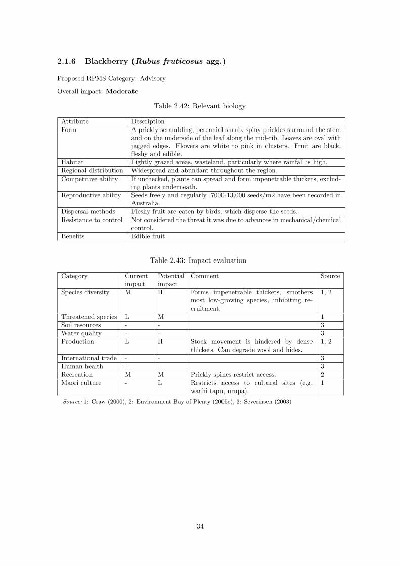
2.1.6 Blackberry (Rubus fruticosus agg.)
Proposed RPMS Category: Advisory
Overall impact: Moderate
Table 2.42: Relevant biology
Attribute DescriptionForm A prickly scrambling, perennial shrub, spiny prickles surround the stem
and on the underside of the leaf along the mid-rib. Leaves are oval withjagged edges. Flowers are white to pink in clusters. Fruit are black,fleshy and edible.
Habitat Lightly grazed areas, wasteland, particularly where rainfall is high.Regional distribution Widespread and abundant throughout the region.Competitive ability If unchecked, plants can spread and form impenetrable thickets, exclud-
ing plants underneath.Reproductive ability Seeds freely and regularly. 7000-13,000 seeds/m2 have been recorded in
Australia.Dispersal methods Fleshy fruit are eaten by birds, which disperse the seeds.Resistance to control Not considered the threat it was due to advances in mechanical/chemical
control.Benefits Edible fruit.
Table 2.43: Impact evaluation
Category Currentimpact
Potentialimpact
Comment Source
Species diversity M H Forms impenetrable thickets, smothersmost low-growing species, inhibiting re-cruitment.
1, 2
Threatened species L M 1Soil resources - - 3Water quality - - 3Production L H Stock movement is hindered by dense
thickets. Can degrade wool and hides.1, 2
International trade - - 3Human health - - 3Recreation M M Prickly spines restrict access. 2Maori culture - L Restricts access to cultural sites (e.g.
waahi tapu, urupa).1
Source: 1: Craw (2000), 2: Environment Bay of Plenty (2005c), 3: Severinsen (2003)
34

Blackberry CBA results
The following are results for cost-benefit analyses for four scenarios, no regional RPMS control,RPMS control as an Exclusion Pest, RPMS control as a Control Pest, and RPMS control as anAdvisory Pest. For the purposes of the CBA calculations, the pest is assumed to continue expandingwith no regional RPMS control, its spread is assumed to be near-arrested under Advisory Controlbut not reduced, and it is assumed to be successfully reduced to the expected smaller extent whenlisted as a Control Pest, more so as an Exclusion pest.
Table 2.44: Blackberry CBA results for four RPMS scenarios, presented as net presentvalue (NPV, $) over 50 years. The expenditure refers to regional expenditure under theRPMS. Minimum and maximum values are in brackets beneath average values.
Scenario Pest impacts Control benefit Expenditure Net benefitNo RPMS 1,439,329,161 0 0 -1,439,329,161
(497,445,080–886,721,947) (-497,445,080 – -886,721,947)
Exclusion Pest 63,453,398 1,375,875,763 21,707,311 1,354,168,452(14,364,018–104,035,028) (483,081,062–782,686,919) (461,373,751 – 760,979,608)
Control Pest 167,966,470 1,271,362,691 850,203 1,270,512,488(36,145,907–291,499,519) (461,299,173–595,222,428) (460,448,970 – 594,372,225)
Advisory Pest 69,984,400 1,369,344,761 13,212 1,369,331,549(14,605,109–125,363,690) (482,839,971–761,358,257) (482,826,759 – 761,345,045)
Table 2.45: Blackberry CBA base assumptions.
Base assumptions ValuesCurrent area infested (ha) 611,065
Total area potentially infested (ha) 139,509 (47,022–231,995)
Years from naturalisation to total area 100Assessment duration (yr) 50
Weighted average impact per hectare of infested land ($/ha) 24.38 (5.09–43.68)
Any benefits provided by the weed 0Discount rate 0.08
Table 2.46: Blackberry RPMS Exclusion Pest assumptions.
Exclusion Pest assumptions ValuesYears to achieve objectives 9
Final area infested (ha) 76,383.1 (0–152,766.2)
Table 2.47: Blackberry RPMS Control Pest assumptions.
Control Pest assumptions ValuesYears to achieve objectives 50
Final area infested (ha) 381,916 (305,532–458,299)
Table 2.48: Blackberry RPMS Advisory Pest assumptions.
Advisory Pest assumptions ValuesYears to achieve objectives 5
Final area infested (ha) 611,065 (611,065–611,065)
35

Table 2.49: Blackberry estimated total annual cost of di↵erent RPMS scenarios (includesinspection, control, monitoring, enforcement, administration etc.). Subsequent years areassumed to have the same value as the last year listed.
Exclusion Pest Control Pest Advisory PestYear Total Costs Total Costs Total Costs1.00 3,217,500 64,350 1,000
Blackberry conclusions
In the absence of regional control, the projected total regional damage in net present value is-$1,439,329,161 over the next 50 years (the minimum projected impact is -$497,445,080).
Managing Blackberry as an Exclusion pest has a projected net benefit to the region of $1,354,168,452.Since this is positive, this means that this management scenario meets the requirements of Section72(1a) of the Act.
Managing Blackberry as a Control pest has a projected net benefit to the region of $1,270,512,488.Since this is positive, this means that this management scenario meets the requirements of Section72(1a) of the Act.
Managing Blackberry as an Advisory pest has a projected net benefit to the region of $1,369,331,549.Since this is positive, this means that this management scenario meets the requirements of Section72(1a) of the Act.
The proposed management scenario for Blackberry, Advisory, therefore meets the requirements ofSection 72(1a) of the Act.
36
0 10 20 30 40 50
0.0
0.2
0.4
0.6
0.8
1.0
Calibrated logistic growth curve
Years from present
Prop
ortio
n of
max
imum
ext
ent
Figure 2.11: The modelled pest spread until it reaches its anticipated maximum extent.Shown are the results of the average (solid line), minimum (dotted line), and maximum(dashed line) scenarios. (A horizontal line means that the pest has already reached itsmaximum extent.) The vertical dotted-dashed lines indicate the CBA assessment periodused in this report.
37

● 010
2030
4050
1.0
1.5
2.0
2.5
Popu
latio
n gr
owth
, no
RPM
S co
ntro
l
Year
s fro
m p
rese
nt
Proportion of initial area
●
●
●
●
●
●
●
●
●
●
●
●
●
●
●
●
●
●
●
●
●
●
●
●
●
●
●
●
●
●
●
●●
●●
●●
●●
●●
●●
●●
●●
●●
●●
010
2030
4050
0.0
0.5
1.0
1.5
2.0
2.5
Dis
coun
ted
grow
th
Year
s fro
m p
rese
nt
Discounted annual cost
Dis
coun
t rat
e: 0
.08
Tota
l mul
tiplie
r: 96
.6
(160−−
33)
(a)
●
●
●
●
●
●
●
●
●
●
02
46
8
0.0
0.2
0.4
0.6
0.8
1.0
Popu
latio
n gr
owth
, exc
lusi
on c
ontro
l
Year
s fro
m p
rese
ntProportion of initial area
●
●
●
●
●
●
●
●
●
●
02
46
8
0.0
0.2
0.4
0.6
0.8
1.0
Dis
coun
ted
grow
th, e
xclu
sion
con
trol
Year
s of
con
trol
Discounted annual cost
(b)
●●
●●
●●
●●
●●
●●
●●
●●
●●
●●
●●
●●
●●
●●
●●
●●
●●
●●
●●
●●
●●
●●
●●
●●
●●
●
010
2030
4050
0.0
0.2
0.4
0.6
0.8
1.0
Popu
latio
n gr
owth
, con
trol c
ontro
l
Year
s fro
m p
rese
nt
Proportion of initial area
●
●
●
●
●
●
●
●
●
●
●
●
●
●
●
●●
●●
●●
●●
●●
●●
●●
●●
●●
●●
●●
●●
●●
●●
●●
●●
●●
●●
010
2030
4050
0.0
0.2
0.4
0.6
0.8
1.0
Dis
coun
ted
grow
th, c
ontro
l con
trol
Year
s of
con
trol
Discounted annual cost
(c)
●●
●●
●●
01
23
45
0.0
0.2
0.4
0.6
0.8
1.0
Popu
latio
n gr
owth
, adv
isor
y co
ntro
l
Year
s fro
m p
rese
nt
Proportion of initial area
●
●
●
●
●
●
01
23
45
0.0
0.2
0.4
0.6
0.8
1.0
Dis
coun
ted
grow
th, a
dvis
ory
cont
rol
Year
s of
con
trol
Discounted annual cost
(d)
Fig
ure
2.12
:T
hem
odel
led
popu
lati
onch
ange
sov
erth
eC
BA
asse
ssm
ent
peri
odfo
r(a
)no
regi
onal
cont
rol,
(b)
Exc
lusi
onPes
tco
ntro
l,(c
)C
ontr
olPes
tco
ntro
l,an
d(d
)A
dvis
ory
Pes
tco
ntro
l.T
heup
per
grap
hssh
owth
epo
pula
tion
chan
ges,
and
the
low
ergr
aphs
show
the
disc
ount
ing
ofas
soci
ated
impa
cts
each
year
(im
pact
sin
the
futu
rear
eof
less
valu
eec
onom
ical
lyth
anim
pact
sof
the
sam
esi
zeno
w).
38

2.1.7 Boneseed (Chrysanthemoides monilifera)
Proposed RPMS Category: Control
Overall impact: Major
Table 2.50: Relevant biology
Attribute DescriptionForm Bushy, much branched shrub growing to 3 m tall.Habitat Coastal cli↵s, waste places, consolidated dunes and scrubland.Regional distribution Isolated infestations along the coast.Competitive ability Plants are tolerant of low fertility and drought, but intolerant of shade
and wet. Plant is fire-adapted with seed germination stimulated by fireevents. Fast shoot growth. Can spread by layering, forming pure stands.
Reproductive ability 5000 seeds produced per plant, viable for up to 10 years.Dispersal methods Birds disperse seeds.Resistance to control Tolerant of some physical damage. Can be controlled with brush weed
killers but leaves a large seed bank. This plant is the highest priority forbiological control in Australia.
Table 2.51: Impact evaluation
Category Currentimpact
Potentialimpact
Comment Source
Species diversity M H Colonises disturbed sites faster than na-tive species, rapidly replaces other speciesunder 2 m, prevents recruitment. Createsheavy shade where high light levels shouldoccur.
1, 2
Threatened species L H Could threaten rare coastal shrubs. 1Soil resources L L Causes erosion. 3, 4Water quality - - 5Production L L Forms dense impenetrable stands. 5International trade - - 5Human health - L Highly flammable. Fire risk near housing. 5Recreation L L Dense stands obstruct access in coastal ar-
eas.2
Maori culture L M A nuisance at Te Whare pa near Ohope. 3, 5Source: 1: Craw (2000), 2: ECan (2003), 3: Mather (2009), 4: Stahl (2009), 5: Severinsen (2003)
39

Boneseed CBA results
The following are results for cost-benefit analyses for four scenarios, no regional RPMS control,RPMS control as an Exclusion Pest, RPMS control as a Control Pest, and RPMS control as anAdvisory Pest. For the purposes of the CBA calculations, the pest is assumed to continue expandingwith no regional RPMS control, its spread is assumed to be near-arrested under Advisory Controlbut not reduced, and it is assumed to be successfully reduced to the expected smaller extent whenlisted as a Control Pest, more so as an Exclusion pest.
Table 2.52: Boneseed CBA results for four RPMS scenarios, presented as net present value(NPV, $) over 50 years. The expenditure refers to regional expenditure under the RPMS.Minimum and maximum values are in brackets beneath average values.
Scenario Pest impacts Control benefit Expenditure Net benefitNo RPMS 46,304 0 0 -46,304
(11,188–115,525) (-11,188 – -115,525)
Exclusion Pest 888 45,416 2,529,990 -2,484,574(267–1,400) (10,921–114,125) (-2,519,069 – -2,415,865)
Control Pest 2,278 44,026 99,091 -55,065(672–3,671) (10,516–111,854) (-88,575 – 12,763)
Advisory Pest 1,144 45,160 13,212 31,948(302–2,065) (10,886–113,460) (-2,326 – 100,248)
Table 2.53: Boneseed CBA base assumptions.
Base assumptions ValuesCurrent area infested (ha) 30
Total area potentially infested (ha) 23,859 (9,393–38,324)
Years from naturalisation to total area 125Assessment duration (yr) 50
Weighted average impact per hectare of infested land ($/ha) 6.95 (1.93–11.98)
Any benefits provided by the weed 0Discount rate 0.08
Table 2.54: Boneseed RPMS Exclusion Pest assumptions.
Exclusion Pest assumptions ValuesYears to achieve objectives 9
Final area infested (ha) 3.8 (0–7.5)
Table 2.55: Boneseed RPMS Control Pest assumptions.
Control Pest assumptions ValuesYears to achieve objectives 50
Final area infested (ha) 15 (8–22)
Table 2.56: Boneseed RPMS Advisory Pest assumptions.
Advisory Pest assumptions ValuesYears to achieve objectives 5
Final area infested (ha) 41 (45–38)
40

Table 2.57: Boneseed estimated total annual cost of di↵erent RPMS scenarios (includesinspection, control, monitoring, enforcement, administration etc.). Subsequent years areassumed to have the same value as the last year listed.
Exclusion Pest Control Pest Advisory PestYear Total Costs Total Costs Total Costs1.00 375,000 7,500 1,000
Boneseed conclusions
In the absence of regional control, the projected total regional damage in net present value is-$46,304 over the next 50 years (the minimum projected impact is -$11,188).
Managing Boneseed as an Exclusion pest has a projected net benefit to the region of -$2,484,574.Since this is negative, this means that this management scenario does not meets the requirementsof Section 72(1a) of the Act.
Managing Boneseed as a Control pest has a projected net benefit to the region of -$55,065. Sincethis is negative, this means that this management scenario does not meet the requirements ofSection 72(1a) of the Act.
Managing Boneseed as an Advisory pest has a projected net benefit to the region of $31,948. Sincethis is positive, this means that this management scenario meets the requirements of Section 72(1a)of the Act.
The proposed management scenario for Boneseed, Control, therefore fails to meet the requirementsof Section 72(1a) of the Act.
However, that conclusion is only based on the average results from the CBA. A closer look showsthat the uncertainty around the net benefit of placing boneseed in the control category is mostlypositive (i.e., there is a net benefit). This means that the CBA results are uncertain about whetherthe proposed level of expenditure is likely to be cost beneficial but there is a reasonably largeprobability that it will be. This typically reflects inadequate knowledge of the economic value ofweed impacts, especially for impacts outside of agriculture which are inherently harder to quantify(as is the case here for boneseed). We recommend a precautionary approach to these weeds,meaning that they should be managed in their proposed categories if adequate funding is available.When dealing with expanding weed populations, early action is the far and away the most coste↵ective approach even when there is inadequate knowledge of impacts (Harris & Timmins 2009).For these reasons, it is entirely appropriate to use these CBA results to justify the management ofboneseed as a Control pest under section 72(1a) of the Act.
41

0 20 40 60 80 100 120
0.0
0.2
0.4
0.6
0.8
1.0
Calibrated logistic growth curve, no RPMS control
Years from present
Prop
ortio
n of
max
imum
ext
ent
Current extent (ha): 30
Potential extent (ha): 23,859
(9,393−−38,324)
Time to potential (yr): 125
Current prop. of potential: 0.002
Figure 2.13: The modelled pest spread until it reaches its anticipated maximum extent.Shown are the results of the average (solid line), minimum (dotted line), and maximum(dashed line) scenarios. (A horizontal line means that the pest has already reached itsmaximum extent.) The vertical dotted-dashed lines indicate the CBA assessment periodused in this report.
42

●●
●●
●●
●●
●●
●●
●●
●●
●●
●●
●●
●●
●●
●●
●●
●●
●●
●●
●●
●●
●
●
●
●
●
●
●
●
●
●
●
010
2030
4050
050100
150
200
250
Popu
latio
n gr
owth
, no
RPM
S co
ntro
l
Year
s fro
m p
rese
nt
Proportion of initial area
●●
●●
●●
●●
●●
●●
●●
●●
●●
●●
●●
●●
●●
●●
●●
●●
●●
●●
●●
●●
●●
●●
●●
●●
●●
●
010
2030
4050
050100
150
200
250
Dis
coun
ted
grow
th
Year
s fro
m p
rese
nt
Discounted annual cost
Dis
coun
t rat
e: 0
.08
Tota
l mul
tiplie
r: 11
5.28
(99−−1
53)
(a)
●
●
●
●
●
●
●
●
●
●
02
46
8
0.0
0.2
0.4
0.6
0.8
1.0
Popu
latio
n gr
owth
, exc
lusi
on c
ontro
l
Year
s fro
m p
rese
ntProportion of initial area
●
●
●
●
●
●
●
●
●
●
02
46
8
0.0
0.2
0.4
0.6
0.8
1.0
Dis
coun
ted
grow
th, e
xclu
sion
con
trol
Year
s of
con
trol
Discounted annual cost
(b)
●●
●●
●●
●●
●●
●●
●●
●●
●●
●●
●●
●●
●●
●●
●●
●●
●●
●●
●●
●●
●●
●●
●●
●●
●●
●
010
2030
4050
0.0
0.2
0.4
0.6
0.8
1.0
Popu
latio
n gr
owth
, con
trol c
ontro
l
Year
s fro
m p
rese
nt
Proportion of initial area
●
●
●
●
●
●
●
●
●
●
●
●
●
●
●
●●
●●
●●
●●
●●
●●
●●
●●
●●
●●
●●
●●
●●
●●
●●
●●
●●
●●
010
2030
4050
0.0
0.2
0.4
0.6
0.8
1.0
Dis
coun
ted
grow
th, c
ontro
l con
trol
Year
s of
con
trol
Discounted annual cost
(c)
●
●
●
●
●
●
01
23
45
0.0
0.5
1.0
1.5
Popu
latio
n gr
owth
, adv
isor
y co
ntro
l
Year
s fro
m p
rese
nt
Proportion of initial area
●
●●
●●
●
01
23
45
0.0
0.2
0.4
0.6
0.8
1.0
Dis
coun
ted
grow
th, a
dvis
ory
cont
rol
Year
s of
con
trol
Discounted annual cost
(d)
Fig
ure
2.14
:T
hem
odel
led
popu
lati
onch
ange
sov
erth
eC
BA
asse
ssm
ent
peri
odfo
r(a
)no
regi
onal
cont
rol,
(b)
Exc
lusi
onPes
tco
ntro
l,(c
)C
ontr
olPes
tco
ntro
l,an
d(d
)A
dvis
ory
Pes
tco
ntro
l.T
heup
per
grap
hssh
owth
epo
pula
tion
chan
ges,
and
the
low
ergr
aphs
show
the
disc
ount
ing
ofas
soci
ated
impa
cts
each
year
(im
pact
sin
the
futu
rear
eof
less
valu
eec
onom
ical
lyth
anim
pact
sof
the
sam
esi
zeno
w).
43

2.1.8 Cathedral bells (Cobaea scandens)
Proposed RPMS Category: Advisory
Overall impact: Moderate
Table 2.58: Relevant biology
Attribute DescriptionForm Vigorous perennial climber growing to canopy height. Climbs by hooked
tendrils. Bell-shaped purple flowers followed by oval pods.Habitat Garden escape that can smother trees, shrubs and riverside cli↵s.Regional distribution A number of sites throughout the region.Competitive ability High fast growing and foliage can smother supporting plants.Reproductive ability High seeds prolifically and seed can germinate throughout most of the
year.Dispersal methods Wind or water borne seed.Resistance to control Easily controlled by spraying with herbicide.
Table 2.59: Impact evaluation
Category Currentimpact
Potentialimpact
Comment Source
Species diversity M H Smothers all plants up to medium-highcanopy, prevents recruitment.
1, 2
Threatened species L M 1, 2Soil resources - - 3Water quality - - 3Production - L Smothers trees in plantation forests. 2International trade - - 3Human health - - 3Recreation L L Dense walls of vines obstruct access to for-
est.2
Maori culture - M See Recreation. 3Source: 1: Craw (2000), 2: Anon. (2007b), 3: Severinsen (2003)
44

Cathedral bells CBA results
The following are results for cost-benefit analyses for four scenarios, no regional RPMS control,RPMS control as an Exclusion Pest, RPMS control as a Control Pest, and RPMS control as anAdvisory Pest. For the purposes of the CBA calculations, the pest is assumed to continue expandingwith no regional RPMS control, its spread is assumed to be near-arrested under Advisory Controlbut not reduced, and it is assumed to be successfully reduced to the expected smaller extent whenlisted as a Control Pest, more so as an Exclusion pest.
Table 2.60: Cathedral bells CBA results for four RPMS scenarios, presented as net presentvalue (NPV, $) over 50 years. The expenditure refers to regional expenditure under theRPMS. Minimum and maximum values are in brackets beneath average values.
Scenario Pest impacts Control benefit Expenditure Net benefitNo RPMS 96,587 0 0 -96,587
(30,639–419,773) (-30,639 – -419,773)
Exclusion Pest 124 96,463 6,746,639 -6,650,176(46–189) (30,593–419,584) (-6,716,046 – -6,327,055)
Control Pest 329 96,258 264,243 -167,985(115–529) (30,524–419,244) (-233,719 – 155,001)
Advisory Pest 152 96,435 13,212 83,223(57–228) (30,582–419,545) (17,370 – 406,333)
Table 2.61: Cathedral bells CBA base assumptions.
Base assumptions ValuesCurrent area infested (ha) 10
Total area potentially infested (ha) 98,312 (33,316–163,308)
Years from naturalisation to total area 100Assessment duration (yr) 50
Weighted average impact per hectare of infested land ($/ha) 2.92 (0.99–4.84)
Any benefits provided by the weed 0Discount rate 0.08
Table 2.62: Cathedral bells RPMS Exclusion Pest assumptions.
Exclusion Pest assumptions ValuesYears to achieve objectives 9
Final area infested (ha) 1.2 (0–2.5)
Table 2.63: Cathedral bells RPMS Control Pest assumptions.
Control Pest assumptions ValuesYears to achieve objectives 50
Final area infested (ha) 6 (5–8)
Table 2.64: Cathedral bells RPMS Advisory Pest assumptions.
Advisory Pest assumptions ValuesYears to achieve objectives 5
Final area infested (ha) 12 (10–15)
45
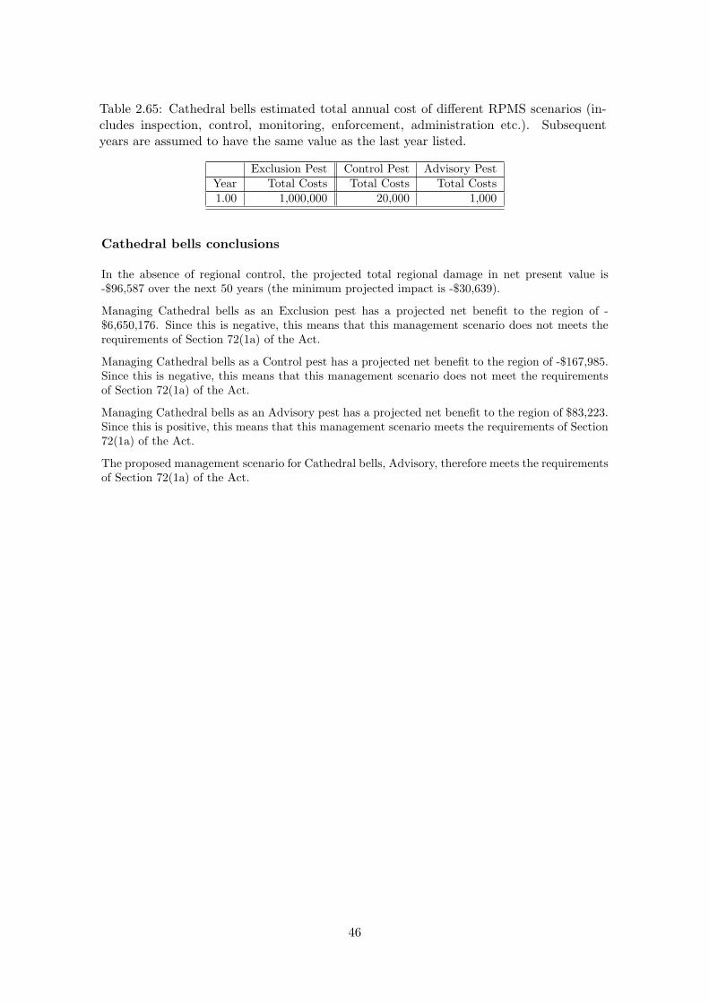
Table 2.65: Cathedral bells estimated total annual cost of di↵erent RPMS scenarios (in-cludes inspection, control, monitoring, enforcement, administration etc.). Subsequentyears are assumed to have the same value as the last year listed.
Exclusion Pest Control Pest Advisory PestYear Total Costs Total Costs Total Costs1.00 1,000,000 20,000 1,000
Cathedral bells conclusions
In the absence of regional control, the projected total regional damage in net present value is-$96,587 over the next 50 years (the minimum projected impact is -$30,639).
Managing Cathedral bells as an Exclusion pest has a projected net benefit to the region of -$6,650,176. Since this is negative, this means that this management scenario does not meets therequirements of Section 72(1a) of the Act.
Managing Cathedral bells as a Control pest has a projected net benefit to the region of -$167,985.Since this is negative, this means that this management scenario does not meet the requirementsof Section 72(1a) of the Act.
Managing Cathedral bells as an Advisory pest has a projected net benefit to the region of $83,223.Since this is positive, this means that this management scenario meets the requirements of Section72(1a) of the Act.
The proposed management scenario for Cathedral bells, Advisory, therefore meets the requirementsof Section 72(1a) of the Act.
46

0 20 40 60 80 100
0.0
0.2
0.4
0.6
0.8
1.0
Calibrated logistic growth curve, no RPMS control
Years from present
Prop
ortio
n of
max
imum
ext
ent
Current extent (ha): 10
Potential extent (ha): 98,312
(33,316−−163,308)
Time to potential (yr): 100
Current prop. of potential: <0.01
Figure 2.15: The modelled pest spread until it reaches its anticipated maximum extent.Shown are the results of the average (solid line), minimum (dotted line), and maximum(dashed line) scenarios. (A horizontal line means that the pest has already reached itsmaximum extent.) The vertical dotted-dashed lines indicate the CBA assessment periodused in this report.
47

●●
●●
●●
●●
●●
●●
●●
●●
●●
●●
●●
●●
●●
●●
●●
●●
●●
●●
●●
●●
●●
●●
●●
●
●
●
●
●
010
2030
4050
0
2000
4000
6000
8000
Popu
latio
n gr
owth
, no
RPM
S co
ntro
l
Year
s fro
m p
rese
nt
Proportion of initial area
●●
●●
●●
●●
●●
●●
●●
●●
●●
●●
●●
●●
●●
●●
●●
●●
●●
●●
●●
●●
●●
●●
●●
●●
●●
●
010
2030
4050
0
2000
4000
6000
8000
Dis
coun
ted
grow
th
Year
s fro
m p
rese
nt
Discounted annual cost
Dis
coun
t rat
e: 0
.08
Tota
l mul
tiplie
r: 12
61.4
5
(760−−
3720
)
(a)
●
●
●
●
●
●
●
●
●
●
02
46
8
0.0
0.2
0.4
0.6
0.8
1.0
Popu
latio
n gr
owth
, exc
lusi
on c
ontro
l
Year
s fro
m p
rese
ntProportion of initial area
●
●
●
●
●
●
●
●
●
●
02
46
8
0.0
0.2
0.4
0.6
0.8
1.0
Dis
coun
ted
grow
th, e
xclu
sion
con
trol
Year
s of
con
trol
Discounted annual cost
(b)
●●
●●
●●
●●
●●
●●
●●
●●
●●
●●
●●
●●
●●
●●
●●
●●
●●
●●
●●
●●
●●
●●
●●
●●
●●
●
010
2030
4050
0.0
0.2
0.4
0.6
0.8
1.0
Popu
latio
n gr
owth
, con
trol c
ontro
l
Year
s fro
m p
rese
nt
Proportion of initial area
●
●
●
●
●
●
●
●
●
●
●
●
●
●
●
●●
●●
●●
●●
●●
●●
●●
●●
●●
●●
●●
●●
●●
●●
●●
●●
●●
●●
010
2030
4050
0.0
0.2
0.4
0.6
0.8
1.0
Dis
coun
ted
grow
th, c
ontro
l con
trol
Year
s of
con
trol
Discounted annual cost
(c)
●
●
●
●
●
●
01
23
45
0.0
0.2
0.4
0.6
0.8
1.0
Popu
latio
n gr
owth
, adv
isor
y co
ntro
l
Year
s fro
m p
rese
nt
Proportion of initial area
●
●
●
●
●
●
01
23
45
0.0
0.2
0.4
0.6
0.8
1.0
Dis
coun
ted
grow
th, a
dvis
ory
cont
rol
Year
s of
con
trol
Discounted annual cost
(d)
Fig
ure
2.16
:T
hem
odel
led
popu
lati
onch
ange
sov
erth
eC
BA
asse
ssm
ent
peri
odfo
r(a
)no
regi
onal
cont
rol,
(b)
Exc
lusi
onPes
tco
ntro
l,(c
)C
ontr
olPes
tco
ntro
l,an
d(d
)A
dvis
ory
Pes
tco
ntro
l.T
heup
per
grap
hssh
owth
epo
pula
tion
chan
ges,
and
the
low
ergr
aphs
show
the
disc
ount
ing
ofas
soci
ated
impa
cts
each
year
(im
pact
sin
the
futu
rear
eof
less
valu
eec
onom
ical
lyth
anim
pact
sof
the
sam
esi
zeno
w).
48
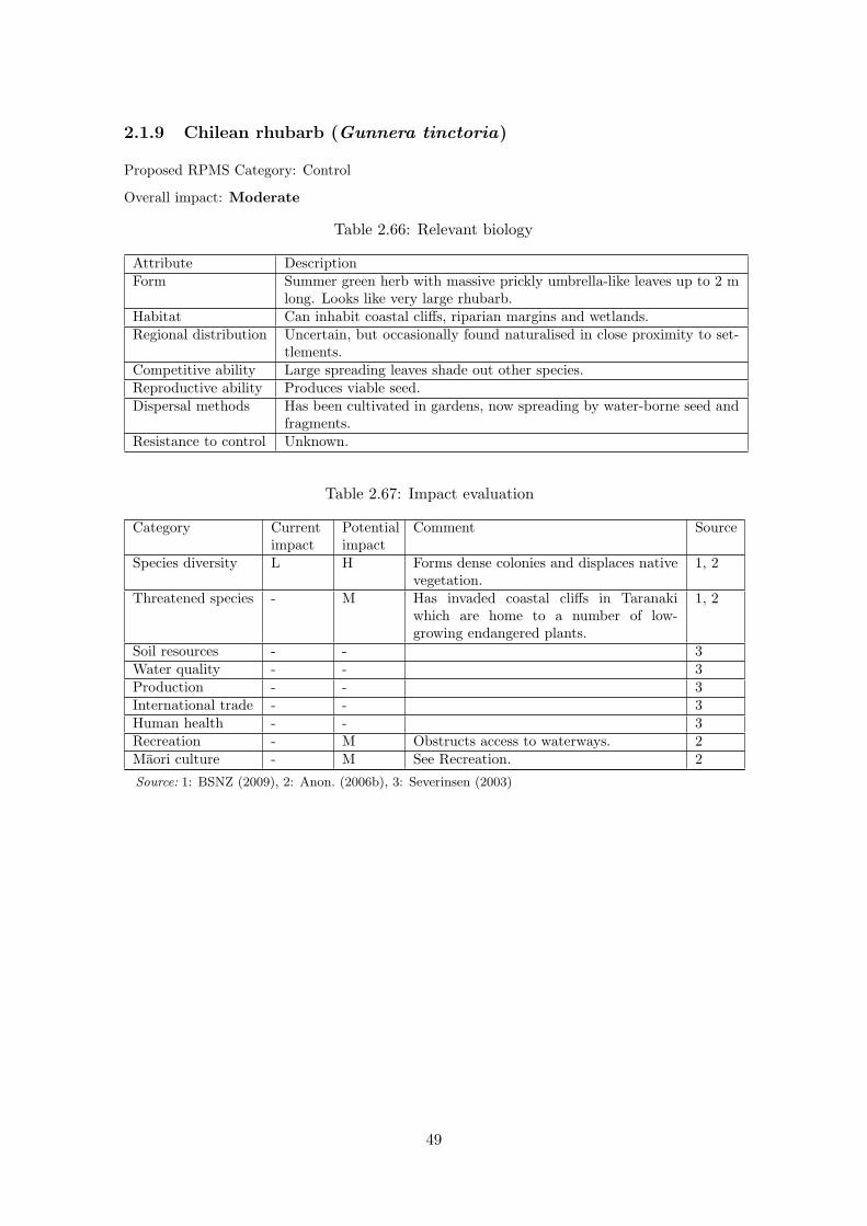
2.1.9 Chilean rhubarb (Gunnera tinctoria)
Proposed RPMS Category: Control
Overall impact: Moderate
Table 2.66: Relevant biology
Attribute DescriptionForm Summer green herb with massive prickly umbrella-like leaves up to 2 m
long. Looks like very large rhubarb.Habitat Can inhabit coastal cli↵s, riparian margins and wetlands.Regional distribution Uncertain, but occasionally found naturalised in close proximity to set-
tlements.Competitive ability Large spreading leaves shade out other species.Reproductive ability Produces viable seed.Dispersal methods Has been cultivated in gardens, now spreading by water-borne seed and
fragments.Resistance to control Unknown.
Table 2.67: Impact evaluation
Category Currentimpact
Potentialimpact
Comment Source
Species diversity L H Forms dense colonies and displaces nativevegetation.
1, 2
Threatened species - M Has invaded coastal cli↵s in Taranakiwhich are home to a number of low-growing endangered plants.
1, 2
Soil resources - - 3Water quality - - 3Production - - 3International trade - - 3Human health - - 3Recreation - M Obstructs access to waterways. 2Maori culture - M See Recreation. 2Source: 1: BSNZ (2009), 2: Anon. (2006b), 3: Severinsen (2003)
49

Chilean rhubarb CBA results
The following are results for cost-benefit analyses for four scenarios, no regional RPMS control,RPMS control as an Exclusion Pest, RPMS control as a Control Pest, and RPMS control as anAdvisory Pest. For the purposes of the CBA calculations, the pest is assumed to continue expandingwith no regional RPMS control, its spread is assumed to be near-arrested under Advisory Controlbut not reduced, and it is assumed to be successfully reduced to the expected smaller extent whenlisted as a Control Pest, more so as an Exclusion pest.
Table 2.68: Chilean rhubarb CBA results for four RPMS scenarios, presented as netpresent value (NPV, $) over 50 years. The expenditure refers to regional expenditureunder the RPMS. Minimum and maximum values are in brackets beneath average values.
Scenario Pest impacts Control benefit Expenditure Net benefitNo RPMS 250,774 0 0 -250,774
(98,762–998,333) (-98,762 – -998,333)
Exclusion Pest 2 250,772 1,686,660 -1,435,888(0–4) (98,762–998,329) (-1,587,898 – -688,331)
Control Pest 6 250,768 66,061 184,707(1–10) (98,761–998,323) (32,700 – 932,262)
Advisory Pest 3 250,771 13,212 237,559(1–4) (98,761–998,329) (85,549 – 985,117)
Table 2.69: Chilean rhubarb CBA base assumptions.
Base assumptions ValuesCurrent area infested (ha) 1
Total area potentially infested (ha) 103,808 (35,083–172,532)
Years from naturalisation to total area 75Assessment duration (yr) 50
Weighted average impact per hectare of infested land ($/ha) 0.52 (0.1–0.94)
Any benefits provided by the weed 0Discount rate 0.08
Table 2.70: Chilean rhubarb RPMS Exclusion Pest assumptions.
Exclusion Pest assumptions ValuesYears to achieve objectives 9
Final area infested (ha) 0.1 (0–0.2)
Table 2.71: Chilean rhubarb RPMS Control Pest assumptions.
Control Pest assumptions ValuesYears to achieve objectives 50
Final area infested (ha) 1 (0–1)
Table 2.72: Chilean rhubarb RPMS Advisory Pest assumptions.
Advisory Pest assumptions ValuesYears to achieve objectives 5
50

Final area infested (ha) 1 (1–2)
Table 2.73: Chilean rhubarb estimated total annual cost of di↵erent RPMS scenarios(includes inspection, control, monitoring, enforcement, administration etc.). Subsequentyears are assumed to have the same value as the last year listed.
Exclusion Pest Control Pest Advisory PestYear Total Costs Total Costs Total Costs1.00 250,000 5,000 1,000
Chilean rhubarb conclusions
In the absence of regional control, the projected total regional damage in net present value is-$250,774 over the next 50 years (the minimum projected impact is -$98,762).
Managing Chilean rhubarb as an Exclusion pest has a projected net benefit to the region of -$1,435,888. Since this is negative, this means that this management scenario does not meets therequirements of Section 72(1a) of the Act.
Managing Chilean rhubarb as a Control pest has a projected net benefit to the region of $184,707.Since this is positive, this means that this management scenario meets the requirements of Section72(1a) of the Act.
Managing Chilean rhubarb as an Advisory pest has a projected net benefit to the region of $237,559.Since this is positive, this means that this management scenario meets the requirements of Section72(1a) of the Act.
The proposed management scenario for Chilean rhubarb, Control, therefore meets the requirementsof Section 72(1a) of the Act.
51

0 20 40 60
0.0
0.2
0.4
0.6
0.8
1.0
Calibrated logistic growth curve, no RPMS control
Years from present
Prop
ortio
n of
max
imum
ext
ent
Current extent (ha): 1
Potential extent (ha): 103,808
(35,083−−172,532)
Time to potential (yr): 75
Current prop. of potential: <0.01
Figure 2.17: The modelled pest spread until it reaches its anticipated maximum extent.Shown are the results of the average (solid line), minimum (dotted line), and maximum(dashed line) scenarios. (A horizontal line means that the pest has already reached itsmaximum extent.) The vertical dotted-dashed lines indicate the CBA assessment periodused in this report.
52

●●
●●
●●
●●
●●
●●
●●
●●
●●
●●
●●
●●
●●
●●
●●
●●
●●
●●
●●
●●
●●
●●
●●
●●
●●
●
010
2030
4050
0
5000
0
1000
00
1500
00
Popu
latio
n gr
owth
, no
RPM
S co
ntro
l
Year
s fro
m p
rese
nt
Proportion of initial area
●●
●●
●●
●●
●●
●●
●●
●●
●●
●●
●●
●●
●●
●●
●●
●●
●●
●●
●●
●●
●●
●●
●●
●●
●●
●
010
2030
4050
0
5000
0
1000
00
1500
00
Dis
coun
ted
grow
th
Year
s fro
m p
rese
nt
Discounted annual cost
Dis
coun
t rat
e: 0
.08
Tota
l mul
tiplie
r: 39
134.
14
(235
46−−
1157
91)
(a)
●
●
●
●
●
●
●
●
●
●
02
46
8
0.0
0.2
0.4
0.6
0.8
1.0
Popu
latio
n gr
owth
, exc
lusi
on c
ontro
l
Year
s fro
m p
rese
ntProportion of initial area
●
●
●
●
●
●
●
●
●
●
02
46
8
0.0
0.2
0.4
0.6
0.8
1.0
Dis
coun
ted
grow
th, e
xclu
sion
con
trol
Year
s of
con
trol
Discounted annual cost
(b)
●●
●●
●●
●●
●●
●●
●●
●●
●●
●●
●●
●●
●●
●●
●●
●●
●●
●●
●●
●●
●●
●●
●●
●●
●●
●
010
2030
4050
0.0
0.2
0.4
0.6
0.8
1.0
Popu
latio
n gr
owth
, con
trol c
ontro
l
Year
s fro
m p
rese
nt
Proportion of initial area
●
●
●
●
●
●
●
●
●
●
●
●
●
●
●
●●
●●
●●
●●
●●
●●
●●
●●
●●
●●
●●
●●
●●
●●
●●
●●
●●
●●
010
2030
4050
0.0
0.2
0.4
0.6
0.8
1.0
Dis
coun
ted
grow
th, c
ontro
l con
trol
Year
s of
con
trol
Discounted annual cost
(c)
●
●
●
●
●
●
01
23
45
0.0
0.2
0.4
0.6
0.8
1.0
Popu
latio
n gr
owth
, adv
isor
y co
ntro
l
Year
s fro
m p
rese
nt
Proportion of initial area
●
●
●
●
●
●
01
23
45
0.0
0.2
0.4
0.6
0.8
1.0
Dis
coun
ted
grow
th, a
dvis
ory
cont
rol
Year
s of
con
trol
Discounted annual cost
(d)
Fig
ure
2.18
:T
hem
odel
led
popu
lati
onch
ange
sov
erth
eC
BA
asse
ssm
ent
peri
odfo
r(a
)no
regi
onal
cont
rol,
(b)
Exc
lusi
onPes
tco
ntro
l,(c
)C
ontr
olPes
tco
ntro
l,an
d(d
)A
dvis
ory
Pes
tco
ntro
l.T
heup
per
grap
hssh
owth
epo
pula
tion
chan
ges,
and
the
low
ergr
aphs
show
the
disc
ount
ing
ofas
soci
ated
impa
cts
each
year
(im
pact
sin
the
futu
rear
eof
less
valu
eec
onom
ical
lyth
anim
pact
sof
the
sam
esi
zeno
w).
53

2.1.10 Climbing spindleberry (Celastrus orbiculatus)
Proposed RPMS Category: Control
Overall impact: Major
Table 2.74: Relevant biology
Attribute DescriptionForm A deciduous climber that can grow to 12 m high. Produces yellow fruit,
which open to expose a scarlet centre.Habitat Forest margins, scrub and gardens.Regional distribution Rotorua area, isolated sites in other parts of the region.Competitive ability Can smother and out-compete native species.Reproductive ability Produces viable seed.Dispersal methods Has been planted in some areas as an ornamental, its seeds are also
dispersed by birds.Resistance to control Can be controlled using foliar or stump application of herbicide.
Table 2.75: Impact evaluation
Category Currentimpact
Potentialimpact
Comment Source
Species diversity M H Stems strangle host, overtop mostcanopies and cause collapse.
1, 2
Threatened species - H 1, 2Soil resources - - 3Water quality - - 3Production L M Smothers trees in plantation forests, cre-
ates safety hazard during harvest of plan-tation trees. Can damage shelterbelts.
2, 4
International trade - - 3Human health - - 3Recreation L M Layering stems become dense and obstruct
access to forest.1, 2
Maori culture L M See Recreation. 1Source: 1: Craw (2000), 2: Anon. (2004a), 3: Severinsen (2003), 4: Stahl (2009)
54
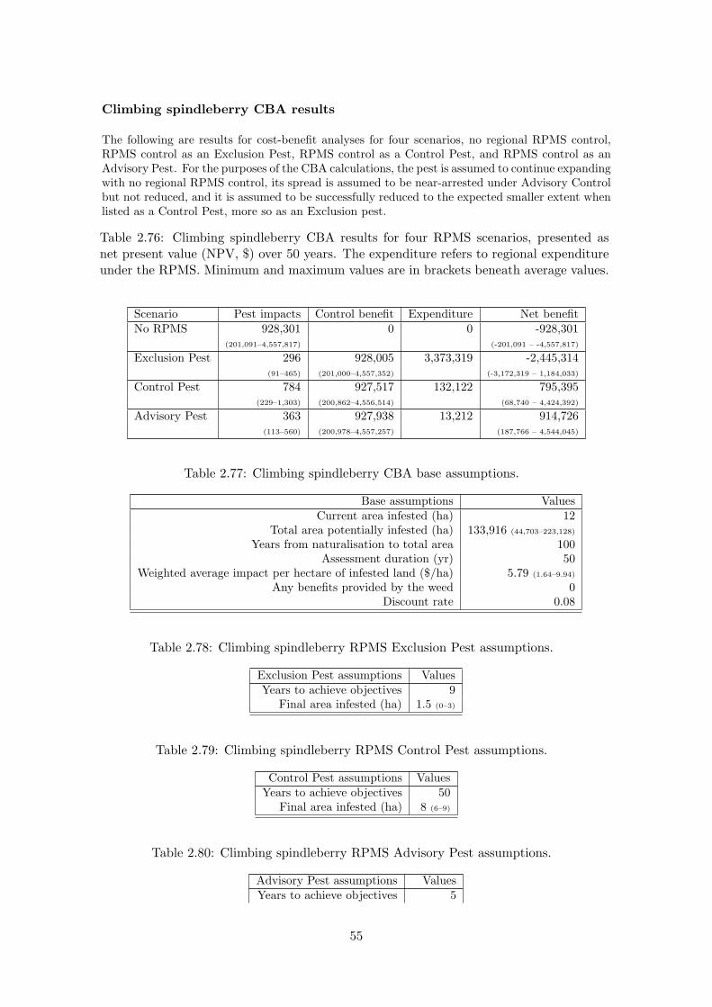
Climbing spindleberry CBA results
The following are results for cost-benefit analyses for four scenarios, no regional RPMS control,RPMS control as an Exclusion Pest, RPMS control as a Control Pest, and RPMS control as anAdvisory Pest. For the purposes of the CBA calculations, the pest is assumed to continue expandingwith no regional RPMS control, its spread is assumed to be near-arrested under Advisory Controlbut not reduced, and it is assumed to be successfully reduced to the expected smaller extent whenlisted as a Control Pest, more so as an Exclusion pest.
Table 2.76: Climbing spindleberry CBA results for four RPMS scenarios, presented asnet present value (NPV, $) over 50 years. The expenditure refers to regional expenditureunder the RPMS. Minimum and maximum values are in brackets beneath average values.
Scenario Pest impacts Control benefit Expenditure Net benefitNo RPMS 928,301 0 0 -928,301
(201,091–4,557,817) (-201,091 – -4,557,817)
Exclusion Pest 296 928,005 3,373,319 -2,445,314(91–465) (201,000–4,557,352) (-3,172,319 – 1,184,033)
Control Pest 784 927,517 132,122 795,395(229–1,303) (200,862–4,556,514) (68,740 – 4,424,392)
Advisory Pest 363 927,938 13,212 914,726(113–560) (200,978–4,557,257) (187,766 – 4,544,045)
Table 2.77: Climbing spindleberry CBA base assumptions.
Base assumptions ValuesCurrent area infested (ha) 12
Total area potentially infested (ha) 133,916 (44,703–223,128)
Years from naturalisation to total area 100Assessment duration (yr) 50
Weighted average impact per hectare of infested land ($/ha) 5.79 (1.64–9.94)
Any benefits provided by the weed 0Discount rate 0.08
Table 2.78: Climbing spindleberry RPMS Exclusion Pest assumptions.
Exclusion Pest assumptions ValuesYears to achieve objectives 9
Final area infested (ha) 1.5 (0–3)
Table 2.79: Climbing spindleberry RPMS Control Pest assumptions.
Control Pest assumptions ValuesYears to achieve objectives 50
Final area infested (ha) 8 (6–9)
Table 2.80: Climbing spindleberry RPMS Advisory Pest assumptions.
Advisory Pest assumptions ValuesYears to achieve objectives 5
55

Final area infested (ha) 15 (12–18)
Table 2.81: Climbing spindleberry estimated total annual cost of di↵erent RPMS scenarios(includes inspection, control, monitoring, enforcement, administration etc.). Subsequentyears are assumed to have the same value as the last year listed.
Exclusion Pest Control Pest Advisory PestYear Total Costs Total Costs Total Costs1.00 500,000 10,000 1,000
Climbing spindleberry conclusions
In the absence of regional control, the projected total regional damage in net present value is-$928,301 over the next 50 years (the minimum projected impact is -$201,091).
Managing Climbing spindleberry as an Exclusion pest has a projected net benefit to the region of-$2,445,314. Since this is negative, this means that this management scenario does not meets therequirements of Section 72(1a) of the Act.
Managing Climbing spindleberry as a Control pest has a projected net benefit to the region of$795,395. Since this is positive, this means that this management scenario meets the requirementsof Section 72(1a) of the Act.
Managing Climbing spindleberry as an Advisory pest has a projected net benefit to the region of$914,726. Since this is positive, this means that this management scenario meets the requirementsof Section 72(1a) of the Act.
The proposed management scenario for Climbing spindleberry, Control, therefore meets the re-quirements of Section 72(1a) of the Act.
56

0 20 40 60 80 100
0.0
0.2
0.4
0.6
0.8
1.0
Calibrated logistic growth curve, no RPMS control
Years from present
Prop
ortio
n of
max
imum
ext
ent
Current extent (ha): 12
Potential extent (ha): 133,916
(44,703−−223,128)
Time to potential (yr): 100
Current prop. of potential: <0.01
Figure 2.19: The modelled pest spread until it reaches its anticipated maximum extent.Shown are the results of the average (solid line), minimum (dotted line), and maximum(dashed line) scenarios. (A horizontal line means that the pest has already reached itsmaximum extent.) The vertical dotted-dashed lines indicate the CBA assessment periodused in this report.
57

●●
●●
●●
●●
●●
●●
●●
●●
●●
●●
●●
●●
●●
●●
●●
●●
●●
●●
●●
●●
●●
●●
●●
●
●
●
●
●
010
2030
4050
0
2000
4000
6000
8000
Popu
latio
n gr
owth
, no
RPM
S co
ntro
l
Year
s fro
m p
rese
nt
Proportion of initial area
●●
●●
●●
●●
●●
●●
●●
●●
●●
●●
●●
●●
●●
●●
●●
●●
●●
●●
●●
●●
●●
●●
●●
●●
●●
●
010
2030
4050
0
2000
4000
6000
8000
Dis
coun
ted
grow
th
Year
s fro
m p
rese
nt
Discounted annual cost
Dis
coun
t rat
e: 0
.08
Tota
l mul
tiplie
r: 14
14.6
8
(849−−
4236
)
(a)
●
●
●
●
●
●
●
●
●
●
02
46
8
0.0
0.2
0.4
0.6
0.8
1.0
Popu
latio
n gr
owth
, exc
lusi
on c
ontro
l
Year
s fro
m p
rese
ntProportion of initial area
●
●
●
●
●
●
●
●
●
●
02
46
8
0.0
0.2
0.4
0.6
0.8
1.0
Dis
coun
ted
grow
th, e
xclu
sion
con
trol
Year
s of
con
trol
Discounted annual cost
(b)
●●
●●
●●
●●
●●
●●
●●
●●
●●
●●
●●
●●
●●
●●
●●
●●
●●
●●
●●
●●
●●
●●
●●
●●
●●
●
010
2030
4050
0.0
0.2
0.4
0.6
0.8
1.0
Popu
latio
n gr
owth
, con
trol c
ontro
l
Year
s fro
m p
rese
nt
Proportion of initial area
●
●
●
●
●
●
●
●
●
●
●
●
●
●
●
●●
●●
●●
●●
●●
●●
●●
●●
●●
●●
●●
●●
●●
●●
●●
●●
●●
●●
010
2030
4050
0.0
0.2
0.4
0.6
0.8
1.0
Dis
coun
ted
grow
th, c
ontro
l con
trol
Year
s of
con
trol
Discounted annual cost
(c)
●
●
●
●
●
●
01
23
45
0.0
0.2
0.4
0.6
0.8
1.0
Popu
latio
n gr
owth
, adv
isor
y co
ntro
l
Year
s fro
m p
rese
nt
Proportion of initial area
●
●
●
●
●
●
01
23
45
0.0
0.2
0.4
0.6
0.8
1.0
Dis
coun
ted
grow
th, a
dvis
ory
cont
rol
Year
s of
con
trol
Discounted annual cost
(d)
Fig
ure
2.20
:T
hem
odel
led
popu
lati
onch
ange
sov
erth
eC
BA
asse
ssm
ent
peri
odfo
r(a
)no
regi
onal
cont
rol,
(b)
Exc
lusi
onPes
tco
ntro
l,(c
)C
ontr
olPes
tco
ntro
l,an
d(d
)A
dvis
ory
Pes
tco
ntro
l.T
heup
per
grap
hssh
owth
epo
pula
tion
chan
ges,
and
the
low
ergr
aphs
show
the
disc
ount
ing
ofas
soci
ated
impa
cts
each
year
(im
pact
sin
the
futu
rear
eof
less
valu
eec
onom
ical
lyth
anim
pact
sof
the
sam
esi
zeno
w).
58

2.1.11 Coast tea tree (Leptospermum laevigatum)
Proposed RPMS Category: Control
Overall impact: Major
Table 2.82: Relevant biology
Attribute DescriptionForm Tall, bushy shrub or small, twisted tree, to 6 m. Leaves are grey-green,
obovate, to 2 cm. Flowers are white, to 1.5 cm diameter, in spring orearly summer.
Habitat Coastal sand dunes, shrubland.Regional distribution Matakana Island.Competitive ability Highly tolerant of salt spray.Reproductive ability Woody capsules shed large numbers of seeds.Dispersal methods Gravity, wind. Deliberately planted for sand stabilisation.Resistance to control Unknown.Benefits Minor benefit to production (forestry) as it bu↵ers a pine plantation
from salt spray on Matakana Island.
Table 2.83: Impact evaluation
Category Currentimpact
Potentialimpact
Comment Source
Species diversity H H Excludes native sand-binders (pingao andspinifex), alters sand-dune community.
1, 2, 3
Threatened species M H Displaces Pimelia arenaria in sand dunes. 3, 4Soil resources L H Exacerbates fore dune erosion, as it ex-
cludes native sand-binders and its rootsdo not bind sand..
3
Water quality - - 3Production - - 5International trade - - 6Human health - - 6Recreation L M Blocks access to beaches and sand dunes. 3Maori culture L M See Recreation. 3Source: 1: Williams et al. (2005), 2: Hicks et al. (2001), 3: Stahl (2009), 4: de Lange et al. (2009), 5:
Anon. (2010c), 6: Severinsen (2003)
59

Coast tea tree CBA results
The following are results for cost-benefit analyses for four scenarios, no regional RPMS control,RPMS control as an Exclusion Pest, RPMS control as a Control Pest, and RPMS control as anAdvisory Pest. For the purposes of the CBA calculations, the pest is assumed to continue expandingwith no regional RPMS control, its spread is assumed to be near-arrested under Advisory Controlbut not reduced, and it is assumed to be successfully reduced to the expected smaller extent whenlisted as a Control Pest, more so as an Exclusion pest.
Table 2.84: Coast tea tree CBA results for four RPMS scenarios, presented as net presentvalue (NPV, $) over 50 years. The expenditure refers to regional expenditure under theRPMS. Minimum and maximum values are in brackets beneath average values.
Scenario Pest impacts Control benefit Expenditure Net benefitNo RPMS 702,429 0 0 -702,429
(302,844–2,784,693) (-302,844 – -2,784,693)
Exclusion Pest 885 701,544 674,664 26,880(633–1,087) (302,211–2,783,606) (-372,453 – 2,108,942)
Control Pest 2,344 700,085 26,424 673,661(1,593–3,045) (301,251–2,781,648) (274,827 – 2,755,224)
Advisory Pest 1,086 701,343 13,212 688,131(788–1,310) (302,056–2,783,383) (288,844 – 2,770,171)
Table 2.85: Coast tea tree CBA base assumptions.
Base assumptions ValuesCurrent area infested (ha) 30
Total area potentially infested (ha) 97,434 (32,954–161,915)
Years from naturalisation to total area 50Assessment duration (yr) 50
Weighted average impact per hectare of infested land ($/ha) 6.93 (4.57–9.29)
Any benefits provided by the weed 1Discount rate 0.08
Table 2.86: Coast tea tree RPMS Exclusion Pest assumptions.
Exclusion Pest assumptions ValuesYears to achieve objectives 9
Final area infested (ha) 3.8 (0–7.5)
Table 2.87: Coast tea tree RPMS Control Pest assumptions.
Control Pest assumptions ValuesYears to achieve objectives 50
Final area infested (ha) 19 (15–22)
Table 2.88: Coast tea tree RPMS Advisory Pest assumptions.
Advisory Pest assumptions ValuesYears to achieve objectives 5
Final area infested (ha) 38 (30–45)
60

Table 2.89: Coast tea tree estimated total annual cost of di↵erent RPMS scenarios (in-cludes inspection, control, monitoring, enforcement, administration etc.). Subsequentyears are assumed to have the same value as the last year listed.
Exclusion Pest Control Pest Advisory PestYear Total Costs Total Costs Total Costs1.00 100,000 2,000 1,000
Coast tea tree conclusions
In the absence of regional control, the projected total regional damage in net present value is-$702,429 over the next 50 years (the minimum projected impact is -$302,844).
Managing Coast tea tree as an Exclusion pest has a projected net benefit to the region of $26,880.Since this is positive, this means that this management scenario meets the requirements of Section72(1a) of the Act.
Managing Coast tea tree as a Control pest has a projected net benefit to the region of $673,661.Since this is positive, this means that this management scenario meets the requirements of Section72(1a) of the Act.
Managing Coast tea tree as an Advisory pest has a projected net benefit to the region of $688,131.Since this is positive, this means that this management scenario meets the requirements of Section72(1a) of the Act.
The proposed management scenario for Coast tea tree, Control, therefore meets the requirementsof Section 72(1a) of the Act.
61

0 10 20 30 40 50
0.0
0.2
0.4
0.6
0.8
1.0
Calibrated logistic growth curve, no RPMS control
Years from present
Prop
ortio
n of
max
imum
ext
ent
Current extent (ha): 30
Potential extent (ha): 97,434
(32,954−−161,915)
Time to potential (yr): 50
Current prop. of potential: 0.001
Figure 2.21: The modelled pest spread until it reaches its anticipated maximum extent.Shown are the results of the average (solid line), minimum (dotted line), and maximum(dashed line) scenarios. (A horizontal line means that the pest has already reached itsmaximum extent.) The vertical dotted-dashed lines indicate the CBA assessment periodused in this report.
62

●●
●●
●●
●●
●●
●●
●●
●●
●●
●●
●●
●
●
●
●
●
●
●●
●●
●●
●●
●●
●●
●●
●●
●●
●●
●●
●
010
2030
4050
0
1000
2000
3000
4000
5000
Popu
latio
n gr
owth
, no
RPM
S co
ntro
l
Year
s fro
m p
rese
nt
Proportion of initial area
●●
●●
●●
●●
●●
●●
●●
●●
●●
●●
●●
●●
●●
●●
●●
●●
●●
●●
●●
●●
●●
●●
●●
●●
●●
●
010
2030
4050
0
1000
2000
3000
4000
5000
Dis
coun
ted
grow
th
Year
s fro
m p
rese
nt
Discounted annual cost
Dis
coun
t rat
e: 0
.08
Tota
l mul
tiplie
r: 33
78.2
5
(221
0−−9
986)
(a)
●
●
●
●
●
●
●
●
●
●
02
46
8
0.0
0.2
0.4
0.6
0.8
1.0
Popu
latio
n gr
owth
, exc
lusi
on c
ontro
l
Year
s fro
m p
rese
ntProportion of initial area
●
●
●
●
●
●
●
●
●
●
02
46
8
0.0
0.2
0.4
0.6
0.8
1.0
Dis
coun
ted
grow
th, e
xclu
sion
con
trol
Year
s of
con
trol
Discounted annual cost
(b)
●●
●●
●●
●●
●●
●●
●●
●●
●●
●●
●●
●●
●●
●●
●●
●●
●●
●●
●●
●●
●●
●●
●●
●●
●●
●
010
2030
4050
0.0
0.2
0.4
0.6
0.8
1.0
Popu
latio
n gr
owth
, con
trol c
ontro
l
Year
s fro
m p
rese
nt
Proportion of initial area
●
●
●
●
●
●
●
●
●
●
●
●
●
●
●
●●
●●
●●
●●
●●
●●
●●
●●
●●
●●
●●
●●
●●
●●
●●
●●
●●
●●
010
2030
4050
0.0
0.2
0.4
0.6
0.8
1.0
Dis
coun
ted
grow
th, c
ontro
l con
trol
Year
s of
con
trol
Discounted annual cost
(c)
●
●
●
●
●
●
01
23
45
0.0
0.2
0.4
0.6
0.8
1.0
Popu
latio
n gr
owth
, adv
isor
y co
ntro
l
Year
s fro
m p
rese
nt
Proportion of initial area
●
●
●
●
●
●
01
23
45
0.0
0.2
0.4
0.6
0.8
1.0
Dis
coun
ted
grow
th, a
dvis
ory
cont
rol
Year
s of
con
trol
Discounted annual cost
(d)
Fig
ure
2.22
:T
hem
odel
led
popu
lati
onch
ange
sov
erth
eC
BA
asse
ssm
ent
peri
odfo
r(a
)no
regi
onal
cont
rol,
(b)
Exc
lusi
onPes
tco
ntro
l,(c
)C
ontr
olPes
tco
ntro
l,an
d(d
)A
dvis
ory
Pes
tco
ntro
l.T
heup
per
grap
hssh
owth
epo
pula
tion
chan
ges,
and
the
low
ergr
aphs
show
the
disc
ount
ing
ofas
soci
ated
impa
cts
each
year
(im
pact
sin
the
futu
rear
eof
less
valu
eec
onom
ical
lyth
anim
pact
sof
the
sam
esi
zeno
w).
63

2.1.12 Darwin’s barberry (Berberis darwinii)
Proposed RPMS Category: Control
Overall impact: Moderate
Table 2.90: Relevant biology
Attribute DescriptionForm Evergreen shrub up to 4 m tall with holly-like leaves and purple berries.Habitat Shade tolerant, can survive in a variety of habitats.Regional distribution South of Rotorua, otherwise extent unknown.Competitive ability Can form impenetrable stands. May invade forest as it is shade tolerant.Reproductive ability Produces viable seed.Dispersal methods Has been planted as a hedge plant in some areas; birds also disperse the
seed.Resistance to control Unknown.
Table 2.91: Impact evaluation
Category Currentimpact
Potentialimpact
Comment Source
Species diversity L M Can invade forest as it is shade-tolerant,forms impenetrable thickets and out-competes native forest and shrublandspecies.
1
Threatened species - M 1Soil resources - - 2Water quality - - 2Production L L Excludes pasture species. Nuisance in
plantation forestry.1, 3, 4
International trade - - 2Human health - - 2Recreation - L Prickly spines restrict access. 1Maori culture - M Obstructs access to cultural sites (e.g.
waahi tapu, urupa).2
Source: 1: Anon. (2006a), 2: Severinsen (2003), 3: Craw (2000), 4: Mallinson (2009)
64

Darwin’s barberry CBA results
The following are results for cost-benefit analyses for four scenarios, no regional RPMS control,RPMS control as an Exclusion Pest, RPMS control as a Control Pest, and RPMS control as anAdvisory Pest. For the purposes of the CBA calculations, the pest is assumed to continue expandingwith no regional RPMS control, its spread is assumed to be near-arrested under Advisory Controlbut not reduced, and it is assumed to be successfully reduced to the expected smaller extent whenlisted as a Control Pest, more so as an Exclusion pest.
Table 2.92: Darwin’s barberry CBA results for four RPMS scenarios, presented as netpresent value (NPV, $) over 50 years. The expenditure refers to regional expenditureunder the RPMS. Minimum and maximum values are in brackets beneath average values.
Scenario Pest impacts Control benefit Expenditure Net benefitNo RPMS 347,282 0 0 -347,282
(62,999–974,067) (-62,999 – -974,067)
Exclusion Pest 14,905 332,377 1,011,996 -679,619(3,234–24,556) (59,765–949,511) (-952,231 – -62,485)
Control Pest 39,455 307,827 39,636 268,191(8,137–68,805) (54,862–905,262) (15,226 – 865,626)
Advisory Pest 18,281 329,001 13,212 315,789(4,024–29,591) (58,975–944,476) (45,763 – 931,264)
Table 2.93: Darwin’s barberry CBA base assumptions.
Base assumptions ValuesCurrent area infested (ha) 100
Total area potentially infested (ha) 141,607 (47,641–235,573)
Years from naturalisation to total area 125Assessment duration (yr) 50
Weighted average impact per hectare of infested land ($/ha) 35 (7–63)
Any benefits provided by the weed 0Discount rate 0.08
Table 2.94: Darwin’s barberry RPMS Exclusion Pest assumptions.
Exclusion Pest assumptions ValuesYears to achieve objectives 9
Final area infested (ha) 12.5 (0–25)
Table 2.95: Darwin’s barberry RPMS Control Pest assumptions.
Control Pest assumptions ValuesYears to achieve objectives 50
Final area infested (ha) 62 (50–75)
Table 2.96: Darwin’s barberry RPMS Advisory Pest assumptions.
Advisory Pest assumptions ValuesYears to achieve objectives 5
65

Final area infested (ha) 125 (100–150)
Table 2.97: Darwin’s barberry estimated total annual cost of di↵erent RPMS scenarios(includes inspection, control, monitoring, enforcement, administration etc.). Subsequentyears are assumed to have the same value as the last year listed.
Exclusion Pest Control Pest Advisory PestYear Total Costs Total Costs Total Costs1.00 150,000 3,000 1,000
Darwin’s barberry conclusions
In the absence of regional control, the projected total regional damage in net present value is-$347,282 over the next 50 years (the minimum projected impact is -$62,999).
Managing Darwin’s barberry as an Exclusion pest has a projected net benefit to the region of-$679,619. Since this is negative, this means that this management scenario does not meets therequirements of Section 72(1a) of the Act.
Managing Darwin’s barberry as a Control pest has a projected net benefit to the region of $268,191.Since this is positive, this means that this management scenario meets the requirements of Section72(1a) of the Act.
Managing Darwin’s barberry as an Advisory pest has a projected net benefit to the region of$315,789. Since this is positive, this means that this management scenario meets the requirementsof Section 72(1a) of the Act.
The proposed management scenario for Darwin’s barberry, Control, therefore meets the require-ments of Section 72(1a) of the Act.
66

0 20 40 60 80 100 120
0.0
0.2
0.4
0.6
0.8
1.0
Calibrated logistic growth curve, no RPMS control
Years from present
Prop
ortio
n of
max
imum
ext
ent
Current extent (ha): 100
Potential extent (ha): 141,607
(47,641−−235,573)
Time to potential (yr): 125
Current prop. of potential: 0.001
Figure 2.23: The modelled pest spread until it reaches its anticipated maximum extent.Shown are the results of the average (solid line), minimum (dotted line), and maximum(dashed line) scenarios. (A horizontal line means that the pest has already reached itsmaximum extent.) The vertical dotted-dashed lines indicate the CBA assessment periodused in this report.
67
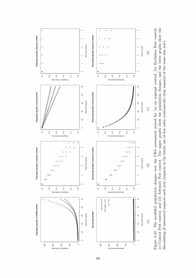
●●
●●
●●
●●
●●
●●
●●
●●
●●
●●
●●
●●
●●
●●
●●
●●
●●
●●
●●
●●
●●
●
●
●
●
●
●
●
●
●
010
2030
4050
0
100
200
300
400
Popu
latio
n gr
owth
, no
RPM
S co
ntro
l
Year
s fro
m p
rese
nt
Proportion of initial area
●●
●●
●●
●●
●●
●●
●●
●●
●●
●●
●●
●●
●●
●●
●●
●●
●●
●●
●●
●●
●●
●●
●●
●●
●●
●
010
2030
4050
0
100
200
300
400
Dis
coun
ted
grow
th
Year
s fro
m p
rese
nt
Discounted annual cost
Dis
coun
t rat
e: 0
.08
Tota
l mul
tiplie
r: 13
2.57
(113−−
221)
(a)
●
●
●
●
●
●
●
●
●
●
02
46
8
0.0
0.2
0.4
0.6
0.8
1.0
Popu
latio
n gr
owth
, exc
lusi
on c
ontro
l
Year
s fro
m p
rese
ntProportion of initial area
●
●
●
●
●
●
●
●
●
●
02
46
8
0.0
0.2
0.4
0.6
0.8
1.0
Dis
coun
ted
grow
th, e
xclu
sion
con
trol
Year
s of
con
trol
Discounted annual cost
(b)
●●
●●
●●
●●
●●
●●
●●
●●
●●
●●
●●
●●
●●
●●
●●
●●
●●
●●
●●
●●
●●
●●
●●
●●
●●
●
010
2030
4050
0.0
0.2
0.4
0.6
0.8
1.0
Popu
latio
n gr
owth
, con
trol c
ontro
l
Year
s fro
m p
rese
nt
Proportion of initial area
●
●
●
●
●
●
●
●
●
●
●
●
●
●
●
●●
●●
●●
●●
●●
●●
●●
●●
●●
●●
●●
●●
●●
●●
●●
●●
●●
●●
010
2030
4050
0.0
0.2
0.4
0.6
0.8
1.0
Dis
coun
ted
grow
th, c
ontro
l con
trol
Year
s of
con
trol
Discounted annual cost
(c)
●
●
●
●
●
●
01
23
45
0.0
0.2
0.4
0.6
0.8
1.0
Popu
latio
n gr
owth
, adv
isor
y co
ntro
l
Year
s fro
m p
rese
nt
Proportion of initial area
●
●
●
●
●
●
01
23
45
0.0
0.2
0.4
0.6
0.8
1.0
Dis
coun
ted
grow
th, a
dvis
ory
cont
rol
Year
s of
con
trol
Discounted annual cost
(d)
Fig
ure
2.24
:T
hem
odel
led
popu
lati
onch
ange
sov
erth
eC
BA
asse
ssm
ent
peri
odfo
r(a
)no
regi
onal
cont
rol,
(b)
Exc
lusi
onPes
tco
ntro
l,(c
)C
ontr
olPes
tco
ntro
l,an
d(d
)A
dvis
ory
Pes
tco
ntro
l.T
heup
per
grap
hssh
owth
epo
pula
tion
chan
ges,
and
the
low
ergr
aphs
show
the
disc
ount
ing
ofas
soci
ated
impa
cts
each
year
(im
pact
sin
the
futu
rear
eof
less
valu
eec
onom
ical
lyth
anim
pact
sof
the
sam
esi
zeno
w).
68

2.1.13 Egeria densa (Egeria densa)
Proposed RPMS Category: Control (defined lakes)
Overall impact: Major
Table 2.98: Relevant biology
Attribute DescriptionForm Submerged, bottom-rooting perennial, growing to 5 m. Stems slender,
brittle, much-branched, buoyant, 3 mm diam. Leaves in whorls of 4-6(occ. 3 near base), linear, 15-30 x 4 mm, dark green. Flowers on surface,3 petalled, 20 mm diam, white with 9 yellow stamens, Nov-Jan.
Habitat Rivers, lakes, dunelakes, other waterbodies with mod-high light and 10-25 degrees C.
Regional distribution Lakes Okareka, Rerewhakaaitu, Rotoiti, Rotorua, Tarawera and manyother waterbodies.
Competitive abilityReproductive ability Grows easily from broken fragments. Only male plants found in NZ, no
seed set.Dispersal methods Water, humans.Resistance to control Di�cult to control.
Table 2.99: Impact evaluation
Category Currentimpact
Potentialimpact
Comment Source
Species diversity M H Forms vast underwater meadows in fresh-water up to 5 m tall, shades outsmaller native species, prevents recruit-ment. Rotting vegetation deoxygenateswater, killing fauna and flora.
1, 2, 3
Threatened species L H 1, 2Soil resources - -Water quality M H Large clumps dislodge, causing blockage
and flooding. Rotting vegetation degradeswater quality. Causes nutrient releasefrom sediments, exacerbates eutrophica-tion.
1, 3
Production - - 1, 4International trade - -Human health - L Large weed beds may support more snails
which host the waterborne schistosomecercariae larvae that cause ’swimmersitch’.
5
Recreation M H Dense masses block up lakes and shadewater, reducing access to lakes. Inconve-nience caused by biosecurity measures i.e.restricted access to lakes by lake cordons,cleaning and washing procedures.
1, 2, 3
Maori culture M H See Recreation. 1, 2, 3Source: 1: Craw (2000), 2: Roy et al. (2004), 3: Clayton & Champion (2003), 4: Department of Conser-
vation (2007), 5: NIWA (2002)
69

Egeria densa CBA results
Since Egeria densa is currently absent from the defined area, it is di�cult to accurately quantifythe costs and benefits of current and proposed e↵orts to continue to exclude the species. If thespecies were to invade this year and spread in the defined area, without regional control for thenext 50 years, the total pest impacts over this period in net present value are calculated to be$412,940 ($539,742–$442,649). This can be compared with the calculated net present value of theproposed annual expenditure on control over this same period of $408,811 (to exclude the Controlpest from the defined areas). Note that this comparison does not take into account whether or notthe proposed level of expenditure is adequate to have a high probability of excluding the speciesover this period. Given the broad experience of the biosecurity sta↵ at Environment Bay of Plenty,we assume that it will be.
The following tables provide the parameters used in this cost-benefit analysis.
Table 2.100: Egeria densa CBA base assumptions.
Base assumptions ValuesCurrent area infested (ha) 0
Total area potentially infested (ha) 432 (432–432)
Years from naturalisation to total area 25Assessment duration (yr) 50
Weighted average impact per hectare of infested land ($/ha) 7.38 (2.5–12.25)
Any benefits provided by the weed 0Discount rate 0.08
Table 2.101: Egeria densa estimated total annual cost of the proposed RPMS scenario(includes inspection, control, monitoring, enforcement, administration etc.). Subsequentyears are assumed to have the same value as the last year listed.
Exclusion PestYear Total Costs1.00 30,942
Egeria densa conclusions
Since the calculated average impact should the species establish in the defined area is greater thanthe anticipated expenditure, and establishment is likely in the absence of regional surveillance andcontrol, this management scenario meets the requirements of Section 72(1a) of the Act.
70

2.1.14 Elodea canadensis (Elodea canadensis)
Proposed RPMS Category: Advisory
Overall impact: Major
Table 2.102: Relevant biology
Attribute DescriptionForm Submerged, bottom-rooting perennial, growing to 8+ m. Stems slender,
brittle, branched, 1 mm diam. Leaves in whorls of 3 (opposite at base),linear, 6-12 x 2 mm, translucent dark green. Male (very rare) and femaleflowers on separate plants. Flowers on surface, on long thread-like stalks,5-petalled, 5 mm diam, white, tinged purple.
Habitat Rivers, lakes, dunelakes, other waterbodies with mod-high light and tem-peratures under 28 degrees C.
Regional distribution Lakes Okareka, Okaro, Okataina, Rerewhakaaitu, Rotoehu, Rotoiti, Ro-tokakahi, Rotoma, Rotomahana, Rotorua, Tarawera, Tikitapu and manyother waterbodies.
Competitive ability Tends to be replaced by Lagarosiphon or Egeria if these are introducedinto the same waterbody.
Reproductive ability Grows easily from broken fragments. No seed set in NZ. Deliberatelyspread by humans.
Dispersal methods Water, humans.Resistance to control Di�cult to control.
Table 2.103: Impact evaluation
Category Currentimpact
Potentialimpact
Comment Source
Species diversity H H Forms dense masses in freshwater upto 10 m tall (to 10 m deep), shadesout native species, prevents recruitment.Rotting vegetation deoxygenates water,killing fauna and flora.
1, 2, 3
Threatened species L H 1, 2Soil resources - -Water quality M H Large clumps dislodge, causing blockage
and flooding. Rotting vegetation degradeswater quality. Causes nutrient releasefrom sediments, exacerbates eutrophica-tion.
1, 3
Production - - 1, 4International trade - -Human health - L Large weed beds may support more snails
which host the waterborne schistosomecercariae larvae that cause ’swimmersitch’.
5
Recreation M H Dense masses block up lakes and shadewater, reducing access to lakes. Inconve-nience caused by biosecurity measures i.e.restricted access to lakes by lake cordons,cleaning and washing procedures.
1, 2, 3
Maori culture M H See Recreation. 1, 2, 3continued
71

Table 2.103: Impact evaluation
Category Currentimpact
Potentialimpact
Comment Source
Source: 1: Craw (2000), 2: Roy et al. (2004), 3: Clayton & Champion (2003), 4: Department of Conser-vation (2007), 5: NIWA (2002)
72

Elodea canadensis CBA results
The following are results for cost-benefit analyses for four scenarios, no regional RPMS control,RPMS control as an Exclusion Pest, RPMS control as a Control Pest, and RPMS control as anAdvisory Pest. For the purposes of the CBA calculations, the pest is assumed to continue expandingwith no regional RPMS control, its spread is assumed to be near-arrested under Advisory Controlbut not reduced, and it is assumed to be successfully reduced to the expected smaller extent whenlisted as a Control Pest, more so as an Exclusion pest.
Table 2.104: Elodea canadensis CBA results for four RPMS scenarios, presented as netpresent value (NPV, $) over 50 years. The expenditure refers to regional expenditureunder the RPMS. Minimum and maximum values are in brackets beneath average values.
Scenario Pest impacts Control benefit Expenditure Net benefitNo RPMS 347,668 0 0 -347,668
(164,940–988,717) (-164,940 – -988,717)
Exclusion Pest 44,875 302,793 4,784,668 -4,481,875(32,451–54,765) (132,489–933,952) (-4,652,179 – -3,850,716)
Control Pest 118,789 228,879 248,055 -19,176(81,661–153,447) (83,279–835,270) (-164,776 – 587,215)
Advisory Pest 55,039 292,629 13,212 279,417(40,389–65,992) (124,551–922,725) (111,339 – 909,513)
Table 2.105: Elodea canadensis CBA base assumptions.
Base assumptions ValuesCurrent area infested (ha) 562
Total area potentially infested (ha) 4,216 (1,405–7,027)
Years from naturalisation to total area 50Assessment duration (yr) 50
Weighted average impact per hectare of infested land ($/ha) 18.75 (12.5–25)
Any benefits provided by the weed 0Discount rate 0.08
Table 2.106: Elodea canadensis RPMS Exclusion Pest assumptions.
Exclusion Pest assumptions ValuesYears to achieve objectives 9
Final area infested (ha) 70.2 (0–140.5)
Table 2.107: Elodea canadensis RPMS Control Pest assumptions.
Control Pest assumptions ValuesYears to achieve objectives 50
Final area infested (ha) 351 (281–422)
Table 2.108: Elodea canadensis RPMS Advisory Pest assumptions.
Advisory Pest assumptions ValuesYears to achieve objectives 5
73

Final area infested (ha) 702 (562–843)
Table 2.109: Elodea canadensis estimated total annual cost of di↵erent RPMS scenarios(includes inspection, control, monitoring, enforcement, administration etc.). Subsequentyears are assumed to have the same value as the last year listed.
Exclusion Pest Control Pest Advisory PestYear Total Costs Total Costs Total Costs1.00 709,193 18,775 1,000
Elodea canadensis conclusions
In the absence of regional control, the projected total regional damage in net present value is-$347,668 over the next 50 years (the minimum projected impact is -$164,940).
Managing Elodea canadensis as an Exclusion pest has a projected net benefit to the region of-$4,481,875. Since this is negative, this means that this management scenario does not meets therequirements of Section 72(1a) of the Act.
Managing Elodea canadensis as a Control pest has a projected net benefit to the region of -$19,176.Since this is negative, this means that this management scenario does not meet the requirementsof Section 72(1a) of the Act.
Managing Elodea canadensis as an Advisory pest has a projected net benefit to the region of$279,417. Since this is positive, this means that this management scenario meets the requirementsof Section 72(1a) of the Act.
The proposed management scenario for Elodea canadensis, Advisory, therefore meets the require-ments of Section 72(1a) of the Act.
74

−40 −20 0 20 40
0.0
0.2
0.4
0.6
0.8
1.0
Calibrated logistic growth curve, no RPMS control
Years from present
Prop
ortio
n of
max
imum
ext
ent
Current extent (ha): 562
Potential extent (ha): 4,216
(1,405−−7,027)
Time to potential (yr): 50
Current prop. of potential: 0.24
Figure 2.25: The modelled pest spread until it reaches its anticipated maximum extent.Shown are the results of the average (solid line), minimum (dotted line), and maximum(dashed line) scenarios. (A horizontal line means that the pest has already reached itsmaximum extent.) The vertical dotted-dashed lines indicate the CBA assessment periodused in this report.
75
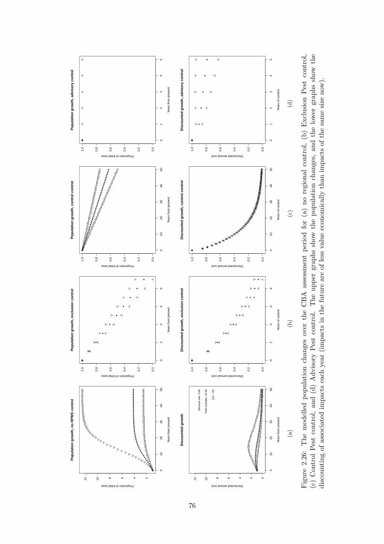
●●
●●
●●
●●
●●
●●
●●
●●
●●
●●
●●
●●
●●
●●
●●
●●
●●
●●
●●
●●
●●
●●
●●
●●
●●
●
010
2030
4050
24681012
Popu
latio
n gr
owth
, no
RPM
S co
ntro
l
Year
s fro
m p
rese
nt
Proportion of initial area
●●
●●
●●
●●
●●
●●
●●
●●
●●
●●
●●
●●
●●
●●
●●
●●
●●
●●
●●
●●
●●
●●
●●
●●
●●
●
010
2030
4050
024681012
Dis
coun
ted
grow
th
Year
s fro
m p
rese
nt
Discounted annual cost
Dis
coun
t rat
e: 0
.08
Tota
l mul
tiplie
r: 32
.99
(23−−7
0)
(a)
●
●
●
●
●
●
●
●
●
●
02
46
8
0.0
0.2
0.4
0.6
0.8
1.0
Popu
latio
n gr
owth
, exc
lusi
on c
ontro
l
Year
s fro
m p
rese
ntProportion of initial area
●
●
●
●
●
●
●
●
●
●
02
46
8
0.0
0.2
0.4
0.6
0.8
1.0
Dis
coun
ted
grow
th, e
xclu
sion
con
trol
Year
s of
con
trol
Discounted annual cost
(b)
●●
●●
●●
●●
●●
●●
●●
●●
●●
●●
●●
●●
●●
●●
●●
●●
●●
●●
●●
●●
●●
●●
●●
●●
●●
●
010
2030
4050
0.0
0.2
0.4
0.6
0.8
1.0
Popu
latio
n gr
owth
, con
trol c
ontro
l
Year
s fro
m p
rese
nt
Proportion of initial area
●
●
●
●
●
●
●
●
●
●
●
●
●
●
●
●●
●●
●●
●●
●●
●●
●●
●●
●●
●●
●●
●●
●●
●●
●●
●●
●●
●●
010
2030
4050
0.0
0.2
0.4
0.6
0.8
1.0
Dis
coun
ted
grow
th, c
ontro
l con
trol
Year
s of
con
trol
Discounted annual cost
(c)
●
●
●
●
●
●
01
23
45
0.0
0.2
0.4
0.6
0.8
1.0
Popu
latio
n gr
owth
, adv
isor
y co
ntro
l
Year
s fro
m p
rese
nt
Proportion of initial area
●
●
●
●
●
●
01
23
45
0.0
0.2
0.4
0.6
0.8
1.0
Dis
coun
ted
grow
th, a
dvis
ory
cont
rol
Year
s of
con
trol
Discounted annual cost
(d)
Fig
ure
2.26
:T
hem
odel
led
popu
lati
onch
ange
sov
erth
eC
BA
asse
ssm
ent
peri
odfo
r(a
)no
regi
onal
cont
rol,
(b)
Exc
lusi
onPes
tco
ntro
l,(c
)C
ontr
olPes
tco
ntro
l,an
d(d
)A
dvis
ory
Pes
tco
ntro
l.T
heup
per
grap
hssh
owth
epo
pula
tion
chan
ges,
and
the
low
ergr
aphs
show
the
disc
ount
ing
ofas
soci
ated
impa
cts
each
year
(im
pact
sin
the
futu
rear
eof
less
valu
eec
onom
ical
lyth
anim
pact
sof
the
sam
esi
zeno
w).
76

2.1.15 Gorse (Ulex europaeus)
Proposed RPMS Category: Advisory
Overall impact: Moderate
Table 2.110: Relevant biology
Attribute DescriptionForm Sharply spiny perennial shrub up to 4 m tall, leaves reduced to a spine-
like tip with a very deep tap root and extensive lateral roots.Habitat Grasslands, shrubland, forest margins, hill country, coastal habitats,
wastelands, optimum growth on low fertility soils.Regional distribution Widespread throughout region.Competitive ability Fast growth and being a nitrogen fixer means it can compete e↵ectively
with tree seedlings.Reproductive ability Seeds have hard coat, can be dormant for up to 30 years. Huge seed
bank in soil (estimated 20,000 seeds/m2).Dispersal methods Most seeds fall close to parent plant but may be ejected up to 6 m. Also
spread by water, birds, road making gravel and machinery.Resistance to control Di�cult to control on infertile and steep land, best controlled by com-
bination of methods.Benefits Can increase soil nitrogen and act as a nursery crop to facilitate regen-
eration of native forest on cleared land.
Table 2.111: Impact evaluation
Category Currentimpact
Potentialimpact
Comment Source
Species diversity L M Forms dense stands, out-competes low-growing species. Increases soil nitrogen,may induce succession to forest, to thedetriment of specialised plants (e.g. herbs,orchids, low ferns). Native forest succes-sion through gorse is vegetatively di↵er-ent and of lower diversity than successionthrough kanuka.
1, 2, 3,4, 5, 6
Threatened species - M 4Soil resources - - 7Water quality L L Increases nitrogen leaching into water-
ways.4
Production M H Spines pull fleece and lower value of wool. 3, 4, 5,8
International trade - - 7Human health - - 7Recreation M M Prickly spines restrict access. 7Maori culture - L Restricts access to cultural sites (e.g.
waahi tapu, urupa).4
Source: 1: Lee et al. (1986), 2: Hill et al. (2001), 3: Williams & Timmins (2002), 4: Craw (2000), 5:Environment Bay of Plenty (2005d), 6: Sullivan et al. (2007), 7: Severinsen (2003), 8: Roy et al. (2004)
77

Gorse CBA results
The following are results for cost-benefit analyses for four scenarios, no regional RPMS control,RPMS control as an Exclusion Pest, RPMS control as a Control Pest, and RPMS control as anAdvisory Pest. For the purposes of the CBA calculations, the pest is assumed to continue expandingwith no regional RPMS control, its spread is assumed to be near-arrested under Advisory Controlbut not reduced, and it is assumed to be successfully reduced to the expected smaller extent whenlisted as a Control Pest, more so as an Exclusion pest.
Table 2.112: Gorse CBA results for four RPMS scenarios, presented as net present value(NPV, $) over 50 years. The expenditure refers to regional expenditure under the RPMS.Minimum and maximum values are in brackets beneath average values.
Scenario Pest impacts Control benefit Expenditure Net benefitNo RPMS 229,103,366 0 0 -229,103,366
(57,016,320–934,996,589) (-57,016,320 – -934,996,589)
Exclusion Pest 51,088,840 178,014,526 20,644,715 157,369,811(17,335,202–84,842,477) (39,681,118–850,154,112) (19,036,403 – 829,509,397)
Control Pest 98,094,788 131,008,578 808,584 130,199,994(32,550,971–166,497,158) (24,465,349–768,499,431) (23,656,765 – 767,690,847)
Advisory Pest 40,593,016 188,510,350 26,424 188,483,926(12,537,482–73,463,106) (44,478,838–861,533,483) (44,452,414 – 861,507,059)
Table 2.113: Gorse CBA base assumptions.
Base assumptions ValuesCurrent area infested (ha) 55,770
Total area potentially infested (ha) 173,453 (57,885–289,022)
Years from naturalisation to total area 25Assessment duration (yr) 50
Weighted average impact per hectare of infested land ($/ha) 137.96 (46.81–229.12)
Any benefits provided by the weed 1Discount rate 0.08
Table 2.114: Gorse RPMS Exclusion Pest assumptions.
Exclusion Pest assumptions ValuesYears to achieve objectives 9
Final area infested (ha) 52,981.5 (52,981.5–52,981.5)
Table 2.115: Gorse RPMS Control Pest assumptions.
Control Pest assumptions ValuesYears to achieve objectives 50
Final area infested (ha) 64,136 (69,712–58,558)
Table 2.116: Gorse RPMS Advisory Pest assumptions.
Advisory Pest assumptions ValuesYears to achieve objectives 5
Final area infested (ha) 71,107 (83,655–58,558)
78

Table 2.117: Gorse estimated total annual cost of di↵erent RPMS scenarios (includesinspection, control, monitoring, enforcement, administration etc.). Subsequent years areassumed to have the same value as the last year listed.
Exclusion Pest Control Pest Advisory PestYear Total Costs Total Costs Total Costs1.00 3,060,000 61,200 2,000
Gorse conclusions
In the absence of regional control, the projected total regional damage in net present value is-$229,103,366 over the next 50 years (the minimum projected impact is -$57,016,320).
Managing Gorse as an Exclusion pest has a projected net benefit to the region of $157,369,811.Since this is positive, this means that this management scenario meets the requirements of Section72(1a) of the Act.
Managing Gorse as a Control pest has a projected net benefit to the region of $130,199,994. Sincethis is positive, this means that this management scenario meets the requirements of Section 72(1a)of the Act.
Managing Gorse as an Advisory pest has a projected net benefit to the region of $188,483,926.Since this is positive, this means that this management scenario meets the requirements of Section72(1a) of the Act.
The proposed management scenario for Gorse, Advisory, therefore meets the requirements of Sec-tion 72(1a) of the Act.
79

−20 −10 0 10 20
0.0
0.2
0.4
0.6
0.8
1.0
Calibrated logistic growth curve, no RPMS control
Years from present
Prop
ortio
n of
max
imum
ext
ent
Current extent (ha): 55,770
Potential extent (ha): 173,453
(57,885−−289,022)
Time to potential (yr): 25
Current prop. of potential: 0.578
Figure 2.27: The modelled pest spread until it reaches its anticipated maximum extent.Shown are the results of the average (solid line), minimum (dotted line), and maximum(dashed line) scenarios. (A horizontal line means that the pest has already reached itsmaximum extent.) The vertical dotted-dashed lines indicate the CBA assessment periodused in this report.
80

●
●
●
●●
●●
●●
●●
●●
●●
●●
●●
●●
●●
●●
●●
●●
●●
●●
●●
●●
●●
●●
●●
●●
●●
●●
●●
010
2030
4050
12345
Popu
latio
n gr
owth
, no
RPM
S co
ntro
l
Year
s fro
m p
rese
nt
Proportion of initial area
●●
●●
●●
●●
●●
●●
●●
●●
●●
●●
●●
●●
●●
●●
●●
●●
●●
●●
●●
●●
●●
●●
●●
●●
●●
●
010
2030
4050
012345
Dis
coun
ted
grow
th
Year
s fro
m p
rese
nt
Discounted annual cost
Dis
coun
t rat
e: 0
.08
Tota
l mul
tiplie
r: 19
.99
(14−−4
9)
(a)
●●
●●
●●
●●
●●
02
46
8
0.0
0.2
0.4
0.6
0.8
1.0
Popu
latio
n gr
owth
, exc
lusi
on c
ontro
l
Year
s fro
m p
rese
ntProportion of initial area
●
●
●
●
●
●
●
●
●
●
02
46
8
0.0
0.2
0.4
0.6
0.8
1.0
Dis
coun
ted
grow
th, e
xclu
sion
con
trol
Year
s of
con
trol
Discounted annual cost
(b)
●●
●●
●●
●●
●●
●●
●●
●●
●●
●●
●●
●●
●●
●●
●●
●●
●●
●●
●●
●●
●●
●●
●●
●●
●●
●
010
2030
4050
0.0
0.2
0.4
0.6
0.8
1.0
1.2
Popu
latio
n gr
owth
, con
trol c
ontro
l
Year
s fro
m p
rese
nt
Proportion of initial area
●
●
●
●
●
●
●
●
●
●
●
●
●
●
●
●
●●
●●
●●
●●
●●
●●
●●
●●
●●
●●
●●
●●
●●
●●
●●
●●
●●
●
010
2030
4050
0.0
0.2
0.4
0.6
0.8
1.0
Dis
coun
ted
grow
th, c
ontro
l con
trol
Year
s of
con
trol
Discounted annual cost
(c)
●
●
●
●
●
●
01
23
45
0.0
0.5
1.0
1.5
Popu
latio
n gr
owth
, adv
isor
y co
ntro
l
Year
s fro
m p
rese
nt
Proportion of initial area
●
●
●
●
●
●
01
23
45
0.0
0.2
0.4
0.6
0.8
1.0
Dis
coun
ted
grow
th, a
dvis
ory
cont
rol
Year
s of
con
trol
Discounted annual cost
(d)
Fig
ure
2.28
:T
hem
odel
led
popu
lati
onch
ange
sov
erth
eC
BA
asse
ssm
ent
peri
odfo
r(a
)no
regi
onal
cont
rol,
(b)
Exc
lusi
onPes
tco
ntro
l,(c
)C
ontr
olPes
tco
ntro
l,an
d(d
)A
dvis
ory
Pes
tco
ntro
l.T
heup
per
grap
hssh
owth
epo
pula
tion
chan
ges,
and
the
low
ergr
aphs
show
the
disc
ount
ing
ofas
soci
ated
impa
cts
each
year
(im
pact
sin
the
futu
rear
eof
less
valu
eec
onom
ical
lyth
anim
pact
sof
the
sam
esi
zeno
w).
81

2.1.16 Green goddess lily (Zantedeschia aethiopica “Green goddess”)
Proposed RPMS Category: Control
Overall impact: Moderate
Table 2.118: Relevant biology
Attribute DescriptionForm Robust, persistent, evergreen, clump-forming perennial herb ¡1.5m tall.
Large arrow-shaped shiny green leaves. White, erect, funnel-shaped‘flower’ (Aug-Jan, occasionally other times of year) of central yellowspike and white outer modified leaf.
Habitat Heavily disturbed shrubland and forest, damp areas with low cover, re-generating ex-pasture.
Regional distribution Common in Tauranga district.Competitive ability Long-lived, smothers ground in open sites on most soil types. Persists
under regenerating canopy. Drought-resistant once established. Formsdense patches excluding other plants. Poisonous, avoided by livestock,dominates grazed sites.
Reproductive ability Produces viable seed.Dispersal methods Water, also planted by humans.Resistance to control Digging often leaves root fragments and dropped tuber pieces which
resprout. Regrows after mowing.
Table 2.119: Impact evaluation
Category Currentimpact
Potentialimpact
Comment Source
Species diversity M H Forms dense patches in wetlands, smoth-ers ground and excludes other species, pre-venting regeneration.
1
Threatened species L M 1Soil resources - L Potentially will impact on hydrology. 2Water quality - -Production L M Poisonous (foliage avoided by livestock). 1, 3International trade - -Human health M H Highly poisonous, causes shock, convul-
sions, death.3, 4
Recreation - -Maori culture - L Unsightly, poisonous plant near water-
ways and cultural sites.1
Source: 1: Auckland Regional Council (2010a), 2: Stahl (2009), 3: Roy et al. (2004), 4: EnvironmentBay of Plenty (2004b)
82

Green goddess lily CBA results
The following are results for cost-benefit analyses for four scenarios, no regional RPMS control,RPMS control as an Exclusion Pest, RPMS control as a Control Pest, and RPMS control as anAdvisory Pest. For the purposes of the CBA calculations, the pest is assumed to continue expandingwith no regional RPMS control, its spread is assumed to be near-arrested under Advisory Controlbut not reduced, and it is assumed to be successfully reduced to the expected smaller extent whenlisted as a Control Pest, more so as an Exclusion pest.
Table 2.120: Green goddess lily CBA results for four RPMS scenarios, presented as netpresent value (NPV, $) over 50 years. The expenditure refers to regional expenditureunder the RPMS. Minimum and maximum values are in brackets beneath average values.
Scenario Pest impacts Control benefit Expenditure Net benefitNo RPMS 1,258,010 0 0 -1,258,010
(350,146–5,734,094) (-350,146 – -5,734,094)
Exclusion Pest 646 1,257,364 3,373,319 -2,115,955(195–1,018) (349,951–5,733,076) (-3,023,368 – 2,359,757)
Control Pest 1,710 1,256,300 132,122 1,124,178(491–2,853) (349,655–5,731,241) (217,533 – 5,599,119)
Advisory Pest 872 1,257,138 13,212 1,243,926(221–1,639) (349,925–5,732,455) (336,713 – 5,719,243)
Table 2.121: Green goddess lily CBA base assumptions.
Base assumptions ValuesCurrent area infested (ha) 20
Total area potentially infested (ha) 103,837 (35,106–172,567)
Years from naturalisation to total area 75Assessment duration (yr) 50
Weighted average impact per hectare of infested land ($/ha) 7.59 (2.11–13.06)
Any benefits provided by the weed 0Discount rate 0.08
Table 2.122: Green goddess lily RPMS Exclusion Pest assumptions.
Exclusion Pest assumptions ValuesYears to achieve objectives 9
Final area infested (ha) 2.5 (0–5)
Table 2.123: Green goddess lily RPMS Control Pest assumptions.
Control Pest assumptions ValuesYears to achieve objectives 50
Final area infested (ha) 12 (10–15)
Table 2.124: Green goddess lily RPMS Advisory Pest assumptions.
Advisory Pest assumptions ValuesYears to achieve objectives 5
83
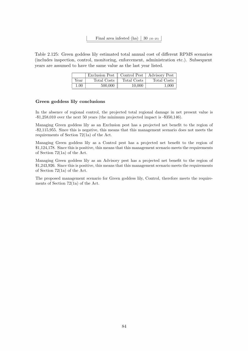
Final area infested (ha) 30 (35–25)
Table 2.125: Green goddess lily estimated total annual cost of di↵erent RPMS scenarios(includes inspection, control, monitoring, enforcement, administration etc.). Subsequentyears are assumed to have the same value as the last year listed.
Exclusion Pest Control Pest Advisory PestYear Total Costs Total Costs Total Costs1.00 500,000 10,000 1,000
Green goddess lily conclusions
In the absence of regional control, the projected total regional damage in net present value is-$1,258,010 over the next 50 years (the minimum projected impact is -$350,146).
Managing Green goddess lily as an Exclusion pest has a projected net benefit to the region of-$2,115,955. Since this is negative, this means that this management scenario does not meets therequirements of Section 72(1a) of the Act.
Managing Green goddess lily as a Control pest has a projected net benefit to the region of$1,124,178. Since this is positive, this means that this management scenario meets the requirementsof Section 72(1a) of the Act.
Managing Green goddess lily as an Advisory pest has a projected net benefit to the region of$1,243,926. Since this is positive, this means that this management scenario meets the requirementsof Section 72(1a) of the Act.
The proposed management scenario for Green goddess lily, Control, therefore meets the require-ments of Section 72(1a) of the Act.
84
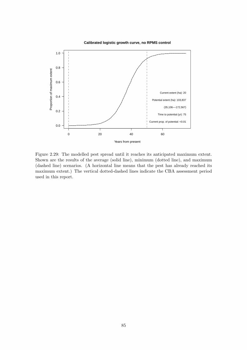
0 20 40 60
0.0
0.2
0.4
0.6
0.8
1.0
Calibrated logistic growth curve, no RPMS control
Years from present
Prop
ortio
n of
max
imum
ext
ent
Current extent (ha): 20
Potential extent (ha): 103,837
(35,106−−172,567)
Time to potential (yr): 75
Current prop. of potential: <0.01
Figure 2.29: The modelled pest spread until it reaches its anticipated maximum extent.Shown are the results of the average (solid line), minimum (dotted line), and maximum(dashed line) scenarios. (A horizontal line means that the pest has already reached itsmaximum extent.) The vertical dotted-dashed lines indicate the CBA assessment periodused in this report.
85

●●
●●
●●
●●
●●
●●
●●
●●
●●
●●
●●
●●
●●
●●
●●
●●
●●
●●
●●
●●
●●
●●
●●
●●
●●
●
010
2030
4050
0
2000
4000
6000
8000
Popu
latio
n gr
owth
, no
RPM
S co
ntro
l
Year
s fro
m p
rese
nt
Proportion of initial area
●●
●●
●●
●●
●●
●●
●●
●●
●●
●●
●●
●●
●●
●●
●●
●●
●●
●●
●●
●●
●●
●●
●●
●●
●●
●
010
2030
4050
0
2000
4000
6000
8000
Dis
coun
ted
grow
th
Year
s fro
m p
rese
nt
Discounted annual cost
Dis
coun
t rat
e: 0
.08
Tota
l mul
tiplie
r: 19
58.7
9
(119
0−−5
792)
(a)
●
●
●
●
●
●
●
●
●
●
02
46
8
0.0
0.2
0.4
0.6
0.8
1.0
Popu
latio
n gr
owth
, exc
lusi
on c
ontro
l
Year
s fro
m p
rese
ntProportion of initial area
●
●
●
●
●
●
●
●
●
●
02
46
8
0.0
0.2
0.4
0.6
0.8
1.0
Dis
coun
ted
grow
th, e
xclu
sion
con
trol
Year
s of
con
trol
Discounted annual cost
(b)
●●
●●
●●
●●
●●
●●
●●
●●
●●
●●
●●
●●
●●
●●
●●
●●
●●
●●
●●
●●
●●
●●
●●
●●
●●
●
010
2030
4050
0.0
0.2
0.4
0.6
0.8
1.0
Popu
latio
n gr
owth
, con
trol c
ontro
l
Year
s fro
m p
rese
nt
Proportion of initial area
●
●
●
●
●
●
●
●
●
●
●
●
●
●
●
●●
●●
●●
●●
●●
●●
●●
●●
●●
●●
●●
●●
●●
●●
●●
●●
●●
●●
010
2030
4050
0.0
0.2
0.4
0.6
0.8
1.0
Dis
coun
ted
grow
th, c
ontro
l con
trol
Year
s of
con
trol
Discounted annual cost
(c)
●
●
●
●
●
●
01
23
45
0.0
0.5
1.0
1.5
Popu
latio
n gr
owth
, adv
isor
y co
ntro
l
Year
s fro
m p
rese
nt
Proportion of initial area
●
●●
●●
●
01
23
45
0.0
0.2
0.4
0.6
0.8
1.0
Dis
coun
ted
grow
th, a
dvis
ory
cont
rol
Year
s of
con
trol
Discounted annual cost
(d)
Fig
ure
2.30
:T
hem
odel
led
popu
lati
onch
ange
sov
erth
eC
BA
asse
ssm
ent
peri
odfo
r(a
)no
regi
onal
cont
rol,
(b)
Exc
lusi
onPes
tco
ntro
l,(c
)C
ontr
olPes
tco
ntro
l,an
d(d
)A
dvis
ory
Pes
tco
ntro
l.T
heup
per
grap
hssh
owth
epo
pula
tion
chan
ges,
and
the
low
ergr
aphs
show
the
disc
ount
ing
ofas
soci
ated
impa
cts
each
year
(im
pact
sin
the
futu
rear
eof
less
valu
eec
onom
ical
lyth
anim
pact
sof
the
sam
esi
zeno
w).
86
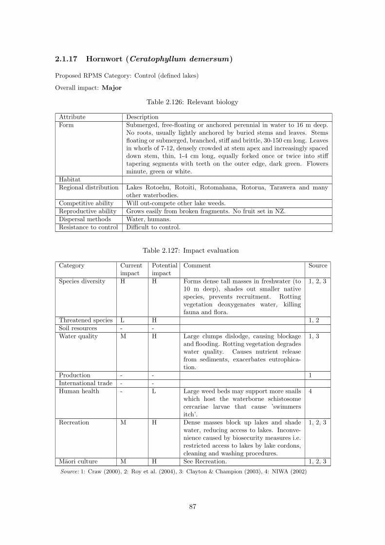
2.1.17 Hornwort (Ceratophyllum demersum)
Proposed RPMS Category: Control (defined lakes)
Overall impact: Major
Table 2.126: Relevant biology
Attribute DescriptionForm Submerged, free-floating or anchored perennial in water to 16 m deep.
No roots, usually lightly anchored by buried stems and leaves. Stemsfloating or submerged, branched, sti↵ and brittle, 30-150 cm long. Leavesin whorls of 7-12, densely crowded at stem apex and increasingly spaceddown stem, thin, 1-4 cm long, equally forked once or twice into sti↵tapering segments with teeth on the outer edge, dark green. Flowersminute, green or white.
HabitatRegional distribution Lakes Rotoehu, Rotoiti, Rotomahana, Rotorua, Tarawera and many
other waterbodies.Competitive ability Will out-compete other lake weeds.Reproductive ability Grows easily from broken fragments. No fruit set in NZ.Dispersal methods Water, humans.Resistance to control Di�cult to control.
Table 2.127: Impact evaluation
Category Currentimpact
Potentialimpact
Comment Source
Species diversity H H Forms dense tall masses in freshwater (to10 m deep), shades out smaller nativespecies, prevents recruitment. Rottingvegetation deoxygenates water, killingfauna and flora.
1, 2, 3
Threatened species L H 1, 2Soil resources - -Water quality M H Large clumps dislodge, causing blockage
and flooding. Rotting vegetation degradeswater quality. Causes nutrient releasefrom sediments, exacerbates eutrophica-tion.
1, 3
Production - - 1International trade - -Human health - L Large weed beds may support more snails
which host the waterborne schistosomecercariae larvae that cause ’swimmersitch’.
4
Recreation M H Dense masses block up lakes and shadewater, reducing access to lakes. Inconve-nience caused by biosecurity measures i.e.restricted access to lakes by lake cordons,cleaning and washing procedures.
1, 2, 3
Maori culture M H See Recreation. 1, 2, 3Source: 1: Craw (2000), 2: Roy et al. (2004), 3: Clayton & Champion (2003), 4: NIWA (2002)
87

Hornwort CBA results
Since Hornwort is currently absent from the defined area, it is di�cult to accurately quantify thecosts and benefits of current and proposed e↵orts to continue to exclude the species. If the specieswere to invade this year and spread in the defined area, without regional control for the next 50years, the total pest impacts over this period in net present value are calculated to be $163,994($109,329–$218,659). This can be compared with the calculated net present value of the proposedannual expenditure on control over this same period of $981,146 (to exclude the Control pest fromthe defined areas). Note that this comparison does not take into account whether or not theproposed level of expenditure is adequate to have a high probability of excluding the species overthis period. Given the broad experience of the biosecurity sta↵ at Environment Bay of Plenty, weassume that it will be.
The following tables provide the parameters used in this cost-benefit analysis.
Table 2.128: Hornwort CBA base assumptions.
Base assumptions ValuesCurrent area infested (ha) 0.25
Total area potentially infested (ha) 1,441 (1,441–1,441)
Years from naturalisation to total area 25Assessment duration (yr) 50
Weighted average impact per hectare of infested land ($/ha) 18.75 (12.5–25)
Any benefits provided by the weed 0Discount rate 0.08
Table 2.129: Hornwort estimated total annual cost of the proposed RPMS scenario (in-cludes inspection, control, monitoring, enforcement, administration etc.). Subsequentyears are assumed to have the same value as the last year listed.
Exclusion PestYear Total Costs1.00 74,261
Hornwort conclusions
Since the calculated average impact should the species invade is lower than the anticipated expendi-ture on regional surveillance and control, this management scenario fails meets the requirements ofSection 72(1a) of the Act. The assessment of impacts in cost-benefit analyses for non-productionpests is inherently di�cult and if the Council decides that the value of keeping Hornwort fromthe defined area is worth more than $163,994 over the next 50 years, then this would satisfy therequirements of Section 72(1a) the Act.
While the projected impacts are worth less than the proposed control for hornwort in ourCBAresult, hornwort is a well recognised and clearly damaging lake weed and we are skeptical thatthe proposed costs would not be justified if the economic values of hornwort impacts on tourism,recreation, and biodiversity were more carefully quantified. If the Council concludes that it isworth more than $74,261 to the region to keep hornwort out of lakes Okareka, Okaro, Okataina,Rerewhakaaitu, Rotokakahi, Rotoma, and Tikitapu, then this satisfied section 72(1a) of the Act.As with all of the lake weeds that are in some region’s lakes and not others, if money is going tobe spent trying to prevent hornwort’s movement into more lakes, a su�cient amount needs to bespent to have a good chance of success. Otherwise, all the will be achieved is delaying the arrivalof the weed into a lake by perhaps a few years.
88

0 5 10 15 20 25
0.0
0.2
0.4
0.6
0.8
1.0
Calibrated logistic growth curve, no RPMS control
Years from present
Prop
ortio
n of
max
imum
ext
ent
Current extent (ha): 0.25
Potential extent (ha): 1,441
Time to potential (yr): 25
Current prop. of potential: <0.01
Figure 2.31: The modelled pest spread until it reaches its anticipated maximum extent.Shown are the results of the average (solid line), minimum (dotted line), and maximum(dashed line) scenarios. (A horizontal line means that the pest has already reached itsmaximum extent.) The vertical dotted-dashed lines indicate the CBA assessment periodused in this report.
89

●●
●●
●●
●●
●
●
●
●
●
●
●
●
●
●
●●
●●
●●
●●
●●
●●
●●
●●
●●
●●
●●
●●
●●
●●
●●
●●
●
010
2030
4050
0
500
1000
1500
Popu
latio
n gr
owth
, no
RPM
S co
ntro
l
Year
s fro
m p
rese
nt
Proportion of initial area
●●
●●
●●
●●
●●
●
●
●
●
●●
●●
●●
●●
●●
●●
●●
●●
●●
●●
●●
●●
●●
●●
●●
●●
●●
●●
●
010
2030
4050
0
500
1000
1500
Dis
coun
ted
grow
th
Year
s fro
m p
rese
nt
Discounted annual cost
Dis
coun
t rat
e: 0
.08
Tota
l mul
tiplie
r: 87
46.3
4
(874
6−−8
746)
(a)
●
●
●
●
●
●
●
●
●
●
02
46
8
0.0
0.2
0.4
0.6
0.8
1.0
Popu
latio
n gr
owth
, exc
lusi
on c
ontro
l
Year
s fro
m p
rese
ntProportion of initial area
●
●
●
●
●
●
●
●
●
●
02
46
8
0.0
0.2
0.4
0.6
0.8
1.0
Dis
coun
ted
grow
th, e
xclu
sion
con
trol
Year
s of
con
trol
Discounted annual cost
(b)
●●
●●
●●
●●
●●
●●
●●
●●
●●
●●
●●
●●
●●
●●
●●
●●
●●
●●
●●
●●
●●
●●
●●
●●
●●
●
010
2030
4050
0.0
0.2
0.4
0.6
0.8
1.0
Popu
latio
n gr
owth
, con
trol c
ontro
l
Year
s fro
m p
rese
nt
Proportion of initial area
●
●
●
●
●
●
●
●
●
●
●
●
●
●
●
●●
●●
●●
●●
●●
●●
●●
●●
●●
●●
●●
●●
●●
●●
●●
●●
●●
●●
010
2030
4050
0.0
0.2
0.4
0.6
0.8
1.0
Dis
coun
ted
grow
th, c
ontro
l con
trol
Year
s of
con
trol
Discounted annual cost
(c)
●
●
●
●
●
●
01
23
45
0.0
0.2
0.4
0.6
0.8
1.0
Popu
latio
n gr
owth
, adv
isor
y co
ntro
l
Year
s fro
m p
rese
nt
Proportion of initial area
●
●
●
●
●
●
01
23
45
0.0
0.2
0.4
0.6
0.8
1.0
Dis
coun
ted
grow
th, a
dvis
ory
cont
rol
Year
s of
con
trol
Discounted annual cost
(d)
Fig
ure
2.32
:T
hem
odel
led
popu
lati
onch
ange
sov
erth
eC
BA
asse
ssm
ent
peri
odfo
r(a
)no
regi
onal
cont
rol,
(b)
Exc
lusi
onPes
tco
ntro
l,(c
)C
ontr
olPes
tco
ntro
l,an
d(d
)A
dvis
ory
Pes
tco
ntro
l.T
heup
per
grap
hssh
owth
epo
pula
tion
chan
ges,
and
the
low
ergr
aphs
show
the
disc
ount
ing
ofas
soci
ated
impa
cts
each
year
(im
pact
sin
the
futu
rear
eof
less
valu
eec
onom
ical
lyth
anim
pact
sof
the
sam
esi
zeno
w).
90

2.1.18 Horse nettle (Solanum carolinense)
Proposed RPMS Category: Exclusion
Overall impact: Moderate
Table 2.130: Relevant biology
Attribute DescriptionForm Small shrub, grows to 1m. Leaves are alternate, elliptic-oblong to oval,
irregularly lobed or coarsely toothed. Both surfaces are covered withfine hairs. Flowers have five petals and are usually white or purple withyellow centers. Fruits resemble tomatoes, immature fruit is dark greenwith light green stripes, turning yellow and wrinkled as it matures.
Habitat Pastures, roadsides, railroad margins, and in disturbed areas and wasteground. Prefers sandy or loamy soils.
Regional distribution Te Puna and Cape Runaway.Competitive abilityReproductive ability Produces viable seed. Each fruit contains around 60 seeds.Dispersal methods Birds disperse seeds.Resistance to control Resistant to many herbicides, in fact herbicide use often selects for hors-
enettle by removing competing weeds. The deep root makes it di�cultto remove.
Table 2.131: Impact evaluation
Category Currentimpact
Potentialimpact
Comment Source
Species diversity - - 1, 2, 3Threatened species - - 1, 2, 3Soil resources - - 1, 2, 3Water quality - - 1, 2, 3Production M H Highly toxic to stock. 1, 2, 3International trade L L Crop contaminant, prohibited seed (nil
tolerance) in imports into Australia.4, 5, 6
Human health L-M M Very dense and di�cult to walk through.Spines penetrate the skin and break o↵when the plant is grasped. All parts of theplant are poisonous, and contain the toxicagent glycoalkaloid which causes depres-sion, excess salivation, diarrhoea, trem-bling, weakness and colic.
1, 2, 3
Recreation L M See Human Health. 1, 2, 3Maori culture - M Obstructs access to cultural sites (e.g.
waahi tapu, urupa).1, 2
Source: 1: Anon. (2009e), 2: Anon. (2009a), 3: Anon. (2009d), 4: Senior (2009), 5: Stahl (2009), 6:Anon. (2009k)
91
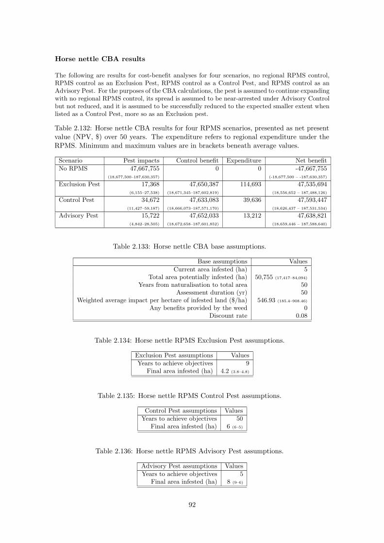
Horse nettle CBA results
The following are results for cost-benefit analyses for four scenarios, no regional RPMS control,RPMS control as an Exclusion Pest, RPMS control as a Control Pest, and RPMS control as anAdvisory Pest. For the purposes of the CBA calculations, the pest is assumed to continue expandingwith no regional RPMS control, its spread is assumed to be near-arrested under Advisory Controlbut not reduced, and it is assumed to be successfully reduced to the expected smaller extent whenlisted as a Control Pest, more so as an Exclusion pest.
Table 2.132: Horse nettle CBA results for four RPMS scenarios, presented as net presentvalue (NPV, $) over 50 years. The expenditure refers to regional expenditure under theRPMS. Minimum and maximum values are in brackets beneath average values.
Scenario Pest impacts Control benefit Expenditure Net benefitNo RPMS 47,667,755 0 0 -47,667,755
(18,677,500–187,630,357) (-18,677,500 – -187,630,357)
Exclusion Pest 17,368 47,650,387 114,693 47,535,694(6,155–27,538) (18,671,345–187,602,819) (18,556,652 – 187,488,126)
Control Pest 34,672 47,633,083 39,636 47,593,447(11,427–59,187) (18,666,073–187,571,170) (18,626,437 – 187,531,534)
Advisory Pest 15,722 47,652,033 13,212 47,638,821(4,842–28,505) (18,672,658–187,601,852) (18,659,446 – 187,588,640)
Table 2.133: Horse nettle CBA base assumptions.
Base assumptions ValuesCurrent area infested (ha) 5
Total area potentially infested (ha) 50,755 (17,417–84,094)
Years from naturalisation to total area 50Assessment duration (yr) 50
Weighted average impact per hectare of infested land ($/ha) 546.93 (185.4–908.46)
Any benefits provided by the weed 0Discount rate 0.08
Table 2.134: Horse nettle RPMS Exclusion Pest assumptions.
Exclusion Pest assumptions ValuesYears to achieve objectives 9
Final area infested (ha) 4.2 (3.8–4.8)
Table 2.135: Horse nettle RPMS Control Pest assumptions.
Control Pest assumptions ValuesYears to achieve objectives 50
Final area infested (ha) 6 (6–5)
Table 2.136: Horse nettle RPMS Advisory Pest assumptions.
Advisory Pest assumptions ValuesYears to achieve objectives 5
Final area infested (ha) 8 (9–6)
92

Table 2.137: Horse nettle estimated total annual cost of di↵erent RPMS scenarios (includesinspection, control, monitoring, enforcement, administration etc.). Subsequent years areassumed to have the same value as the last year listed.
Exclusion Pest Control Pest Advisory PestYear Total Costs Total Costs Total Costs1.00 17,000 3,000 1,000
Horse nettle conclusions
In the absence of regional control, the projected total regional damage in net present value is-$47,667,755 over the next 50 years (the minimum projected impact is -$18,677,500).
Managing Horse nettle as an Exclusion pest has a projected net benefit to the region of $47,535,694.Since this is positive, this means that this management scenario meets the requirements of Section72(1a) of the Act.
Managing Horse nettle as a Control pest has a projected net benefit to the region of $47,593,447.Since this is positive, this means that this management scenario meets the requirements of Section72(1a) of the Act.
Managing Horse nettle as an Advisory pest has a projected net benefit to the region of $47,638,821.Since this is positive, this means that this management scenario meets the requirements of Section72(1a) of the Act.
The proposed management scenario for Horse nettle, Exclusion, therefore meets the requirementsof Section 72(1a) of the Act.
93
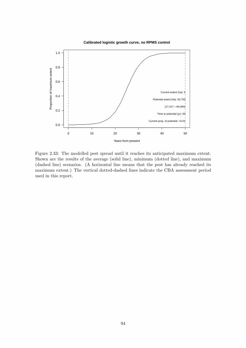
0 10 20 30 40 50
0.0
0.2
0.4
0.6
0.8
1.0
Calibrated logistic growth curve, no RPMS control
Years from present
Prop
ortio
n of
max
imum
ext
ent
Current extent (ha): 5
Potential extent (ha): 50,755
(17,417−−84,094)
Time to potential (yr): 50
Current prop. of potential: <0.01
Figure 2.33: The modelled pest spread until it reaches its anticipated maximum extent.Shown are the results of the average (solid line), minimum (dotted line), and maximum(dashed line) scenarios. (A horizontal line means that the pest has already reached itsmaximum extent.) The vertical dotted-dashed lines indicate the CBA assessment periodused in this report.
94

●●
●●
●●
●●
●●
●●
●●
●●
●●
●●
●●
●
●
●
●
●
●
●●
●●
●●
●●
●●
●●
●●
●●
●●
●●
●●
●
010
2030
4050
0
5000
1000
0
1500
0
Popu
latio
n gr
owth
, no
RPM
S co
ntro
l
Year
s fro
m p
rese
nt
Proportion of initial area
●●
●●
●●
●●
●●
●●
●●
●●
●●
●●
●●
●●
●●
●●
●●
●●
●●
●●
●●
●●
●●
●●
●●
●●
●●
●
010
2030
4050
0
5000
1000
0
1500
0
Dis
coun
ted
grow
th
Year
s fro
m p
rese
nt
Discounted annual cost
Dis
coun
t rat
e: 0
.08
Tota
l mul
tiplie
r: 10
679.
15
(644
6−−3
1118
)
(a)
●●
●●
●●
●●
●●
02
46
8
0.0
0.2
0.4
0.6
0.8
1.0
Popu
latio
n gr
owth
, exc
lusi
on c
ontro
l
Year
s fro
m p
rese
ntProportion of initial area
●
●
●
●
●
●
●
●
●
●
02
46
8
0.0
0.2
0.4
0.6
0.8
1.0
Dis
coun
ted
grow
th, e
xclu
sion
con
trol
Year
s of
con
trol
Discounted annual cost
(b)
●●
●●
●●
●●
●●
●●
●●
●●
●●
●●
●●
●●
●●
●●
●●
●●
●●
●●
●●
●●
●●
●●
●●
●●
●●
●
010
2030
4050
0.0
0.2
0.4
0.6
0.8
1.0
1.2
Popu
latio
n gr
owth
, con
trol c
ontro
l
Year
s fro
m p
rese
nt
Proportion of initial area
●
●
●
●
●
●
●
●
●
●
●
●
●
●
●
●
●●
●●
●●
●●
●●
●●
●●
●●
●●
●●
●●
●●
●●
●●
●●
●●
●●
●
010
2030
4050
0.0
0.2
0.4
0.6
0.8
1.0
Dis
coun
ted
grow
th, c
ontro
l con
trol
Year
s of
con
trol
Discounted annual cost
(c)
●
●
●
●
●
●
01
23
45
0.0
0.5
1.0
1.5
Popu
latio
n gr
owth
, adv
isor
y co
ntro
l
Year
s fro
m p
rese
nt
Proportion of initial area
●
●●
●●
●
01
23
45
0.0
0.2
0.4
0.6
0.8
1.0
Dis
coun
ted
grow
th, a
dvis
ory
cont
rol
Year
s of
con
trol
Discounted annual cost
(d)
Fig
ure
2.34
:T
hem
odel
led
popu
lati
onch
ange
sov
erth
eC
BA
asse
ssm
ent
peri
odfo
r(a
)no
regi
onal
cont
rol,
(b)
Exc
lusi
onPes
tco
ntro
l,(c
)C
ontr
olPes
tco
ntro
l,an
d(d
)A
dvis
ory
Pes
tco
ntro
l.T
heup
per
grap
hssh
owth
epo
pula
tion
chan
ges,
and
the
low
ergr
aphs
show
the
disc
ount
ing
ofas
soci
ated
impa
cts
each
year
(im
pact
sin
the
futu
rear
eof
less
valu
eec
onom
ical
lyth
anim
pact
sof
the
sam
esi
zeno
w).
95

2.1.19 Italian buckthorn (Rhamnus alaternus)
Proposed RPMS Category: Control
Overall impact: Moderate
Table 2.138: Relevant biology
Attribute DescriptionForm Evergreen shrub growing up to 12 m tall.Habitat Coastal areas and bare rock. Also grows on margins of streams, scrub
and forests.Regional distribution Coastal areas only.Competitive ability Grows equally well in shade or in the open, completely dominating many
vegetation types. Will fruit under a closed canopy.Reproductive ability 90,000 to 180,000 seeds produced per individual. Separate male and
female plants, which may account for its slow spread to date.Dispersal methods Birds, such as wax eyes, readily disperse the small fruit. Seeds have 80%
viability.Resistance to control Can be controlled using herbicides and hand pulling young plants. Con-
trol is di�cult in many of the steep coastal sites.Benefits Erosion control, holding up steep banks.
Table 2.139: Impact evaluation
Category Currentimpact
Potentialimpact
Comment Source
Species diversity M M Forms dense stands, dominates many veg-etation types, prevents recruitment.
1, 2, 3
Threatened species L M 1, 2, 3Soil resources - - 4Water quality - - 4Production - L Excludes pasture species. 3International trade - - 4Human health - - 4Recreation - - 4Maori culture L M Obstructs access to cultural sites (e.g.
waahi tapu, urupa).4
Source: 1: Craw (2000), 2: Ministry of Agriculture and Forestry (2008), 3: Anon. (2005a), 4: Severinsen(2003)
96

Italian buckthorn CBA results
The following are results for cost-benefit analyses for four scenarios, no regional RPMS control,RPMS control as an Exclusion Pest, RPMS control as a Control Pest, and RPMS control as anAdvisory Pest. For the purposes of the CBA calculations, the pest is assumed to continue expandingwith no regional RPMS control, its spread is assumed to be near-arrested under Advisory Controlbut not reduced, and it is assumed to be successfully reduced to the expected smaller extent whenlisted as a Control Pest, more so as an Exclusion pest.
Table 2.140: Italian buckthorn CBA results for four RPMS scenarios, presented as netpresent value (NPV, $) over 50 years. The expenditure refers to regional expenditureunder the RPMS. Minimum and maximum values are in brackets beneath average values.
Scenario Pest impacts Control benefit Expenditure Net benefitNo RPMS 2,218,273 0 0 -2,218,273
(316,160–11,629,410) (-316,160 – -11,629,410)
Exclusion Pest 360 2,217,913 2,023,992 193,921(134–545) (316,026–11,628,865) (-1,707,966 – 9,604,873)
Control Pest 952 2,217,321 79,273 2,138,048(337–1,527) (315,823–11,627,883) (236,550 – 11,548,610)
Advisory Pest 441 2,217,832 13,212 2,204,620(167–657) (315,993–11,628,753) (302,781 – 11,615,541)
Table 2.141: Italian buckthorn CBA base assumptions.
Base assumptions ValuesCurrent area infested (ha) 46
Total area potentially infested (ha) 142,406 (47,950–236,863)
Years from naturalisation to total area 50Assessment duration (yr) 50
Weighted average impact per hectare of infested land ($/ha) 1.84 (0.63–3.04)
Any benefits provided by the weed 1Discount rate 0.08
Table 2.142: Italian buckthorn RPMS Exclusion Pest assumptions.
Exclusion Pest assumptions ValuesYears to achieve objectives 9
Final area infested (ha) 5.7 (0–11.5)
Table 2.143: Italian buckthorn RPMS Control Pest assumptions.
Control Pest assumptions ValuesYears to achieve objectives 50
Final area infested (ha) 29 (23–34)
Table 2.144: Italian buckthorn RPMS Advisory Pest assumptions.
Advisory Pest assumptions ValuesYears to achieve objectives 5
97

Final area infested (ha) 58 (46–69)
Table 2.145: Italian buckthorn estimated total annual cost of di↵erent RPMS scenarios(includes inspection, control, monitoring, enforcement, administration etc.). Subsequentyears are assumed to have the same value as the last year listed.
Exclusion Pest Control Pest Advisory PestYear Total Costs Total Costs Total Costs1.00 300,000 6,000 1,000
Italian buckthorn conclusions
In the absence of regional control, the projected total regional damage in net present value is-$2,218,273 over the next 50 years (the minimum projected impact is -$316,160).
Managing Italian buckthorn as an Exclusion pest has a projected net benefit to the region of$193,921. Since this is positive, this means that this management scenario meets the requirementsof Section 72(1a) of the Act.
Managing Italian buckthorn as a Control pest has a projected net benefit to the region of $2,138,048.Since this is positive, this means that this management scenario meets the requirements of Section72(1a) of the Act.
Managing Italian buckthorn as an Advisory pest has a projected net benefit to the region of$2,204,620. Since this is positive, this means that this management scenario meets the requirementsof Section 72(1a) of the Act.
The proposed management scenario for Italian buckthorn, Control, therefore meets the require-ments of Section 72(1a) of the Act.
98

0 10 20 30 40 50
0.0
0.2
0.4
0.6
0.8
1.0
Calibrated logistic growth curve, no RPMS control
Years from present
Prop
ortio
n of
max
imum
ext
ent
Current extent (ha): 46
Potential extent (ha): 142,406
(47,950−−236,863)
Time to potential (yr): 50
Current prop. of potential: 0.001
Figure 2.35: The modelled pest spread until it reaches its anticipated maximum extent.Shown are the results of the average (solid line), minimum (dotted line), and maximum(dashed line) scenarios. (A horizontal line means that the pest has already reached itsmaximum extent.) The vertical dotted-dashed lines indicate the CBA assessment periodused in this report.
99
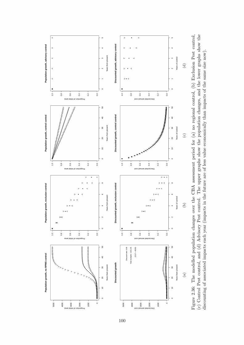
●●
●●
●●
●●
●●
●●
●●
●●
●●
●●
●●
●
●
●
●
●
●
●●
●●
●●
●●
●●
●●
●●
●●
●●
●●
●●
●
010
2030
4050
0
1000
2000
3000
4000
5000
Popu
latio
n gr
owth
, no
RPM
S co
ntro
l
Year
s fro
m p
rese
nt
Proportion of initial area
●●
●●
●●
●●
●●
●●
●●
●●
●●
●●
●●
●●
●●
●●
●●
●●
●●
●●
●●
●●
●●
●●
●●
●●
●●
●
010
2030
4050
0
1000
2000
3000
4000
5000
Dis
coun
ted
grow
th
Year
s fro
m p
rese
nt
Discounted annual cost
Dis
coun
t rat
e: 0
.08
Tota
l mul
tiplie
r: 32
31.0
5
(211
7−−9
528)
(a)
●
●
●
●
●
●
●
●
●
●
02
46
8
0.0
0.2
0.4
0.6
0.8
1.0
Popu
latio
n gr
owth
, exc
lusi
on c
ontro
l
Year
s fro
m p
rese
ntProportion of initial area
●
●
●
●
●
●
●
●
●
●
02
46
8
0.0
0.2
0.4
0.6
0.8
1.0
Dis
coun
ted
grow
th, e
xclu
sion
con
trol
Year
s of
con
trol
Discounted annual cost
(b)
●●
●●
●●
●●
●●
●●
●●
●●
●●
●●
●●
●●
●●
●●
●●
●●
●●
●●
●●
●●
●●
●●
●●
●●
●●
●
010
2030
4050
0.0
0.2
0.4
0.6
0.8
1.0
Popu
latio
n gr
owth
, con
trol c
ontro
l
Year
s fro
m p
rese
nt
Proportion of initial area
●
●
●
●
●
●
●
●
●
●
●
●
●
●
●
●●
●●
●●
●●
●●
●●
●●
●●
●●
●●
●●
●●
●●
●●
●●
●●
●●
●●
010
2030
4050
0.0
0.2
0.4
0.6
0.8
1.0
Dis
coun
ted
grow
th, c
ontro
l con
trol
Year
s of
con
trol
Discounted annual cost
(c)
●
●
●
●
●
●
01
23
45
0.0
0.2
0.4
0.6
0.8
1.0
Popu
latio
n gr
owth
, adv
isor
y co
ntro
l
Year
s fro
m p
rese
nt
Proportion of initial area
●
●
●
●
●
●
01
23
45
0.0
0.2
0.4
0.6
0.8
1.0
Dis
coun
ted
grow
th, a
dvis
ory
cont
rol
Year
s of
con
trol
Discounted annual cost
(d)
Fig
ure
2.36
:T
hem
odel
led
popu
lati
onch
ange
sov
erth
eC
BA
asse
ssm
ent
peri
odfo
r(a
)no
regi
onal
cont
rol,
(b)
Exc
lusi
onPes
tco
ntro
l,(c
)C
ontr
olPes
tco
ntro
l,an
d(d
)A
dvis
ory
Pes
tco
ntro
l.T
heup
per
grap
hssh
owth
epo
pula
tion
chan
ges,
and
the
low
ergr
aphs
show
the
disc
ount
ing
ofas
soci
ated
impa
cts
each
year
(im
pact
sin
the
futu
rear
eof
less
valu
eec
onom
ical
lyth
anim
pact
sof
the
sam
esi
zeno
w).
100

2.1.20 Kudzu vine (Pueraria montana var.lobata)
Proposed RPMS Category: Exclusion
Overall impact: Major
Table 2.146: Relevant biology
Attribute DescriptionForm High climbing vine, often completely covering trees. Stems may reach
up to 10 cm in diameter. Leaves alternate, compound 12-20 cm long, 3individual leaflets 7-10 cm long, oval or may be lobed and fuzzy. Flower,large hanging clusters of pea like, purple to red flowers.
Habitat Open distribution areas, roadsides, forest margins.Regional distribution Three known sites are Pahoia, Te Puke, Matata.Competitive ability Rapid growth will out compete all other plants.Reproductive ability No evidence of viable seed being produced.Dispersal methods Spreads by sending down roots from nearly every node along stems that
contact soil and new crowns develop at these nodes.Resistance to control Di�cult to control because of the large tubers.Benefits Used for erosion control, edible tubers, livestock feed, medicinal uses,
making soap, lotions
Table 2.147: Impact evaluation
Category Currentimpact
Potentialimpact
Comment Source
Species diversity L H High climbing vine, forms dense patchesand smothers all other plants.
1, 2, 3
Threatened species - H 1, 2, 3Soil resources - - 1, 2, 3Water quality - - 3Production - M Smothers trees in plantation forests and
orchards. Prevents access and createssafety hazard during harvest of plantationtrees.
2, 3
International trade - - 3, 4Human health - - 4Recreation - M Dense walls of vines obstruct access to for-
est.2, 3
Maori culture - M See Recreation. 2, 3Source: 1: Anon. (2009c), 2: USDA (2005), 3: Anon. (2009i), 4: Severinsen (2003)
101

Kudzu vine CBA results
The following are results for cost-benefit analyses for four scenarios, no regional RPMS control,RPMS control as an Exclusion Pest, RPMS control as a Control Pest, and RPMS control as anAdvisory Pest. For the purposes of the CBA calculations, the pest is assumed to continue expandingwith no regional RPMS control, its spread is assumed to be near-arrested under Advisory Controlbut not reduced, and it is assumed to be successfully reduced to the expected smaller extent whenlisted as a Control Pest, more so as an Exclusion pest.
Table 2.148: Kudzu vine CBA results for four RPMS scenarios, presented as net presentvalue (NPV, $) over 50 years. The expenditure refers to regional expenditure under theRPMS. Minimum and maximum values are in brackets beneath average values.
Scenario Pest impacts Control benefit Expenditure Net benefitNo RPMS 4,042,904 0 0 -4,042,904
(895,728–19,589,206) (-895,728 – -19,589,206)
Exclusion Pest 3 4,042,901 10,120 4,032,781(1–5) (895,727–19,589,201) (885,607 – 19,579,081)
Control Pest 8 4,042,896 13,212 4,029,684(2–14) (895,726–19,589,192) (882,514 – 19,575,980)
Advisory Pest 4 4,042,900 6,606 4,036,294(1–6) (895,727–19,589,200) (889,121 – 19,582,594)
Table 2.149: Kudzu vine CBA base assumptions.
Base assumptions ValuesCurrent area infested (ha) 1.5
Total area potentially infested (ha) 142,235 (47,892–236,577)
Years from naturalisation to total area 75Assessment duration (yr) 50
Weighted average impact per hectare of infested land ($/ha) 0.1 (0.1–0.9)
Any benefits provided by the weed 1Discount rate 0.08
Table 2.150: Kudzu vine RPMS Exclusion Pest assumptions.
Exclusion Pest assumptions ValuesYears to achieve objectives 9
Final area infested (ha) 0 (0–0.1)
Table 2.151: Kudzu vine RPMS Control Pest assumptions.
Control Pest assumptions ValuesYears to achieve objectives 50
Final area infested (ha) 1 (0–1)
Table 2.152: Kudzu vine RPMS Advisory Pest assumptions.
Advisory Pest assumptions ValuesYears to achieve objectives 5
Final area infested (ha) 2 (2–2)
102

Table 2.153: Kudzu vine estimated total annual cost of di↵erent RPMS scenarios (includesinspection, control, monitoring, enforcement, administration etc.). Subsequent years areassumed to have the same value as the last year listed.
Exclusion Pest Control Pest Advisory PestYear Total Costs Total Costs Total Costs1.00 1,500 1,000 500
Kudzu vine conclusions
In the absence of regional control, the projected total regional damage in net present value is-$4,042,904 over the next 50 years (the minimum projected impact is -$895,728).
Managing Kudzu vine as an Exclusion pest has a projected net benefit to the region of $4,032,781.Since this is positive, this means that this management scenario meets the requirements of Section72(1a) of the Act.
Managing Kudzu vine as a Control pest has a projected net benefit to the region of $4,029,684.Since this is positive, this means that this management scenario meets the requirements of Section72(1a) of the Act.
Managing Kudzu vine as an Advisory pest has a projected net benefit to the region of $4,036,294.Since this is positive, this means that this management scenario meets the requirements of Section72(1a) of the Act.
The proposed management scenario for Kudzu vine, Exclusion, therefore meets the requirementsof Section 72(1a) of the Act.
103

0 20 40 60
0.0
0.2
0.4
0.6
0.8
1.0
Calibrated logistic growth curve, no RPMS control
Years from present
Prop
ortio
n of
max
imum
ext
ent
Current extent (ha): 1.5
Potential extent (ha): 142,235
(47,892−−236,577)
Time to potential (yr): 75
Current prop. of potential: <0.01
Figure 2.37: The modelled pest spread until it reaches its anticipated maximum extent.Shown are the results of the average (solid line), minimum (dotted line), and maximum(dashed line) scenarios. (A horizontal line means that the pest has already reached itsmaximum extent.) The vertical dotted-dashed lines indicate the CBA assessment periodused in this report.
104

●●
●●
●●
●●
●●
●●
●●
●●
●●
●●
●●
●●
●●
●●
●●
●●
●●
●●
●●
●●
●●
●●
●●
●●
●●
●
010
2030
4050
0
5000
0
1000
00
1500
00
Popu
latio
n gr
owth
, no
RPM
S co
ntro
l
Year
s fro
m p
rese
nt
Proportion of initial area
●●
●●
●●
●●
●●
●●
●●
●●
●●
●●
●●
●●
●●
●●
●●
●●
●●
●●
●●
●●
●●
●●
●●
●●
●●
●
010
2030
4050
0
5000
0
1000
00
1500
00
Dis
coun
ted
grow
th
Year
s fro
m p
rese
nt
Discounted annual cost
Dis
coun
t rat
e: 0
.08
Tota
l mul
tiplie
r: 35
641.
61
(214
29−−
1058
49)
(a)
●
●
●
●
●
●
●
●
●
●
02
46
8
0.0
0.2
0.4
0.6
0.8
1.0
Popu
latio
n gr
owth
, exc
lusi
on c
ontro
l
Year
s fro
m p
rese
ntProportion of initial area
●
●
●
●
●
●
●
●
●
●
02
46
8
0.0
0.2
0.4
0.6
0.8
1.0
Dis
coun
ted
grow
th, e
xclu
sion
con
trol
Year
s of
con
trol
Discounted annual cost
(b)
●●
●●
●●
●●
●●
●●
●●
●●
●●
●●
●●
●●
●●
●●
●●
●●
●●
●●
●●
●●
●●
●●
●●
●●
●●
●
010
2030
4050
0.0
0.2
0.4
0.6
0.8
1.0
Popu
latio
n gr
owth
, con
trol c
ontro
l
Year
s fro
m p
rese
nt
Proportion of initial area
●
●
●
●
●
●
●
●
●
●
●
●
●
●
●
●●
●●
●●
●●
●●
●●
●●
●●
●●
●●
●●
●●
●●
●●
●●
●●
●●
●●
010
2030
4050
0.0
0.2
0.4
0.6
0.8
1.0
Dis
coun
ted
grow
th, c
ontro
l con
trol
Year
s of
con
trol
Discounted annual cost
(c)
●
●
●
●
●
●
01
23
45
0.0
0.2
0.4
0.6
0.8
1.0
Popu
latio
n gr
owth
, adv
isor
y co
ntro
l
Year
s fro
m p
rese
nt
Proportion of initial area
●
●
●
●
●
●
01
23
45
0.0
0.2
0.4
0.6
0.8
1.0
Dis
coun
ted
grow
th, a
dvis
ory
cont
rol
Year
s of
con
trol
Discounted annual cost
(d)
Fig
ure
2.38
:T
hem
odel
led
popu
lati
onch
ange
sov
erth
eC
BA
asse
ssm
ent
peri
odfo
r(a
)no
regi
onal
cont
rol,
(b)
Exc
lusi
onPes
tco
ntro
l,(c
)C
ontr
olPes
tco
ntro
l,an
d(d
)A
dvis
ory
Pes
tco
ntro
l.T
heup
per
grap
hssh
owth
epo
pula
tion
chan
ges,
and
the
low
ergr
aphs
show
the
disc
ount
ing
ofas
soci
ated
impa
cts
each
year
(im
pact
sin
the
futu
rear
eof
less
valu
eec
onom
ical
lyth
anim
pact
sof
the
sam
esi
zeno
w).
105

2.1.21 Lagarosiphon (Lagarosiphon major)
Proposed RPMS Category: Control (defined lakes)
Overall impact: Major
Table 2.154: Relevant biology
Attribute DescriptionForm Submerged, bottom-rooting perennial, reaching to 5 m. Leaves recurved
backwards or downwards, arranged spirally around the stem. Leaves 16x 2 mm, with minute marginal serrations. Flowers tiny, pinkish.
Habitat Rivers, lakes, dunelakes and other still or slow-moving waterbodies withmod-high light.
Regional distribution Lakes Okareka, Okataina, Rerewhakaaitu, Rotoehu, Rotoiti, Rotoma,Rotorua, Tarawera, Tikitapu and many other waterbodies.
Competitive abilityReproductive ability Grows easily from broken fragments. Only female plants found in NZ,
no seed set.Dispersal methods Water, humans.Resistance to control Di�cult to control.
Table 2.155: Impact evaluation
Category Currentimpact
Potentialimpact
Comment Source
Species diversity M H Forms vast deep meadows in freshwaterup to 4 m tall (to 6 m deep), shades outsmaller native species. Rotting vegeta-tion deoxygenates water, killing fauna andflora.
1, 2, 3,4
Threatened species L H Serious threat to dune lakes and nativeaquatic species.
1, 2, 3
Soil resources - -Water quality M H Large clumps dislodge, causing blockage
and flooding. Rotting vegetation degradeswater quality. Causes nutrient releasefrom sediments, exacerbates eutrophica-tion.
1, 3, 4
Production - - 1, 3, 5International trade - -Human health - L Large weed beds may support more snails
which host the waterborne schistosomecercariae larvae that cause ’swimmersitch’.
6
Recreation M H Dense masses block up lakes and shadewater, reducing access to lakes. Inconve-nience caused by biosecurity measures i.e.restricted access to lakes by lake cordons,cleaning and washing procedures.
1, 2, 3,4
Maori culture M H See Recreation. 1, 2, 3,4
Source: 1: Craw (2000), 2: Roy et al. (2004), 3: Anon. (2006c), 4: Clayton & Champion (2003), 5:Department of Conservation (2007), 6: NIWA (2002)
106

Lagarosiphon CBA results
Since Lagarosiphon is currently absent from the defined area, it is di�cult to accurately quantifythe costs and benefits of current and proposed e↵orts to continue to exclude the species. If thespecies were to invade this year and spread in the defined area, without regional control for thenext 50 years, the total pest impacts over this period in net present value are calculated to be$412,940 ($539,742–$442,649). This can be compared with the calculated net present value of theproposed annual expenditure on control over this same period of $245,286 (to exclude the Controlpest from the defined areas). Note that this comparison does not take into account whether or notthe proposed level of expenditure is adequate to have a high probability of excluding the speciesover this period. Given the broad experience of the biosecurity sta↵ at Environment Bay of Plenty,we assume that it will be.
The following tables provide the parameters used in this cost-benefit analysis.
Table 2.156: Lagarosiphon CBA base assumptions.
Base assumptions ValuesCurrent area infested (ha) 0
Total area potentially infested (ha) 147 (147–147)
Years from naturalisation to total area 25Assessment duration (yr) 50
Weighted average impact per hectare of infested land ($/ha) 7.38 (2.5–12.25)
Any benefits provided by the weed 0Discount rate 0.08
Table 2.157: Lagarosiphon estimated total annual cost of the proposed RPMS scenario(includes inspection, control, monitoring, enforcement, administration etc.). Subsequentyears are assumed to have the same value as the last year listed.
Exclusion PestYear Total Costs1.00 18,565
Lagarosiphon conclusions
Since the calculated average impact should the species establish in the defined area is greater thanthe anticipated expenditure, and establishment is likely in the absence of regional surveillance andcontrol, this management scenario meets the requirements of Section 72(1a) of the Act.
107

0 5 10 15 20 25
0.0
0.2
0.4
0.6
0.8
1.0
Calibrated logistic growth curve, no RPMS control
Years from present
Prop
ortio
n of
max
imum
ext
ent
Current extent (ha): 0
Potential extent (ha): 147
Time to potential (yr): 25
Current prop. of potential: <0.01
Figure 2.39: The modelled pest spread until it reaches its anticipated maximum extent.Shown are the results of the average (solid line), minimum (dotted line), and maximum(dashed line) scenarios. (A horizontal line means that the pest has already reached itsmaximum extent.) The vertical dotted-dashed lines indicate the CBA assessment periodused in this report.
108
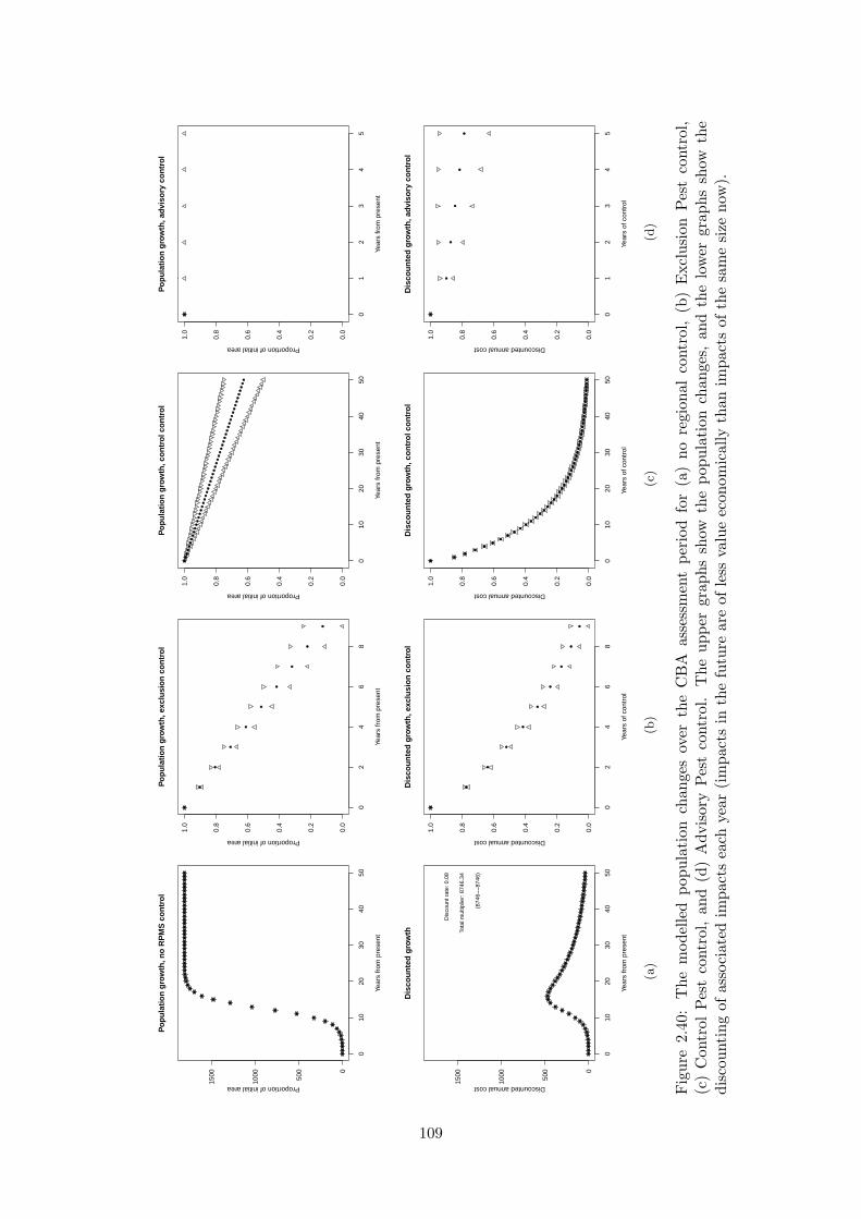
●●
●●
●●
●●
●
●
●
●
●
●
●
●
●
●
●●
●●
●●
●●
●●
●●
●●
●●
●●
●●
●●
●●
●●
●●
●●
●●
●
010
2030
4050
0
500
1000
1500
Popu
latio
n gr
owth
, no
RPM
S co
ntro
l
Year
s fro
m p
rese
nt
Proportion of initial area
●●
●●
●●
●●
●●
●
●
●
●
●●
●●
●●
●●
●●
●●
●●
●●
●●
●●
●●
●●
●●
●●
●●
●●
●●
●●
●
010
2030
4050
0
500
1000
1500
Dis
coun
ted
grow
th
Year
s fro
m p
rese
nt
Discounted annual cost
Dis
coun
t rat
e: 0
.08
Tota
l mul
tiplie
r: 87
46.3
4
(874
6−−8
746)
(a)
●
●
●
●
●
●
●
●
●
●
02
46
8
0.0
0.2
0.4
0.6
0.8
1.0
Popu
latio
n gr
owth
, exc
lusi
on c
ontro
l
Year
s fro
m p
rese
ntProportion of initial area
●
●
●
●
●
●
●
●
●
●
02
46
8
0.0
0.2
0.4
0.6
0.8
1.0
Dis
coun
ted
grow
th, e
xclu
sion
con
trol
Year
s of
con
trol
Discounted annual cost
(b)
●●
●●
●●
●●
●●
●●
●●
●●
●●
●●
●●
●●
●●
●●
●●
●●
●●
●●
●●
●●
●●
●●
●●
●●
●●
●
010
2030
4050
0.0
0.2
0.4
0.6
0.8
1.0
Popu
latio
n gr
owth
, con
trol c
ontro
l
Year
s fro
m p
rese
nt
Proportion of initial area
●
●
●
●
●
●
●
●
●
●
●
●
●
●
●
●●
●●
●●
●●
●●
●●
●●
●●
●●
●●
●●
●●
●●
●●
●●
●●
●●
●●
010
2030
4050
0.0
0.2
0.4
0.6
0.8
1.0
Dis
coun
ted
grow
th, c
ontro
l con
trol
Year
s of
con
trol
Discounted annual cost
(c)
●
●
●
●
●
●
01
23
45
0.0
0.2
0.4
0.6
0.8
1.0
Popu
latio
n gr
owth
, adv
isor
y co
ntro
l
Year
s fro
m p
rese
nt
Proportion of initial area
●
●
●
●
●
●
01
23
45
0.0
0.2
0.4
0.6
0.8
1.0
Dis
coun
ted
grow
th, a
dvis
ory
cont
rol
Year
s of
con
trol
Discounted annual cost
(d)
Fig
ure
2.40
:T
hem
odel
led
popu
lati
onch
ange
sov
erth
eC
BA
asse
ssm
ent
peri
odfo
r(a
)no
regi
onal
cont
rol,
(b)
Exc
lusi
onPes
tco
ntro
l,(c
)C
ontr
olPes
tco
ntro
l,an
d(d
)A
dvis
ory
Pes
tco
ntro
l.T
heup
per
grap
hssh
owth
epo
pula
tion
chan
ges,
and
the
low
ergr
aphs
show
the
disc
ount
ing
ofas
soci
ated
impa
cts
each
year
(im
pact
sin
the
futu
rear
eof
less
valu
eec
onom
ical
lyth
anim
pact
sof
the
sam
esi
zeno
w).
109

2.1.22 Lantana (Lantana camara var.aculeata)
Proposed RPMS Category: Control
Overall impact: Moderate
Table 2.158: Relevant biology
Attribute DescriptionForm Aromatic prickly herbaceous shrub growing to 3 m tall.Habitat Coastal scrubland, islands, cli↵s, foreshores, consolidated dunes, forest
margins, grassland, wasteland, exotic plantations, gardens.Regional distribution Concentrations in urban areas (grown as an ornamental).Competitive ability Very competitive in disturbed, high light conditions, can tolerate wet
and dry.Reproductive ability Prolific seeders.Dispersal methods Spread by birds.Resistance to control Major weed of overseas crops. Can be controlled with herbicide, but
these may a↵ect surrounding vegetation. Biocontrol options have beeninvestigated overseas but to date these are not promising.
Table 2.159: Impact evaluation
Category Currentimpact
Potentialimpact
Comment Source
Species diversity L M Totally smothers and replaces all otherspecies on the ground, causing permanentloss of habitat.
1, 2, 3
Threatened species L M 1Soil resources - - 4Water quality - - 4Production L M Toxic to stock. 1, 2, 3International trade - - 4Human health L-M L Fruit are highly poisonous, causes vomit-
ing, diarrhoea, abdominal pain, sensitivityto light, coma.
3, 5
Recreation - L Dense stands restrict access. 3Maori culture - L Could obstruct access to cultural sites in
coastal areas (e.g. waahi tapu, urupa).3
Source: 1: Craw (2000), 2: Environment Bay of Plenty (2004a), 3: Environment Bay of Plenty (2003),4: Severinsen (2003), 5: Environment Bay of Plenty (2004b)
110
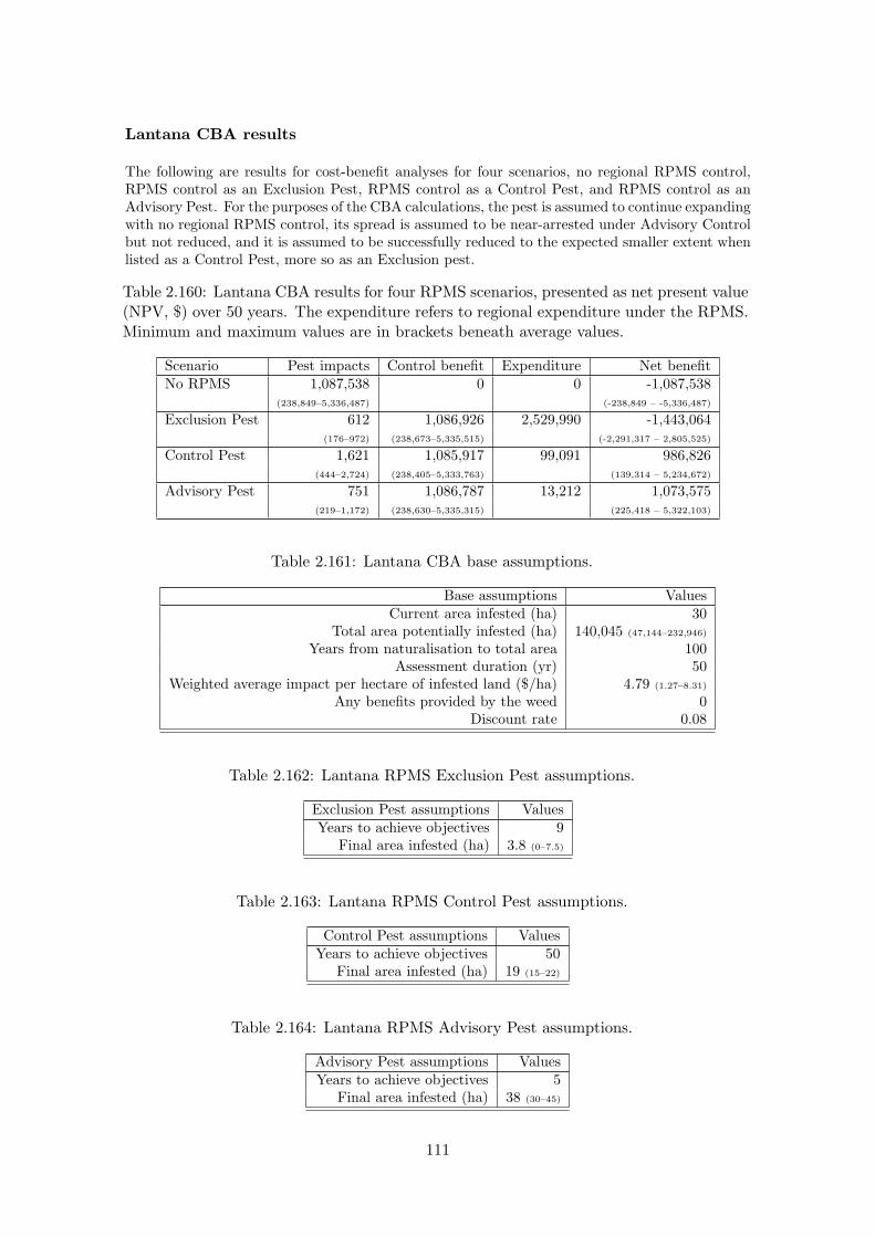
Lantana CBA results
The following are results for cost-benefit analyses for four scenarios, no regional RPMS control,RPMS control as an Exclusion Pest, RPMS control as a Control Pest, and RPMS control as anAdvisory Pest. For the purposes of the CBA calculations, the pest is assumed to continue expandingwith no regional RPMS control, its spread is assumed to be near-arrested under Advisory Controlbut not reduced, and it is assumed to be successfully reduced to the expected smaller extent whenlisted as a Control Pest, more so as an Exclusion pest.
Table 2.160: Lantana CBA results for four RPMS scenarios, presented as net present value(NPV, $) over 50 years. The expenditure refers to regional expenditure under the RPMS.Minimum and maximum values are in brackets beneath average values.
Scenario Pest impacts Control benefit Expenditure Net benefitNo RPMS 1,087,538 0 0 -1,087,538
(238,849–5,336,487) (-238,849 – -5,336,487)
Exclusion Pest 612 1,086,926 2,529,990 -1,443,064(176–972) (238,673–5,335,515) (-2,291,317 – 2,805,525)
Control Pest 1,621 1,085,917 99,091 986,826(444–2,724) (238,405–5,333,763) (139,314 – 5,234,672)
Advisory Pest 751 1,086,787 13,212 1,073,575(219–1,172) (238,630–5,335,315) (225,418 – 5,322,103)
Table 2.161: Lantana CBA base assumptions.
Base assumptions ValuesCurrent area infested (ha) 30
Total area potentially infested (ha) 140,045 (47,144–232,946)
Years from naturalisation to total area 100Assessment duration (yr) 50
Weighted average impact per hectare of infested land ($/ha) 4.79 (1.27–8.31)
Any benefits provided by the weed 0Discount rate 0.08
Table 2.162: Lantana RPMS Exclusion Pest assumptions.
Exclusion Pest assumptions ValuesYears to achieve objectives 9
Final area infested (ha) 3.8 (0–7.5)
Table 2.163: Lantana RPMS Control Pest assumptions.
Control Pest assumptions ValuesYears to achieve objectives 50
Final area infested (ha) 19 (15–22)
Table 2.164: Lantana RPMS Advisory Pest assumptions.
Advisory Pest assumptions ValuesYears to achieve objectives 5
Final area infested (ha) 38 (30–45)
111

Table 2.165: Lantana estimated total annual cost of di↵erent RPMS scenarios (includesinspection, control, monitoring, enforcement, administration etc.). Subsequent years areassumed to have the same value as the last year listed.
Exclusion Pest Control Pest Advisory PestYear Total Costs Total Costs Total Costs1.00 375,000 7,500 1,000
Lantana conclusions
In the absence of regional control, the projected total regional damage in net present value is-$1,087,538 over the next 50 years (the minimum projected impact is -$238,849).
Managing Lantana as an Exclusion pest has a projected net benefit to the region of -$1,443,064.Since this is negative, this means that this management scenario does not meets the requirementsof Section 72(1a) of the Act.
Managing Lantana as a Control pest has a projected net benefit to the region of $986,826. Sincethis is positive, this means that this management scenario meets the requirements of Section 72(1a)of the Act.
Managing Lantana as an Advisory pest has a projected net benefit to the region of $1,073,575.Since this is positive, this means that this management scenario meets the requirements of Section72(1a) of the Act.
The proposed management scenario for Lantana, Control, therefore meets the requirements ofSection 72(1a) of the Act.
112

0 20 40 60 80 100
0.0
0.2
0.4
0.6
0.8
1.0
Calibrated logistic growth curve, no RPMS control
Years from present
Prop
ortio
n of
max
imum
ext
ent
Current extent (ha): 30
Potential extent (ha): 140,045
(47,144−−232,946)
Time to potential (yr): 100
Current prop. of potential: <0.01
Figure 2.41: The modelled pest spread until it reaches its anticipated maximum extent.Shown are the results of the average (solid line), minimum (dotted line), and maximum(dashed line) scenarios. (A horizontal line means that the pest has already reached itsmaximum extent.) The vertical dotted-dashed lines indicate the CBA assessment periodused in this report.
113

●●
●●
●●
●●
●●
●●
●●
●●
●●
●●
●●
●●
●●
●●
●●
●●
●●
●●
●●
●●
●●
●●
●●
●
●
●
●
●
010
2030
4050
0
1000
2000
3000
4000
Popu
latio
n gr
owth
, no
RPM
S co
ntro
l
Year
s fro
m p
rese
nt
Proportion of initial area
●●
●●
●●
●●
●●
●●
●●
●●
●●
●●
●●
●●
●●
●●
●●
●●
●●
●●
●●
●●
●●
●●
●●
●●
●●
●
010
2030
4050
0
1000
2000
3000
4000
Dis
coun
ted
grow
th
Year
s fro
m p
rese
nt
Discounted annual cost
Dis
coun
t rat
e: 0
.08
Tota
l mul
tiplie
r: 59
6.33
(387−−
1769
)
(a)
●
●
●
●
●
●
●
●
●
●
02
46
8
0.0
0.2
0.4
0.6
0.8
1.0
Popu
latio
n gr
owth
, exc
lusi
on c
ontro
l
Year
s fro
m p
rese
ntProportion of initial area
●
●
●
●
●
●
●
●
●
●
02
46
8
0.0
0.2
0.4
0.6
0.8
1.0
Dis
coun
ted
grow
th, e
xclu
sion
con
trol
Year
s of
con
trol
Discounted annual cost
(b)
●●
●●
●●
●●
●●
●●
●●
●●
●●
●●
●●
●●
●●
●●
●●
●●
●●
●●
●●
●●
●●
●●
●●
●●
●●
●
010
2030
4050
0.0
0.2
0.4
0.6
0.8
1.0
Popu
latio
n gr
owth
, con
trol c
ontro
l
Year
s fro
m p
rese
nt
Proportion of initial area
●
●
●
●
●
●
●
●
●
●
●
●
●
●
●
●●
●●
●●
●●
●●
●●
●●
●●
●●
●●
●●
●●
●●
●●
●●
●●
●●
●●
010
2030
4050
0.0
0.2
0.4
0.6
0.8
1.0
Dis
coun
ted
grow
th, c
ontro
l con
trol
Year
s of
con
trol
Discounted annual cost
(c)
●
●
●
●
●
●
01
23
45
0.0
0.2
0.4
0.6
0.8
1.0
Popu
latio
n gr
owth
, adv
isor
y co
ntro
l
Year
s fro
m p
rese
nt
Proportion of initial area
●
●
●
●
●
●
01
23
45
0.0
0.2
0.4
0.6
0.8
1.0
Dis
coun
ted
grow
th, a
dvis
ory
cont
rol
Year
s of
con
trol
Discounted annual cost
(d)
Fig
ure
2.42
:T
hem
odel
led
popu
lati
onch
ange
sov
erth
eC
BA
asse
ssm
ent
peri
odfo
r(a
)no
regi
onal
cont
rol,
(b)
Exc
lusi
onPes
tco
ntro
l,(c
)C
ontr
olPes
tco
ntro
l,an
d(d
)A
dvis
ory
Pes
tco
ntro
l.T
heup
per
grap
hssh
owth
epo
pula
tion
chan
ges,
and
the
low
ergr
aphs
show
the
disc
ount
ing
ofas
soci
ated
impa
cts
each
year
(im
pact
sin
the
futu
rear
eof
less
valu
eec
onom
ical
lyth
anim
pact
sof
the
sam
esi
zeno
w).
114

2.1.23 Marshwort (Nymphoides geminata)
Proposed RPMS Category: Exclusion
Overall impact: Moderate
Table 2.166: Relevant biology
Attribute DescriptionForm Aquatic perennial with branched stolons up to 1 m long usually just
below surface and rounded, floating leaves with V-shaped sinus.Habitat Still water of swamps to fast flowing freshwater streams, lake margins
and small ponds.Regional distribution Eradicated from Lake Okareka, Rotorua.Competitive ability Spreads quickly and out-competes native aquatic plants.Reproductive ability No viable seed produced in New Zealand.Dispersal methods Spreads by branched runners, if a leaf is broken o↵ a new plant will
grow. Spread most commonly through accidental or purposeful humanintervention.
Resistance to control No known suitable herbicide, can be controlled with weed mat for aquaticplants.
Table 2.167: Impact evaluation
Category Currentimpact
Potentialimpact
Comment Source
Species diversity - M Spreads quickly, forms dense mats of float-ing leaves, out-competes native aquaticplants. deoxygenates water killing floraand fauna.
1, 2
Threatened species - L 1, 2, 3Soil resources - - 1Water quality - M Dense mats deoxygenate water. 1, 2Production - - 3International trade - - 3Human health - - 3Recreation - M Dense mats restrict access to waterways
for fishing, swimming, kayaking etc.1, 2
Maori culture - M See Recreation. 1, 2Source: 1: Anon. (2007c), 2: Clayton & Tanner (1985), 3: Severinsen (2003)
115

Marshwort CBA results
Since Marshwort is currently absent from the region, it is di�cult to accurately quantify the costsand benefits of current and proposed e↵orts to continue to exclude the species. If the species wereto invade this year and spread in the region, without regional control for the next 50 years, the totalpest impacts over this period in net present value are calculated to be $17,017 ($2,147–$46,010).This can be compared with the calculated net present value of the proposed annual expenditureon control over this same period of $6,747 (Exclusion pest). Note that this comparison does nottake into account whether or not the proposed level of expenditure is adequate to have a highprobability of excluding the species over this period. Given the broad experience of the biosecuritysta↵ at Environment Bay of Plenty, we assume that it will be.
The following tables provide the parameters used in this cost-benefit analysis.
Table 2.168: Marshwort CBA base assumptions.
Base assumptions ValuesCurrent area infested (ha) 0
Total area potentially infested (ha) 4,216 (1,405–7,027)
Years from naturalisation to total area 100Assessment duration (yr) 50
Weighted average impact per hectare of infested land ($/ha) 1 (1–1)
Any benefits provided by the weed 0Discount rate 0.08
Table 2.169: Marshwort estimated total annual cost of the proposed RPMS scenario (in-cludes inspection, control, monitoring, enforcement, administration etc.). Subsequentyears are assumed to have the same value as the last year listed.
Exclusion PestYear Total Costs1.00 1,000
Marshwort conclusions
Since the calculated average impact should the species invade is greater than the anticipated expen-diture, and regional establishment is likely in the absence of regional surveillance and preparationsfor rapid response, this management scenario meets the requirements of Section 72(1a) of theAct.
116

2.1.24 Nassella tussock (Nassella trichotoma)
Proposed RPMS Category: Exclusion
Overall impact: Major
Table 2.170: Relevant biology
Attribute DescriptionForm Perennial tussock forming grass growing to a height of 50 cm with numer-
ous drooping fine, rough leaves overtopped by slender open seed heads.Habitat Open sites such as sunny dry pasture, stream margins, roadsides and
wasteland. Tolerates a wide range of climates.Regional distribution Confined to one site in Opotiki District.Competitive ability Can form a complete cover in pasture situations.Reproductive ability Can produce up to 100,000 seeds per plant. Seed can remain dormant
in the soil for over 15 years.Dispersal methods Primarily by wind but also stock, machinery, water, hay and as a seed
impurity.Resistance to control Di�cult to control due to large, long-lived seed bank.
Table 2.171: Impact evaluation
Category Currentimpact
Potentialimpact
Comment Source
Species diversity - H Forms pure stands in low-growing plantcommunities, esp. in harsh sites, excludesother species.
1, 2
Threatened species - H 1, 2Soil resources - -Water quality - - 3Production - H Cannot be digested by livestock (forms in-
digestible balls in the stomach). Seedsspoil the fleece.
1, 2
International trade - L Crop contaminant, prohibited seed (niltolerance) in imports into Australia.
4
Human health - - 3Recreation - - 3Maori culture - - 3Source: 1: Craw (2000), 2: Anon. (2004b), 3: Severinsen (2003), 4: Anon. (2009k)
117

Nassella tussock CBA results
The following are results for cost-benefit analyses for four scenarios, no regional RPMS control,RPMS control as an Exclusion Pest, RPMS control as a Control Pest, and RPMS control as anAdvisory Pest. For the purposes of the CBA calculations, the pest is assumed to continue expandingwith no regional RPMS control, its spread is assumed to be near-arrested under Advisory Controlbut not reduced, and it is assumed to be successfully reduced to the expected smaller extent whenlisted as a Control Pest, more so as an Exclusion pest.
Table 2.172: Nassella tussock CBA results for four RPMS scenarios, presented as netpresent value (NPV, $) over 50 years. The expenditure refers to regional expenditureunder the RPMS. Minimum and maximum values are in brackets beneath average values.
Scenario Pest impacts Control benefit Expenditure Net benefitNo RPMS 7,177,008 0 0 -7,177,008
(2,786,207–27,839,851) (-2,786,207 – -27,839,851)
Exclusion Pest 4 7,177,004 6,747 7,170,257(5–4) (2,786,202–27,839,847) (2,779,455 – 27,833,100)
Control Pest 11 7,176,997 6,606 7,170,391(12–11) (2,786,195–27,839,840) (2,779,589 – 27,833,234)
Advisory Pest 5 7,177,003 6,606 7,170,397(6–5) (2,786,201–27,839,846) (2,779,595 – 27,833,240)
Table 2.173: Nassella tussock CBA base assumptions.
Base assumptions ValuesCurrent area infested (ha) 2
Total area potentially infested (ha) 58,294 (20,433–96,155)
Years from naturalisation to total area 75Assessment duration (yr) 50
Weighted average impact per hectare of infested land ($/ha) 1 (1–1)
Any benefits provided by the weed 0Discount rate 0.08
Table 2.174: Nassella tussock RPMS Exclusion Pest assumptions.
Exclusion Pest assumptions ValuesYears to achieve objectives 9
Final area infested (ha) 0.2 (0–0.5)
Table 2.175: Nassella tussock RPMS Control Pest assumptions.
Control Pest assumptions ValuesYears to achieve objectives 50
Final area infested (ha) 1 (1–2)
Table 2.176: Nassella tussock RPMS Advisory Pest assumptions.
Advisory Pest assumptions ValuesYears to achieve objectives 5
118

Final area infested (ha) 2 (2–3)
Table 2.177: Nassella tussock estimated total annual cost of di↵erent RPMS scenarios(includes inspection, control, monitoring, enforcement, administration etc.). Subsequentyears are assumed to have the same value as the last year listed.
Exclusion Pest Control Pest Advisory PestYear Total Costs Total Costs Total Costs1.00 1,000 500 500
Nassella tussock conclusions
In the absence of regional control, the projected total regional damage in net present value is-$7,177,008 over the next 50 years (the minimum projected impact is -$2,786,207).
Managing Nassella tussock as an Exclusion pest has a projected net benefit to the region of$7,170,257. Since this is positive, this means that this management scenario meets the requirementsof Section 72(1a) of the Act.
Managing Nassella tussock as a Control pest has a projected net benefit to the region of $7,170,391.Since this is positive, this means that this management scenario meets the requirements of Section72(1a) of the Act.
Managing Nassella tussock as an Advisory pest has a projected net benefit to the region of$7,170,397. Since this is positive, this means that this management scenario meets the requirementsof Section 72(1a) of the Act.
The proposed management scenario for Nassella tussock, Exclusion, therefore meets the require-ments of Section 72(1a) of the Act.
119

0 20 40 60
0.0
0.2
0.4
0.6
0.8
1.0
Calibrated logistic growth curve, no RPMS control
Years from present
Prop
ortio
n of
max
imum
ext
ent
Current extent (ha): 2
Potential extent (ha): 58,294
(20,433−−96,155)
Time to potential (yr): 75
Current prop. of potential: <0.01
Figure 2.43: The modelled pest spread until it reaches its anticipated maximum extent.Shown are the results of the average (solid line), minimum (dotted line), and maximum(dashed line) scenarios. (A horizontal line means that the pest has already reached itsmaximum extent.) The vertical dotted-dashed lines indicate the CBA assessment periodused in this report.
120

●●
●●
●●
●●
●●
●●
●●
●●
●●
●●
●●
●●
●●
●●
●●
●●
●●
●●
●●
●●
●●
●●
●●
●●
●●
●
010
2030
4050
0
1000
0
2000
0
3000
0
4000
0
Popu
latio
n gr
owth
, no
RPM
S co
ntro
l
Year
s fro
m p
rese
nt
Proportion of initial area
●●
●●
●●
●●
●●
●●
●●
●●
●●
●●
●●
●●
●●
●●
●●
●●
●●
●●
●●
●●
●●
●●
●●
●●
●●
●
010
2030
4050
0
1000
0
2000
0
3000
0
4000
0
Dis
coun
ted
grow
th
Year
s fro
m p
rese
nt
Discounted annual cost
Dis
coun
t rat
e: 0
.08
Tota
l mul
tiplie
r: 11
310.
66
(685
7−−3
2267
)
(a)
●
●
●
●
●
●
●
●
●
●
02
46
8
0.0
0.2
0.4
0.6
0.8
1.0
Popu
latio
n gr
owth
, exc
lusi
on c
ontro
l
Year
s fro
m p
rese
ntProportion of initial area
●
●
●
●
●
●
●
●
●
●
02
46
8
0.0
0.2
0.4
0.6
0.8
1.0
Dis
coun
ted
grow
th, e
xclu
sion
con
trol
Year
s of
con
trol
Discounted annual cost
(b)
●●
●●
●●
●●
●●
●●
●●
●●
●●
●●
●●
●●
●●
●●
●●
●●
●●
●●
●●
●●
●●
●●
●●
●●
●●
●
010
2030
4050
0.0
0.2
0.4
0.6
0.8
1.0
Popu
latio
n gr
owth
, con
trol c
ontro
l
Year
s fro
m p
rese
nt
Proportion of initial area
●
●
●
●
●
●
●
●
●
●
●
●
●
●
●
●●
●●
●●
●●
●●
●●
●●
●●
●●
●●
●●
●●
●●
●●
●●
●●
●●
●●
010
2030
4050
0.0
0.2
0.4
0.6
0.8
1.0
Dis
coun
ted
grow
th, c
ontro
l con
trol
Year
s of
con
trol
Discounted annual cost
(c)
●
●
●
●
●
●
01
23
45
0.0
0.2
0.4
0.6
0.8
1.0
Popu
latio
n gr
owth
, adv
isor
y co
ntro
l
Year
s fro
m p
rese
nt
Proportion of initial area
●
●
●
●
●
●
01
23
45
0.0
0.2
0.4
0.6
0.8
1.0
Dis
coun
ted
grow
th, a
dvis
ory
cont
rol
Year
s of
con
trol
Discounted annual cost
(d)
Fig
ure
2.44
:T
hem
odel
led
popu
lati
onch
ange
sov
erth
eC
BA
asse
ssm
ent
peri
odfo
r(a
)no
regi
onal
cont
rol,
(b)
Exc
lusi
onPes
tco
ntro
l,(c
)C
ontr
olPes
tco
ntro
l,an
d(d
)A
dvis
ory
Pes
tco
ntro
l.T
heup
per
grap
hssh
owth
epo
pula
tion
chan
ges,
and
the
low
ergr
aphs
show
the
disc
ount
ing
ofas
soci
ated
impa
cts
each
year
(im
pact
sin
the
futu
rear
eof
less
valu
eec
onom
ical
lyth
anim
pact
sof
the
sam
esi
zeno
w).
121

2.1.25 Noogoora bur (Xanthium strumarium)
Proposed RPMS Category: Exclusion
Overall impact: Moderate
Table 2.178: Relevant biology
Attribute DescriptionForm Erect, annual herb less than 1m high. Stems have purple blotches, cov-
ered in short, upward pointing hairs. Roughly textured, dark greenleaves have minute bristles, hairs and prominent veins. Inconspicuousflowers (Jan-Mar) clustered at ends of branches. Hard, brown, woodyburs with numerous spikes and hooks each contain two seeds.
Habitat Pasture, open areas, roadsides. Prefers warm conditions on disturbedand fertile soil.
Regional distribution On cropping land near Te Puke.Competitive ability Highly competitive with an extensive root system and rapid growth rate.
Can form dense patches in pastures and crops and exclude all otherground species.
Reproductive ability Brown burs each contain two seeds.Dispersal methods Seed dispersed by clinging to wool, fur, clothing and machinery. Also in
agricultural seeds and gravel. Air pockets on spines of burs aids dispersalby water.
Resistance to control Mechanical control is e↵ective but plants must be treated before anyburs are formed to ensure seeding is prevented. Otherwise control mustcontinue for at least 6 years.
Table 2.179: Impact evaluation
Category Currentimpact
Potentialimpact
Comment Source
Species diversity - L 1Threatened species - L 1Soil resources - L Excludes other ground-cover plants and
may leave areas of soil exposed to erosionafter it dies back in autumn.
1
Water quality - -Production L H Foliage on young plants and seeds are
toxic to stock, particularly pigs and cat-tle. Burs contaminate wool. Competeswith pasture species and can carry fungaldiseases capable of infecting horticulturalplants.
1, 2, 3,4
International trade - L Can contaminate wool and crops. 1, 3, 4,5
Human health - M Prickly, poisonous, can cause allergic skinreaction. Pollen may cause hay fever.
1, 3, 5,6
Recreation - L Has prickly spines, could restrict access incoastal areas.
1, 6
Maori culture - L Could obstruct access to cultural sites incoastal areas (e.g. waahi tapu, urupa).
1
Source: 1: Anon. (2009g), 2: Anon. (2009k), 3: Anon. (2005c), 4: Auckland Regional Council (2009), 5:Anon. (2009m), 6: Fischer et al. (1988)
122

Noogoora bur CBA results
The following are results for cost-benefit analyses for four scenarios, no regional RPMS control,RPMS control as an Exclusion Pest, RPMS control as a Control Pest, and RPMS control as anAdvisory Pest. For the purposes of the CBA calculations, the pest is assumed to continue expandingwith no regional RPMS control, its spread is assumed to be near-arrested under Advisory Controlbut not reduced, and it is assumed to be successfully reduced to the expected smaller extent whenlisted as a Control Pest, more so as an Exclusion pest.
Table 2.180: Noogoora bur CBA results for four RPMS scenarios, presented as net presentvalue (NPV, $) over 50 years. The expenditure refers to regional expenditure under theRPMS. Minimum and maximum values are in brackets beneath average values.
Scenario Pest impacts Control benefit Expenditure Net benefitNo RPMS 13,252,108 0 0 -13,252,108
(5,538,609–44,018,779) (-5,538,609 – -44,018,779)
Exclusion Pest 2,763 13,249,345 67,466 13,181,879(600–4,553) (5,538,009–44,014,226) (5,470,543 – 43,946,760)
Control Pest 7,315 13,244,793 39,636 13,205,157(1,509–12,757) (5,537,100–44,006,022) (5,497,464 – 43,966,386)
Advisory Pest 3,389 13,248,719 13,212 13,235,507(746–5,486) (5,537,863–44,013,293) (5,524,651 – 44,000,081)
Table 2.181: Noogoora bur CBA base assumptions.
Base assumptions ValuesCurrent area infested (ha) 7
Total area potentially infested (ha) 10,724 (4,039–17,409)
Years from naturalisation to total area 50Assessment duration (yr) 50
Weighted average impact per hectare of infested land ($/ha) 92.7 (18.54–166.86)
Any benefits provided by the weed 0Discount rate 0.08
Table 2.182: Noogoora bur RPMS Exclusion Pest assumptions.
Exclusion Pest assumptions ValuesYears to achieve objectives 9
Final area infested (ha) 0.9 (0–1.8)
Table 2.183: Noogoora bur RPMS Control Pest assumptions.
Control Pest assumptions ValuesYears to achieve objectives 50
Final area infested (ha) 4 (3–5)
Table 2.184: Noogoora bur RPMS Advisory Pest assumptions.
Advisory Pest assumptions ValuesYears to achieve objectives 5
Final area infested (ha) 9 (7–10)
123

Table 2.185: Noogoora bur estimated total annual cost of di↵erent RPMS scenarios (in-cludes inspection, control, monitoring, enforcement, administration etc.). Subsequentyears are assumed to have the same value as the last year listed.
Exclusion Pest Control Pest Advisory PestYear Total Costs Total Costs Total Costs1.00 10,000 3,000 1,000
Noogoora bur conclusions
In the absence of regional control, the projected total regional damage in net present value is-$13,252,108 over the next 50 years (the minimum projected impact is -$5,538,609).
Managing Noogoora bur as an Exclusion pest has a projected net benefit to the region of $13,181,879.Since this is positive, this means that this management scenario meets the requirements of Section72(1a) of the Act.
Managing Noogoora bur as a Control pest has a projected net benefit to the region of $13,205,157.Since this is positive, this means that this management scenario meets the requirements of Section72(1a) of the Act.
Managing Noogoora bur as an Advisory pest has a projected net benefit to the region of $13,235,507.Since this is positive, this means that this management scenario meets the requirements of Section72(1a) of the Act.
The proposed management scenario for Noogoora bur, Exclusion, therefore meets the requirementsof Section 72(1a) of the Act.
124

0 10 20 30 40 50
0.0
0.2
0.4
0.6
0.8
1.0
Calibrated logistic growth curve, no RPMS control
Years from present
Prop
ortio
n of
max
imum
ext
ent
Current extent (ha): 7
Potential extent (ha): 10,724
(4,039−−17,409)
Time to potential (yr): 50
Current prop. of potential: 0.001
Figure 2.45: The modelled pest spread until it reaches its anticipated maximum extent.Shown are the results of the average (solid line), minimum (dotted line), and maximum(dashed line) scenarios. (A horizontal line means that the pest has already reached itsmaximum extent.) The vertical dotted-dashed lines indicate the CBA assessment periodused in this report.
125

●●
●●
●●
●●
●●
●●
●●
●●
●●
●●
●
●
●
●
●
●
●
●●
●●
●●
●●
●●
●●
●●
●●
●●
●●
●●
●●
010
2030
4050
0
500
1000
1500
2000
2500
Popu
latio
n gr
owth
, no
RPM
S co
ntro
l
Year
s fro
m p
rese
nt
Proportion of initial area
●●
●●
●●
●●
●●
●●
●●
●●
●●
●●
●●
●●
●●
●●
●●
●●
●●
●●
●●
●●
●●
●●
●●
●●
●●
●
010
2030
4050
0
500
1000
1500
2000
2500
Dis
coun
ted
grow
th
Year
s fro
m p
rese
nt
Discounted annual cost
Dis
coun
t rat
e: 0
.08
Tota
l mul
tiplie
r: 19
37.8
9
(130
3−−4
602)
(a)
●
●
●
●
●
●
●
●
●
●
02
46
8
0.0
0.2
0.4
0.6
0.8
1.0
Popu
latio
n gr
owth
, exc
lusi
on c
ontro
l
Year
s fro
m p
rese
ntProportion of initial area
●
●
●
●
●
●
●
●
●
●
02
46
8
0.0
0.2
0.4
0.6
0.8
1.0
Dis
coun
ted
grow
th, e
xclu
sion
con
trol
Year
s of
con
trol
Discounted annual cost
(b)
●●
●●
●●
●●
●●
●●
●●
●●
●●
●●
●●
●●
●●
●●
●●
●●
●●
●●
●●
●●
●●
●●
●●
●●
●●
●
010
2030
4050
0.0
0.2
0.4
0.6
0.8
1.0
Popu
latio
n gr
owth
, con
trol c
ontro
l
Year
s fro
m p
rese
nt
Proportion of initial area
●
●
●
●
●
●
●
●
●
●
●
●
●
●
●
●●
●●
●●
●●
●●
●●
●●
●●
●●
●●
●●
●●
●●
●●
●●
●●
●●
●●
010
2030
4050
0.0
0.2
0.4
0.6
0.8
1.0
Dis
coun
ted
grow
th, c
ontro
l con
trol
Year
s of
con
trol
Discounted annual cost
(c)
●
●
●
●
●
●
01
23
45
0.0
0.2
0.4
0.6
0.8
1.0
Popu
latio
n gr
owth
, adv
isor
y co
ntro
l
Year
s fro
m p
rese
nt
Proportion of initial area
●
●
●
●
●
●
01
23
45
0.0
0.2
0.4
0.6
0.8
1.0
Dis
coun
ted
grow
th, a
dvis
ory
cont
rol
Year
s of
con
trol
Discounted annual cost
(d)
Fig
ure
2.46
:T
hem
odel
led
popu
lati
onch
ange
sov
erth
eC
BA
asse
ssm
ent
peri
odfo
r(a
)no
regi
onal
cont
rol,
(b)
Exc
lusi
onPes
tco
ntro
l,(c
)C
ontr
olPes
tco
ntro
l,an
d(d
)A
dvis
ory
Pes
tco
ntro
l.T
heup
per
grap
hssh
owth
epo
pula
tion
chan
ges,
and
the
low
ergr
aphs
show
the
disc
ount
ing
ofas
soci
ated
impa
cts
each
year
(im
pact
sin
the
futu
rear
eof
less
valu
eec
onom
ical
lyth
anim
pact
sof
the
sam
esi
zeno
w).
126
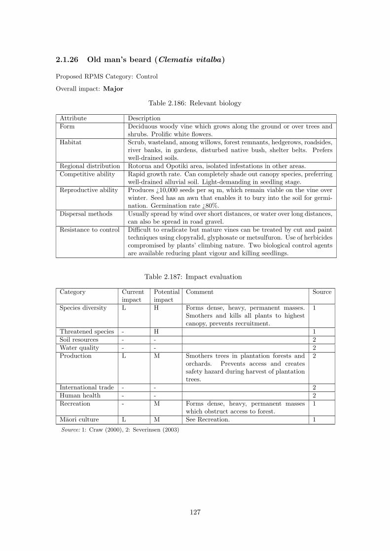
2.1.26 Old man’s beard (Clematis vitalba)
Proposed RPMS Category: Control
Overall impact: Major
Table 2.186: Relevant biology
Attribute DescriptionForm Deciduous woody vine which grows along the ground or over trees and
shrubs. Prolific white flowers.Habitat Scrub, wasteland, among willows, forest remnants, hedgerows, roadsides,
river banks, in gardens, disturbed native bush, shelter belts. Preferswell-drained soils.
Regional distribution Rotorua and Opotiki area, isolated infestations in other areas.Competitive ability Rapid growth rate. Can completely shade out canopy species, preferring
well-drained alluvial soil. Light-demanding in seedling stage.Reproductive ability Produces ¿10,000 seeds per sq m, which remain viable on the vine over
winter. Seed has an awn that enables it to bury into the soil for germi-nation. Germination rate ¿80%.
Dispersal methods Usually spread by wind over short distances, or water over long distances,can also be spread in road gravel.
Resistance to control Di�cult to eradicate but mature vines can be treated by cut and painttechniques using clopyralid, glyphosate or metsulfuron. Use of herbicidescompromised by plants’ climbing nature. Two biological control agentsare available reducing plant vigour and killing seedlings.
Table 2.187: Impact evaluation
Category Currentimpact
Potentialimpact
Comment Source
Species diversity L H Forms dense, heavy, permanent masses.Smothers and kills all plants to highestcanopy, prevents recruitment.
1
Threatened species - H 1Soil resources - - 2Water quality - - 2Production L M Smothers trees in plantation forests and
orchards. Prevents access and createssafety hazard during harvest of plantationtrees.
2
International trade - - 2Human health - - 2Recreation - M Forms dense, heavy, permanent masses
which obstruct access to forest.1
Maori culture L M See Recreation. 1Source: 1: Craw (2000), 2: Severinsen (2003)
127

Old man’s beard CBA results
The following are results for cost-benefit analyses for four scenarios, no regional RPMS control,RPMS control as an Exclusion Pest, RPMS control as a Control Pest, and RPMS control as anAdvisory Pest. For the purposes of the CBA calculations, the pest is assumed to continue expandingwith no regional RPMS control, its spread is assumed to be near-arrested under Advisory Controlbut not reduced, and it is assumed to be successfully reduced to the expected smaller extent whenlisted as a Control Pest, more so as an Exclusion pest.
Table 2.188: Old man’s beard CBA results for four RPMS scenarios, presented as netpresent value (NPV, $) over 50 years. The expenditure refers to regional expenditureunder the RPMS. Minimum and maximum values are in brackets beneath average values.
Scenario Pest impacts Control benefit Expenditure Net benefitNo RPMS 472,264 0 0 -472,264
(129,825–1,352,364) (-129,825 – -1,352,364)
Exclusion Pest 1,524 470,740 7,252,637 -6,781,897(386–2,464) (129,439–1,349,900) (-7,123,198 – -5,902,737)
Control Pest 4,034 468,230 284,062 184,168(971–6,905) (128,854–1,345,459) (-155,208 – 1,061,397)
Advisory Pest 2,152 470,112 13,212 456,900(480–3,968) (129,345–1,348,396) (116,133 – 1,335,184)
Table 2.189: Old man’s beard CBA base assumptions.
Base assumptions ValuesCurrent area infested (ha) 120
Total area potentially infested (ha) 135,022 (45,007–225,037)
Years from naturalisation to total area 125Assessment duration (yr) 50
Weighted average impact per hectare of infested land ($/ha) 2.98 (0.7–5.27)
Any benefits provided by the weed 0Discount rate 0.08
Table 2.190: Old man’s beard RPMS Exclusion Pest assumptions.
Exclusion Pest assumptions ValuesYears to achieve objectives 9
Final area infested (ha) 15 (0–30)
Table 2.191: Old man’s beard RPMS Control Pest assumptions.
Control Pest assumptions ValuesYears to achieve objectives 50
Final area infested (ha) 75 (60–90)
Table 2.192: Old man’s beard RPMS Advisory Pest assumptions.
Advisory Pest assumptions ValuesYears to achieve objectives 5
128

Final area infested (ha) 195 (210–180)
Table 2.193: Old man’s beard estimated total annual cost of di↵erent RPMS scenarios(includes inspection, control, monitoring, enforcement, administration etc.). Subsequentyears are assumed to have the same value as the last year listed.
Exclusion Pest Control Pest Advisory PestYear Total Costs Total Costs Total Costs1.00 1,075,000 21,500 1,000
Old man’s beard conclusions
In the absence of regional control, the projected total regional damage in net present value is-$472,264 over the next 50 years (the minimum projected impact is -$129,825).
Managing Old man’s beard as an Exclusion pest has a projected net benefit to the region of -$6,781,897. Since this is negative, this means that this management scenario does not meets therequirements of Section 72(1a) of the Act.
Managing Old man’s beard as a Control pest has a projected net benefit to the region of $184,168.Since this is positive, this means that this management scenario meets the requirements of Section72(1a) of the Act.
Managing Old man’s beard as an Advisory pest has a projected net benefit to the region of$456,900. Since this is positive, this means that this management scenario meets the requirementsof Section 72(1a) of the Act.
The proposed management scenario for Old man’s beard, Control, therefore meets the requirementsof Section 72(1a) of the Act.
129
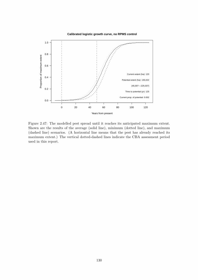
0 20 40 60 80 100 120
0.0
0.2
0.4
0.6
0.8
1.0
Calibrated logistic growth curve, no RPMS control
Years from present
Prop
ortio
n of
max
imum
ext
ent
Current extent (ha): 120
Potential extent (ha): 135,022
(45,007−−225,037)
Time to potential (yr): 125
Current prop. of potential: 0.002
Figure 2.47: The modelled pest spread until it reaches its anticipated maximum extent.Shown are the results of the average (solid line), minimum (dotted line), and maximum(dashed line) scenarios. (A horizontal line means that the pest has already reached itsmaximum extent.) The vertical dotted-dashed lines indicate the CBA assessment periodused in this report.
130

●●
●●
●●
●●
●●
●●
●●
●●
●●
●●
●●
●●
●●
●●
●●
●●
●●
●●
●●
●●
●
●
●
●
●
●
●
●
●
●
●
010
2030
4050
050100
150
200
250
300
350
Popu
latio
n gr
owth
, no
RPM
S co
ntro
l
Year
s fro
m p
rese
nt
Proportion of initial area
●●
●●
●●
●●
●●
●●
●●
●●
●●
●●
●●
●●
●●
●●
●●
●●
●●
●●
●●
●●
●●
●●
●●
●●
●●
●
010
2030
4050
050100
150
200
250
300
350
Dis
coun
ted
grow
th
Year
s fro
m p
rese
nt
Discounted annual cost
Dis
coun
t rat
e: 0
.08
Tota
l mul
tiplie
r: 12
3.27
(105−−
176)
(a)
●
●
●
●
●
●
●
●
●
●
02
46
8
0.0
0.2
0.4
0.6
0.8
1.0
Popu
latio
n gr
owth
, exc
lusi
on c
ontro
l
Year
s fro
m p
rese
ntProportion of initial area
●
●
●
●
●
●
●
●
●
●
02
46
8
0.0
0.2
0.4
0.6
0.8
1.0
Dis
coun
ted
grow
th, e
xclu
sion
con
trol
Year
s of
con
trol
Discounted annual cost
(b)
●●
●●
●●
●●
●●
●●
●●
●●
●●
●●
●●
●●
●●
●●
●●
●●
●●
●●
●●
●●
●●
●●
●●
●●
●●
●
010
2030
4050
0.0
0.2
0.4
0.6
0.8
1.0
Popu
latio
n gr
owth
, con
trol c
ontro
l
Year
s fro
m p
rese
nt
Proportion of initial area
●
●
●
●
●
●
●
●
●
●
●
●
●
●
●
●●
●●
●●
●●
●●
●●
●●
●●
●●
●●
●●
●●
●●
●●
●●
●●
●●
●●
010
2030
4050
0.0
0.2
0.4
0.6
0.8
1.0
Dis
coun
ted
grow
th, c
ontro
l con
trol
Year
s of
con
trol
Discounted annual cost
(c)
●
●
●
●
●
●
01
23
45
0.0
0.5
1.0
1.5
Popu
latio
n gr
owth
, adv
isor
y co
ntro
l
Year
s fro
m p
rese
nt
Proportion of initial area
●
●
●●
●●
01
23
45
0.0
0.2
0.4
0.6
0.8
1.0
Dis
coun
ted
grow
th, a
dvis
ory
cont
rol
Year
s of
con
trol
Discounted annual cost
(d)
Fig
ure
2.48
:T
hem
odel
led
popu
lati
onch
ange
sov
erth
eC
BA
asse
ssm
ent
peri
odfo
r(a
)no
regi
onal
cont
rol,
(b)
Exc
lusi
onPes
tco
ntro
l,(c
)C
ontr
olPes
tco
ntro
l,an
d(d
)A
dvis
ory
Pes
tco
ntro
l.T
heup
per
grap
hssh
owth
epo
pula
tion
chan
ges,
and
the
low
ergr
aphs
show
the
disc
ount
ing
ofas
soci
ated
impa
cts
each
year
(im
pact
sin
the
futu
rear
eof
less
valu
eec
onom
ical
lyth
anim
pact
sof
the
sam
esi
zeno
w).
131

2.1.27 Pampas (Cortaderia selloana, C. jubata and cultivars)
Proposed RPMS Category: Advisory
Overall impact: Moderate
Table 2.194: Relevant biology
Attribute DescriptionForm A tall tussock grass (to 4 m tall) with sharp leaves mostly developing
from the base. Purple pampas has a large purple plume whereas incommon pampas the flower plume is yellow.
Habitat Distributed from subtropical to temperate regions. Prefers disturbedareas like roadside banks, slip faces, and river banks. Common in forestryblocks.
Regional distribution Widespread across region.Competitive ability A major problem in forestry areas. The root system of a single plant
can occupy as much as 103 cubic m of soil.Reproductive ability Up to 100,000 seeds can be produced per flower head.Dispersal methods Seed dispersed primarily by wind (reputedly 10-25 km) however, gravel,
vehicles and animals can also carry seed.Resistance to control Can be controlled using herbicides but is di�cult and repeat applications
are often necessary. Size of mature plants makes mechanical removaldi�cult. Sometimes grazed by stock.
Benefits Used as hedges, windbreaks on farms
Table 2.195: Impact evaluation
Category Currentimpact
Potentialimpact
Comment Source
Species diversity M H Colonises sprayed, burnt, disturbed sitesand quickly becomes very dense. Replacesnative ground covers, shrubs, ferns. Pro-vides habitat for possums and rats.
1
Threatened species L M 1Soil resources - - 2Water quality - - 2Production M M Problem in young plantation forests,
quickly becomes very dense. Build-up ofdead leaves, leaf bases and flowering stalkscreates a significant fire hazard.
1
International trade L M Seed can contaminate kiwifruit and leadto entire crop being rejected for export.
3
Human health L L Sharp leaves can cut skin. 4Recreation M M Forms dense patches which restrict access. 1Maori culture M M See Recreation. 1Source: 1: Craw (2000), 2: Severinsen (2003), 3: Mather (2009), 4: Department of Conservation (1997a)
132

Pampas CBA results
The following are results for cost-benefit analyses for four scenarios, no regional RPMS control,RPMS control as an Exclusion Pest, RPMS control as a Control Pest, and RPMS control as anAdvisory Pest. For the purposes of the CBA calculations, the pest is assumed to continue expandingwith no regional RPMS control, its spread is assumed to be near-arrested under Advisory Controlbut not reduced, and it is assumed to be successfully reduced to the expected smaller extent whenlisted as a Control Pest, more so as an Exclusion pest.
Table 2.196: Pampas CBA results for four RPMS scenarios, presented as net present value(NPV, $) over 50 years. The expenditure refers to regional expenditure under the RPMS.Minimum and maximum values are in brackets beneath average values.
Scenario Pest impacts Control benefit Expenditure Net benefitNo RPMS 53,984,513 0 0 -53,984,513
(13,745,734–171,093,381) (-13,745,734 – -171,093,381)
Exclusion Pest 3,742,891 50,241,622 236,132,363 -185,890,741(1,375,703–5,690,778) (12,370,031–165,402,603) (-223,762,332 – -70,729,760)
Control Pest 9,907,746 44,076,767 13,212,163 30,864,604(3,461,847–15,945,199) (10,283,887–155,148,182) (-2,928,276 – 141,936,019)
Advisory Pest 4,590,574 49,393,939 66,061 49,327,878(1,712,186–6,857,469) (12,033,548–164,235,912) (11,967,487 – 164,169,851)
Table 2.197: Pampas CBA base assumptions.
Base assumptions ValuesCurrent area infested (ha) 6,000
Total area potentially infested (ha) 178,639 (59,558–297,720)
Years from naturalisation to total area 75Assessment duration (yr) 50
Weighted average impact per hectare of infested land ($/ha) 146.48 (49.63–243.33)
Any benefits provided by the weed 1Discount rate 0.08
Table 2.198: Pampas RPMS Exclusion Pest assumptions.
Exclusion Pest assumptions ValuesYears to achieve objectives 9
Final area infested (ha) 750 (0–1,500)
Table 2.199: Pampas RPMS Control Pest assumptions.
Control Pest assumptions ValuesYears to achieve objectives 50
Final area infested (ha) 3,750 (3,000–4,500)
Table 2.200: Pampas RPMS Advisory Pest assumptions.
Advisory Pest assumptions ValuesYears to achieve objectives 5
Final area infested (ha) 7,500 (6,000–9,000)
133

Table 2.201: Pampas estimated total annual cost of di↵erent RPMS scenarios (includesinspection, control, monitoring, enforcement, administration etc.). Subsequent years areassumed to have the same value as the last year listed.
Exclusion Pest Control Pest Advisory PestYear Total Costs Total Costs Total Costs1.00 35,000,000 1,000,000 5,000
Pampas conclusions
In the absence of regional control, the projected total regional damage in net present value is-$53,984,513 over the next 50 years (the minimum projected impact is -$13,745,734).
Managing Pampas as an Exclusion pest has a projected net benefit to the region of -$185,890,741.Since this is negative, this means that this management scenario does not meets the requirementsof Section 72(1a) of the Act.
Managing Pampas as a Control pest has a projected net benefit to the region of $30,864,604. Sincethis is positive, this means that this management scenario meets the requirements of Section 72(1a)of the Act.
Managing Pampas as an Advisory pest has a projected net benefit to the region of $49,327,878.Since this is positive, this means that this management scenario meets the requirements of Section72(1a) of the Act.
The proposed management scenario for Pampas, Advisory, therefore meets the requirements ofSection 72(1a) of the Act.
134

−20 0 20 40 60
0.0
0.2
0.4
0.6
0.8
1.0
Calibrated logistic growth curve, no RPMS control
Years from present
Prop
ortio
n of
max
imum
ext
ent
Current extent (ha): 6,000
Potential extent (ha): 178,639
(59,558−−297,720)
Time to potential (yr): 75
Current prop. of potential: 0.06
Figure 2.49: The modelled pest spread until it reaches its anticipated maximum extent.Shown are the results of the average (solid line), minimum (dotted line), and maximum(dashed line) scenarios. (A horizontal line means that the pest has already reached itsmaximum extent.) The vertical dotted-dashed lines indicate the CBA assessment periodused in this report.
135

●●
●●
●●
●●
●●
●●
●●
●●
●●
●●
●●
●●
●●
●●
●●
●●
●●
●●
●●
●●
●●
●●
●●
●●
●●
●
010
2030
4050
01020304050
Popu
latio
n gr
owth
, no
RPM
S co
ntro
l
Year
s fro
m p
rese
nt
Proportion of initial area
●●
●●
●●
●●
●●
●●
●●
●●
●●
●●
●●
●●
●●
●●
●●
●●
●●
●●
●●
●●
●●
●●
●●
●●
●●
●
010
2030
4050
01020304050
Dis
coun
ted
grow
th
Year
s fro
m p
rese
nt
Discounted annual cost
Dis
coun
t rat
e: 0
.08
Tota
l mul
tiplie
r: 61
.33
(46−−1
17)
(a)
●
●
●
●
●
●
●
●
●
●
02
46
8
0.0
0.2
0.4
0.6
0.8
1.0
Popu
latio
n gr
owth
, exc
lusi
on c
ontro
l
Year
s fro
m p
rese
ntProportion of initial area
●
●
●
●
●
●
●
●
●
●
02
46
8
0.0
0.2
0.4
0.6
0.8
1.0
Dis
coun
ted
grow
th, e
xclu
sion
con
trol
Year
s of
con
trol
Discounted annual cost
(b)
●●
●●
●●
●●
●●
●●
●●
●●
●●
●●
●●
●●
●●
●●
●●
●●
●●
●●
●●
●●
●●
●●
●●
●●
●●
●
010
2030
4050
0.0
0.2
0.4
0.6
0.8
1.0
Popu
latio
n gr
owth
, con
trol c
ontro
l
Year
s fro
m p
rese
nt
Proportion of initial area
●
●
●
●
●
●
●
●
●
●
●
●
●
●
●
●●
●●
●●
●●
●●
●●
●●
●●
●●
●●
●●
●●
●●
●●
●●
●●
●●
●●
010
2030
4050
0.0
0.2
0.4
0.6
0.8
1.0
Dis
coun
ted
grow
th, c
ontro
l con
trol
Year
s of
con
trol
Discounted annual cost
(c)
●
●
●
●
●
●
01
23
45
0.0
0.2
0.4
0.6
0.8
1.0
Popu
latio
n gr
owth
, adv
isor
y co
ntro
l
Year
s fro
m p
rese
nt
Proportion of initial area
●
●
●
●
●
●
01
23
45
0.0
0.2
0.4
0.6
0.8
1.0
Dis
coun
ted
grow
th, a
dvis
ory
cont
rol
Year
s of
con
trol
Discounted annual cost
(d)
Fig
ure
2.50
:T
hem
odel
led
popu
lati
onch
ange
sov
erth
eC
BA
asse
ssm
ent
peri
odfo
r(a
)no
regi
onal
cont
rol,
(b)
Exc
lusi
onPes
tco
ntro
l,(c
)C
ontr
olPes
tco
ntro
l,an
d(d
)A
dvis
ory
Pes
tco
ntro
l.T
heup
per
grap
hssh
owth
epo
pula
tion
chan
ges,
and
the
low
ergr
aphs
show
the
disc
ount
ing
ofas
soci
ated
impa
cts
each
year
(im
pact
sin
the
futu
rear
eof
less
valu
eec
onom
ical
lyth
anim
pact
sof
the
sam
esi
zeno
w).
136

2.1.28 Privet (Ligustrum lucidum, L. sinense)
Proposed RPMS Category: Advisory
Overall impact: Moderate
Table 2.202: Relevant biology
Attribute DescriptionForm Medium sized evergreen tree growing up to 10 m tall (tree privet). Ev-
ergreen or semi-deciduous shrub as small tree up to 5 m tall (Chineseprivet).
Habitat Widely grown as hedging plant, also occurs in lowland and coastal forest,mostly remnants and shrub land. Urban areas, disturbed sites, roadsidebanks, waste areas.
Regional distribution Widespread across region.Competitive ability Tree privet is shade tolerant and competitive on a wide range of soils.
Chinese privet is also shade tolerant (probably also shade requiring).Fire intolerant.
Reproductive ability Both species produce 100,000-10,000,000 seeds per bush or tree.Dispersal methods Seed dispersed by birds.Resistance to control Adequately controlled by cutting and painting with metsulfuron, but
this can possibly damage surrounding areas.
Table 2.203: Impact evaluation
Category Currentimpact
Potentialimpact
Comment Source
Species diversity M H Dense stands prevent recruitment. Dis-places vulnerable shrub species. Poi-sonous berries may possibly impact on na-tive fauna, esp. insects.
1, 2
Threatened species L L 1, 2Soil resources - - 3Water quality - - 3Production L L Forms dense stands. 2, 4International trade - - 3Human health M M Berries and leaves are poisonous. There is
no convincing evidence that pollen a↵ectsasthma and hay fever although many peo-ple believe this.
1, 2
Recreation L L Forms dense stands which restrict access. 1, 2Maori culture L M See Recreation. 3Source: 1: Craw (2000), 2: Environment Bay of Plenty (2005g), 3: Severinsen (2003), 4: Environment
Bay of Plenty (2004a)
137

Privet CBA results
The following are results for cost-benefit analyses for four scenarios, no regional RPMS control,RPMS control as an Exclusion Pest, RPMS control as a Control Pest, and RPMS control as anAdvisory Pest. For the purposes of the CBA calculations, the pest is assumed to continue expandingwith no regional RPMS control, its spread is assumed to be near-arrested under Advisory Controlbut not reduced, and it is assumed to be successfully reduced to the expected smaller extent whenlisted as a Control Pest, more so as an Exclusion pest.
Table 2.204: Privet CBA results for four RPMS scenarios, presented as net present value(NPV, $) over 50 years. The expenditure refers to regional expenditure under the RPMS.Minimum and maximum values are in brackets beneath average values.
Scenario Pest impacts Control benefit Expenditure Net benefitNo RPMS 6,055,811 0 0 -6,055,811
(1,405,216–25,388,392) (-1,405,216 – -25,388,392)
Exclusion Pest 249,520 5,806,291 472,264,726 -466,458,435(72,095–395,928) (1,333,121–24,992,464) (-470,931,605 – -447,272,262)
Control Pest 660,500 5,395,311 13,212,163 -7,816,852(181,422–1,109,364) (1,223,794–24,279,028) (-11,988,369 – 11,066,865)
Advisory Pest 306,031 5,749,780 132,122 5,617,658(89,729–477,098) (1,315,487–24,911,294) (1,183,365 – 24,779,172)
Table 2.205: Privet CBA base assumptions.
Base assumptions ValuesCurrent area infested (ha) 6,000
Total area potentially infested (ha) 106,584 (36,487–176,682)
Years from naturalisation to total area 25Assessment duration (yr) 50
Weighted average impact per hectare of infested land ($/ha) 9.77 (2.6–16.93)
Any benefits provided by the weed 0Discount rate 0.08
Table 2.206: Privet RPMS Exclusion Pest assumptions.
Exclusion Pest assumptions ValuesYears to achieve objectives 9
Final area infested (ha) 750 (0–1,500)
Table 2.207: Privet RPMS Control Pest assumptions.
Control Pest assumptions ValuesYears to achieve objectives 50
Final area infested (ha) 3,750 (3,000–4,500)
Table 2.208: Privet RPMS Advisory Pest assumptions.
Advisory Pest assumptions ValuesYears to achieve objectives 5
Final area infested (ha) 7,500 (6,000–9,000)
138

Table 2.209: Privet estimated total annual cost of di↵erent RPMS scenarios (includesinspection, control, monitoring, enforcement, administration etc.). Subsequent years areassumed to have the same value as the last year listed.
Exclusion Pest Control Pest Advisory PestYear Total Costs Total Costs Total Costs1.00 70,000,000 1,000,000 10,000
Privet conclusions
In the absence of regional control, the projected total regional damage in net present value is-$6,055,811 over the next 50 years (the minimum projected impact is -$1,405,216).
Managing Privet as an Exclusion pest has a projected net benefit to the region of -$466,458,435.Since this is negative, this means that this management scenario does not meets the requirementsof Section 72(1a) of the Act.
Managing Privet as a Control pest has a projected net benefit to the region of -$7,816,852. Sincethis is negative, this means that this management scenario does not meet the requirements ofSection 72(1a) of the Act.
Managing Privet as an Advisory pest has a projected net benefit to the region of $5,617,658. Sincethis is positive, this means that this management scenario meets the requirements of Section 72(1a)of the Act.
The proposed management scenario for Privet, Advisory, therefore meets the requirements ofSection 72(1a) of the Act.
139
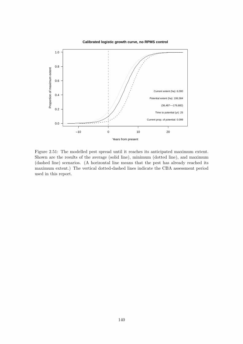
−10 0 10 20
0.0
0.2
0.4
0.6
0.8
1.0
Calibrated logistic growth curve, no RPMS control
Years from present
Prop
ortio
n of
max
imum
ext
ent
Current extent (ha): 6,000
Potential extent (ha): 106,584
(36,487−−176,682)
Time to potential (yr): 25
Current prop. of potential: 0.099
Figure 2.51: The modelled pest spread until it reaches its anticipated maximum extent.Shown are the results of the average (solid line), minimum (dotted line), and maximum(dashed line) scenarios. (A horizontal line means that the pest has already reached itsmaximum extent.) The vertical dotted-dashed lines indicate the CBA assessment periodused in this report.
140

●●
●
●
●
●
●
●
●
●●
●●
●●
●●
●●
●●
●●
●●
●●
●●
●●
●●
●●
●●
●●
●●
●●
●●
●●
●●
●●
010
2030
4050
051015202530
Popu
latio
n gr
owth
, no
RPM
S co
ntro
l
Year
s fro
m p
rese
nt
Proportion of initial area
●●
●●
●●
●●
●●
●●
●●
●●
●●
●●
●●
●●
●●
●●
●●
●●
●●
●●
●●
●●
●●
●●
●●
●●
●●
●
010
2030
4050
051015202530
Dis
coun
ted
grow
th
Year
s fro
m p
rese
nt
Discounted annual cost
Dis
coun
t rat
e: 0
.08
Tota
l mul
tiplie
r: 84
.7
(55−−2
12)
(a)
●
●
●
●
●
●
●
●
●
●
02
46
8
0.0
0.2
0.4
0.6
0.8
1.0
Popu
latio
n gr
owth
, exc
lusi
on c
ontro
l
Year
s fro
m p
rese
ntProportion of initial area
●
●
●
●
●
●
●
●
●
●
02
46
8
0.0
0.2
0.4
0.6
0.8
1.0
Dis
coun
ted
grow
th, e
xclu
sion
con
trol
Year
s of
con
trol
Discounted annual cost
(b)
●●
●●
●●
●●
●●
●●
●●
●●
●●
●●
●●
●●
●●
●●
●●
●●
●●
●●
●●
●●
●●
●●
●●
●●
●●
●
010
2030
4050
0.0
0.2
0.4
0.6
0.8
1.0
Popu
latio
n gr
owth
, con
trol c
ontro
l
Year
s fro
m p
rese
nt
Proportion of initial area
●
●
●
●
●
●
●
●
●
●
●
●
●
●
●
●●
●●
●●
●●
●●
●●
●●
●●
●●
●●
●●
●●
●●
●●
●●
●●
●●
●●
010
2030
4050
0.0
0.2
0.4
0.6
0.8
1.0
Dis
coun
ted
grow
th, c
ontro
l con
trol
Year
s of
con
trol
Discounted annual cost
(c)
●
●
●
●
●
●
01
23
45
0.0
0.2
0.4
0.6
0.8
1.0
Popu
latio
n gr
owth
, adv
isor
y co
ntro
l
Year
s fro
m p
rese
nt
Proportion of initial area
●
●
●
●
●
●
01
23
45
0.0
0.2
0.4
0.6
0.8
1.0
Dis
coun
ted
grow
th, a
dvis
ory
cont
rol
Year
s of
con
trol
Discounted annual cost
(d)
Fig
ure
2.52
:T
hem
odel
led
popu
lati
onch
ange
sov
erth
eC
BA
asse
ssm
ent
peri
odfo
r(a
)no
regi
onal
cont
rol,
(b)
Exc
lusi
onPes
tco
ntro
l,(c
)C
ontr
olPes
tco
ntro
l,an
d(d
)A
dvis
ory
Pes
tco
ntro
l.T
heup
per
grap
hssh
owth
epo
pula
tion
chan
ges,
and
the
low
ergr
aphs
show
the
disc
ount
ing
ofas
soci
ated
impa
cts
each
year
(im
pact
sin
the
futu
rear
eof
less
valu
eec
onom
ical
lyth
anim
pact
sof
the
sam
esi
zeno
w).
141

2.1.29 Ragwort (Senecio jacobaea)
Proposed RPMS Category: Advisory
Overall impact: Moderate
Table 2.210: Relevant biology
Attribute DescriptionForm An erect biennial or perennial herb, usually growing to 45-60 cm. Single
or several stems arise from a crown, with dark green leaves. Flowers arebright yellow and clustered at the end of the branches.
Habitat Waste places and pasture, also riverbeds, open forest, swamps. Occursin humid temperate regions with annual rainfall greater than 750 mm.Tolerates frost.
Regional distribution Widespread throughout region. Most problematic in dairying districtsbecause of higher rainfall and unpalatable to cattle.
Competitive ability Establishment is poor in pasture but good in disturbed soil. Earlygrowth is slow and seedling mortality high.
Reproductive ability Can flower all year around. A well developed plant may produce 250,000seeds per year of which 80% may be viable. Seed can be viable for atleast 8 years and germinate when brought to the surface.
Dispersal methods Wind is main method of seed spread. New Zealand study showed bulkof seed fell to ground within 5 m of the parent plant and virtually nonewas blown more than 37 m.
Resistance to control Can be controlled grazing, mowing, grubbing, and herbicides, but canbecome resistant to chemical control as a result of poor application.Grubbing and spraying can produce multi-headed plants. Plants mayregenerate after flowering. Ragwort flea beetle is widespread throughoutthe region and appears to be achieving reasonable control.
Table 2.211: Impact evaluation
Category Currentimpact
Potentialimpact
Comment Source
Species diversity - - 1Threatened species - - 1Soil resources - - 1Water quality - - 1Production M M Forms dense stands in disturbed and
grazed areas. Alkaloids present are toxicto horses, cattle, deer.
2, 3, 4,5
International trade - L Prohibited seed of nil tolerance in Aus-tralia.
6
Human health L L Can cause skin irritation and allergieswhen handed extensively.
7
Recreation - - 1Maori culture - - 1Source: 1: Severinsen (2003), 2: Craw (2000), 3: Roy et al. (2004), 4: Environment Bay of Plenty (2005h),
5: Anon. (2007e), 6: Anon. (2009k), 7: Gourlay (2009)
142

Ragwort CBA results
The following are results for cost-benefit analyses for four scenarios, no regional RPMS control,RPMS control as an Exclusion Pest, RPMS control as a Control Pest, and RPMS control as anAdvisory Pest. For the purposes of the CBA calculations, the pest is assumed to continue expandingwith no regional RPMS control, its spread is assumed to be near-arrested under Advisory Controlbut not reduced, and it is assumed to be successfully reduced to the expected smaller extent whenlisted as a Control Pest, more so as an Exclusion pest.
Table 2.212: Ragwort CBA results for four RPMS scenarios, presented as net presentvalue (NPV, $) over 50 years. The expenditure refers to regional expenditure under theRPMS. Minimum and maximum values are in brackets beneath average values.
Scenario Pest impacts Control benefit Expenditure Net benefitNo RPMS 5,752,613,251 0 0 -5,752,613,251
(3,031,907,182–3,524,596,474) (-3,031,907,182 – -3,524,596,474)
Exclusion Pest 285,465,812 5,467,147,439 27,492,554 5,439,654,885(99,830,471–438,326,138) (2,932,076,711–3,086,270,336) (2,904,584,157 – 3,058,777,782)
Control Pest 755,651,959 4,996,961,292 1,076,791 4,995,884,501(251,215,426–1,228,161,911) (2,780,691,756–2,296,434,563) (2,779,614,965 – 2,295,357,772)
Advisory Pest 314,847,652 5,437,765,599 13,212 5,437,752,387(101,506,066–528,189,237) (2,930,401,116–2,996,407,237) (2,930,387,904 – 2,996,394,025)
Table 2.213: Ragwort CBA base assumptions.
Base assumptions ValuesCurrent area infested (ha) 253,856
Total area potentially infested (ha) 62,322 (22,295–102,349)
Years from naturalisation to total area 50Assessment duration (yr) 50
Weighted average impact per hectare of infested land ($/ha) 264.06 (85.13–442.98)
Any benefits provided by the weed 0Discount rate 0.08
Table 2.214: Ragwort RPMS Exclusion Pest assumptions.
Exclusion Pest assumptions ValuesYears to achieve objectives 9
Final area infested (ha) 31,732 (0–63,464)
Table 2.215: Ragwort RPMS Control Pest assumptions.
Control Pest assumptions ValuesYears to achieve objectives 50
Final area infested (ha) 158,660 (126,928–190,392)
Table 2.216: Ragwort RPMS Advisory Pest assumptions.
Advisory Pest assumptions ValuesYears to achieve objectives 5
Final area infested (ha) 253,856 (253,856–253,856)
143

Table 2.217: Ragwort estimated total annual cost of di↵erent RPMS scenarios (includesinspection, control, monitoring, enforcement, administration etc.). Subsequent years areassumed to have the same value as the last year listed.
Exclusion Pest Control Pest Advisory PestYear Total Costs Total Costs Total Costs1.00 4,075,000 81,500 1,000
Ragwort conclusions
In the absence of regional control, the projected total regional damage in net present value is-$5,752,613,251 over the next 50 years (the minimum projected impact is -$3,031,907,182).
Managing Ragwort as an Exclusion pest has a projected net benefit to the region of $5,439,654,885.Since this is positive, this means that this management scenario meets the requirements of Section72(1a) of the Act.
Managing Ragwort as a Control pest has a projected net benefit to the region of $4,995,884,501.Since this is positive, this means that this management scenario meets the requirements of Section72(1a) of the Act.
Managing Ragwort as an Advisory pest has a projected net benefit to the region of $5,437,752,387.Since this is positive, this means that this management scenario meets the requirements of Section72(1a) of the Act.
The proposed management scenario for Ragwort, Advisory, therefore meets the requirements ofSection 72(1a) of the Act.
144

0 10 20 30 40 50
0.0
0.2
0.4
0.6
0.8
1.0
Calibrated logistic growth curve
Years from present
Prop
ortio
n of
max
imum
ext
ent
Current extent (ha): 253,856
Potential extent (ha): 62,322
(22,295−−102,349)
Time to potential (yr): 50
Current prop. of potential: 6.933
Figure 2.53: The modelled pest spread until it reaches its anticipated maximum extent.Shown are the results of the average (solid line), minimum (dotted line), and maximum(dashed line) scenarios. (A horizontal line means that the pest has already reached itsmaximum extent.) The vertical dotted-dashed lines indicate the CBA assessment periodused in this report.
145

● 010
2030
4050
1.0
1.5
2.0
2.5
Popu
latio
n gr
owth
, no
RPM
S co
ntro
l
Year
s fro
m p
rese
nt
Proportion of initial area
●
●
●
●
●
●
●
●
●
●
●
●
●
●
●
●
●
●
●
●
●
●
●
●
●
●
●
●
●
●
●●
●●
●●
●●
●●
●●
●●
●●
●●
●●
●
010
2030
4050
0.0
0.5
1.0
1.5
2.0
2.5
Dis
coun
ted
grow
th
Year
s fro
m p
rese
nt
Discounted annual cost
Dis
coun
t rat
e: 0
.08
Tota
l mul
tiplie
r: 85
.82
(140−−
31)
(a)
●
●
●
●
●
●
●
●
●
●
02
46
8
0.0
0.2
0.4
0.6
0.8
1.0
Popu
latio
n gr
owth
, exc
lusi
on c
ontro
l
Year
s fro
m p
rese
ntProportion of initial area
●
●
●
●
●
●
●
●
●
●
02
46
8
0.0
0.2
0.4
0.6
0.8
1.0
Dis
coun
ted
grow
th, e
xclu
sion
con
trol
Year
s of
con
trol
Discounted annual cost
(b)
●●
●●
●●
●●
●●
●●
●●
●●
●●
●●
●●
●●
●●
●●
●●
●●
●●
●●
●●
●●
●●
●●
●●
●●
●●
●
010
2030
4050
0.0
0.2
0.4
0.6
0.8
1.0
Popu
latio
n gr
owth
, con
trol c
ontro
l
Year
s fro
m p
rese
nt
Proportion of initial area
●
●
●
●
●
●
●
●
●
●
●
●
●
●
●
●●
●●
●●
●●
●●
●●
●●
●●
●●
●●
●●
●●
●●
●●
●●
●●
●●
●●
010
2030
4050
0.0
0.2
0.4
0.6
0.8
1.0
Dis
coun
ted
grow
th, c
ontro
l con
trol
Year
s of
con
trol
Discounted annual cost
(c)
●●
●●
●●
01
23
45
0.0
0.2
0.4
0.6
0.8
1.0
Popu
latio
n gr
owth
, adv
isor
y co
ntro
l
Year
s fro
m p
rese
nt
Proportion of initial area
●
●
●
●
●
●
01
23
45
0.0
0.2
0.4
0.6
0.8
1.0
Dis
coun
ted
grow
th, a
dvis
ory
cont
rol
Year
s of
con
trol
Discounted annual cost
(d)
Fig
ure
2.54
:T
hem
odel
led
popu
lati
onch
ange
sov
erth
eC
BA
asse
ssm
ent
peri
odfo
r(a
)no
regi
onal
cont
rol,
(b)
Exc
lusi
onPes
tco
ntro
l,(c
)C
ontr
olPes
tco
ntro
l,an
d(d
)A
dvis
ory
Pes
tco
ntro
l.T
heup
per
grap
hssh
owth
epo
pula
tion
chan
ges,
and
the
low
ergr
aphs
show
the
disc
ount
ing
ofas
soci
ated
impa
cts
each
year
(im
pact
sin
the
futu
rear
eof
less
valu
eec
onom
ical
lyth
anim
pact
sof
the
sam
esi
zeno
w).
146

2.1.30 Royal fern (Osmunda regalis)
Proposed RPMS Category: Control
Overall impact: Major
Table 2.218: Relevant biology
Attribute DescriptionForm Rhizomatous fern with thick erect trunks to 1.5 m tall. Fronds to 3 m
long. Fertile fronds bearing sterile pinnae at the base and much reducedfertile pinnae at the tip of the frond.
Habitat Wetlands.Regional distribution Matakana Island, Kaituna Wetland, Matata and Rotorua areas.Competitive ability Can exclude other wetland species.Reproductive ability Produces fertile spores.Dispersal methods Disperses by spores.Resistance to control Unknown.
Table 2.219: Impact evaluation
Category Currentimpact
Potentialimpact
Comment Source
Species diversity H H Competes with native species for space inspecialised niches, one of very few weedsof bogs.
1, 2
Threatened species H H Impacting on rare ferns on Matakana Is-land (e.g., Cyclosorus sp.).
1, 2
Soil resources - - 3Water quality - - 3Production - - 3International trade - - 3Human health - - 3Recreation - - 3Maori culture - L Could obstruct access to cultural sites
(e.g. waahi tapu, urupa).1
Source: 1: Craw (2000), 2: Stahl (2009), 3: Severinsen (2003)
147
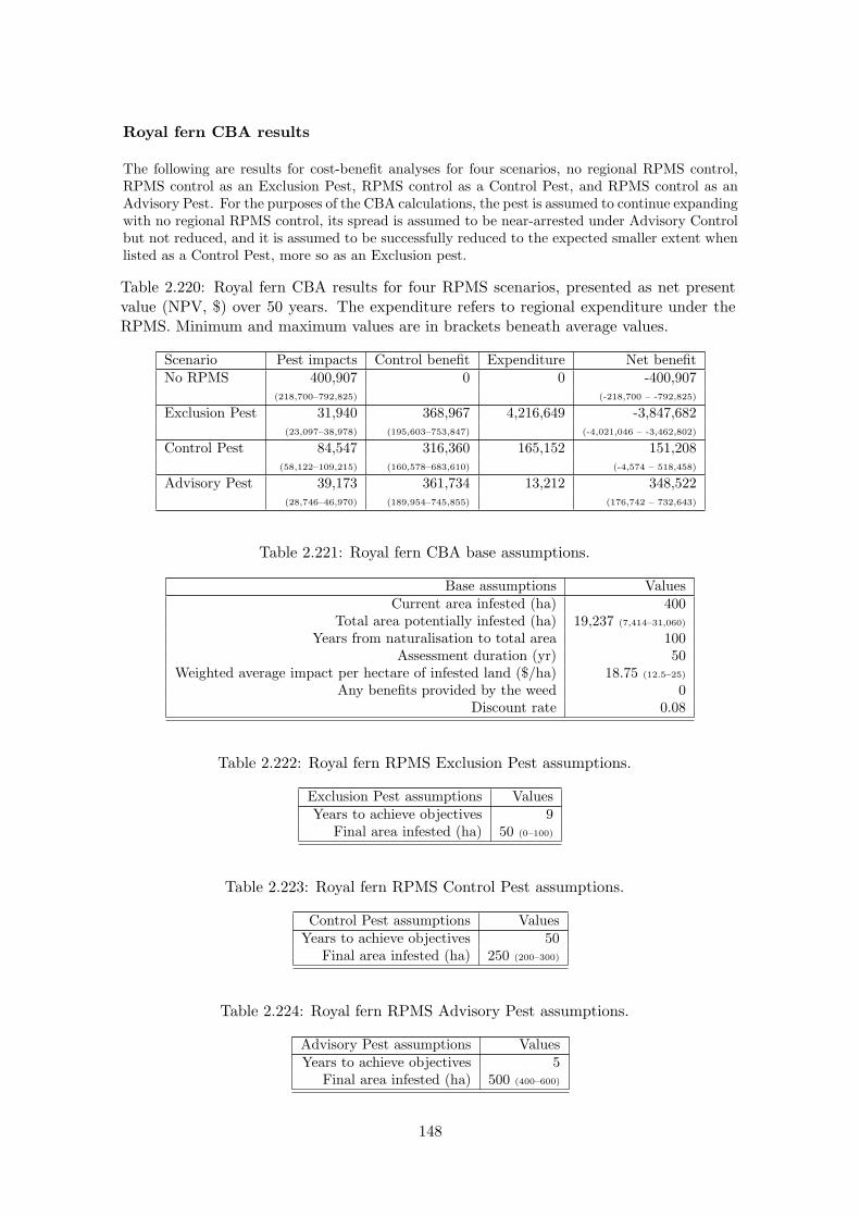
Royal fern CBA results
The following are results for cost-benefit analyses for four scenarios, no regional RPMS control,RPMS control as an Exclusion Pest, RPMS control as a Control Pest, and RPMS control as anAdvisory Pest. For the purposes of the CBA calculations, the pest is assumed to continue expandingwith no regional RPMS control, its spread is assumed to be near-arrested under Advisory Controlbut not reduced, and it is assumed to be successfully reduced to the expected smaller extent whenlisted as a Control Pest, more so as an Exclusion pest.
Table 2.220: Royal fern CBA results for four RPMS scenarios, presented as net presentvalue (NPV, $) over 50 years. The expenditure refers to regional expenditure under theRPMS. Minimum and maximum values are in brackets beneath average values.
Scenario Pest impacts Control benefit Expenditure Net benefitNo RPMS 400,907 0 0 -400,907
(218,700–792,825) (-218,700 – -792,825)
Exclusion Pest 31,940 368,967 4,216,649 -3,847,682(23,097–38,978) (195,603–753,847) (-4,021,046 – -3,462,802)
Control Pest 84,547 316,360 165,152 151,208(58,122–109,215) (160,578–683,610) (-4,574 – 518,458)
Advisory Pest 39,173 361,734 13,212 348,522(28,746–46,970) (189,954–745,855) (176,742 – 732,643)
Table 2.221: Royal fern CBA base assumptions.
Base assumptions ValuesCurrent area infested (ha) 400
Total area potentially infested (ha) 19,237 (7,414–31,060)
Years from naturalisation to total area 100Assessment duration (yr) 50
Weighted average impact per hectare of infested land ($/ha) 18.75 (12.5–25)
Any benefits provided by the weed 0Discount rate 0.08
Table 2.222: Royal fern RPMS Exclusion Pest assumptions.
Exclusion Pest assumptions ValuesYears to achieve objectives 9
Final area infested (ha) 50 (0–100)
Table 2.223: Royal fern RPMS Control Pest assumptions.
Control Pest assumptions ValuesYears to achieve objectives 50
Final area infested (ha) 250 (200–300)
Table 2.224: Royal fern RPMS Advisory Pest assumptions.
Advisory Pest assumptions ValuesYears to achieve objectives 5
Final area infested (ha) 500 (400–600)
148

Table 2.225: Royal fern estimated total annual cost of di↵erent RPMS scenarios (includesinspection, control, monitoring, enforcement, administration etc.). Subsequent years areassumed to have the same value as the last year listed.
Exclusion Pest Control Pest Advisory PestYear Total Costs Total Costs Total Costs1.00 625,000 12,500 1,000
Royal fern conclusions
In the absence of regional control, the projected total regional damage in net present value is-$400,907 over the next 50 years (the minimum projected impact is -$218,700).
Managing Royal fern as an Exclusion pest has a projected net benefit to the region of -$3,847,682.Since this is negative, this means that this management scenario does not meets the requirementsof Section 72(1a) of the Act.
Managing Royal fern as a Control pest has a projected net benefit to the region of $151,208. Sincethis is positive, this means that this management scenario meets the requirements of Section 72(1a)of the Act.
Managing Royal fern as an Advisory pest has a projected net benefit to the region of $348,522.Since this is positive, this means that this management scenario meets the requirements of Section72(1a) of the Act.
The proposed management scenario for Royal fern, Control, therefore meets the requirements ofSection 72(1a) of the Act.
149

−40 −20 0 20 40 60 80 100
0.0
0.2
0.4
0.6
0.8
1.0
Calibrated logistic growth curve, no RPMS control
Years from present
Prop
ortio
n of
max
imum
ext
ent
Current extent (ha): 400
Potential extent (ha): 19,237
(7,414−−31,060)
Time to potential (yr): 100
Current prop. of potential: 0.033
Figure 2.55: The modelled pest spread until it reaches its anticipated maximum extent.Shown are the results of the average (solid line), minimum (dotted line), and maximum(dashed line) scenarios. (A horizontal line means that the pest has already reached itsmaximum extent.) The vertical dotted-dashed lines indicate the CBA assessment periodused in this report.
150

●●
●●
●●
●●
●●
●●
●●
●●
●●
●●
●●
●●
●●
●●
●●
●●
●●
●●
●●
●●
●●
●●
●●
●●
●●
●
010
2030
4050
0102030405060
Popu
latio
n gr
owth
, no
RPM
S co
ntro
l
Year
s fro
m p
rese
nt
Proportion of initial area
●●
●●
●●
●●
●●
●●
●●
●●
●●
●●
●●
●●
●●
●●
●●
●●
●●
●●
●●
●●
●●
●●
●●
●●
●●
●
010
2030
4050
0102030405060
Dis
coun
ted
grow
th
Year
s fro
m p
rese
nt
Discounted annual cost
Dis
coun
t rat
e: 0
.08
Tota
l mul
tiplie
r: 61
.1
(49−−9
5)
(a)
●
●
●
●
●
●
●
●
●
●
02
46
8
0.0
0.2
0.4
0.6
0.8
1.0
Popu
latio
n gr
owth
, exc
lusi
on c
ontro
l
Year
s fro
m p
rese
ntProportion of initial area
●
●
●
●
●
●
●
●
●
●
02
46
8
0.0
0.2
0.4
0.6
0.8
1.0
Dis
coun
ted
grow
th, e
xclu
sion
con
trol
Year
s of
con
trol
Discounted annual cost
(b)
●●
●●
●●
●●
●●
●●
●●
●●
●●
●●
●●
●●
●●
●●
●●
●●
●●
●●
●●
●●
●●
●●
●●
●●
●●
●
010
2030
4050
0.0
0.2
0.4
0.6
0.8
1.0
Popu
latio
n gr
owth
, con
trol c
ontro
l
Year
s fro
m p
rese
nt
Proportion of initial area
●
●
●
●
●
●
●
●
●
●
●
●
●
●
●
●●
●●
●●
●●
●●
●●
●●
●●
●●
●●
●●
●●
●●
●●
●●
●●
●●
●●
010
2030
4050
0.0
0.2
0.4
0.6
0.8
1.0
Dis
coun
ted
grow
th, c
ontro
l con
trol
Year
s of
con
trol
Discounted annual cost
(c)
●
●
●
●
●
●
01
23
45
0.0
0.2
0.4
0.6
0.8
1.0
Popu
latio
n gr
owth
, adv
isor
y co
ntro
l
Year
s fro
m p
rese
nt
Proportion of initial area
●
●
●
●
●
●
01
23
45
0.0
0.2
0.4
0.6
0.8
1.0
Dis
coun
ted
grow
th, a
dvis
ory
cont
rol
Year
s of
con
trol
Discounted annual cost
(d)
Fig
ure
2.56
:T
hem
odel
led
popu
lati
onch
ange
sov
erth
eC
BA
asse
ssm
ent
peri
odfo
r(a
)no
regi
onal
cont
rol,
(b)
Exc
lusi
onPes
tco
ntro
l,(c
)C
ontr
olPes
tco
ntro
l,an
d(d
)A
dvis
ory
Pes
tco
ntro
l.T
heup
per
grap
hssh
owth
epo
pula
tion
chan
ges,
and
the
low
ergr
aphs
show
the
disc
ount
ing
ofas
soci
ated
impa
cts
each
year
(im
pact
sin
the
futu
rear
eof
less
valu
eec
onom
ical
lyth
anim
pact
sof
the
sam
esi
zeno
w).
151

2.1.31 Saltwater paspalum (Paspalum vaginatum)
Proposed RPMS Category: Advisory
Overall impact: Moderate
Table 2.226: Relevant biology
Attribute DescriptionForm Perennial grass that forms dense mats along margins of tidal flats or on
sandy or gravel beaches.Habitat Margins of estuaries and sandy and gravel beaches.Regional distribution Tauranga Harbour, Ohiwa Harbour and other estuaries in the region.Competitive ability Forms dense mats along margins of tidal flats or on sandy gravel beaches.Reproductive ability Does not set viable seed in NZ.Dispersal methods Spread by fragments floating in the water or by cattle grazing. Deliber-
ately planted by humans for erosion control.Resistance to control Unknown.Benefits Prevents erosion in estuaries and along the coast.
Table 2.227: Impact evaluation
Category Currentimpact
Potentialimpact
Comment Source
Species diversity H H Forms dense mats along margins of tidalflats or on sandy gravel beaches. Reducesfeeding and roosting sites for birds, mayalter fish spawning and feeding grounds.
1, 2
Threatened species L H 1Soil resources - - 1Water quality L L May change estuarine hydrology by accu-
mulating sedliment.1
Production - - 1International trade - - 1Human health - - 1Recreation L M Forms dense patches which restrict access
to estuaries.1
Maori culture L M Could destroy and obstruct access tokaimoana (shellfish) gathering areas.
1, 3
Source: 1: QEII (2008), 2: Stahl (2009), 3: Hutchison (2009)
152

Saltwater paspalum CBA results
The following are results for cost-benefit analyses for four scenarios, no regional RPMS control,RPMS control as an Exclusion Pest, RPMS control as a Control Pest, and RPMS control as anAdvisory Pest. For the purposes of the CBA calculations, the pest is assumed to continue expandingwith no regional RPMS control, its spread is assumed to be near-arrested under Advisory Controlbut not reduced, and it is assumed to be successfully reduced to the expected smaller extent whenlisted as a Control Pest, more so as an Exclusion pest.
Table 2.228: Saltwater paspalum CBA results for four RPMS scenarios, presented as netpresent value (NPV, $) over 50 years. The expenditure refers to regional expenditureunder the RPMS. Minimum and maximum values are in brackets beneath average values.
Scenario Pest impacts Control benefit Expenditure Net benefitNo RPMS 21,693 0 0 -21,693
(11,466–47,526) (-11,466 – -47,526)
Exclusion Pest 3,194 18,499 1,349,328 -1,330,829(2,310–3,898) (9,156–43,628) (-1,340,172 – -1,305,700)
Control Pest 8,929 12,764 264,243 -251,479(6,093–11,624) (5,373–35,902) (-258,870 – -228,341)
Advisory Pest 4,154 17,539 13,212 4,327(2,401–6,275) (9,065–41,251) (-4,147 – 28,039)
Table 2.229: Saltwater paspalum CBA base assumptions.
Base assumptions ValuesCurrent area infested (ha) 100
Total area potentially infested (ha) 1,032 (344–1,720)
Years from naturalisation to total area 100Assessment duration (yr) 50
Weighted average impact per hectare of infested land ($/ha) 7.5 (5–10)
Any benefits provided by the weed 1Discount rate 0.08
Table 2.230: Saltwater paspalum RPMS Exclusion Pest assumptions.
Exclusion Pest assumptions ValuesYears to achieve objectives 9
Final area infested (ha) 12.5 (0–25)
Table 2.231: Saltwater paspalum RPMS Control Pest assumptions.
Control Pest assumptions ValuesYears to achieve objectives 50
Final area infested (ha) 85 (75–95)
Table 2.232: Saltwater paspalum RPMS Advisory Pest assumptions.
Advisory Pest assumptions ValuesYears to achieve objectives 5
153
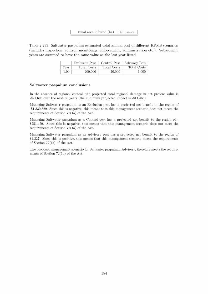
Final area infested (ha) 140 (175–105)
Table 2.233: Saltwater paspalum estimated total annual cost of di↵erent RPMS scenarios(includes inspection, control, monitoring, enforcement, administration etc.). Subsequentyears are assumed to have the same value as the last year listed.
Exclusion Pest Control Pest Advisory PestYear Total Costs Total Costs Total Costs1.00 200,000 20,000 1,000
Saltwater paspalum conclusions
In the absence of regional control, the projected total regional damage in net present value is-$21,693 over the next 50 years (the minimum projected impact is -$11,466).
Managing Saltwater paspalum as an Exclusion pest has a projected net benefit to the region of-$1,330,829. Since this is negative, this means that this management scenario does not meets therequirements of Section 72(1a) of the Act.
Managing Saltwater paspalum as a Control pest has a projected net benefit to the region of -$251,479. Since this is negative, this means that this management scenario does not meet therequirements of Section 72(1a) of the Act.
Managing Saltwater paspalum as an Advisory pest has a projected net benefit to the region of$4,327. Since this is positive, this means that this management scenario meets the requirementsof Section 72(1a) of the Act.
The proposed management scenario for Saltwater paspalum, Advisory, therefore meets the require-ments of Section 72(1a) of the Act.
154

−50 0 50 100
0.0
0.2
0.4
0.6
0.8
1.0
Calibrated logistic growth curve, no RPMS control
Years from present
Prop
ortio
n of
max
imum
ext
ent
Current extent (ha): 100
Potential extent (ha): 1,032
(344−−1,720)
Time to potential (yr): 100
Current prop. of potential: 0.174
Figure 2.57: The modelled pest spread until it reaches its anticipated maximum extent.Shown are the results of the average (solid line), minimum (dotted line), and maximum(dashed line) scenarios. (A horizontal line means that the pest has already reached itsmaximum extent.) The vertical dotted-dashed lines indicate the CBA assessment periodused in this report.
155

●●
●●
●●
●●
●●
●●
●●
●●
●●
●●
●●
●●
●●
●●
●●
●●
●●
●●
●●
●●
●●
●●
●●
●●
●●
●
010
2030
4050
51015
Popu
latio
n gr
owth
, no
RPM
S co
ntro
l
Year
s fro
m p
rese
nt
Proportion of initial area
●●
●●
●●
●●
●●
●●
●●
●●
●●
●●
●●
●●
●●
●●
●●
●●
●●
●●
●●
●●
●●
●●
●●
●●
●●
●
010
2030
4050
051015
Dis
coun
ted
grow
th
Year
s fro
m p
rese
nt
Discounted annual cost
Dis
coun
t rat
e: 0
.08
Tota
l mul
tiplie
r: 28
.92
(23−−4
8)
(a)
●
●
●
●
●
●
●
●
●
●
02
46
8
0.0
0.2
0.4
0.6
0.8
1.0
Popu
latio
n gr
owth
, exc
lusi
on c
ontro
l
Year
s fro
m p
rese
ntProportion of initial area
●
●
●
●
●
●
●
●
●
●
02
46
8
0.0
0.2
0.4
0.6
0.8
1.0
Dis
coun
ted
grow
th, e
xclu
sion
con
trol
Year
s of
con
trol
Discounted annual cost
(b)
●●
●●
●●
●●
●●
●●
●●
●●
●●
●●
●●
●●
●●
●●
●●
●●
●●
●●
●●
●●
●●
●●
●●
●●
●●
●
010
2030
4050
0.0
0.2
0.4
0.6
0.8
1.0
Popu
latio
n gr
owth
, con
trol c
ontro
l
Year
s fro
m p
rese
nt
Proportion of initial area
●
●
●
●
●
●
●
●
●
●
●
●
●
●
●
●●
●●
●●
●●
●●
●●
●●
●●
●●
●●
●●
●●
●●
●●
●●
●●
●●
●●
010
2030
4050
0.0
0.2
0.4
0.6
0.8
1.0
Dis
coun
ted
grow
th, c
ontro
l con
trol
Year
s of
con
trol
Discounted annual cost
(c)
●
●
●
●
●
●
01
23
45
0.0
0.5
1.0
1.5
Popu
latio
n gr
owth
, adv
isor
y co
ntro
l
Year
s fro
m p
rese
nt
Proportion of initial area
●
●●
●●
●
01
23
45
0.0
0.2
0.4
0.6
0.8
1.0
Dis
coun
ted
grow
th, a
dvis
ory
cont
rol
Year
s of
con
trol
Discounted annual cost
(d)
Fig
ure
2.58
:T
hem
odel
led
popu
lati
onch
ange
sov
erth
eC
BA
asse
ssm
ent
peri
odfo
r(a
)no
regi
onal
cont
rol,
(b)
Exc
lusi
onPes
tco
ntro
l,(c
)C
ontr
olPes
tco
ntro
l,an
d(d
)A
dvis
ory
Pes
tco
ntro
l.T
heup
per
grap
hssh
owth
epo
pula
tion
chan
ges,
and
the
low
ergr
aphs
show
the
disc
ount
ing
ofas
soci
ated
impa
cts
each
year
(im
pact
sin
the
futu
rear
eof
less
valu
eec
onom
ical
lyth
anim
pact
sof
the
sam
esi
zeno
w).
156

2.1.32 Senegal tea (Gymnocoronis spilanthoides)
Proposed RPMS Category: Exclusion
Overall impact: Major
Table 2.234: Relevant biology
Attribute DescriptionForm Mat forming perennial aquatic herb with scrambling, floating stems,
which produce roots at nodes. Stems erect when flowering to 1.5 m tall.Habitat Wet marshy soils often spreading out from water margins to form a
floating mat.Regional distribution One site at Welcome Bay.Competitive ability Dominates shorter herbaceous vegetation and floating mats shade out
submerged species.Reproductive ability Few seeds are produced in New Zealand, however seeds are highly fertile.Dispersal methods Spreads by stem fragmentation, humans and machinery. Seeds dispersed
by water movement.Resistance to control Mechanical control unsuccessful as it spreads fragments of the plant.
Can be controlled with herbicides.
Table 2.235: Impact evaluation
Category Currentimpact
Potentialimpact
Comment Source
Species diversity - H Dominates shorter vegetation and floatingmats shade out submerged species.
1, 2, 3
Threatened species - H 1, 2, 3Soil resources - - 4Water quality - H Blocks up waterways. 1, 2, 3Production - - 3International trade - - 4Human health - - 4Recreation - M Dense mats restrict access to waterways
for fishing, swimming, kayaking etc.2, 3
Maori culture - M See Recreation. 5Source: 1: Craw (2000), 2: Anon. (2007f), 3: Anon. (2009h), 4: Severinsen (2003), 5: Stahl (2009)
157

Senegal tea CBA results
Since Senegal tea is currently absent from the region, it is di�cult to accurately quantify the costsand benefits of current and proposed e↵orts to continue to exclude the species. If the species wereto invade this year and spread in the region, without regional control for the next 50 years, thetotal pest impacts over this period in net present value are calculated to be $106,639 ($47,878–$188,615). This can be compared with the calculated net present value of the proposed annualexpenditure on control over this same period of $6,747 (Exclusion pest). Note that this comparisondoes not take into account whether or not the proposed level of expenditure is adequate to havea high probability of excluding the species over this period. Given the broad experience of thebiosecurity sta↵ at Environment Bay of Plenty, we assume that it will be.
The following tables provide the parameters used in this cost-benefit analysis.
Table 2.236: Senegal tea CBA base assumptions.
Base assumptions ValuesCurrent area infested (ha) 0
Total area potentially infested (ha) 4,216 (1,405–7,027)
Years from naturalisation to total area 100Assessment duration (yr) 50
Weighted average impact per hectare of infested land ($/ha) 1 (1–1)
Any benefits provided by the weed 0Discount rate 0.08
Table 2.237: Senegal tea estimated total annual cost of the proposed RPMS scenario(includes inspection, control, monitoring, enforcement, administration etc.). Subsequentyears are assumed to have the same value as the last year listed.
Exclusion PestYear Total Costs1.00 1,000
Senegal tea conclusions
Since the calculated average impact should the species invade is greater than the anticipated expen-diture, and regional establishment is likely in the absence of regional surveillance and preparationsfor rapid response, this management scenario meets the requirements of Section 72(1a) of theAct.
158

2.1.33 Spartina (Spartina anglica, S. alterniflora, S.
“texttimes ”emphtownsendii)
Proposed RPMS Category: Exclusion
Overall impact: Major
Table 2.238: Relevant biology
Attribute DescriptionForm Robust erect perennial growing up to 1 m tall.Habitat Mainly in saline wetlands, especially in estuaries where it forms dense
mats in inter-tidal zones. Prefers deep, soft mud with a sandy loamtexture. Can establish in the tidal ends of streams and rivers.
Regional distribution Tauranga Harbour, Ohiwa Harbour and Maketu estuary.Competitive ability Once established forms dense stands, which may spread at a rate of 2%
per annum.Reproductive ability S. anglica reproduces by seed. S. alterniflora rarely flowers in New
Zealand. S. x townsendii is a sterile hybrid.Dispersal methods Seed and vegetative fragments carried by water. Planted to aid foreshore
protection and stabilize marshes due to its ability to trap sediment. Alsoto assist reclamation of tidal flats.
Resistance to control Well controlled with herbicide.Benefits Prevents erosion at estuary margins.
Table 2.239: Impact evaluation
Category Currentimpact
Potentialimpact
Comment Source
Species diversity M H Traps sediment, raising level above hightide mark, destroys intertidal zone andhabitat. Adventive grasses succeedspartina, creating dry meadows. Immensebiodiversity loss.
1, 2, 3
Threatened species L H 1, 2, 3Soil resources - - 4Water quality M H Can reduce large estuaries and shallow
harbours to thin drains surrounded byrough pasture.
2, 3
Production - - 2, 3International trade - - 2, 3Human health - - 2, 3Recreation L H Dense stands obstruct access to estuaries
and waterways.2, 3
Maori culture L H Smothers shellfish beds, preventskaimoana harvesting.
4
Source: 1: Craw (2000), 2: Anon. (2009l), 3: Anon. (2009f), 4: Severinsen (2003)
159

Spartina CBA results
The following are results for cost-benefit analyses for four scenarios, no regional RPMS control,RPMS control as an Exclusion Pest, RPMS control as a Control Pest, and RPMS control as anAdvisory Pest. For the purposes of the CBA calculations, the pest is assumed to continue expandingwith no regional RPMS control, its spread is assumed to be near-arrested under Advisory Controlbut not reduced, and it is assumed to be successfully reduced to the expected smaller extent whenlisted as a Control Pest, more so as an Exclusion pest.
Table 2.240: Spartina CBA results for four RPMS scenarios, presented as net presentvalue (NPV, $) over 50 years. The expenditure refers to regional expenditure under theRPMS. Minimum and maximum values are in brackets beneath average values.
Scenario Pest impacts Control benefit Expenditure Net benefitNo RPMS 6,398 0 0 -6,398
(2,397–20,244) (-2,397 – -20,244)
Exclusion Pest 126 6,272 50,600 -44,328(46–191) (2,351–20,053) (-48,249 – -30,547)
Control Pest 333 6,065 33,030 -26,965(116–535) (2,281–19,709) (-30,749 – -13,321)
Advisory Pest 154 6,244 13,212 -6,968(57–230) (2,340–20,014) (-10,872 – 6,802)
Table 2.241: Spartina CBA base assumptions.
Base assumptions ValuesCurrent area infested (ha) 10
Total area potentially infested (ha) 1,061 (355–1,766)
Years from naturalisation to total area 75Assessment duration (yr) 50
Weighted average impact per hectare of infested land ($/ha) 2.95 (1–4.9)
Any benefits provided by the weed 1Discount rate 0.08
Table 2.242: Spartina RPMS Exclusion Pest assumptions.
Exclusion Pest assumptions ValuesYears to achieve objectives 9
Final area infested (ha) 1.2 (0–2.5)
Table 2.243: Spartina RPMS Control Pest assumptions.
Control Pest assumptions ValuesYears to achieve objectives 50
Final area infested (ha) 6 (5–8)
Table 2.244: Spartina RPMS Advisory Pest assumptions.
Advisory Pest assumptions ValuesYears to achieve objectives 5
Final area infested (ha) 12 (10–15)
160
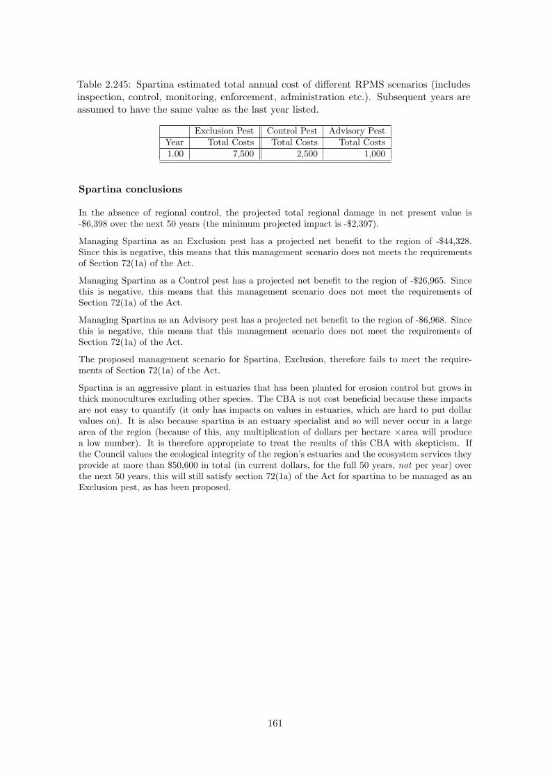
Table 2.245: Spartina estimated total annual cost of di↵erent RPMS scenarios (includesinspection, control, monitoring, enforcement, administration etc.). Subsequent years areassumed to have the same value as the last year listed.
Exclusion Pest Control Pest Advisory PestYear Total Costs Total Costs Total Costs1.00 7,500 2,500 1,000
Spartina conclusions
In the absence of regional control, the projected total regional damage in net present value is-$6,398 over the next 50 years (the minimum projected impact is -$2,397).
Managing Spartina as an Exclusion pest has a projected net benefit to the region of -$44,328.Since this is negative, this means that this management scenario does not meets the requirementsof Section 72(1a) of the Act.
Managing Spartina as a Control pest has a projected net benefit to the region of -$26,965. Sincethis is negative, this means that this management scenario does not meet the requirements ofSection 72(1a) of the Act.
Managing Spartina as an Advisory pest has a projected net benefit to the region of -$6,968. Sincethis is negative, this means that this management scenario does not meet the requirements ofSection 72(1a) of the Act.
The proposed management scenario for Spartina, Exclusion, therefore fails to meet the require-ments of Section 72(1a) of the Act.
Spartina is an aggressive plant in estuaries that has been planted for erosion control but grows inthick monocultures excluding other species. The CBA is not cost beneficial because these impactsare not easy to quantify (it only has impacts on values in estuaries, which are hard to put dollarvalues on). It is also because spartina is an estuary specialist and so will never occur in a largearea of the region (because of this, any multiplication of dollars per hectare ×area will producea low number). It is therefore appropriate to treat the results of this CBA with skepticism. Ifthe Council values the ecological integrity of the region’s estuaries and the ecosystem services theyprovide at more than $50,600 in total (in current dollars, for the full 50 years, not per year) overthe next 50 years, this will still satisfy section 72(1a) of the Act for spartina to be managed as anExclusion pest, as has been proposed.
161

−20 0 20 40 60
0.0
0.2
0.4
0.6
0.8
1.0
Calibrated logistic growth curve, no RPMS control
Years from present
Prop
ortio
n of
max
imum
ext
ent
Current extent (ha): 10
Potential extent (ha): 1,061
(355−−1,766)
Time to potential (yr): 75
Current prop. of potential: 0.017
Figure 2.59: The modelled pest spread until it reaches its anticipated maximum extent.Shown are the results of the average (solid line), minimum (dotted line), and maximum(dashed line) scenarios. (A horizontal line means that the pest has already reached itsmaximum extent.) The vertical dotted-dashed lines indicate the CBA assessment periodused in this report.
162

●●
●●
●●
●●
●●
●●
●●
●●
●●
●●
●●
●●
●●
●●
●●
●●
●●
●●
●●
●●
●●
●●
●●
●●
●●
●
010
2030
4050
050100
150
Popu
latio
n gr
owth
, no
RPM
S co
ntro
l
Year
s fro
m p
rese
nt
Proportion of initial area
●●
●●
●●
●●
●●
●●
●●
●●
●●
●●
●●
●●
●●
●●
●●
●●
●●
●●
●●
●●
●●
●●
●●
●●
●●
●
010
2030
4050
050100
150
Dis
coun
ted
grow
th
Year
s fro
m p
rese
nt
Discounted annual cost
Dis
coun
t rat
e: 0
.08
Tota
l mul
tiplie
r: 13
0.39
(96−−2
58)
(a)
●
●
●
●
●
●
●
●
●
●
02
46
8
0.0
0.2
0.4
0.6
0.8
1.0
Popu
latio
n gr
owth
, exc
lusi
on c
ontro
l
Year
s fro
m p
rese
ntProportion of initial area
●
●
●
●
●
●
●
●
●
●
02
46
8
0.0
0.2
0.4
0.6
0.8
1.0
Dis
coun
ted
grow
th, e
xclu
sion
con
trol
Year
s of
con
trol
Discounted annual cost
(b)
●●
●●
●●
●●
●●
●●
●●
●●
●●
●●
●●
●●
●●
●●
●●
●●
●●
●●
●●
●●
●●
●●
●●
●●
●●
●
010
2030
4050
0.0
0.2
0.4
0.6
0.8
1.0
Popu
latio
n gr
owth
, con
trol c
ontro
l
Year
s fro
m p
rese
nt
Proportion of initial area
●
●
●
●
●
●
●
●
●
●
●
●
●
●
●
●●
●●
●●
●●
●●
●●
●●
●●
●●
●●
●●
●●
●●
●●
●●
●●
●●
●●
010
2030
4050
0.0
0.2
0.4
0.6
0.8
1.0
Dis
coun
ted
grow
th, c
ontro
l con
trol
Year
s of
con
trol
Discounted annual cost
(c)
●
●
●
●
●
●
01
23
45
0.0
0.2
0.4
0.6
0.8
1.0
Popu
latio
n gr
owth
, adv
isor
y co
ntro
l
Year
s fro
m p
rese
nt
Proportion of initial area
●
●
●
●
●
●
01
23
45
0.0
0.2
0.4
0.6
0.8
1.0
Dis
coun
ted
grow
th, a
dvis
ory
cont
rol
Year
s of
con
trol
Discounted annual cost
(d)
Fig
ure
2.60
:T
hem
odel
led
popu
lati
onch
ange
sov
erth
eC
BA
asse
ssm
ent
peri
odfo
r(a
)no
regi
onal
cont
rol,
(b)
Exc
lusi
onPes
tco
ntro
l,(c
)C
ontr
olPes
tco
ntro
l,an
d(d
)A
dvis
ory
Pes
tco
ntro
l.T
heup
per
grap
hssh
owth
epo
pula
tion
chan
ges,
and
the
low
ergr
aphs
show
the
disc
ount
ing
ofas
soci
ated
impa
cts
each
year
(im
pact
sin
the
futu
rear
eof
less
valu
eec
onom
ical
lyth
anim
pact
sof
the
sam
esi
zeno
w).
163

2.1.34 Strawberry dogwood (Dendrobenthamia capitata)
Proposed RPMS Category: Advisory
Overall impact: Moderate
Table 2.246: Relevant biology
Attribute DescriptionForm Bushy evergreen tree to 6 m tall with oval grey-green leaves tapering to
a long point, paler underneath, and densely covered in fine hairs. Paleyellow flowers, red strawberry-like bird-dispersed fruit.
Habitat Disturbed forest, shrubland, grassland.Regional distributionCompetitive abilityReproductive ability Produces viable seed.Dispersal methods Seed dispersed by birds.Resistance to control Unknown.Benefits Fruits are edible and used as a food source by native birds e.g. tui.
Table 2.247: Impact evaluation
Category Currentimpact
Potentialimpact
Comment Source
Species diversity L M-H In USA, other dogwoods grow into densethickets in grasslands which crowd out de-sired grasses, sedges and herbs, and al-ter wildlife habitat. In Australia it shadesand crowds out understorey species in tallopen forest.
1, 2, 3
Threatened species L M 1, 2, 3Soil resources - -Water quality - -Production L L Forms dense stands. 2, 3International trade - -Human health - -Recreation - L Dense stands restrict access. 1, 2Maori culture - L See Recreation. 1, 2Source: 1: Williams & Newfield (2002), 2: Anon. (2009b), 3: Anon. (2007d)
164

Strawberry dogwood CBA results
The following are results for cost-benefit analyses for four scenarios, no regional RPMS control,RPMS control as an Exclusion Pest, RPMS control as a Control Pest, and RPMS control as anAdvisory Pest. For the purposes of the CBA calculations, the pest is assumed to continue expandingwith no regional RPMS control, its spread is assumed to be near-arrested under Advisory Controlbut not reduced, and it is assumed to be successfully reduced to the expected smaller extent whenlisted as a Control Pest, more so as an Exclusion pest.
Table 2.248: Strawberry dogwood CBA results for four RPMS scenarios, presented asnet present value (NPV, $) over 50 years. The expenditure refers to regional expenditureunder the RPMS. Minimum and maximum values are in brackets beneath average values.
Scenario Pest impacts Control benefit Expenditure Net benefitNo RPMS 6,706,675 0 0 -6,706,675
(1,440,478–31,672,939) (-1,440,478 – -31,672,939)
Exclusion Pest 2,537 6,704,138 16,866,597 -10,162,459(646–4,099) (1,439,832–31,668,840) (-15,426,765 – 14,802,243)
Control Pest 6,715 6,699,960 660,608 6,039,352(1,625–11,485) (1,438,853–31,661,454) (778,245 – 31,000,846)
Advisory Pest 3,111 6,703,564 13,212 6,690,352(804–4,939) (1,439,674–31,668,000) (1,426,462 – 31,654,788)
Table 2.249: Strawberry dogwood CBA base assumptions.
Base assumptions ValuesCurrent area infested (ha) 90
Total area potentially infested (ha) 142,263 (47,904–236,623)
Years from naturalisation to total area 25Assessment duration (yr) 50
Weighted average impact per hectare of infested land ($/ha) 6.62 (1.55–11.68)
Any benefits provided by the weed 0Discount rate 0.08
Table 2.250: Strawberry dogwood RPMS Exclusion Pest assumptions.
Exclusion Pest assumptions ValuesYears to achieve objectives 9
Final area infested (ha) 11.2 (0–22.5)
Table 2.251: Strawberry dogwood RPMS Control Pest assumptions.
Control Pest assumptions ValuesYears to achieve objectives 50
Final area infested (ha) 56 (45–68)
Table 2.252: Strawberry dogwood RPMS Advisory Pest assumptions.
Advisory Pest assumptions ValuesYears to achieve objectives 5
165

Final area infested (ha) 112 (90–135)
Table 2.253: Strawberry dogwood estimated total annual cost of di↵erent RPMS scenarios(includes inspection, control, monitoring, enforcement, administration etc.). Subsequentyears are assumed to have the same value as the last year listed.
Exclusion Pest Control Pest Advisory PestYear Total Costs Total Costs Total Costs1.00 2,500,000 50,000 1,000
Strawberry dogwood conclusions
In the absence of regional control, the projected total regional damage in net present value is-$6,706,675 over the next 50 years (the minimum projected impact is -$1,440,478).
Managing Strawberry dogwood as an Exclusion pest has a projected net benefit to the region of-$10,162,459. Since this is negative, this means that this management scenario does not meets therequirements of Section 72(1a) of the Act.
Managing Strawberry dogwood as a Control pest has a projected net benefit to the region of$6,039,352. Since this is positive, this means that this management scenario meets the requirementsof Section 72(1a) of the Act.
Managing Strawberry dogwood as an Advisory pest has a projected net benefit to the region of$6,690,352. Since this is positive, this means that this management scenario meets the requirementsof Section 72(1a) of the Act.
The proposed management scenario for Strawberry dogwood, Advisory, therefore meets the re-quirements of Section 72(1a) of the Act.
166

0 5 10 15 20 25
0.0
0.2
0.4
0.6
0.8
1.0
Calibrated logistic growth curve, no RPMS control
Years from present
Prop
ortio
n of
max
imum
ext
ent
Current extent (ha): 90
Potential extent (ha): 142,263
(47,904−−236,623)
Time to potential (yr): 25
Current prop. of potential: 0.001
Figure 2.61: The modelled pest spread until it reaches its anticipated maximum extent.Shown are the results of the average (solid line), minimum (dotted line), and maximum(dashed line) scenarios. (A horizontal line means that the pest has already reached itsmaximum extent.) The vertical dotted-dashed lines indicate the CBA assessment periodused in this report.
167

●●
●●
●●
●●
●●
●
●
●
●
●
●●
●●
●●
●●
●●
●●
●●
●●
●●
●●
●●
●●
●●
●●
●●
●●
●●
●●
010
2030
4050
0
500
1000
1500
2000
2500
Popu
latio
n gr
owth
, no
RPM
S co
ntro
l
Year
s fro
m p
rese
nt
Proportion of initial area
●●
●●
●●
●●
●●
●●
●●
●●
●●
●●
●●
●●
●●
●●
●●
●●
●●
●●
●●
●●
●●
●●
●●
●●
●●
●
010
2030
4050
0
500
1000
1500
2000
2500
Dis
coun
ted
grow
th
Year
s fro
m p
rese
nt
Discounted annual cost
Dis
coun
t rat
e: 0
.08
Tota
l mul
tiplie
r: 45
15.6
1
(283
0−−1
2711
)
(a)
●
●
●
●
●
●
●
●
●
●
02
46
8
0.0
0.2
0.4
0.6
0.8
1.0
Popu
latio
n gr
owth
, exc
lusi
on c
ontro
l
Year
s fro
m p
rese
ntProportion of initial area
●
●
●
●
●
●
●
●
●
●
02
46
8
0.0
0.2
0.4
0.6
0.8
1.0
Dis
coun
ted
grow
th, e
xclu
sion
con
trol
Year
s of
con
trol
Discounted annual cost
(b)
●●
●●
●●
●●
●●
●●
●●
●●
●●
●●
●●
●●
●●
●●
●●
●●
●●
●●
●●
●●
●●
●●
●●
●●
●●
●
010
2030
4050
0.0
0.2
0.4
0.6
0.8
1.0
Popu
latio
n gr
owth
, con
trol c
ontro
l
Year
s fro
m p
rese
nt
Proportion of initial area
●
●
●
●
●
●
●
●
●
●
●
●
●
●
●
●●
●●
●●
●●
●●
●●
●●
●●
●●
●●
●●
●●
●●
●●
●●
●●
●●
●●
010
2030
4050
0.0
0.2
0.4
0.6
0.8
1.0
Dis
coun
ted
grow
th, c
ontro
l con
trol
Year
s of
con
trol
Discounted annual cost
(c)
●
●
●
●
●
●
01
23
45
0.0
0.2
0.4
0.6
0.8
1.0
Popu
latio
n gr
owth
, adv
isor
y co
ntro
l
Year
s fro
m p
rese
nt
Proportion of initial area
●
●
●
●
●
●
01
23
45
0.0
0.2
0.4
0.6
0.8
1.0
Dis
coun
ted
grow
th, a
dvis
ory
cont
rol
Year
s of
con
trol
Discounted annual cost
(d)
Fig
ure
2.62
:T
hem
odel
led
popu
lati
onch
ange
sov
erth
eC
BA
asse
ssm
ent
peri
odfo
r(a
)no
regi
onal
cont
rol,
(b)
Exc
lusi
onPes
tco
ntro
l,(c
)C
ontr
olPes
tco
ntro
l,an
d(d
)A
dvis
ory
Pes
tco
ntro
l.T
heup
per
grap
hssh
owth
epo
pula
tion
chan
ges,
and
the
low
ergr
aphs
show
the
disc
ount
ing
ofas
soci
ated
impa
cts
each
year
(im
pact
sin
the
futu
rear
eof
less
valu
eec
onom
ical
lyth
anim
pact
sof
the
sam
esi
zeno
w).
168

2.1.35 Variegated thistle (Silybum marianum)
Proposed RPMS Category: Control
Overall impact: Moderate
Table 2.254: Relevant biology
Attribute DescriptionForm Annual or biennial thistle growing up to 2 m high. Leaves are very
prickly. Stem is hollow without spines. Flowers are large (7 cm indiameter) and red/purple in colour, only one flower per stem.
Habitat Roadsides, pastures, gardens, wasteland. Grows best on high fertilitysoils.
Regional distribution Limited distribution in Opotiki region.Competitive ability Very aggressive, forming dense impenetrable stands.Reproductive ability Flowers produce large numbers of seeds which may remain viable for
years.Dispersal methods By wind or inclusion in hay bales.Resistance to control Spread of germination times increases di�culty of control but is suscep-
tible to several herbicides especially in seedling and rosette stage.Benefits Edible (young leaves, peeled young stems, roots, bases of flower heads)
and used as medicinal plant (liver complaints).
Table 2.255: Impact evaluation
Category Currentimpact
Potentialimpact
Comment Source
Species diversity - - 1Threatened species - - 1Soil resources - - 1Water quality - - 1Production L M Forms dense patches, esp. on high fertil-
ity soils. Prickles may damage stock andcan cause nitrate poisoning in cattle andsheep.
2, 3
International trade - - 1Human health - - 1Recreation - M Dense patches of large, spiky plants are
nasty to work through.2, 3
Maori culture - - 1Source: 1: Severinsen (2003), 2: Roy et al. (2004), 3: Environment Bay of Plenty (2005i)
169
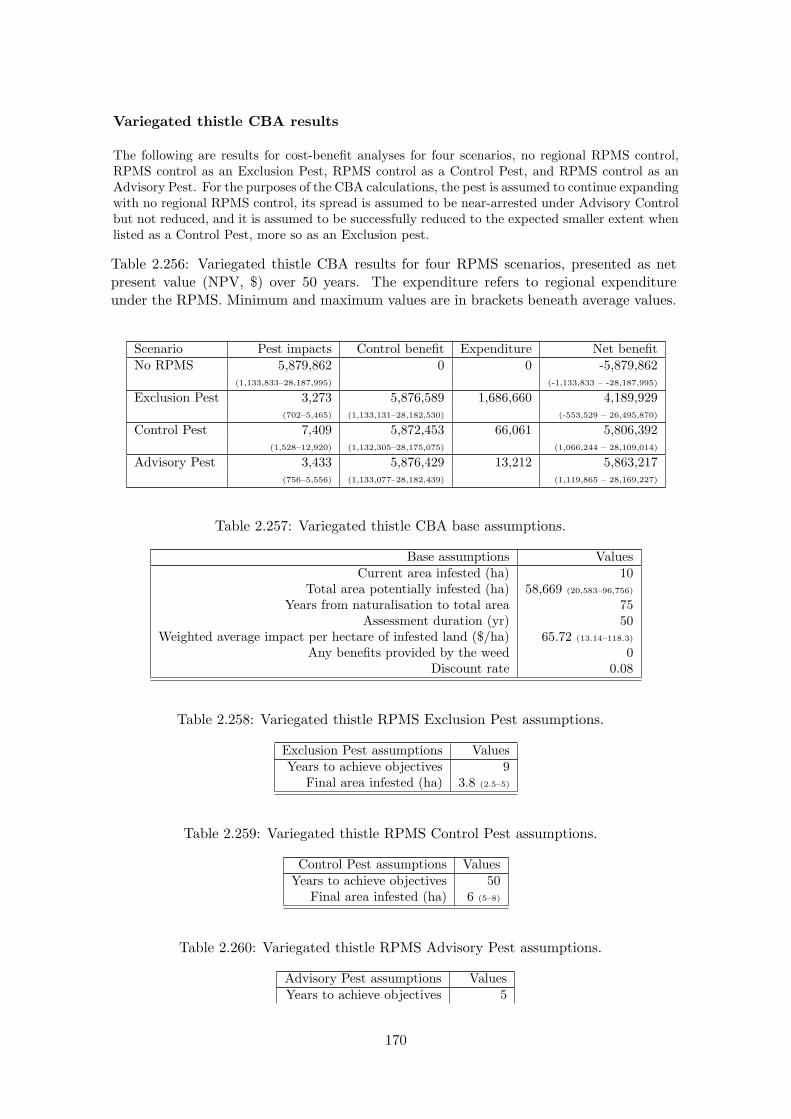
Variegated thistle CBA results
The following are results for cost-benefit analyses for four scenarios, no regional RPMS control,RPMS control as an Exclusion Pest, RPMS control as a Control Pest, and RPMS control as anAdvisory Pest. For the purposes of the CBA calculations, the pest is assumed to continue expandingwith no regional RPMS control, its spread is assumed to be near-arrested under Advisory Controlbut not reduced, and it is assumed to be successfully reduced to the expected smaller extent whenlisted as a Control Pest, more so as an Exclusion pest.
Table 2.256: Variegated thistle CBA results for four RPMS scenarios, presented as netpresent value (NPV, $) over 50 years. The expenditure refers to regional expenditureunder the RPMS. Minimum and maximum values are in brackets beneath average values.
Scenario Pest impacts Control benefit Expenditure Net benefitNo RPMS 5,879,862 0 0 -5,879,862
(1,133,833–28,187,995) (-1,133,833 – -28,187,995)
Exclusion Pest 3,273 5,876,589 1,686,660 4,189,929(702–5,465) (1,133,131–28,182,530) (-553,529 – 26,495,870)
Control Pest 7,409 5,872,453 66,061 5,806,392(1,528–12,920) (1,132,305–28,175,075) (1,066,244 – 28,109,014)
Advisory Pest 3,433 5,876,429 13,212 5,863,217(756–5,556) (1,133,077–28,182,439) (1,119,865 – 28,169,227)
Table 2.257: Variegated thistle CBA base assumptions.
Base assumptions ValuesCurrent area infested (ha) 10
Total area potentially infested (ha) 58,669 (20,583–96,756)
Years from naturalisation to total area 75Assessment duration (yr) 50
Weighted average impact per hectare of infested land ($/ha) 65.72 (13.14–118.3)
Any benefits provided by the weed 0Discount rate 0.08
Table 2.258: Variegated thistle RPMS Exclusion Pest assumptions.
Exclusion Pest assumptions ValuesYears to achieve objectives 9
Final area infested (ha) 3.8 (2.5–5)
Table 2.259: Variegated thistle RPMS Control Pest assumptions.
Control Pest assumptions ValuesYears to achieve objectives 50
Final area infested (ha) 6 (5–8)
Table 2.260: Variegated thistle RPMS Advisory Pest assumptions.
Advisory Pest assumptions ValuesYears to achieve objectives 5
170
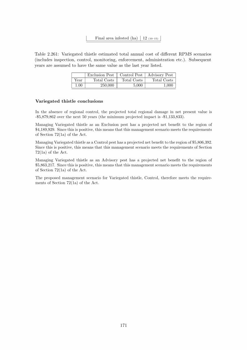
Final area infested (ha) 12 (10–15)
Table 2.261: Variegated thistle estimated total annual cost of di↵erent RPMS scenarios(includes inspection, control, monitoring, enforcement, administration etc.). Subsequentyears are assumed to have the same value as the last year listed.
Exclusion Pest Control Pest Advisory PestYear Total Costs Total Costs Total Costs1.00 250,000 5,000 1,000
Variegated thistle conclusions
In the absence of regional control, the projected total regional damage in net present value is-$5,879,862 over the next 50 years (the minimum projected impact is -$1,133,833).
Managing Variegated thistle as an Exclusion pest has a projected net benefit to the region of$4,189,929. Since this is positive, this means that this management scenario meets the requirementsof Section 72(1a) of the Act.
Managing Variegated thistle as a Control pest has a projected net benefit to the region of $5,806,392.Since this is positive, this means that this management scenario meets the requirements of Section72(1a) of the Act.
Managing Variegated thistle as an Advisory pest has a projected net benefit to the region of$5,863,217. Since this is positive, this means that this management scenario meets the requirementsof Section 72(1a) of the Act.
The proposed management scenario for Variegated thistle, Control, therefore meets the require-ments of Section 72(1a) of the Act.
171

0 20 40 60
0.0
0.2
0.4
0.6
0.8
1.0
Calibrated logistic growth curve, no RPMS control
Years from present
Prop
ortio
n of
max
imum
ext
ent
Current extent (ha): 10
Potential extent (ha): 58,669
(20,583−−96,756)
Time to potential (yr): 75
Current prop. of potential: <0.01
Figure 2.63: The modelled pest spread until it reaches its anticipated maximum extent.Shown are the results of the average (solid line), minimum (dotted line), and maximum(dashed line) scenarios. (A horizontal line means that the pest has already reached itsmaximum extent.) The vertical dotted-dashed lines indicate the CBA assessment periodused in this report.
172

●●
●●
●●
●●
●●
●●
●●
●●
●●
●●
●●
●●
●●
●●
●●
●●
●●
●●
●●
●●
●●
●●
●●
●●
●●
●
010
2030
4050
0
2000
4000
6000
8000
Popu
latio
n gr
owth
, no
RPM
S co
ntro
l
Year
s fro
m p
rese
nt
Proportion of initial area
●●
●●
●●
●●
●●
●●
●●
●●
●●
●●
●●
●●
●●
●●
●●
●●
●●
●●
●●
●●
●●
●●
●●
●●
●●
●
010
2030
4050
0
2000
4000
6000
8000
Dis
coun
ted
grow
th
Year
s fro
m p
rese
nt
Discounted annual cost
Dis
coun
t rat
e: 0
.08
Tota
l mul
tiplie
r: 22
79.1
2
(138
2−−6
495)
(a)
●
●
●
●
●
●
●
●
●
●
02
46
8
0.0
0.2
0.4
0.6
0.8
1.0
Popu
latio
n gr
owth
, exc
lusi
on c
ontro
l
Year
s fro
m p
rese
ntProportion of initial area
●
●
●
●
●
●
●
●
●
●
02
46
8
0.0
0.2
0.4
0.6
0.8
1.0
Dis
coun
ted
grow
th, e
xclu
sion
con
trol
Year
s of
con
trol
Discounted annual cost
(b)
●●
●●
●●
●●
●●
●●
●●
●●
●●
●●
●●
●●
●●
●●
●●
●●
●●
●●
●●
●●
●●
●●
●●
●●
●●
●
010
2030
4050
0.0
0.2
0.4
0.6
0.8
1.0
Popu
latio
n gr
owth
, con
trol c
ontro
l
Year
s fro
m p
rese
nt
Proportion of initial area
●
●
●
●
●
●
●
●
●
●
●
●
●
●
●
●●
●●
●●
●●
●●
●●
●●
●●
●●
●●
●●
●●
●●
●●
●●
●●
●●
●●
010
2030
4050
0.0
0.2
0.4
0.6
0.8
1.0
Dis
coun
ted
grow
th, c
ontro
l con
trol
Year
s of
con
trol
Discounted annual cost
(c)
●
●
●
●
●
●
01
23
45
0.0
0.2
0.4
0.6
0.8
1.0
Popu
latio
n gr
owth
, adv
isor
y co
ntro
l
Year
s fro
m p
rese
nt
Proportion of initial area
●
●
●
●
●
●
01
23
45
0.0
0.2
0.4
0.6
0.8
1.0
Dis
coun
ted
grow
th, a
dvis
ory
cont
rol
Year
s of
con
trol
Discounted annual cost
(d)
Fig
ure
2.64
:T
hem
odel
led
popu
lati
onch
ange
sov
erth
eC
BA
asse
ssm
ent
peri
odfo
r(a
)no
regi
onal
cont
rol,
(b)
Exc
lusi
onPes
tco
ntro
l,(c
)C
ontr
olPes
tco
ntro
l,an
d(d
)A
dvis
ory
Pes
tco
ntro
l.T
heup
per
grap
hssh
owth
epo
pula
tion
chan
ges,
and
the
low
ergr
aphs
show
the
disc
ount
ing
ofas
soci
ated
impa
cts
each
year
(im
pact
sin
the
futu
rear
eof
less
valu
eec
onom
ical
lyth
anim
pact
sof
the
sam
esi
zeno
w).
173
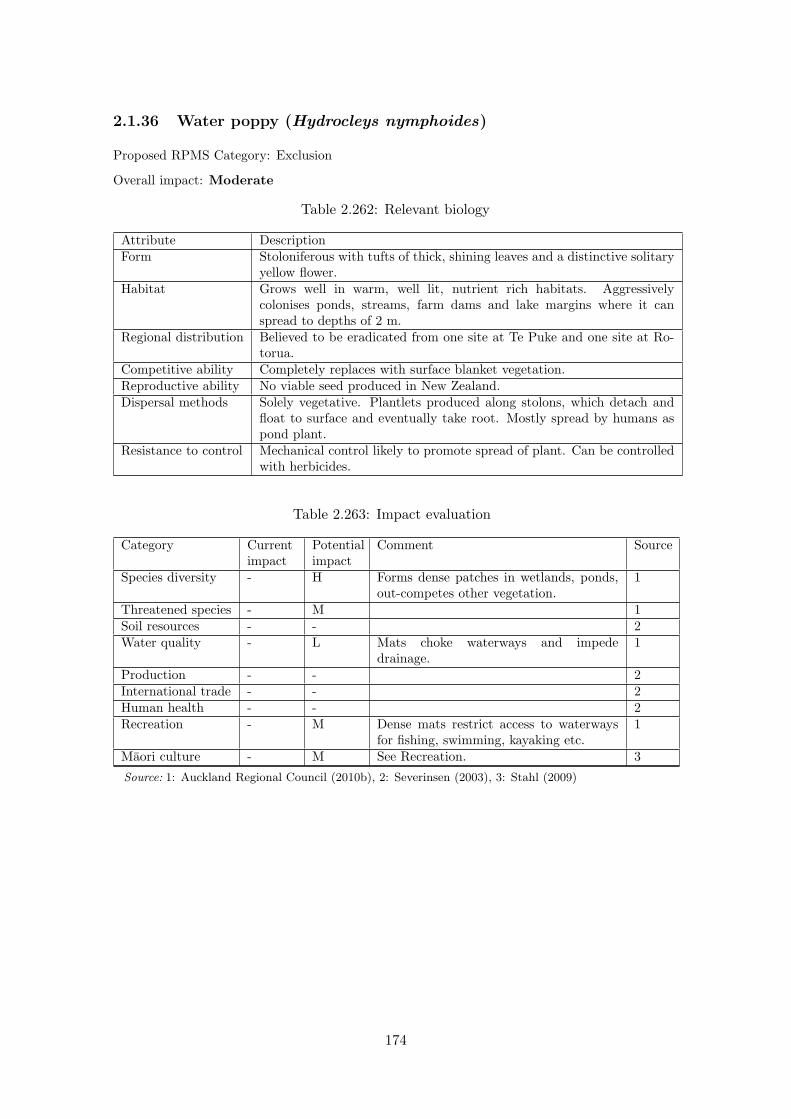
2.1.36 Water poppy (Hydrocleys nymphoides)
Proposed RPMS Category: Exclusion
Overall impact: Moderate
Table 2.262: Relevant biology
Attribute DescriptionForm Stoloniferous with tufts of thick, shining leaves and a distinctive solitary
yellow flower.Habitat Grows well in warm, well lit, nutrient rich habitats. Aggressively
colonises ponds, streams, farm dams and lake margins where it canspread to depths of 2 m.
Regional distribution Believed to be eradicated from one site at Te Puke and one site at Ro-torua.
Competitive ability Completely replaces with surface blanket vegetation.Reproductive ability No viable seed produced in New Zealand.Dispersal methods Solely vegetative. Plantlets produced along stolons, which detach and
float to surface and eventually take root. Mostly spread by humans aspond plant.
Resistance to control Mechanical control likely to promote spread of plant. Can be controlledwith herbicides.
Table 2.263: Impact evaluation
Category Currentimpact
Potentialimpact
Comment Source
Species diversity - H Forms dense patches in wetlands, ponds,out-competes other vegetation.
1
Threatened species - M 1Soil resources - - 2Water quality - L Mats choke waterways and impede
drainage.1
Production - - 2International trade - - 2Human health - - 2Recreation - M Dense mats restrict access to waterways
for fishing, swimming, kayaking etc.1
Maori culture - M See Recreation. 3Source: 1: Auckland Regional Council (2010b), 2: Severinsen (2003), 3: Stahl (2009)
174

Water poppy CBA results
Since Water poppy is currently absent from the region, it is di�cult to accurately quantify thecosts and benefits of current and proposed e↵orts to continue to exclude the species. If the specieswere to invade this year and spread in the region, without regional control for the next 50 years,the total pest impacts over this period in net present value are calculated to be $106,639 ($47,878–$188,615). This can be compared with the calculated net present value of the proposed annualexpenditure on control over this same period of $6,747 (Exclusion pest). Note that this comparisondoes not take into account whether or not the proposed level of expenditure is adequate to havea high probability of excluding the species over this period. Given the broad experience of thebiosecurity sta↵ at Environment Bay of Plenty, we assume that it will be.
The following tables provide the parameters used in this cost-benefit analysis.
Table 2.264: Water poppy CBA base assumptions.
Base assumptions ValuesCurrent area infested (ha) 0
Total area potentially infested (ha) 4,216 (1,405–7,027)
Years from naturalisation to total area 100Assessment duration (yr) 50
Weighted average impact per hectare of infested land ($/ha) 1 (1–1)
Any benefits provided by the weed 0Discount rate 0.08
Table 2.265: Water poppy estimated total annual cost of the proposed RPMS scenario(includes inspection, control, monitoring, enforcement, administration etc.). Subsequentyears are assumed to have the same value as the last year listed.
Exclusion PestYear Total Costs1.00 1,000
Water poppy conclusions
Since the calculated average impact should the species invade is greater than the anticipated expen-diture, and regional establishment is likely in the absence of regional surveillance and preparationsfor rapid response, this management scenario meets the requirements of Section 72(1a) of theAct.
175
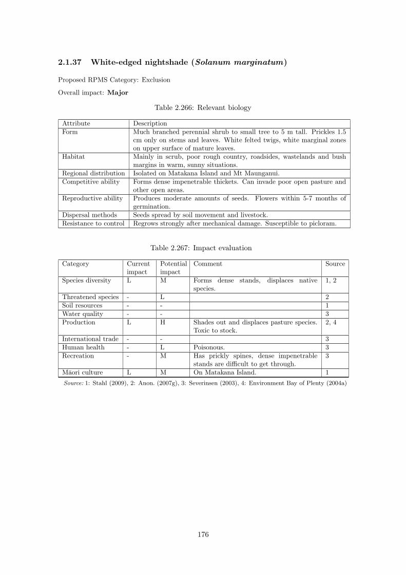
2.1.37 White-edged nightshade (Solanum marginatum)
Proposed RPMS Category: Exclusion
Overall impact: Major
Table 2.266: Relevant biology
Attribute DescriptionForm Much branched perennial shrub to small tree to 5 m tall. Prickles 1.5
cm only on stems and leaves. White felted twigs, white marginal zoneson upper surface of mature leaves.
Habitat Mainly in scrub, poor rough country, roadsides, wastelands and bushmargins in warm, sunny situations.
Regional distribution Isolated on Matakana Island and Mt Maunganui.Competitive ability Forms dense impenetrable thickets. Can invade poor open pasture and
other open areas.Reproductive ability Produces moderate amounts of seeds. Flowers within 5-7 months of
germination.Dispersal methods Seeds spread by soil movement and livestock.Resistance to control Regrows strongly after mechanical damage. Susceptible to picloram.
Table 2.267: Impact evaluation
Category Currentimpact
Potentialimpact
Comment Source
Species diversity L M Forms dense stands, displaces nativespecies.
1, 2
Threatened species - L 2Soil resources - - 1Water quality - - 3Production L H Shades out and displaces pasture species.
Toxic to stock.2, 4
International trade - - 3Human health - L Poisonous. 3Recreation - M Has prickly spines, dense impenetrable
stands are di�cult to get through.3
Maori culture L M On Matakana Island. 1Source: 1: Stahl (2009), 2: Anon. (2007g), 3: Severinsen (2003), 4: Environment Bay of Plenty (2004a)
176

White-edged nightshade CBA results
The following are results for cost-benefit analyses for four scenarios, no regional RPMS control,RPMS control as an Exclusion Pest, RPMS control as a Control Pest, and RPMS control as anAdvisory Pest. For the purposes of the CBA calculations, the pest is assumed to continue expandingwith no regional RPMS control, its spread is assumed to be near-arrested under Advisory Controlbut not reduced, and it is assumed to be successfully reduced to the expected smaller extent whenlisted as a Control Pest, more so as an Exclusion pest.
Table 2.268: White-edged nightshade CBA results for four RPMS scenarios, presented asnet present value (NPV, $) over 50 years. The expenditure refers to regional expenditureunder the RPMS. Minimum and maximum values are in brackets beneath average values.
Scenario Pest impacts Control benefit Expenditure Net benefitNo RPMS 37,143,299 0 0 -37,143,299
(14,675,917–149,407,198) (-14,675,917 – -149,407,198)
Exclusion Pest 2,151 37,141,148 10,120 37,131,028(457–3,627) (14,675,460–149,403,571) (14,665,340 – 149,393,451)
Control Pest 4,518 37,138,781 13,212 37,125,569(920–7,990) (14,674,997–149,399,208) (14,661,785 – 149,385,996)
Advisory Pest 1,990 37,141,309 6,606 37,134,703(362–3,904) (14,675,555–149,403,294) (14,668,949 – 149,396,688)
Table 2.269: White-edged nightshade CBA base assumptions.
Base assumptions ValuesCurrent area infested (ha) 6
Total area potentially infested (ha) 130,154 (43,408–216,901)
Years from naturalisation to total area 50Assessment duration (yr) 50
Weighted average impact per hectare of infested land ($/ha) 62.88 (12.58–113.18)
Any benefits provided by the weed 0Discount rate 0.08
Table 2.270: White-edged nightshade RPMS Exclusion Pest assumptions.
Exclusion Pest assumptions ValuesYears to achieve objectives 9
Final area infested (ha) 3.8 (3–4.5)
Table 2.271: White-edged nightshade RPMS Control Pest assumptions.
Control Pest assumptions ValuesYears to achieve objectives 50
Final area infested (ha) 5 (5–6)
Table 2.272: White-edged nightshade RPMS Advisory Pest assumptions.
Advisory Pest assumptions ValuesYears to achieve objectives 5
177

Final area infested (ha) 8 (9–6)
Table 2.273: White-edged nightshade estimated total annual cost of di↵erent RPMS sce-narios (includes inspection, control, monitoring, enforcement, administration etc.). Sub-sequent years are assumed to have the same value as the last year listed.
Exclusion Pest Control Pest Advisory PestYear Total Costs Total Costs Total Costs1.00 1,500 1,000 500
White-edged nightshade conclusions
In the absence of regional control, the projected total regional damage in net present value is-$37,143,299 over the next 50 years (the minimum projected impact is -$14,675,917).
Managing White-edged nightshade as an Exclusion pest has a projected net benefit to the re-gion of $37,131,028. Since this is positive, this means that this management scenario meets therequirements of Section 72(1a) of the Act.
Managing White-edged nightshade as a Control pest has a projected net benefit to the region of$37,125,569. Since this is positive, this means that this management scenario meets the require-ments of Section 72(1a) of the Act.
Managing White-edged nightshade as an Advisory pest has a projected net benefit to the re-gion of $37,134,703. Since this is positive, this means that this management scenario meets therequirements of Section 72(1a) of the Act.
The proposed management scenario for White-edged nightshade, Exclusion, therefore meets therequirements of Section 72(1a) of the Act.
178

0 10 20 30 40 50
0.0
0.2
0.4
0.6
0.8
1.0
Calibrated logistic growth curve, no RPMS control
Years from present
Prop
ortio
n of
max
imum
ext
ent
Current extent (ha): 6
Potential extent (ha): 130,154
(43,408−−216,901)
Time to potential (yr): 50
Current prop. of potential: <0.01
Figure 2.65: The modelled pest spread until it reaches its anticipated maximum extent.Shown are the results of the average (solid line), minimum (dotted line), and maximum(dashed line) scenarios. (A horizontal line means that the pest has already reached itsmaximum extent.) The vertical dotted-dashed lines indicate the CBA assessment periodused in this report.
179
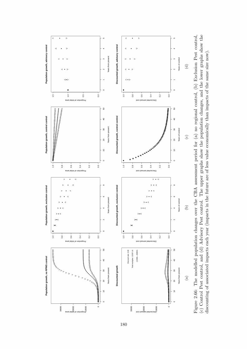
●●
●●
●●
●●
●●
●●
●●
●●
●●
●●
●●
●
●
●
●
●
●
●●
●●
●●
●●
●●
●●
●●
●●
●●
●●
●●
●
010
2030
4050
0
1000
0
2000
0
3000
0
Popu
latio
n gr
owth
, no
RPM
S co
ntro
l
Year
s fro
m p
rese
nt
Proportion of initial area
●●
●●
●●
●●
●●
●●
●●
●●
●●
●●
●●
●●
●●
●●
●●
●●
●●
●●
●●
●●
●●
●●
●●
●●
●●
●
010
2030
4050
0
1000
0
2000
0
3000
0
Dis
coun
ted
grow
th
Year
s fro
m p
rese
nt
Discounted annual cost
Dis
coun
t rat
e: 0
.08
Tota
l mul
tiplie
r: 22
307.
16
(133
86−−
6688
4)
(a)
●
●
●
●
●
●
●
●
●
●
02
46
8
0.0
0.2
0.4
0.6
0.8
1.0
Popu
latio
n gr
owth
, exc
lusi
on c
ontro
l
Year
s fro
m p
rese
ntProportion of initial area
●
●
●
●
●
●
●
●
●
●
02
46
8
0.0
0.2
0.4
0.6
0.8
1.0
Dis
coun
ted
grow
th, e
xclu
sion
con
trol
Year
s of
con
trol
Discounted annual cost
(b)
●●
●●
●●
●●
●●
●●
●●
●●
●●
●●
●●
●●
●●
●●
●●
●●
●●
●●
●●
●●
●●
●●
●●
●●
●●
●
010
2030
4050
0.0
0.2
0.4
0.6
0.8
1.0
Popu
latio
n gr
owth
, con
trol c
ontro
l
Year
s fro
m p
rese
nt
Proportion of initial area
●
●
●
●
●
●
●
●
●
●
●
●
●
●
●
●●
●●
●●
●●
●●
●●
●●
●●
●●
●●
●●
●●
●●
●●
●●
●●
●●
●●
010
2030
4050
0.0
0.2
0.4
0.6
0.8
1.0
Dis
coun
ted
grow
th, c
ontro
l con
trol
Year
s of
con
trol
Discounted annual cost
(c)
●
●
●
●
●
●
01
23
45
0.0
0.5
1.0
1.5
Popu
latio
n gr
owth
, adv
isor
y co
ntro
l
Year
s fro
m p
rese
nt
Proportion of initial area
●
●
●
●
●
●
01
23
45
0.0
0.2
0.4
0.6
0.8
1.0
Dis
coun
ted
grow
th, a
dvis
ory
cont
rol
Year
s of
con
trol
Discounted annual cost
(d)
Fig
ure
2.66
:T
hem
odel
led
popu
lati
onch
ange
sov
erth
eC
BA
asse
ssm
ent
peri
odfo
r(a
)no
regi
onal
cont
rol,
(b)
Exc
lusi
onPes
tco
ntro
l,(c
)C
ontr
olPes
tco
ntro
l,an
d(d
)A
dvis
ory
Pes
tco
ntro
l.T
heup
per
grap
hssh
owth
epo
pula
tion
chan
ges,
and
the
low
ergr
aphs
show
the
disc
ount
ing
ofas
soci
ated
impa
cts
each
year
(im
pact
sin
the
futu
rear
eof
less
valu
eec
onom
ical
lyth
anim
pact
sof
the
sam
esi
zeno
w).
180

2.1.38 Wild ginger (yellow and kahili) (Hedychium gardnerianum, H.flavescens)
Proposed RPMS Category: Control
Overall impact: Major
Table 2.274: Relevant biology
Attribute DescriptionForm Both gingers have large green leaves with spikes and scented flowers and
can grow up to 2-3 m tall, with massive branching surface rhizomes.Flowers of kahili ginger are yellow with red stamens. Yellow ginger hascreamy flowers.
Habitat Thrives in warm damp areas, very shade tolerant.Regional distribution Found in most parts of region.Competitive ability Both gingers spread rapidly from large rhizomes which form thick mats
up to 1 m deep in the soil. Can suppress 90% of native vegetation.Reproductive ability Kahili ginger produces up to 100 seeds per head. Yellow ginger does not
produce seed.Dispersal methods Kahili ginger produces seed which is spread by birds. Spread also by
dumping garden waste.Resistance to control Can be controlled using herbicides. Removal by hand di�cult due to
size of rhizomes.
Table 2.275: Impact evaluation
Category Currentimpact
Potentialimpact
Comment Source
Species diversity M H Forms dense patches and out-competes al-most all native species, prevents forest re-generation.
1, 2
Threatened species L H 1, 2Soil resources - L Shallow-rooted, deep rhizome beds be-
come heavy with rain and slip on steepsites and streambanks, causing erosion.
1
Water quality - - 3Production L L Established in pine blocks. 4, 5International trade - - 3Human health - - 3Recreation L M Dense patches restrict access. 3Maori culture L M Obstructs access to cultural sites (e.g.
waahi tapu, urupa).3
Source: 1: Craw (2000), 2: Williams et al. (2003), 3: Severinsen (2003), 4: Department of Conservation(1997b), 5: Mather (2009)
181

Wild ginger (yellow and kahili) CBA results
The following are results for cost-benefit analyses for four scenarios, no regional RPMS control,RPMS control as an Exclusion Pest, RPMS control as a Control Pest, and RPMS control as anAdvisory Pest. For the purposes of the CBA calculations, the pest is assumed to continue expandingwith no regional RPMS control, its spread is assumed to be near-arrested under Advisory Controlbut not reduced, and it is assumed to be successfully reduced to the expected smaller extent whenlisted as a Control Pest, more so as an Exclusion pest.
Table 2.276: Wild ginger (yellow and kahili) CBA results for four RPMS scenarios, pre-sented as net present value (NPV, $) over 50 years. The expenditure refers to regionalexpenditure under the RPMS. Minimum and maximum values are in brackets beneathaverage values.
Scenario Pest impacts Control benefit Expenditure Net benefitNo RPMS 1,388,662 0 0 -1,388,662
(331,515–4,181,345) (-331,515 – -4,181,345)
Exclusion Pest 44,659 1,344,003 15,854,602 -14,510,599(10,622–72,788) (320,893–4,108,557) (-15,533,709 – -11,746,045)
Control Pest 118,216 1,270,446 620,972 649,474(26,730–203,947) (304,785–3,977,398) (-316,187 – 3,356,426)
Advisory Pest 54,773 1,333,889 13,212 1,320,677(13,220–87,710) (318,295–4,093,635) (305,083 – 4,080,423)
Table 2.277: Wild ginger (yellow and kahili) CBA base assumptions.
Base assumptions ValuesCurrent area infested (ha) 700
Total area potentially infested (ha) 100,702 (34,134–167,271)
Years from naturalisation to total area 75Assessment duration (yr) 50
Weighted average impact per hectare of infested land ($/ha) 14.98 (3.28–26.68)
Any benefits provided by the weed 0Discount rate 0.08
Table 2.278: Wild ginger (yellow and kahili) RPMS Exclusion Pest assumptions.
Exclusion Pest assumptions ValuesYears to achieve objectives 9
Final area infested (ha) 87.5 (0–175)
Table 2.279: Wild ginger (yellow and kahili) RPMS Control Pest assumptions.
Control Pest assumptions ValuesYears to achieve objectives 50
Final area infested (ha) 438 (350–525)
Table 2.280: Wild ginger (yellow and kahili) RPMS Advisory Pest assumptions.
Advisory Pest assumptions ValuesYears to achieve objectives 5
182
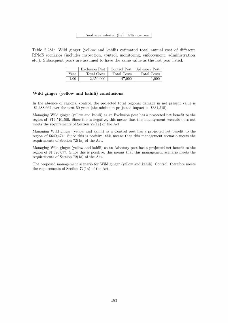
Final area infested (ha) 875 (700–1,050)
Table 2.281: Wild ginger (yellow and kahili) estimated total annual cost of di↵erentRPMS scenarios (includes inspection, control, monitoring, enforcement, administrationetc.). Subsequent years are assumed to have the same value as the last year listed.
Exclusion Pest Control Pest Advisory PestYear Total Costs Total Costs Total Costs1.00 2,350,000 47,000 1,000
Wild ginger (yellow and kahili) conclusions
In the absence of regional control, the projected total regional damage in net present value is-$1,388,662 over the next 50 years (the minimum projected impact is -$331,515).
Managing Wild ginger (yellow and kahili) as an Exclusion pest has a projected net benefit to theregion of -$14,510,599. Since this is negative, this means that this management scenario does notmeets the requirements of Section 72(1a) of the Act.
Managing Wild ginger (yellow and kahili) as a Control pest has a projected net benefit to theregion of $649,474. Since this is positive, this means that this management scenario meets therequirements of Section 72(1a) of the Act.
Managing Wild ginger (yellow and kahili) as an Advisory pest has a projected net benefit to theregion of $1,320,677. Since this is positive, this means that this management scenario meets therequirements of Section 72(1a) of the Act.
The proposed management scenario for Wild ginger (yellow and kahili), Control, therefore meetsthe requirements of Section 72(1a) of the Act.
183

−20 0 20 40 60
0.0
0.2
0.4
0.6
0.8
1.0
Calibrated logistic growth curve, no RPMS control
Years from present
Prop
ortio
n of
max
imum
ext
ent
Current extent (ha): 700
Potential extent (ha): 100,702
(34,134−−167,271)
Time to potential (yr): 75
Current prop. of potential: 0.012
Figure 2.67: The modelled pest spread until it reaches its anticipated maximum extent.Shown are the results of the average (solid line), minimum (dotted line), and maximum(dashed line) scenarios. (A horizontal line means that the pest has already reached itsmaximum extent.) The vertical dotted-dashed lines indicate the CBA assessment periodused in this report.
184

●●
●●
●●
●●
●●
●●
●●
●●
●●
●●
●●
●●
●●
●●
●●
●●
●●
●●
●●
●●
●●
●●
●●
●●
●●
●
010
2030
4050
050100
150
200
Popu
latio
n gr
owth
, no
RPM
S co
ntro
l
Year
s fro
m p
rese
nt
Proportion of initial area
●●
●●
●●
●●
●●
●●
●●
●●
●●
●●
●●
●●
●●
●●
●●
●●
●●
●●
●●
●●
●●
●●
●●
●●
●●
●
010
2030
4050
050100
150
200
Dis
coun
ted
grow
th
Year
s fro
m p
rese
nt
Discounted annual cost
Dis
coun
t rat
e: 0
.08
Tota
l mul
tiplie
r: 15
8.03
(116−−
313)
(a)
●
●
●
●
●
●
●
●
●
●
02
46
8
0.0
0.2
0.4
0.6
0.8
1.0
Popu
latio
n gr
owth
, exc
lusi
on c
ontro
l
Year
s fro
m p
rese
ntProportion of initial area
●
●
●
●
●
●
●
●
●
●
02
46
8
0.0
0.2
0.4
0.6
0.8
1.0
Dis
coun
ted
grow
th, e
xclu
sion
con
trol
Year
s of
con
trol
Discounted annual cost
(b)
●●
●●
●●
●●
●●
●●
●●
●●
●●
●●
●●
●●
●●
●●
●●
●●
●●
●●
●●
●●
●●
●●
●●
●●
●●
●
010
2030
4050
0.0
0.2
0.4
0.6
0.8
1.0
Popu
latio
n gr
owth
, con
trol c
ontro
l
Year
s fro
m p
rese
nt
Proportion of initial area
●
●
●
●
●
●
●
●
●
●
●
●
●
●
●
●●
●●
●●
●●
●●
●●
●●
●●
●●
●●
●●
●●
●●
●●
●●
●●
●●
●●
010
2030
4050
0.0
0.2
0.4
0.6
0.8
1.0
Dis
coun
ted
grow
th, c
ontro
l con
trol
Year
s of
con
trol
Discounted annual cost
(c)
●
●
●
●
●
●
01
23
45
0.0
0.2
0.4
0.6
0.8
1.0
Popu
latio
n gr
owth
, adv
isor
y co
ntro
l
Year
s fro
m p
rese
nt
Proportion of initial area
●
●
●
●
●
●
01
23
45
0.0
0.2
0.4
0.6
0.8
1.0
Dis
coun
ted
grow
th, a
dvis
ory
cont
rol
Year
s of
con
trol
Discounted annual cost
(d)
Fig
ure
2.68
:T
hem
odel
led
popu
lati
onch
ange
sov
erth
eC
BA
asse
ssm
ent
peri
odfo
r(a
)no
regi
onal
cont
rol,
(b)
Exc
lusi
onPes
tco
ntro
l,(c
)C
ontr
olPes
tco
ntro
l,an
d(d
)A
dvis
ory
Pes
tco
ntro
l.T
heup
per
grap
hssh
owth
epo
pula
tion
chan
ges,
and
the
low
ergr
aphs
show
the
disc
ount
ing
ofas
soci
ated
impa
cts
each
year
(im
pact
sin
the
futu
rear
eof
less
valu
eec
onom
ical
lyth
anim
pact
sof
the
sam
esi
zeno
w).
185

2.1.39 Wild kiwifruit (Actinidia spp.)
Proposed RPMS Category: Control
Overall impact: Major
Table 2.282: Relevant biology
Attribute DescriptionForm Vigorous perennial vine up to 15 m. Climbing or straggling.Habitat Exotic and native forest, particularly on the margins and in light gaps,
regenerating forest, riparian margins, and scrub. Usually close to ki-wifruit orchards or where excess fruit has been dumped or fed to stock.
Regional distribution Te Puke and Katikati areas, isolated elsewhere.Competitive ability Can smother or strangle host plants. Very vigorous grower.Reproductive ability Each fruit contains numerous small seeds.Dispersal methods Birds and stock can spread seed. Fruit also distributed by dumping or
used as stock food for cattle and deer.Resistance to control Can be cut and treated with herbicide or sprayed during spring and
summer.Benefits Edible fruit. Reject export fruit used as livestock feed.
Table 2.283: Impact evaluation
Category Currentimpact
Potentialimpact
Comment Source
Species diversity L H Smothers canopy trees with dense vinesand causes collapse.
1
Threatened species - M 1Soil resources - - 2Water quality - - 2Production L M Smothers trees in plantation forests and
orchards. Prevents access and createssafety hazard during harvest of plantationtrees.
3, 4
International trade - - 2Human health - - 2Recreation - M Dense walls of vines restrict access to for-
est.2
Maori culture - L See Recreation. 2Source: 1: Gianotti (2002), 2: Severinsen (2003), 3: Environment Bay of Plenty (2004a), 4: Environment
Bay of Plenty (2005e)
186

Wild kiwifruit CBA results
The following are results for cost-benefit analyses for four scenarios, no regional RPMS control,RPMS control as an Exclusion Pest, RPMS control as a Control Pest, and RPMS control as anAdvisory Pest. For the purposes of the CBA calculations, the pest is assumed to continue expandingwith no regional RPMS control, its spread is assumed to be near-arrested under Advisory Controlbut not reduced, and it is assumed to be successfully reduced to the expected smaller extent whenlisted as a Control Pest, more so as an Exclusion pest.
Table 2.284: Wild kiwifruit CBA results for four RPMS scenarios, presented as net presentvalue (NPV, $) over 50 years. The expenditure refers to regional expenditure under theRPMS. Minimum and maximum values are in brackets beneath average values.
Scenario Pest impacts Control benefit Expenditure Net benefitNo RPMS 1,417,966 0 0 -1,417,966
(364,748–6,652,469) (-364,748 – -6,652,469)
Exclusion Pest 2,940 1,415,026 10,119,958 -8,704,932(638–4,845) (364,110–6,647,624) (-9,755,848 – -3,472,334)
Control Pest 7,783 1,410,183 396,365 1,013,818(1,604–13,574) (363,144–6,638,895) (-33,221 – 6,242,530)
Advisory Pest 3,606 1,414,360 13,212 1,401,148(793–5,838) (363,955–6,646,631) (350,743 – 6,633,419)
Table 2.285: Wild kiwifruit CBA base assumptions.
Base assumptions ValuesCurrent area infested (ha) 50
Total area potentially infested (ha) 143,637 (48,341–238,933)
Years from naturalisation to total area 100Assessment duration (yr) 50
Weighted average impact per hectare of infested land ($/ha) 13.81 (2.76–24.86)
Any benefits provided by the weed 0Discount rate 0.08
Table 2.286: Wild kiwifruit RPMS Exclusion Pest assumptions.
Exclusion Pest assumptions ValuesYears to achieve objectives 9
Final area infested (ha) 6.2 (0–12.5)
Table 2.287: Wild kiwifruit RPMS Control Pest assumptions.
Control Pest assumptions ValuesYears to achieve objectives 50
Final area infested (ha) 31 (25–38)
Table 2.288: Wild kiwifruit RPMS Advisory Pest assumptions.
Advisory Pest assumptions ValuesYears to achieve objectives 5
Final area infested (ha) 62 (50–75)
187

Table 2.289: Wild kiwifruit estimated total annual cost of di↵erent RPMS scenarios (in-cludes inspection, control, monitoring, enforcement, administration etc.). Subsequentyears are assumed to have the same value as the last year listed.
Exclusion Pest Control Pest Advisory PestYear Total Costs Total Costs Total Costs1.00 1,500,000 30,000 1,000
Wild kiwifruit conclusions
In the absence of regional control, the projected total regional damage in net present value is-$1,417,966 over the next 50 years (the minimum projected impact is -$364,748).
Managing Wild kiwifruit as an Exclusion pest has a projected net benefit to the region of -$8,704,932. Since this is negative, this means that this management scenario does not meetsthe requirements of Section 72(1a) of the Act.
Managing Wild kiwifruit as a Control pest has a projected net benefit to the region of $1,013,818.Since this is positive, this means that this management scenario meets the requirements of Section72(1a) of the Act.
Managing Wild kiwifruit as an Advisory pest has a projected net benefit to the region of $1,401,148.Since this is positive, this means that this management scenario meets the requirements of Section72(1a) of the Act.
The proposed management scenario for Wild kiwifruit, Control, therefore meets the requirementsof Section 72(1a) of the Act.
188

0 20 40 60 80 100
0.0
0.2
0.4
0.6
0.8
1.0
Calibrated logistic growth curve, no RPMS control
Years from present
Prop
ortio
n of
max
imum
ext
ent
Current extent (ha): 50
Potential extent (ha): 143,637
(48,341−−238,933)
Time to potential (yr): 100
Current prop. of potential: 0.001
Figure 2.69: The modelled pest spread until it reaches its anticipated maximum extent.Shown are the results of the average (solid line), minimum (dotted line), and maximum(dashed line) scenarios. (A horizontal line means that the pest has already reached itsmaximum extent.) The vertical dotted-dashed lines indicate the CBA assessment periodused in this report.
189

●●
●●
●●
●●
●●
●●
●●
●●
●●
●●
●●
●●
●●
●●
●●
●●
●●
●●
●●
●●
●●
●●
●
●
●
●
●
●
●
010
2030
4050
0
500
1000
1500
2000
Popu
latio
n gr
owth
, no
RPM
S co
ntro
l
Year
s fro
m p
rese
nt
Proportion of initial area
●●
●●
●●
●●
●●
●●
●●
●●
●●
●●
●●
●●
●●
●●
●●
●●
●●
●●
●●
●●
●●
●●
●●
●●
●●
●
010
2030
4050
0
500
1000
1500
2000
Dis
coun
ted
grow
th
Year
s fro
m p
rese
nt
Discounted annual cost
Dis
coun
t rat
e: 0
.08
Tota
l mul
tiplie
r: 39
0.96
(308−−
1089
)
(a)
●
●
●
●
●
●
●
●
●
●
02
46
8
0.0
0.2
0.4
0.6
0.8
1.0
Popu
latio
n gr
owth
, exc
lusi
on c
ontro
l
Year
s fro
m p
rese
ntProportion of initial area
●
●
●
●
●
●
●
●
●
●
02
46
8
0.0
0.2
0.4
0.6
0.8
1.0
Dis
coun
ted
grow
th, e
xclu
sion
con
trol
Year
s of
con
trol
Discounted annual cost
(b)
●●
●●
●●
●●
●●
●●
●●
●●
●●
●●
●●
●●
●●
●●
●●
●●
●●
●●
●●
●●
●●
●●
●●
●●
●●
●
010
2030
4050
0.0
0.2
0.4
0.6
0.8
1.0
Popu
latio
n gr
owth
, con
trol c
ontro
l
Year
s fro
m p
rese
nt
Proportion of initial area
●
●
●
●
●
●
●
●
●
●
●
●
●
●
●
●●
●●
●●
●●
●●
●●
●●
●●
●●
●●
●●
●●
●●
●●
●●
●●
●●
●●
010
2030
4050
0.0
0.2
0.4
0.6
0.8
1.0
Dis
coun
ted
grow
th, c
ontro
l con
trol
Year
s of
con
trol
Discounted annual cost
(c)
●
●
●
●
●
●
01
23
45
0.0
0.2
0.4
0.6
0.8
1.0
Popu
latio
n gr
owth
, adv
isor
y co
ntro
l
Year
s fro
m p
rese
nt
Proportion of initial area
●
●
●
●
●
●
01
23
45
0.0
0.2
0.4
0.6
0.8
1.0
Dis
coun
ted
grow
th, a
dvis
ory
cont
rol
Year
s of
con
trol
Discounted annual cost
(d)
Fig
ure
2.70
:T
hem
odel
led
popu
lati
onch
ange
sov
erth
eC
BA
asse
ssm
ent
peri
odfo
r(a
)no
regi
onal
cont
rol,
(b)
Exc
lusi
onPes
tco
ntro
l,(c
)C
ontr
olPes
tco
ntro
l,an
d(d
)A
dvis
ory
Pes
tco
ntro
l.T
heup
per
grap
hssh
owth
epo
pula
tion
chan
ges,
and
the
low
ergr
aphs
show
the
disc
ount
ing
ofas
soci
ated
impa
cts
each
year
(im
pact
sin
the
futu
rear
eof
less
valu
eec
onom
ical
lyth
anim
pact
sof
the
sam
esi
zeno
w).
190

2.1.40 Wild purple loosestrife (Lythrum salicaria)
Proposed RPMS Category: Exclusion
Overall impact: Moderate
Table 2.290: Relevant biology
Attribute DescriptionForm Hairy, perennial herb. Stems erect and pink towards the base. Leaves
have a hairy underside. Flowers are terminal, densely hairy and a rose-purple colour. Blackish seeds.
Habitat Occasionally cultivated, damp places along stream banks, ditches andlakesides. Occasionally in dry wasteland.
Regional distribution Few naturalised locations are known.Competitive ability Significant, especially in wetland areas.Reproductive ability Seed viability not known in New Zealand, but has spread extensively in
North America.Dispersal methods Dumped garden refuse and by seed.Resistance to control May be di�cult to control in wetland situations.
Table 2.291: Impact evaluation
Category Currentimpact
Potentialimpact
Comment Source
Species diversity - H Forms dense stands in wetlands, out-competes native species.
1
Threatened species - M 1Soil resources - - 1Water quality - M Can clog up waterways and impede
drainage.2
Production - - 1International trade - - 1Human health - - 1Recreation - M Blocks up and obstructs access to water-
ways.1
Maori culture - M See Recreation. 1Source: 1: Severinsen (2003), 2: Anon. (2006d)
191

Wild purple loosestrife CBA results
Since Wild purple loosestrife is currently absent from the region, it is di�cult to accurately quantifythe costs and benefits of current and proposed e↵orts to continue to exclude the species. If thespecies were to invade this year and spread in the region, without regional control for the next50 years, the total pest impacts over this period in net present value are calculated to be $57,781($25,417–$103,250). This can be compared with the calculated net present value of the proposedannual expenditure on control over this same period of $6,747 (Exclusion pest). Note that thiscomparison does not take into account whether or not the proposed level of expenditure is adequateto have a high probability of excluding the species over this period. Given the broad experience ofthe biosecurity sta↵ at Environment Bay of Plenty, we assume that it will be.
The following tables provide the parameters used in this cost-benefit analysis.
Table 2.292: Wild purple loosestrife CBA base assumptions.
Base assumptions ValuesCurrent area infested (ha) 0
Total area potentially infested (ha) 103,009 (34,775–171,242)
Years from naturalisation to total area 75Assessment duration (yr) 50
Weighted average impact per hectare of infested land ($/ha) 1 (1–1)
Any benefits provided by the weed 0Discount rate 0.08
Table 2.293: Wild purple loosestrife estimated total annual cost of the proposed RPMSscenario (includes inspection, control, monitoring, enforcement, administration etc.). Sub-sequent years are assumed to have the same value as the last year listed.
Exclusion PestYear Total Costs1.00 1,000
Wild purple loosestrife conclusions
Since the calculated average impact should the species invade is greater than the anticipated expen-diture, and regional establishment is likely in the absence of regional surveillance and preparationsfor rapid response, this management scenario meets the requirements of Section 72(1a) of theAct.
192
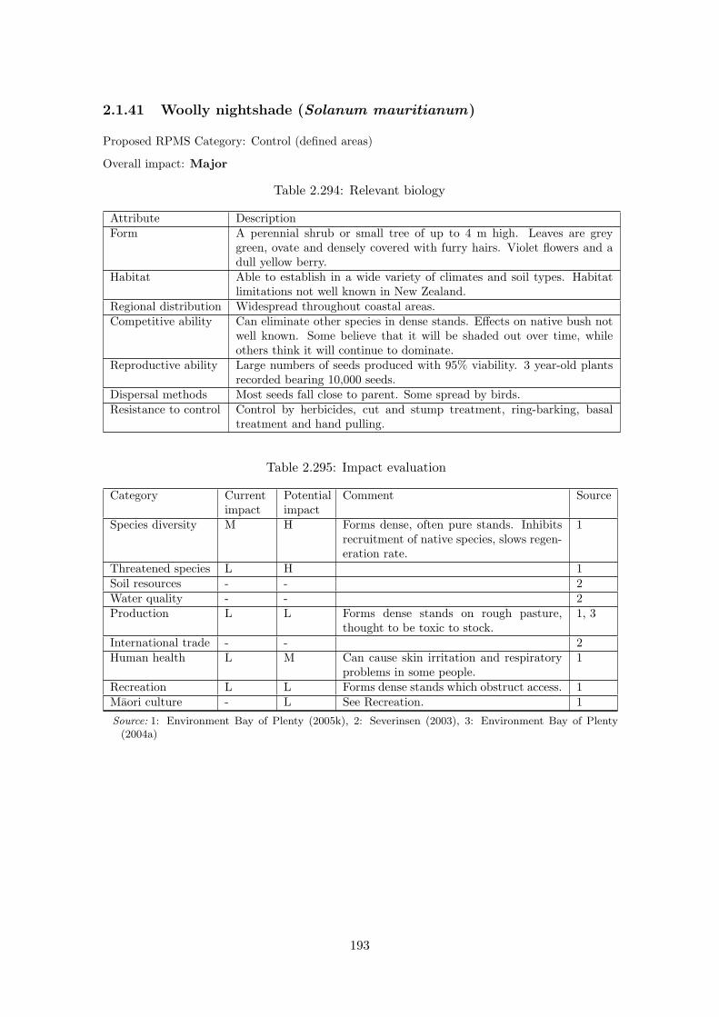
2.1.41 Woolly nightshade (Solanum mauritianum)
Proposed RPMS Category: Control (defined areas)
Overall impact: Major
Table 2.294: Relevant biology
Attribute DescriptionForm A perennial shrub or small tree of up to 4 m high. Leaves are grey
green, ovate and densely covered with furry hairs. Violet flowers and adull yellow berry.
Habitat Able to establish in a wide variety of climates and soil types. Habitatlimitations not well known in New Zealand.
Regional distribution Widespread throughout coastal areas.Competitive ability Can eliminate other species in dense stands. E↵ects on native bush not
well known. Some believe that it will be shaded out over time, whileothers think it will continue to dominate.
Reproductive ability Large numbers of seeds produced with 95% viability. 3 year-old plantsrecorded bearing 10,000 seeds.
Dispersal methods Most seeds fall close to parent. Some spread by birds.Resistance to control Control by herbicides, cut and stump treatment, ring-barking, basal
treatment and hand pulling.
Table 2.295: Impact evaluation
Category Currentimpact
Potentialimpact
Comment Source
Species diversity M H Forms dense, often pure stands. Inhibitsrecruitment of native species, slows regen-eration rate.
1
Threatened species L H 1Soil resources - - 2Water quality - - 2Production L L Forms dense stands on rough pasture,
thought to be toxic to stock.1, 3
International trade - - 2Human health L M Can cause skin irritation and respiratory
problems in some people.1
Recreation L L Forms dense stands which obstruct access. 1Maori culture - L See Recreation. 1Source: 1: Environment Bay of Plenty (2005k), 2: Severinsen (2003), 3: Environment Bay of Plenty
(2004a)
193

Woolly nightshade CBA results
The following are results for cost-benefit analyses for four scenarios, no regional RPMS control,RPMS control as an Exclusion Pest, RPMS control as a Control Pest, and RPMS control as anAdvisory Pest. For the purposes of the CBA calculations, the pest is assumed to continue expandingwith no regional RPMS control, its spread is assumed to be near-arrested under Advisory Controlbut not reduced, and it is assumed to be successfully reduced to the expected smaller extent whenlisted as a Control Pest, more so as an Exclusion pest.
Table 2.296: Woolly nightshade CBA results for four RPMS scenarios, presented as netpresent value (NPV, $) over 50 years. The expenditure refers to regional expenditureunder the RPMS. Minimum and maximum values are in brackets beneath average values.
Scenario Pest impacts Control benefit Expenditure Net benefitNo RPMS 6,577,470 0 0 -6,577,470
(1,726,004–11,428,937) (-1,726,004 – -11,428,937)
Exclusion Pest 166,770 6,410,700 33,733,195 -27,322,495(37,616–273,542) (1,688,388–11,155,395) (-32,044,807 – -22,577,800)
Control Pest 441,454 6,136,016 1,321,216 4,814,800(94,658–766,448) (1,631,346–10,662,489) (310,130 – 9,341,273)
Advisory Pest 204,540 6,372,930 13,212 6,359,718(46,817–329,622) (1,679,187–11,099,315) (1,665,975 – 11,086,103)
Table 2.297: Woolly nightshade CBA base assumptions.
Base assumptions ValuesCurrent area infested (ha) 1,500
Total area potentially infested (ha) 34,500 (34,500–34,500)
Years from naturalisation to total area 25Assessment duration (yr) 50
Weighted average impact per hectare of infested land ($/ha) 26.11 (5.43–46.79)
Any benefits provided by the weed 0Discount rate 0.08
Table 2.298: Woolly nightshade RPMS Exclusion Pest assumptions.
Exclusion Pest assumptions ValuesYears to achieve objectives 9
Final area infested (ha) 187.5 (0–375)
Table 2.299: Woolly nightshade RPMS Control Pest assumptions.
Control Pest assumptions ValuesYears to achieve objectives 50
Final area infested (ha) 938 (750–1,125)
Table 2.300: Woolly nightshade RPMS Advisory Pest assumptions.
Advisory Pest assumptions ValuesYears to achieve objectives 5
194
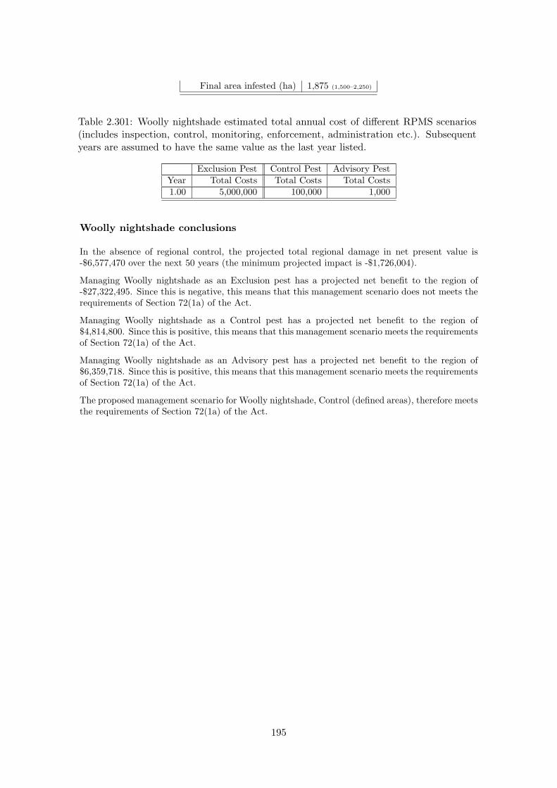
Final area infested (ha) 1,875 (1,500–2,250)
Table 2.301: Woolly nightshade estimated total annual cost of di↵erent RPMS scenarios(includes inspection, control, monitoring, enforcement, administration etc.). Subsequentyears are assumed to have the same value as the last year listed.
Exclusion Pest Control Pest Advisory PestYear Total Costs Total Costs Total Costs1.00 5,000,000 100,000 1,000
Woolly nightshade conclusions
In the absence of regional control, the projected total regional damage in net present value is-$6,577,470 over the next 50 years (the minimum projected impact is -$1,726,004).
Managing Woolly nightshade as an Exclusion pest has a projected net benefit to the region of-$27,322,495. Since this is negative, this means that this management scenario does not meets therequirements of Section 72(1a) of the Act.
Managing Woolly nightshade as a Control pest has a projected net benefit to the region of$4,814,800. Since this is positive, this means that this management scenario meets the requirementsof Section 72(1a) of the Act.
Managing Woolly nightshade as an Advisory pest has a projected net benefit to the region of$6,359,718. Since this is positive, this means that this management scenario meets the requirementsof Section 72(1a) of the Act.
The proposed management scenario for Woolly nightshade, Control (defined areas), therefore meetsthe requirements of Section 72(1a) of the Act.
195

−10 −5 0 5 10 15 20 25
0.0
0.2
0.4
0.6
0.8
1.0
Calibrated logistic growth curve, no RPMS control
Years from present
Prop
ortio
n of
max
imum
ext
ent
Current extent (ha): 1,500
Potential extent (ha): 34,500
Time to potential (yr): 25
Current prop. of potential: 0.043
Figure 2.71: The modelled pest spread until it reaches its anticipated maximum extent.Shown are the results of the average (solid line), minimum (dotted line), and maximum(dashed line) scenarios. (A horizontal line means that the pest has already reached itsmaximum extent.) The vertical dotted-dashed lines indicate the CBA assessment periodused in this report.
196
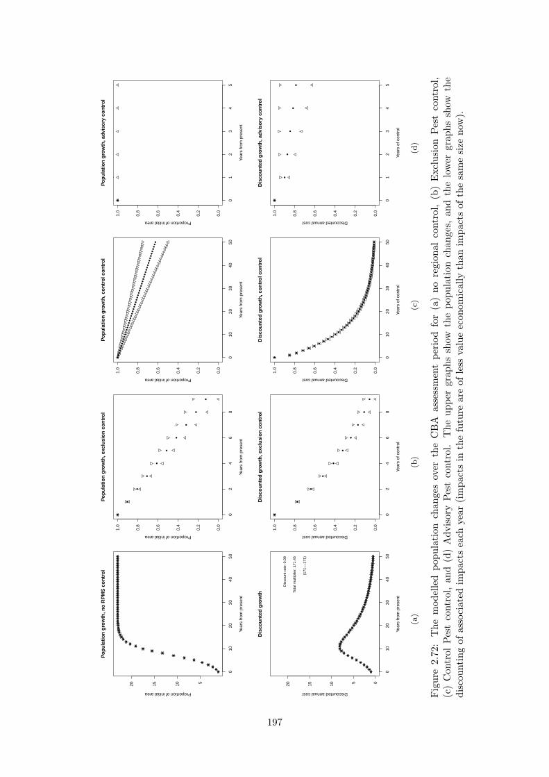
●
●
●
●
●
●
●
●
●
●
●
●
●
●
●●
●●
●●
●●
●●
●●
●●
●●
●●
●●
●●
●●
●●
●●
●●
●●
●●
●●
●
010
2030
4050
5101520
Popu
latio
n gr
owth
, no
RPM
S co
ntro
l
Year
s fro
m p
rese
nt
Proportion of initial area
●●
●
●
●
●
●
●
●
●●
●●
●●
●●
●●
●●
●●
●●
●●
●●
●●
●●
●●
●●
●●
●●
●●
●●
●●
●●
●●
010
2030
4050
05101520
Dis
coun
ted
grow
th
Year
s fro
m p
rese
nt
Discounted annual cost
Dis
coun
t rat
e: 0
.08
Tota
l mul
tiplie
r: 17
1.45
(171−−
171)
(a)
●
●
●
●
●
●
●
●
●
●
02
46
8
0.0
0.2
0.4
0.6
0.8
1.0
Popu
latio
n gr
owth
, exc
lusi
on c
ontro
l
Year
s fro
m p
rese
ntProportion of initial area
●
●
●
●
●
●
●
●
●
●
02
46
8
0.0
0.2
0.4
0.6
0.8
1.0
Dis
coun
ted
grow
th, e
xclu
sion
con
trol
Year
s of
con
trol
Discounted annual cost
(b)
●●
●●
●●
●●
●●
●●
●●
●●
●●
●●
●●
●●
●●
●●
●●
●●
●●
●●
●●
●●
●●
●●
●●
●●
●●
●
010
2030
4050
0.0
0.2
0.4
0.6
0.8
1.0
Popu
latio
n gr
owth
, con
trol c
ontro
l
Year
s fro
m p
rese
nt
Proportion of initial area
●
●
●
●
●
●
●
●
●
●
●
●
●
●
●
●●
●●
●●
●●
●●
●●
●●
●●
●●
●●
●●
●●
●●
●●
●●
●●
●●
●●
010
2030
4050
0.0
0.2
0.4
0.6
0.8
1.0
Dis
coun
ted
grow
th, c
ontro
l con
trol
Year
s of
con
trol
Discounted annual cost
(c)
●
●
●
●
●
●
01
23
45
0.0
0.2
0.4
0.6
0.8
1.0
Popu
latio
n gr
owth
, adv
isor
y co
ntro
l
Year
s fro
m p
rese
nt
Proportion of initial area
●
●
●
●
●
●
01
23
45
0.0
0.2
0.4
0.6
0.8
1.0
Dis
coun
ted
grow
th, a
dvis
ory
cont
rol
Year
s of
con
trol
Discounted annual cost
(d)
Fig
ure
2.72
:T
hem
odel
led
popu
lati
onch
ange
sov
erth
eC
BA
asse
ssm
ent
peri
odfo
r(a
)no
regi
onal
cont
rol,
(b)
Exc
lusi
onPes
tco
ntro
l,(c
)C
ontr
olPes
tco
ntro
l,an
d(d
)A
dvis
ory
Pes
tco
ntro
l.T
heup
per
grap
hssh
owth
epo
pula
tion
chan
ges,
and
the
low
ergr
aphs
show
the
disc
ount
ing
ofas
soci
ated
impa
cts
each
year
(im
pact
sin
the
futu
rear
eof
less
valu
eec
onom
ical
lyth
anim
pact
sof
the
sam
esi
zeno
w).
197

2.1.42 Yellow flag iris (Iris pseudacorus)
Proposed RPMS Category: Control
Overall impact: Major
Table 2.302: Relevant biology
Attribute DescriptionForm Leafy perennial semi-aquatic iris growing up to 2 m. Produces large
yellowish flowers. Rhizomes form dense floating mats. Above groundportions die back if frosted.
Habitat Water plant, growing around margins of ponds, swamps, rivers, water-ways, drains. Tolerant of a wide range of situations including salinity,frost and complete submergence.
Regional distribution Isolated infestations throughout region.Competitive ability Vegetative growth from rhizomes, tall dense growth habit. Has possible
potential to displace virtually all species from the water’s edge margin.Relatively slow rate of spread but now sets viable seed.
Reproductive ability Produces viable seed.Dispersal methods Seeds dispersed by water and wind, sometimes by humans for gardens.Resistance to control Can be adequately controlled with metsulfuron and glyphosate, however
this may damage surrounding plants.
Table 2.303: Impact evaluation
Category Currentimpact
Potentialimpact
Comment Source
Species diversity L M Dense patches and rhizome mats displacenative plants, esp. vulnerable marginalspecies. Poisonous seeds may have impacton birdlife.
1
Threatened species L M 1Soil resources - - 2Water quality L M Can cause flooding and changes in water
levels in swamps.1
Production - L Excludes pasture species. Causes gastro-enteritis in cattle.
3
International trade - - 2Human health - - 2Recreation L H Dense stands obstruct access to estuaries
and waterways.2
Maori culture L M See Recreation. 2Source: 1: Craw (2000), 2: Severinsen (2003), 3: Environment Bay of Plenty (2005l)
198

Yellow flag iris CBA results
The following are results for cost-benefit analyses for four scenarios, no regional RPMS control,RPMS control as an Exclusion Pest, RPMS control as a Control Pest, and RPMS control as anAdvisory Pest. For the purposes of the CBA calculations, the pest is assumed to continue expandingwith no regional RPMS control, its spread is assumed to be near-arrested under Advisory Controlbut not reduced, and it is assumed to be successfully reduced to the expected smaller extent whenlisted as a Control Pest, more so as an Exclusion pest.
Table 2.304: Yellow flag iris CBA results for four RPMS scenarios, presented as net presentvalue (NPV, $) over 50 years. The expenditure refers to regional expenditure under theRPMS. Minimum and maximum values are in brackets beneath average values.
Scenario Pest impacts Control benefit Expenditure Net benefitNo RPMS 71,566 0 0 -71,566
(13,528–356,940) (-13,528 – -356,940)
Exclusion Pest 11 71,555 927,663 -856,108(2–19) (13,526–356,921) (-914,137 – -570,742)
Control Pest 30 71,536 36,333 35,203(6–52) (13,522–356,888) (-22,811 – 320,555)
Advisory Pest 14 71,552 13,212 58,340(3–22) (13,525–356,918) (313 – 343,706)
Table 2.305: Yellow flag iris CBA base assumptions.
Base assumptions ValuesCurrent area infested (ha) 5
Total area potentially infested (ha) 101,447 (34,289–168,604)
Years from naturalisation to total area 100Assessment duration (yr) 50
Weighted average impact per hectare of infested land ($/ha) 0.53 (0.1–0.96)
Any benefits provided by the weed 0Discount rate 0.08
Table 2.306: Yellow flag iris RPMS Exclusion Pest assumptions.
Exclusion Pest assumptions ValuesYears to achieve objectives 9
Final area infested (ha) 0.6 (0–1.2)
Table 2.307: Yellow flag iris RPMS Control Pest assumptions.
Control Pest assumptions ValuesYears to achieve objectives 50
Final area infested (ha) 3 (2–4)
Table 2.308: Yellow flag iris RPMS Advisory Pest assumptions.
Advisory Pest assumptions ValuesYears to achieve objectives 5
Final area infested (ha) 6 (5–8)
199

Table 2.309: Yellow flag iris estimated total annual cost of di↵erent RPMS scenarios(includes inspection, control, monitoring, enforcement, administration etc.). Subsequentyears are assumed to have the same value as the last year listed.
Exclusion Pest Control Pest Advisory PestYear Total Costs Total Costs Total Costs1.00 137,500 2,750 1,000
Yellow flag iris conclusions
In the absence of regional control, the projected total regional damage in net present value is-$71,566 over the next 50 years (the minimum projected impact is -$13,528).
Managing Yellow flag iris as an Exclusion pest has a projected net benefit to the region of -$856,108.Since this is negative, this means that this management scenario does not meets the requirementsof Section 72(1a) of the Act.
Managing Yellow flag iris as a Control pest has a projected net benefit to the region of $35,203.Since this is positive, this means that this management scenario meets the requirements of Section72(1a) of the Act.
Managing Yellow flag iris as an Advisory pest has a projected net benefit to the region of $58,340.Since this is positive, this means that this management scenario meets the requirements of Section72(1a) of the Act.
The proposed management scenario for Yellow flag iris, Control, therefore meets the requirementsof Section 72(1a) of the Act.
200

0 20 40 60 80 100
0.0
0.2
0.4
0.6
0.8
1.0
Calibrated logistic growth curve, no RPMS control
Years from present
Prop
ortio
n of
max
imum
ext
ent
Current extent (ha): 5
Potential extent (ha): 101,447
(34,289−−168,604)
Time to potential (yr): 100
Current prop. of potential: <0.01
Figure 2.73: The modelled pest spread until it reaches its anticipated maximum extent.Shown are the results of the average (solid line), minimum (dotted line), and maximum(dashed line) scenarios. (A horizontal line means that the pest has already reached itsmaximum extent.) The vertical dotted-dashed lines indicate the CBA assessment periodused in this report.
201

●●
●●
●●
●●
●●
●●
●●
●●
●●
●●
●●
●●
●●
●●
●●
●●
●●
●●
●●
●●
●●
●●
●●
●
●
●
●
●
010
2030
4050
0
5000
1000
0
1500
0
Popu
latio
n gr
owth
, no
RPM
S co
ntro
l
Year
s fro
m p
rese
nt
Proportion of initial area
●●
●●
●●
●●
●●
●●
●●
●●
●●
●●
●●
●●
●●
●●
●●
●●
●●
●●
●●
●●
●●
●●
●●
●●
●●
●
010
2030
4050
0
5000
1000
0
1500
0
Dis
coun
ted
grow
th
Year
s fro
m p
rese
nt
Discounted annual cost
Dis
coun
t rat
e: 0
.08
Tota
l mul
tiplie
r: 25
96.8
8
(156
3−−7
681)
(a)
●
●
●
●
●
●
●
●
●
●
02
46
8
0.0
0.2
0.4
0.6
0.8
1.0
Popu
latio
n gr
owth
, exc
lusi
on c
ontro
l
Year
s fro
m p
rese
ntProportion of initial area
●
●
●
●
●
●
●
●
●
●
02
46
8
0.0
0.2
0.4
0.6
0.8
1.0
Dis
coun
ted
grow
th, e
xclu
sion
con
trol
Year
s of
con
trol
Discounted annual cost
(b)
●●
●●
●●
●●
●●
●●
●●
●●
●●
●●
●●
●●
●●
●●
●●
●●
●●
●●
●●
●●
●●
●●
●●
●●
●●
●
010
2030
4050
0.0
0.2
0.4
0.6
0.8
1.0
Popu
latio
n gr
owth
, con
trol c
ontro
l
Year
s fro
m p
rese
nt
Proportion of initial area
●
●
●
●
●
●
●
●
●
●
●
●
●
●
●
●●
●●
●●
●●
●●
●●
●●
●●
●●
●●
●●
●●
●●
●●
●●
●●
●●
●●
010
2030
4050
0.0
0.2
0.4
0.6
0.8
1.0
Dis
coun
ted
grow
th, c
ontro
l con
trol
Year
s of
con
trol
Discounted annual cost
(c)
●
●
●
●
●
●
01
23
45
0.0
0.2
0.4
0.6
0.8
1.0
Popu
latio
n gr
owth
, adv
isor
y co
ntro
l
Year
s fro
m p
rese
nt
Proportion of initial area
●
●
●
●
●
●
01
23
45
0.0
0.2
0.4
0.6
0.8
1.0
Dis
coun
ted
grow
th, a
dvis
ory
cont
rol
Year
s of
con
trol
Discounted annual cost
(d)
Fig
ure
2.74
:T
hem
odel
led
popu
lati
onch
ange
sov
erth
eC
BA
asse
ssm
ent
peri
odfo
r(a
)no
regi
onal
cont
rol,
(b)
Exc
lusi
onPes
tco
ntro
l,(c
)C
ontr
olPes
tco
ntro
l,an
d(d
)A
dvis
ory
Pes
tco
ntro
l.T
heup
per
grap
hssh
owth
epo
pula
tion
chan
ges,
and
the
low
ergr
aphs
show
the
disc
ount
ing
ofas
soci
ated
impa
cts
each
year
(im
pact
sin
the
futu
rear
eof
less
valu
eec
onom
ical
lyth
anim
pact
sof
the
sam
esi
zeno
w).
202

2.1.43 Pest plant beneficiaries and exacerbators
The tables on the following pages identify those in the Bay of Plenty community most likelyto benefit from pest control (“beneficiaries”) and those most likely to exacerbate pest spread orimpacts (“exacerbators”).
203

Tabl
e2.
310:
Ben
efici
arie
sfo
rpe
stpl
ants
Pla
nt
RP
MS
cate
gory
Pas
tora
lH
orti
cult
ure
For
estr
yU
rban
Reg
ional
com
munity
Afr
ican
feat
her
gras
sC
ontr
olM
ajo
rM
inor
Majo
rA
pple
ofSodom
Con
trol
Majo
rM
inor
Asi
atic
knot
wee
dC
ontr
olM
ajo
rB
ones
eed
Con
trol
Majo
rC
hilea
nrh
ubar
bC
ontr
olM
ajo
rC
lim
bin
gsp
indle
ber
ryC
ontr
olM
inor
Majo
rC
oast
tea
tree
Con
trol
Majo
rD
arw
in’s
bar
ber
ryC
ontr
olM
inor
Majo
rE
geri
aden
saC
ontr
ol(d
efined
lake
s)M
ajo
rG
reen
goddes
slily
Con
trol
Majo
rM
ajo
rH
ornw
ort
Con
trol
(defi
ned
lake
s)M
ajo
rIt
alia
nbuck
thor
nC
ontr
olM
inor
Majo
rLag
aros
iphon
Con
trol
(defi
ned
lake
s)M
ajo
rLan
tana
Con
trol
Min
orM
ajo
rLodge
pol
epin
eC
ontr
olM
inor
Min
orM
ajo
rO
ldm
an’s
bea
rdC
ontr
olM
inor
Majo
rR
oyal
fern
Con
trol
Majo
rV
arie
gate
dth
istl
eC
ontr
olM
ajo
rM
inor
Wild
ginge
r(y
ello
wan
dka
hili)
Con
trol
Min
orM
ajo
rW
ild
kiw
ifru
itC
ontr
olM
inor
Majo
rM
ajo
rW
ool
lynig
hts
had
eC
ontr
ol(d
efined
area
s)M
inor
Min
orM
ajo
rM
ajo
rM
ajo
rY
ello
wflag
iris
Con
trol
Majo
r
204

Tabl
e2.
311:
Exa
cerb
ator
sfo
rpe
stpl
ants
Pla
nt
RP
MS
cate
gory
Pas
tora
lH
orti
cult
ure
For
estr
yU
rban
Reg
ional
com
munity
Afr
ican
feat
her
gras
sC
ontr
olM
inor
Min
orA
pple
ofSodom
Con
trol
Min
orA
siat
icknot
wee
dC
ontr
olM
inor
Min
orB
ones
eed
Con
trol
Min
orC
hilea
nrh
ubar
bC
ontr
olM
ajo
rM
inor
Clim
bin
gsp
indle
ber
ryC
ontr
olM
inor
Coa
stte
atr
eeC
ontr
olM
ajo
rM
ajo
rD
arw
in’s
bar
ber
ryC
ontr
olM
inor
Ege
ria
den
saC
ontr
ol(d
efined
lake
s)M
ajo
rG
reen
goddes
slily
Con
trol
Majo
rM
ajo
rH
ornw
ort
Con
trol
(defi
ned
lake
s)M
ajo
rIt
alia
nbuck
thor
nC
ontr
olM
ajo
rM
ajo
rLag
aros
iphon
Con
trol
(defi
ned
lake
s)M
ajo
rLan
tana
Con
trol
Min
orLodge
pol
epin
eC
ontr
olM
inor
Majo
rO
ldm
an’s
bea
rdC
ontr
olM
inor
Majo
rR
oyal
fern
Con
trol
Var
iega
ted
this
tle
Con
trol
Min
orW
ild
ginge
r(y
ello
wan
dka
hili)
Con
trol
Majo
rM
ajo
rW
ild
kiw
ifru
itC
ontr
olM
inor
Majo
rM
inor
Wool
lynig
hts
had
eC
ontr
ol(d
efined
area
s)M
inor
Min
orM
inor
Majo
rY
ello
wflag
iris
Con
trol
Min
orM
ajo
r
205