C-1 Appendix C. Coulomb Fracture Criterion

Our results for the chapters of this thesis use the Hencky-Mises plastic yield

criterion because of its simplicity. We demonstrate with this criterion a bias toward the

stress rate, !!T

, for medium to large heterogeneity ratios, HR , which is a measure of the

magnitude of the spatially heterogeneous stress relative to the spatial mean stress, !!B

.

One question that arises is, do we still see this bias if we use the more common Coulomb

Failure criterion. The answer is yes, but the P-T plots become more complicated because

the two conjugate planes are not perpendicular. Each conjugate plane now has its own

set of P-T axes.

Figure C.1 shows a Mohr circle diagram to visualize our Coulomb Failure. Note,

elsewhere in this thesis, we have used the physics convention that tensile principal

stresses are > 0, and compressive principal stresses are < 0. For this appendix, however,

we will use the opposite convention: tensile principal stresses are < 0, and compressive

principal stresses are > 0, which is the common convention when working with Mohr’s

circles. Therefore in Figure C.1, !1 is our most compressive principal stress, and !

3 is

the least compressive principal stress. ! is the shear stress axis, !n

is the normal stress

axis, and the line elevated at angle ! represents the failure threshold for Coulomb

Failure. The value, !0, represents any cohesion in the material. In our simulations, we

want to generate fresh fractures; therefore, for Coulomb Failure, we solve for where the

circle (representing the outer set of shear stress/normal stress values) is tangent to the

failure threshold. Last, the angle ! represents the angle between the failure plane and the

most compressive principal stress, !1.

C-2

Figure C.1. Mohr circle and Coulomb Failure Criterion. On the axes of shear stress,

! , vs. normal stress, !n

, the principal stresses, !1 (most compressive principal stress)

and !3 (least compressive principal stress), define the Mohr’s circle. The outside

circumference of the Mohr’s circle shown specifies the set of ! , !n

values for all

orientations of planes whose normals lie in the plane of !1 and !

3. The line elevated at

an angle, ! , specifies the failure threshold for the Coulomb Failure Criterion, where

µ = tan! , and !0 is the cohesion of the material. Failure thus occurs where the line is

tangent to the plane. In our simulations of Coulomb Failure, we solve for the time, t ,

when the Mohr circle becomes tangent to the failure line. Once failure occurs, !

describes the angle between the failure planes and !1. For µ = 0.0 , ! = 45° and the

conjugate failure planes are perpendicular. This is the same as the maximally oriented

planes we calculate in our plastic yield criterion. For µ > 0.0 we find ! < 45° . In

addition, the conjugate failure planes are no longer perpendicular, resulting in two sets

of P-T axes per failure (Figure C.3).

C-3 The coefficient of friction, µ , is defined as

µ = tan!; (C.1)

therefore, the failure threshold can be described with the following equation,

! = !0+ µ"

n. (C.2)

The Mohr circle can be described with,

!n" !

C( )2

+ #2= r

2 (C.3)

where the center point is

!C=!1+!

3

2 (C.4)

and the radius is

r =!1" !

3

2 . (C.5)

Substituting Equations (C.4) and (C.5) into Equation (C.3) we have the following

description of the Mohr circles:

!n"!1+!

3

2

#$%

&'(2

+ ) 2 =!1" !

3

2

#$%

&'(2

. (C.6)

If we solve for ! we have,

! = ± "n"1+"

3( ) # " n

2# "

1"3

(C.7)

where the positive solution represents the top half of the Mohr circle and the negative

solution represents the bottom half of the Mohr circle.

The two failure planes are ±! relative to the !1 axes, so if we solve for one

failure plane we know the other. Let us set the positive solution of Equation (C.7) equal

C-4 to ! = !

0+ µ"

n so that the Mohr circle is tangent to the failure line, and then solve for

the normal stress, !n

, at this failure point,

!n=

!1+!

3" 2#

0µ( ) ± !

1+!

3" 2#

0µ( )

2

" 4 µ2 +1( ) # 02 +!1!3( )

2 µ2 +1( ) . (C.8)

We want solutions where ! += !

" or !n

+= !

n

" ; therefore, we want the + and !

solutions to Equation (C.8) to equal one another. This means that the second quantity in

the numerator should equal zero,

!1+!

3" 2#

0µ( )

2

" 4 µ2 +1( ) # 02 +!1!3( ) = 0. (C.9)

Solving for !1 in terms of !

3,

!1= 1+ 2µ2( )! 3

+ 2"0µ ± 2 1+ µ2( ) µ!

3+ "

0( ). (C.10)

We want !1 to increase when !

3 increases; thus, we choose the positive root to give the

final equation for the relation between !1 and !

3,

!1= 1+ 2µ2 + 2µ 1+ µ2( )"#$

%&'!3+ 2 µ + 1+ µ2( )"

#$%&'(0. (C.11)

One of our first questions about this equation is, over what range of values is it

valid. We find that it is valid for !3> "

#0

µ; specifically, the least compressive principal

stress, !3, must be greater than the intercept with the !

n axis at ! = 0.0 .

Of interest, when we solve Equation (C.11) in terms of the cohesion, !0,

!0="1# 1+ 2µ2 + 2µ 1+ µ2( )$%&

'()"3

2 µ + 1+ µ2( )$%&

'()

(C.12)

C-5 and set the coefficient of friction to zero, µ = 0.0 , we find that

!0="

1# "

3

2 for µ = 0.0, (C.13)

and that Equation (C.2) becomes

! ="

1# "

3

2 for µ = 0.0, (C.14)

which is similar to our plastic yield criterion. Equation (C.14) indicates that when

µ = 0.0 , the failure threshold is independent of pressure, p . It is a straight line at

! = !0, the cohesion of the material. Failure occurs when the deviatoric part of the stress

matrix, !1" !

3

2, is equal to !

0. If !

0 in the Coulomb Failure Criterion is given the same

value as !0 in the plastic yield criterion, and µ is set equal to zero, the two

methodologies should produce similar answers. Of course, if µ > 0.0 , such as µ = 0.6 ,

the results for Coulomb Failure will become more complicated as shown in Figure C.3.

For our simulations of Coulomb Failure, we create random heterogeneous

principal stresses, !1, !

2, and !

3, and random orientations ! , ",#[ ]( ) , as described in

Chapter 3. We scale the pressure, p , to the desired level, add a background stress, !B

,

set the cohesion, !0, so the failure threshold will be close to Mohr circles for our points,

then bring points to failure by applying a tectonic stress rate, !!T

. For the Coulomb

Failure Criterion, failure is determined by looking at the ratio of principal stresses; hence,

the failure criterion no longer uses an invariant quantity to determine failure, independent

of coordinate system. The methodology involves adding an increment of stress, using the

stress rate, !!T

, recalculating the principal stresses, checking for failure, adding another

increment of stress, etc.

C-6 Figures C.2 and C.3 show the results of some of our calculations. Our

heterogeneous stress in these calculations has ! = 0.0 . The background stress added is

!B2

, the background stress for our “Southern San Andreas Fault” simulations from

Chapter 4. We plot three different heterogeneity ratios for Figures C.2 and C.3,

HR = 0.1, 1.0, and 10 . In all the P-T axes plots for Figures C.2 and C.3, we show the

first 1,000 failures using the Coulomb Fracture Criterion for a grid of 100,001 points.

On the left column in Figure C.2, we have µ = 0.0 and Pressure Ratio = 0.0 .

This should produce results similar to our plastic yield criterion, and indeed it does. The

heterogeneous scatter of the P-T axes increases with increasing HR , and there is an

average rotation of the P-T axes orientations with increasing HR , a rotation toward the

stress rate tensor, !!T

. On the right column in Figure C.2, we show P-T plots for µ = 0.0

and Pressure Ratio = 1.0 . A Pressure Ratio = 1.0 means that

Mean Pressure( )

Mean Spatially Heterogeneous !I2( )

= 1.0 . Adding this amount of pressure in our

simulations has little to no effect. It may reduce the scatter of the P-T axes a small

amount, but again there is still the increasing bias toward the stress rate tensor, !!T

, as

HR increases.

The left column of Figure C.3 is the same as the right column in Figure C.2, P-T

plots for ! = 0.0 , µ = 0.0 , and Pressure Ratio = 1.0 . The right column changes the

coefficient of friction to µ = 0.6 . We randomly choose between the two possible

conjugate planes and plot their corresponding P-T axes. Since the conjugate planes are

no longer perpendicular, there is a bifurcation of the P-T axes that is especially evident

for HR = 0.1 in the top row. As HR increases, the scatter due to the heterogeneity

C-7 begins to connect these two separate clusters of P-T axes as seen for HR = 1.0 in the

middle row. Then as HR increases to HR = 10.0 , the P-T axes are so scattered it is

difficult to distinguish any pattern. In general, even for µ = 0.6 , Coulomb Fracture, we

see both of the effects observed in the plastic criterion for increasing HR : 1) Increasing

scatter of the P-T axes and 2) Increasing bias toward the stress rate, !!T

. The two sets of

P-T axes for µ = 0.6 simply complicate the results; thus why we use the plastic yield

criterion for the rest of the simulations in this thesis.

C-8

C-9 Figure C.2. Results from our Coulomb Fracture simulations. P-T axes for the first

1,000 failures from a 100,001 point grid with ! = 0.0 and µ = 0.0 . On the left, no

pressure has been added to the deviatoric stress in the simulations; on the right, pressure

was added so that the Pressure Ratio = 1.0 . The top row compares the two sets of

simulations for HR = 0.1 , the middle row, HR = 1.0 , and the bottom row, HR = 10.0 .

We find that with and without pressure, the Coulomb Failure simulations replicate two

features of our plastic yield simulations: 1) Increasing P-T scatter with increasing HR

and 2) Increasing bias toward the stress rate tensor, !!T

, with increasing HR , where the

!!T

has N-S compression and E-W tension.

C-10

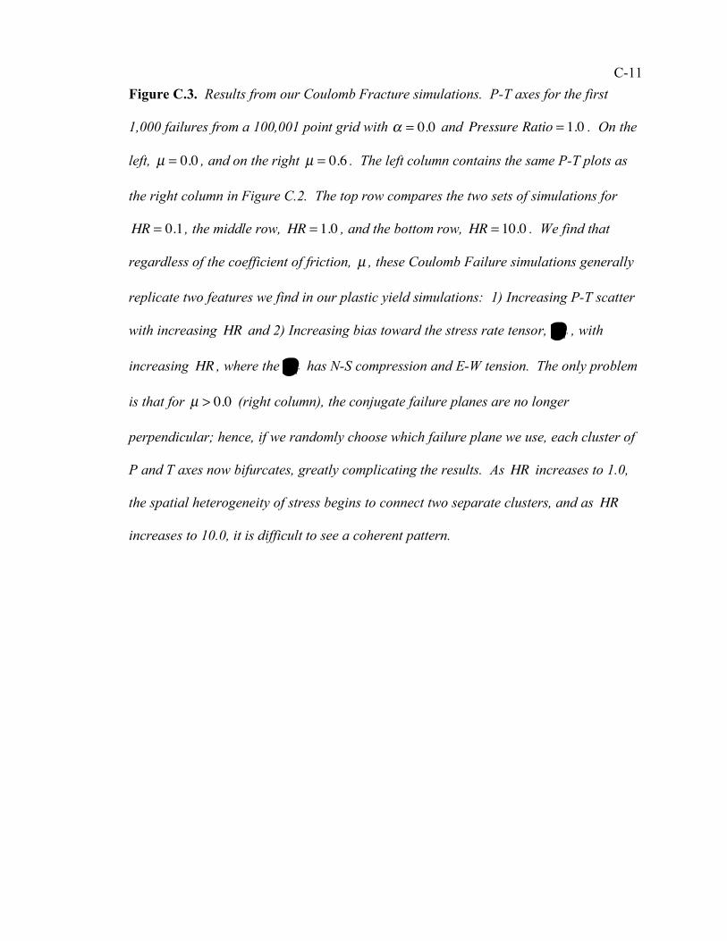
C-11 Figure C.3. Results from our Coulomb Fracture simulations. P-T axes for the first

1,000 failures from a 100,001 point grid with ! = 0.0 and Pressure Ratio = 1.0 . On the

left, µ = 0.0 , and on the right µ = 0.6 . The left column contains the same P-T plots as

the right column in Figure C.2. The top row compares the two sets of simulations for

HR = 0.1 , the middle row, HR = 1.0 , and the bottom row, HR = 10.0 . We find that

regardless of the coefficient of friction, µ , these Coulomb Failure simulations generally

replicate two features we find in our plastic yield simulations: 1) Increasing P-T scatter

with increasing HR and 2) Increasing bias toward the stress rate tensor, !!T

, with

increasing HR , where the !!T

has N-S compression and E-W tension. The only problem

is that for µ > 0.0 (right column), the conjugate failure planes are no longer

perpendicular; hence, if we randomly choose which failure plane we use, each cluster of

P and T axes now bifurcates, greatly complicating the results. As HR increases to 1.0,

the spatial heterogeneity of stress begins to connect two separate clusters, and as HR

increases to 10.0, it is difficult to see a coherent pattern.