Embed Size (px)
Citation preview
Appendix AThe MIDAS Data Reduction
A Short Story
We build our measuring instruments by ourselves, but the costs for variouscomponents are always a problem. Who has a thousand Euros ready to go for ahighly efficient grating? You ask colleagues if they have a mirror mount for you orcan provide a cheap slit. An impossible situation! Eventually we needed a new partfor our spectrograph. We called a manufacturer and were connected to a low-ranktechnician who wasn’t too helpful. Mutual understanding among professionals ishigh, and we now share our various experiences. We “whine” about our financialsuffering and describe our technical needs. On the other hand, we hear things like“I have here a large grating in storage that we don’t need anymore. I can send it toyou. . . ” Hence, our scrounging was highly successful and we refer to such requestsas “High level begging”.
A.1 The MIDAS Environment
The astronomical data reduction packages MIDAS and IRAF both supply allnecessary steps for high quality data reduction. They are complex and requireextensive training. However, the respective user manuals are not easy to understandso that the average novice in a research institute can not easily get started. Mostupcoming researchers benefit from the “generation contract” within the community.The more experienced help the beginners and, hence, within an institute someoneis always approachable for questions. It is not our intention to discuss all detailedreduction tasks. At this point we only want to deliver the main and most importantparts for the very first steps in MIDAS (the IRAF structure is somewhat different butequivalent) and want to give a very first impression of its command structure, somecommands and steps. For program details we refer to the MIDAS user manual.
© Springer-Verlag Berlin Heidelberg 2015T. Eversberg, K. Vollmann, Spectroscopic Instrumentation, Springer Praxis Books,DOI 10.1007/978-3-662-44535-8
561
562 A The MIDAS Data Reduction
Working with MIDAS requires some adjustment by the majority of (Windows)users, and they need to get used to the different working steps in the UNIXenvironment. After learning the first steps, MIDAS is very comfortable to workwith and one quickly gets reliable results. First, we give a quick overview aboutwhat MIDAS is and how it works, and then we describe some details of differentreduction steps.
ESO-MIDAS has already been developed in the 1980s and quickly becameone of the main tools for astronomical image and data processing in UNIXoperating system environments. It is fully interactive and can perform user-definedprocedures and algorithms. It has a modular design so that it can be adapted todifferent environments.1 It can be ported to different machines, works with standardlanguages such as FORTRAN and C, and can handle the XWindow system. Itcan be programmed via simple interface routines and its code is open source foreasy implementation of new software. The basic structure consists of several parts.For instance, it permits a backup of all historical operation commands during onesession. Additional applications can be made via the corresponding interfaces forFORTRAN77, C procedures and for the MIDAS Control Language (MCL). Theseare ordered in different parts according to their importance. The main areas are coreapplications like “Image and Graphic Display”, general image processing, “TableFile System”, a “Fitting Package” to process non-linear functions and Data I/O(Input/Output) for data transfer to other storage media. MIDAS procedures can bewritten in MCL and be grouped in so-called “jobs”, without having to recompilethe program. The “MCL Debugger” enables error fixing in the source code. In thischapter we demonstrate a simplified MIDAS reduction procedure for spectroscopicdata, based on a tutorial by Günter Gebhard. We want to emphasize that the stepspresented here only reflect a small selection of all MIDAS procedures and we referto the corresponding MIDAS User Manual.
A.1.1 Nomenclatura
MIDAS expects all image recordings in fits format, the standard file format used inastronomy and of CCD software on the market. Images and graphics are imaged inseparate displays. Internally MIDAS treats images and tables in the specific formats*.bdf and *.tbl, respectively, which can be converted into appropriate fits formatsat any time for use outside MIDAS. MIDAS has specific packages, the so-called“contexts” for various applications and ESO instruments. The contexts can be easilyadapted to other instrumentation, off-the-shelf or not.
To describe the MIDAS procedures, we write all MIDAS commands in uppercaseand all parameters as well as image and file names in italics. MIDAS commands
1This includes UNIX emulation in Windows using virtual machines, e.g., VMware.
A.1 The MIDAS Environment 563
always consist of two parts, the COMMAND/QUALIFIER. For instance, thecommandOVERPLOT/SYMBOL 15 4108,0.5 2.0
draws an upward pointing arrow in the graphics window at the coordinates x D4108, y D 0.5 in double size.
One can either write the full COMMAND/QUALIFIER command or use thefirst three letters. OVE/SYM is the same as OVERPLOT/SYMBOL. MIDASdistinguishes uppercase and lowercase letters for files but not for commands. Forclarity, here we write MIDAS commands always in uppercase letters and the monitoroutput in bold face.
A.1.2 Start, Help and End
We start MIDAS in an xterm window with the command >Inmidas. With “help” wecan call descriptive help texts. We end MIDAS again with “bye” and go back tothe UNIX/Linux shell. When starting MIDAS, a directory “midwork” is created inwhich the login.prg file is executed, if it is there. login.prg contains optional MIDAScommands that are executed immediately when MIDAS starts.
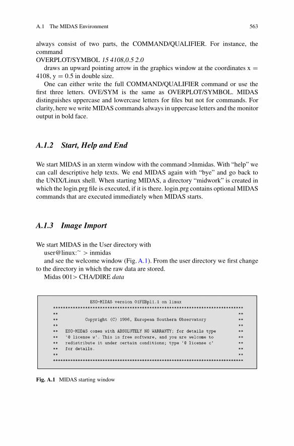
A.1.3 Image Import
We start MIDAS in the User directory withuser@linux:� > inmidasand see the welcome window (Fig. A.1). From the user directory we first change
to the directory in which the raw data are stored.Midas 001> CHA/DIRE data
Fig. A.1 MIDAS starting window
564 A The MIDAS Data Reduction
We are now in the data directory, but MIDAS does not reveal this by itself. Weneed to request this information with the UNIX command pwd (present workingdirectory). MIDAS only understands UNIX commands with a dollar prefix.
Midas 002> $ pwd/home/user/DatenThe directory content can also be called with the corresponding LINUX com-
mand.Midas 003> $ lscflat.fts dark0020.fts dark0014.fts neon1.fts rigel.fts sir1.fts re0317.fts
bias.ftsThe listed images are
cflat.fts CCD flat fielddark0020.fts Dark with 20s exposure timedark0014.fts Dark with 14s exposure timeneon1.fts Neon lamprigel.fts Spectrum of Rigelsir1.fts Spectrum of Siriusstar1.fts Spectrum of another starbias.fts Bias field
Note that these data are only example images we use for explanation. Toactively follow our steps it is necessary to have such calibration and stellar data(not necessarily Rigel and Sirius) available. We first work with the two imagesstar1.fts and the corresponding dark field d0020.fts. Both are stored in a self-createddirectory, e.g., /home/user/data. First, we want to look at some pictures. We firstopen a display
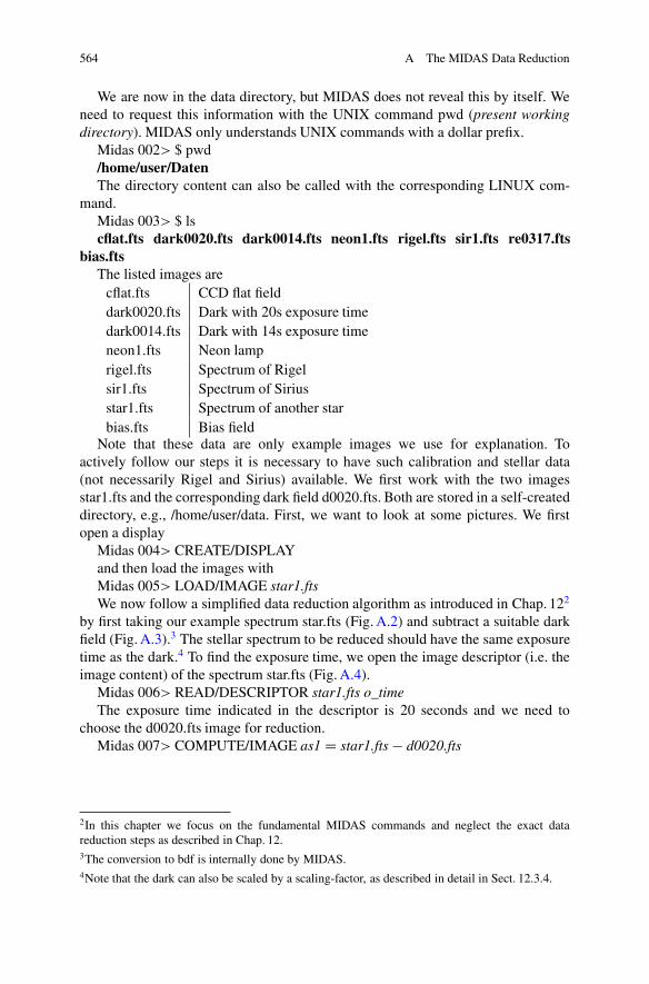
Midas 004> CREATE/DISPLAYand then load the images withMidas 005> LOAD/IMAGE star1.ftsWe now follow a simplified data reduction algorithm as introduced in Chap. 122
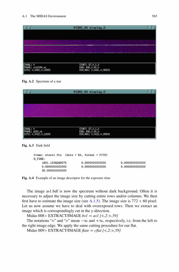
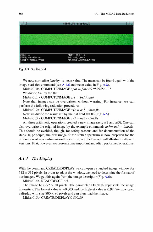
by first taking our example spectrum star.fts (Fig. A.2) and subtract a suitable darkfield (Fig. A.3).3 The stellar spectrum to be reduced should have the same exposuretime as the dark.4 To find the exposure time, we open the image descriptor (i.e. theimage content) of the spectrum star.fts (Fig. A.4).
Midas 006> READ/DESCRIPTOR star1.fts o_timeThe exposure time indicated in the descriptor is 20 seconds and we need to
choose the d0020.fts image for reduction.Midas 007> COMPUTE/IMAGE as1 D star1.fts � d0020.fts
2In this chapter we focus on the fundamental MIDAS commands and neglect the exact datareduction steps as described in Chap. 12.3The conversion to bdf is internally done by MIDAS.4Note that the dark can also be scaled by a scaling-factor, as described in detail in Sect. 12.3.4.
A.1 The MIDAS Environment 565
Fig. A.2 Spectrum of a star
Fig. A.3 Dark field
Fig. A.4 Example of an image descriptor for the exposure time
The image as1.bdf is now the spectrum without dark background. Often it isnecessary to adjust the image size by cutting entire rows and/or columns. We thenfirst have to estimate the image size (see A.1.5). The image size is 772 � 60 pixel.Let us now assume we have to deal with overexposed rows. Then we extract animage which is correspondingly cut in the y-direction.
Midas 008> EXTRACT/IMAGE bs1 D as1 [<,2:>,59]The notations “<” and “>” mean �1 and C1, respectively, i.e. from the left to
the right image edge. We apply the same cutting procedure for our flat.Midas 009> EXTRACT/IMAGE flate D cflat [<,2:>,59]
566 A The MIDAS Data Reduction
Fig. A.5 Our flat field
We now normalize flate by its mean value. The mean can be found again with theimage statistics command (see A.1.6 and mean value in Fig. A.8).
Midas 010> COMPUTE/IMAGE nflat D flate / 9.987945e�01We divide bs1 by the flat.Midas 011> COMPUTE/IMAGE cs1 D bs1 / nflatNote that images can be overwritten without warning. For instance, we can
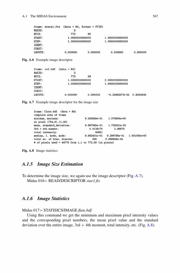
perform the following reduction procedure:Midas 012> COMPUTE/IMAGE as2 D as1 � bias.ftsNow we divide the result as2 by the flat field flat.fts (Fig. A.5).Midas 013> COMPUTE/IMAGE as3 D as2 / nflat.ftsAll three arithmetic operations created a new image (as1, as2 and as3). One can
also overwrite the original image by the example commands as1D as1 � bias.fts.This should be avoided, though, for safety reasons and for documentation of thesteps. In principle, the raw image of the stellar spectrum is now prepared for theproduction of a one-dimensional spectrum, and below we will illustrate differentversions. First, however, we present some important and often performed operations.
A.1.4 The Display
With the command CREATE/DISPLAY we can open a standard image window for512 � 512 pixels. In order to adapt the window, we need to determine the format ofour images. We get this again from the image descriptor (Fig. A.6).
Midas 014> READ/DESCR cs1The image has 772 � 58 pixels. The parameter LHCUTS represents the image
intensities. The lowest value is �0.003 and the highest value is 0.92. We now opena display with size 800 � 80 pixels and can then load the image.
Midas 015> CREATE/DISPLAY 0 800,80
A.1 The MIDAS Environment 567
Fig. A.6 Example image descriptor
Fig. A.7 Example image descriptor for the image size
Fig. A.8 Image statistics
A.1.5 Image Size Estimation
To determine the image size, we again use the image descriptor (Fig. A.7).Midas 016> READ/DESCRIPTOR star1.fts
A.1.6 Image Statistics
Midas 017> STATISICS/IMAGE flate.bdfUsing this command we get the minimum and maximum pixel intensity values
and the corresponding pixel numbers, the mean pixel value and the standarddeviation over the entire image, 3rd C 4th moment, total intensity, etc. (Fig. A.8).
568 A The MIDAS Data Reduction
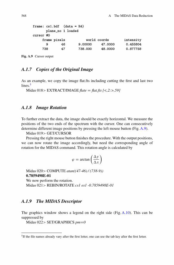
Fig. A.9 Cursor output
A.1.7 Copies of the Original Image
As an example, we copy the image flat.fts including cutting the first and last twolines.5
Midas 018> EXTRACT/IMAGE flate D flat.fts [<,2:>,59]
A.1.8 Image Rotation
To further extract the data, the image should be exactly horizontal. We measure thepositions of the two ends of the spectrum with the cursor. One can consecutivelydetermine different image positions by pressing the left mouse button (Fig. A.9).
Midas 019> GET/CURSORPressing the right mouse button finishes the procedure. With the output positions,
we can now rotate the image accordingly, but need the corresponding angle ofrotation for the MIDAS command. This rotation angle is calculated by
' D arctan
��y
�x
�
Midas 020> COMPUTE atan((47-46) / (738-9))0.7859498E-01We now perform the rotation.Midas 021> REBIN/ROTATE cs1 es1 -0.7859498E-01
A.1.9 The MIDAS Descriptor
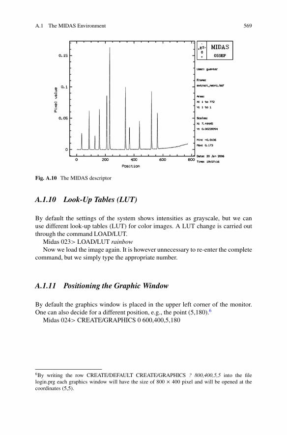
The graphics window shows a legend on the right side (Fig. A.10). This can besuppressed by
Midas 022> SET/GRAPHICS pmD0
5If the file names already vary after the first letter, one can use the tab key after the first letter.
A.1 The MIDAS Environment 569
Fig. A.10 The MIDAS descriptor
A.1.10 Look-Up Tables (LUT)
By default the settings of the system shows intensities as grayscale, but we canuse different look-up tables (LUT) for color images. A LUT change is carried outthrough the command LOAD/LUT.
Midas 023> LOAD/LUT rainbowNow we load the image again. It is however unnecessary to re-enter the complete
command, but we simply type the appropriate number.
A.1.11 Positioning the Graphic Window
By default the graphics window is placed in the upper left corner of the monitor.One can also decide for a different position, e.g., the point (5,180).6
Midas 024> CREATE/GRAPHICS 0 600,400,5,180
6By writing the row CREATE/DEFAULT CREATE/GRAPHICS ? 800,400,5,5 into the filelogin.prg each graphics window will have the size of 800 � 400 pixel and will be opened at thecoordinates (5,5).
570 A The MIDAS Data Reduction
A.2 Spectrum Extraction
A.2.1 AVERAGE/ROW
Before we reduce the two-dimensional image to a one-dimensional spectrum weneed to be sure that the image contains only the stellar information. Since ouralgorithm only eliminated instrument interference, introduced by the instrument(flat field) and the CCD camera (dark and bias field), the sky background or scatteredlight are still present in the image data. Both, however, must be eliminated. We selecttwo image regions next to the spectrum. We determine the intensities of differentpixels or even better the average value of all pixels and then subtract it from theentire image. Our spectrum is positioned approximately on the line 47 and the regionbetween the corners (2,2) and (770,40) (Fig. A.11) as well as (2,54) and (770,59)(Fig. A.12) should contain only noise.
Midas 025> STATISTICS/IMAGE es1 [2,2:770,40]Midas 026> STATISTICS/IMAGE es1 [2,54:770,59]It is now important not to calculate the average of all pixel values, but the median,
because extreme deviations such as cosmic rays and hot pixels are then sorted out.Such pixels would otherwise seriously affect the mean and distort the results. In ourexample, the median is only 0.0006 and is almost negligible.
Midas 027> COMPUTE/IMAGE gs1 D es1 � 0.0006The spectral signal on the chip must now be collapsed perpendicular to the
dispersion direction to a 1D spectrum. To visualize the pixel boundaries for
Fig. A.11 Image statistics for the region [2,2:770,40]
Fig. A.12 Image statistics for the region [2,2:770,40]
A.2 Spectrum Extraction 571
Fig. A.13 Column plot perpendicular to the dispersion direction
Fig. A.14 Collapsed 1D spectrum
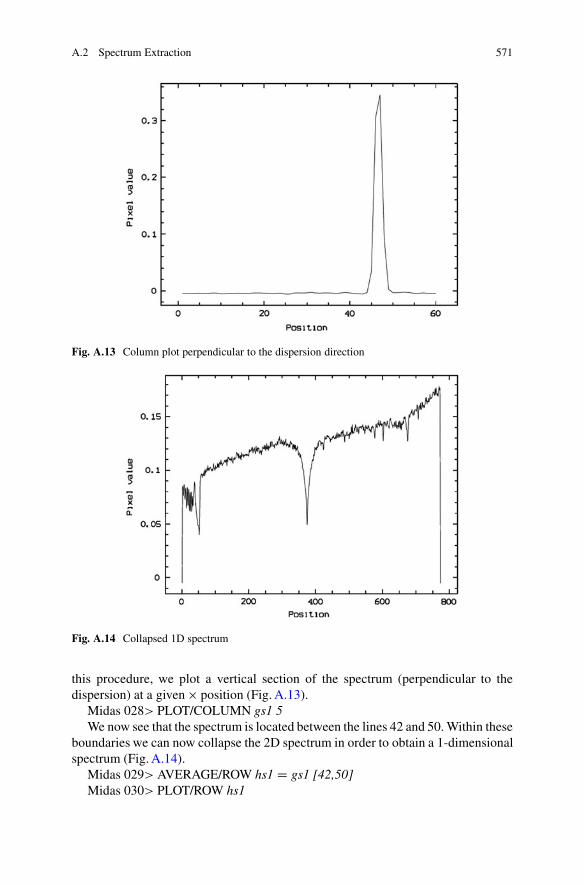
this procedure, we plot a vertical section of the spectrum (perpendicular to thedispersion) at a given � position (Fig. A.13).
Midas 028> PLOT/COLUMN gs1 5We now see that the spectrum is located between the lines 42 and 50. Within these
boundaries we can now collapse the 2D spectrum in order to obtain a 1-dimensionalspectrum (Fig. A.14).
Midas 029> AVERAGE/ROW hs1 D gs1 [42,50]Midas 030> PLOT/ROW hs1
572 A The MIDAS Data Reduction
Fig. A.15 Flipped image of Fig. A.14
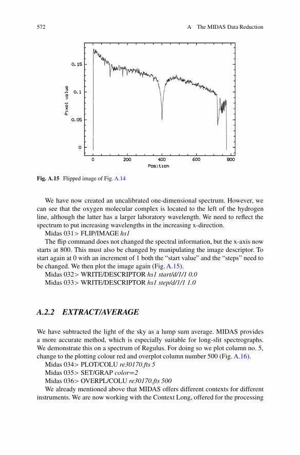
We have now created an uncalibrated one-dimensional spectrum. However, wecan see that the oxygen molecular complex is located to the left of the hydrogenline, although the latter has a larger laboratory wavelength. We need to reflect thespectrum to put increasing wavelengths in the increasing x-direction.
Midas 031> FLIP/IMAGE hs1The flip command does not changed the spectral information, but the x-axis now
starts at 800. This must also be changed by manipulating the image descriptor. Tostart again at 0 with an increment of 1 both the “start value” and the “steps” need tobe changed. We then plot the image again (Fig. A.15).
Midas 032> WRITE/DESCRIPTOR hs1 start/d/1/1 0.0Midas 033> WRITE/DESCRIPTOR hs1 step/d/1/1 1.0
A.2.2 EXTRACT/AVERAGE
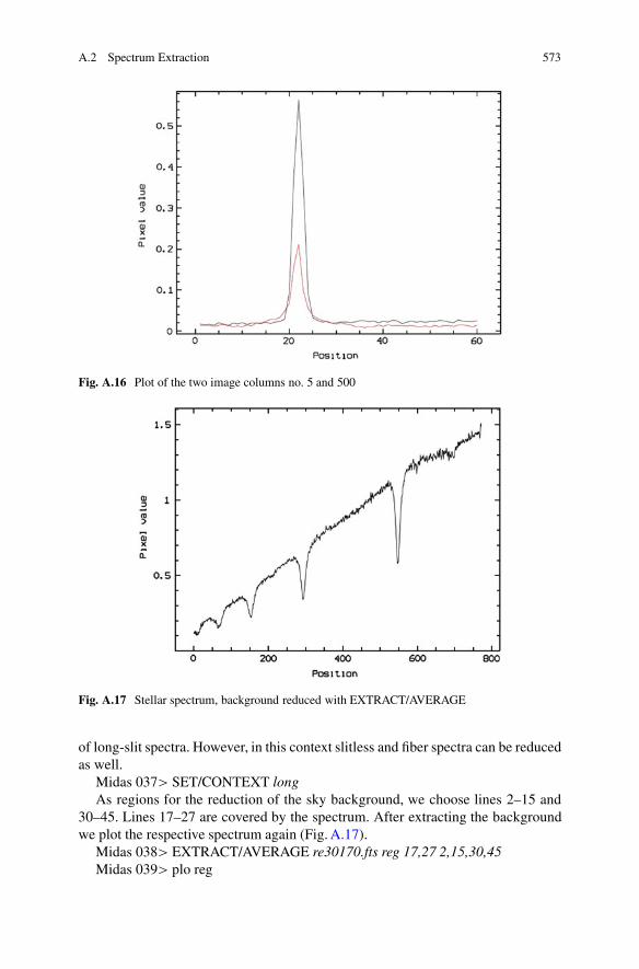
We have subtracted the light of the sky as a lump sum average. MIDAS providesa more accurate method, which is especially suitable for long-slit spectrographs.We demonstrate this on a spectrum of Regulus. For doing so we plot column no. 5,change to the plotting colour red and overplot column number 500 (Fig. A.16).
Midas 034> PLOT/COLU re30170.fts 5Midas 035> SET/GRAP colorD2Midas 036> OVERPL/COLU re30170.fts 500We already mentioned above that MIDAS offers different contexts for different
instruments. We are now working with the Context Long, offered for the processing
A.2 Spectrum Extraction 573
Fig. A.16 Plot of the two image columns no. 5 and 500
Fig. A.17 Stellar spectrum, background reduced with EXTRACT/AVERAGE
of long-slit spectra. However, in this context slitless and fiber spectra can be reducedas well.
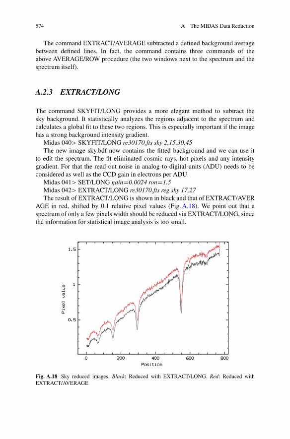
Midas 037> SET/CONTEXT longAs regions for the reduction of the sky background, we choose lines 2–15 and
30–45. Lines 17–27 are covered by the spectrum. After extracting the backgroundwe plot the respective spectrum again (Fig. A.17).
Midas 038> EXTRACT/AVERAGE re30170.fts reg 17,27 2,15,30,45Midas 039> plo reg
574 A The MIDAS Data Reduction
The command EXTRACT/AVERAGE subtracted a defined background averagebetween defined lines. In fact, the command contains three commands of theabove AVERAGE/ROW procedure (the two windows next to the spectrum and thespectrum itself).
A.2.3 EXTRACT/LONG
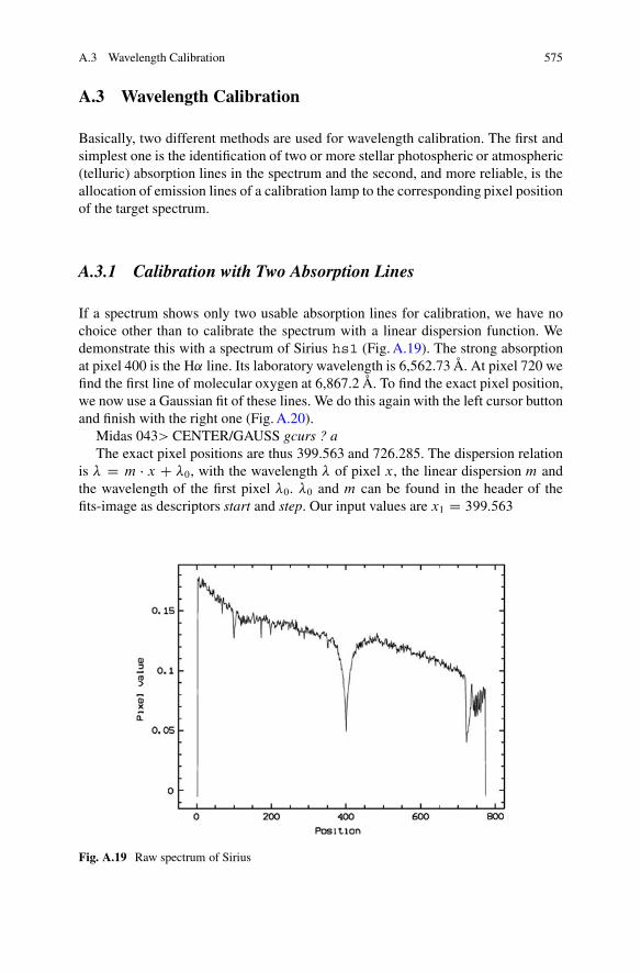
The command SKYFIT/LONG provides a more elegant method to subtract thesky background. It statistically analyzes the regions adjacent to the spectrum andcalculates a global fit to these two regions. This is especially important if the imagehas a strong background intensity gradient.
Midas 040> SKYFIT/LONG re30170.fts sky 2,15,30,45The new image sky.bdf now contains the fitted background and we can use it
to edit the spectrum. The fit eliminated cosmic rays, hot pixels and any intensitygradient. For that the read-out noise in analog-to-digital-units (ADU) needs to beconsidered as well as the CCD gain in electrons per ADU.
Midas 041> SET/LONG gainD0.0024 ronD1.5Midas 042> EXTRACT/LONG re30170.fts reg sky 17,27The result of EXTRACT/LONG is shown in black and that of EXTRACT/AVER
AGE in red, shifted by 0.1 relative pixel values (Fig. A.18). We point out that aspectrum of only a few pixels width should be reduced via EXTRACT/LONG, sincethe information for statistical image analysis is too small.
Fig. A.18 Sky reduced images. Black: Reduced with EXTRACT/LONG. Red: Reduced withEXTRACT/AVERAGE
A.3 Wavelength Calibration 575
A.3 Wavelength Calibration
Basically, two different methods are used for wavelength calibration. The first andsimplest one is the identification of two or more stellar photospheric or atmospheric(telluric) absorption lines in the spectrum and the second, and more reliable, is theallocation of emission lines of a calibration lamp to the corresponding pixel positionof the target spectrum.
A.3.1 Calibration with Two Absorption Lines
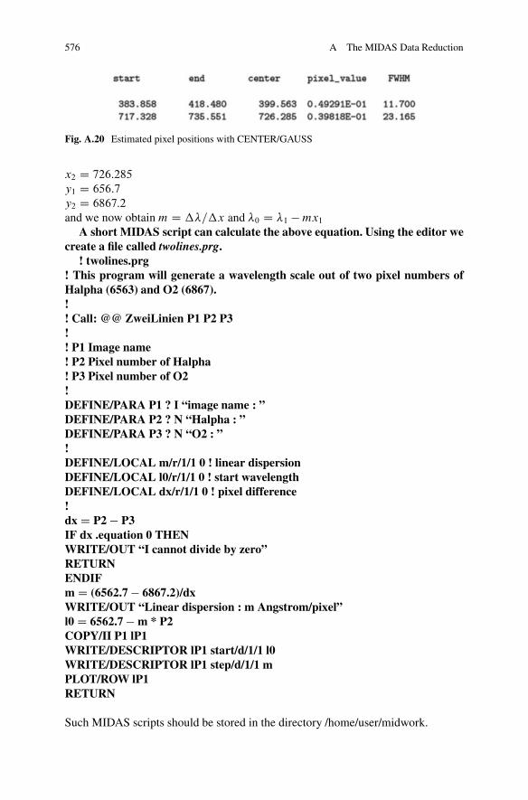
If a spectrum shows only two usable absorption lines for calibration, we have nochoice other than to calibrate the spectrum with a linear dispersion function. Wedemonstrate this with a spectrum of Sirius hs1 (Fig. A.19). The strong absorptionat pixel 400 is the H˛ line. Its laboratory wavelength is 6,562.73 Å. At pixel 720 wefind the first line of molecular oxygen at 6,867.2 Å. To find the exact pixel position,we now use a Gaussian fit of these lines. We do this again with the left cursor buttonand finish with the right one (Fig. A.20).
Midas 043> CENTER/GAUSS gcurs ? aThe exact pixel positions are thus 399.563 and 726.285. The dispersion relation
is � D m � x C �0, with the wavelength � of pixel x, the linear dispersion m andthe wavelength of the first pixel �0. �0 and m can be found in the header of thefits-image as descriptors start and step. Our input values are x1 D 399:563
Fig. A.19 Raw spectrum of Sirius
576 A The MIDAS Data Reduction
Fig. A.20 Estimated pixel positions with CENTER/GAUSS
x2 D 726:285
y1 D 656:7
y2 D 6867:2
and we now obtain m D ��=�x and �0 D �1 � mx1
A short MIDAS script can calculate the above equation. Using the editor wecreate a file called twolines.prg.
! twolines.prg! This program will generate a wavelength scale out of two pixel numbers ofHalpha (6563) and O2 (6867).!! Call: @@ ZweiLinien P1 P2 P3!! P1 Image name! P2 Pixel number of Halpha! P3 Pixel number of O2!DEFINE/PARA P1 ? I “image name : ”DEFINE/PARA P2 ? N “Halpha : ”DEFINE/PARA P3 ? N “O2 : ”!DEFINE/LOCAL m/r/1/1 0 ! linear dispersionDEFINE/LOCAL l0/r/1/1 0 ! start wavelengthDEFINE/LOCAL dx/r/1/1 0 ! pixel difference!dx D P2 � P3IF dx .equation 0 THENWRITE/OUT “I cannot divide by zero”RETURNENDIFm D (6562.7 � 6867.2)/dxWRITE/OUT “Linear dispersion : m Angstrom/pixel”l0 D 6562.7 � m * P2COPY/II P1 lP1WRITE/DESCRIPTOR lP1 start/d/1/1 l0WRITE/DESCRIPTOR lP1 step/d/1/1 mPLOT/ROW lP1RETURN
Such MIDAS scripts should be stored in the directory /home/user/midwork.
A.3 Wavelength Calibration 577
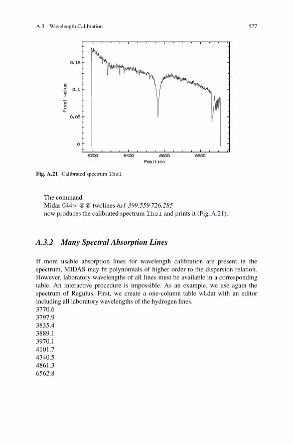
Fig. A.21 Calibrated spectrum lhs1
The commandMidas 044> @@ twolines hs1 399.559 726.285now produces the calibrated spectrum lhs1 and prints it (Fig. A.21).
A.3.2 Many Spectral Absorption Lines
If more usable absorption lines for wavelength calibration are present in thespectrum, MIDAS may fit polynomials of higher order to the dispersion relation.However, laboratory wavelengths of all lines must be available in a correspondingtable. An interactive procedure is impossible. As an example, we use again thespectrum of Regulus. First, we create a one-column table wl.dat with an editorincluding all laboratory wavelengths of the hydrogen lines.3770.63797.93835.43889.13970.14101.74340.54861.36562.8
578 A The MIDAS Data Reduction
Fig. A.22 Line identification with a line table
Midas works with its own table format in which we transform wl.dat. For asingle-column table, this is simple and we give the column of wl.dat the nameWAVE.
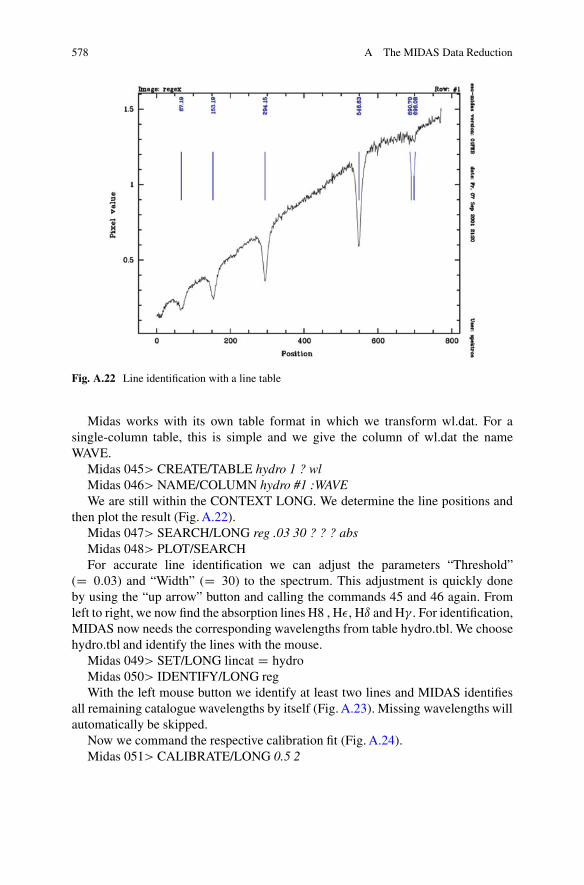
Midas 045> CREATE/TABLE hydro 1 ? wlMidas 046> NAME/COLUMN hydro #1 :WAVEWe are still within the CONTEXT LONG. We determine the line positions and
then plot the result (Fig. A.22).Midas 047> SEARCH/LONG reg .03 30 ? ? ? absMidas 048> PLOT/SEARCHFor accurate line identification we can adjust the parameters “Threshold”
(D 0:03) and “Width” (D 30) to the spectrum. This adjustment is quickly doneby using the “up arrow” button and calling the commands 45 and 46 again. Fromleft to right, we now find the absorption lines H8 , H�, Hı and H� . For identification,MIDAS now needs the corresponding wavelengths from table hydro.tbl. We choosehydro.tbl and identify the lines with the mouse.
Midas 049> SET/LONG lincat D hydroMidas 050> IDENTIFY/LONG regWith the left mouse button we identify at least two lines and MIDAS identifies
all remaining catalogue wavelengths by itself (Fig. A.23). Missing wavelengths willautomatically be skipped.
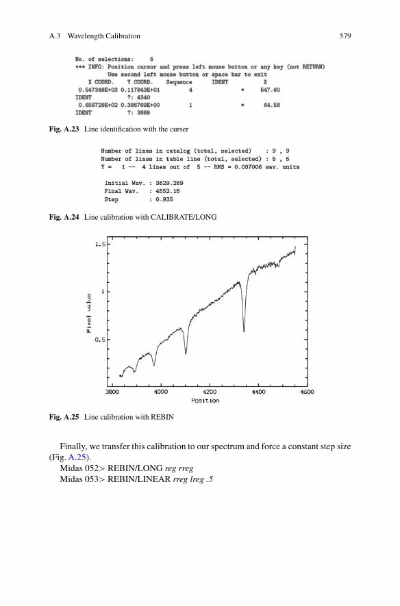
Now we command the respective calibration fit (Fig. A.24).Midas 051> CALIBRATE/LONG 0.5 2
A.3 Wavelength Calibration 579
Fig. A.23 Line identification with the curser
Fig. A.24 Line calibration with CALIBRATE/LONG
Fig. A.25 Line calibration with REBIN
Finally, we transfer this calibration to our spectrum and force a constant step size(Fig. A.25).
Midas 052> REBIN/LONG reg rregMidas 053> REBIN/LINEAR rreg lreg .5

580 A The MIDAS Data Reduction
Fig. A.26 Spectrum of Rigel in black. For comparison, a spectrum of Regulus is shown in red(Courtesy: D. Goretzki)
A.3.3 Prism Spectra
Unlike grating spectra, prism spectra have a non-negligible non-linear dispersion inthe form of a polynomial. No context for prism spectroscopy has been developedin MIDAS. However, it is quite possible to find a dispersion relation, if sufficientlymany lines as reference points are available. A spectrum of Rigel (Fig. A.26) showsthe corresponding procedure as an example. The spectrum has some hydrogen lines.One can calibrate the spectrum with CALIBRATE/LONG with the correspondingparameter settings (tolerance D 5 and polynomial degree D 2). The result is shownin black and a spectrum of Regulus for comparison is shown in red.
One can see that both calibrations differ at the spectral interval limits. The tablecompares the literature values with those from the spectrum of Rigel.
Ion Measurement LiteratureCaII 3932:9 3933
HeI 4026:2 4026
HeI 4465:2 4471
MgII 4474:0 4481
A.3 Wavelength Calibration 581
Fig. A.27 Detection of catalogue calibration lines
Fig. A.28 Line positions found with the cursor
A.3.4 The Use of a Comparison Spectrum
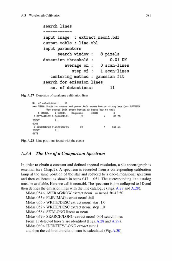
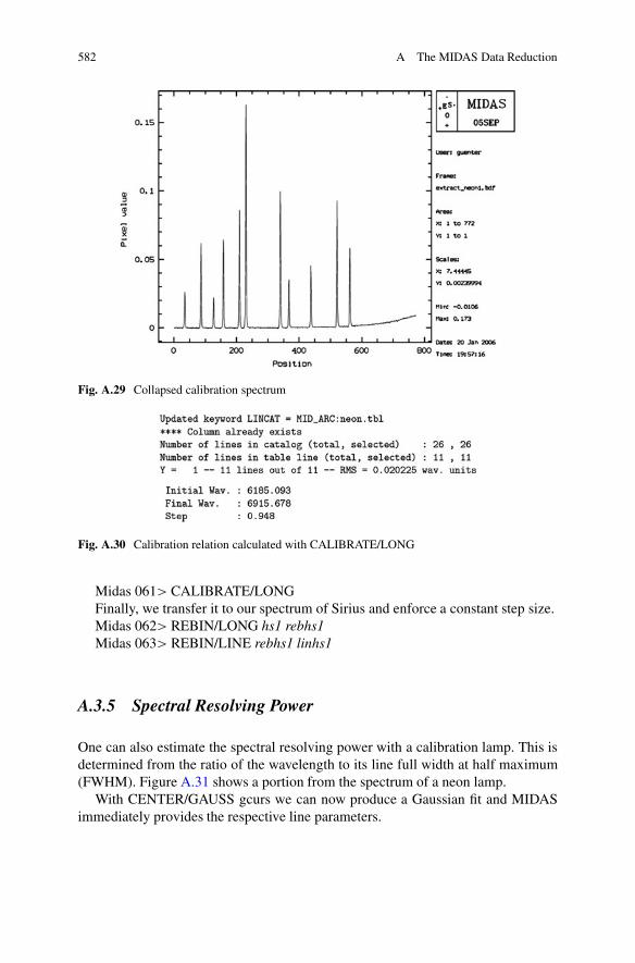
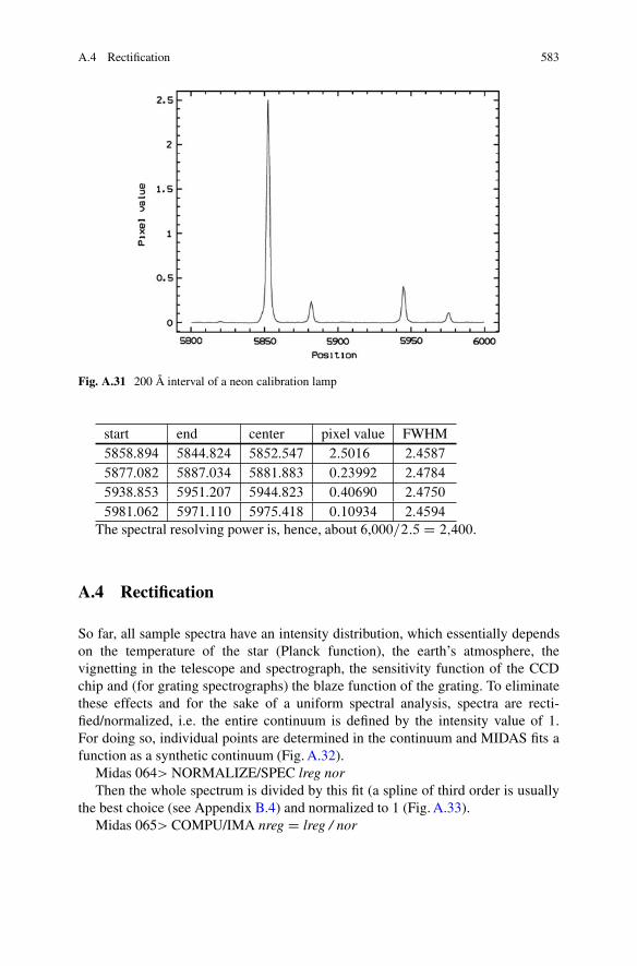
In order to obtain a constant and defined spectral resolution, a slit spectrograph isessential (see Chap. 2). A spectrum is recorded from a corresponding calibrationlamp at the same position of the star and reduced to a one-dimensional spectrumand then calibrated as shown in steps 047 � 051. The corresponding line catalogmust be available. Here we call it neon.tbl. The spectrum is first collapsed to 1D andthen defines the emission lines with the line catalogue (Figs. A.27 and A.28).
Midas 054> AVERAG/ROW extract neon1 D neon1.fts 42,50Midas 055> FLIP/IMAG extract neon1.bdfMidas 056> WRITE/DESC extract neon1 start 1.0Midas 057> WRITE/DESC extract neon1 step 1.0Midas 058> SET/LONG lincat D neonMidas 059> SEARCH/LONG extract neon1 0.01 search linesFrom 11 detected lines 2 are identified (Figs. A.28 and A.29).Midas 060> IDENTIFY/LONG extract neon1and then the calibration relation can be calculated (Fig. A.30).
582 A The MIDAS Data Reduction
Fig. A.29 Collapsed calibration spectrum
Fig. A.30 Calibration relation calculated with CALIBRATE/LONG
Midas 061> CALIBRATE/LONGFinally, we transfer it to our spectrum of Sirius and enforce a constant step size.Midas 062> REBIN/LONG hs1 rebhs1Midas 063> REBIN/LINE rebhs1 linhs1
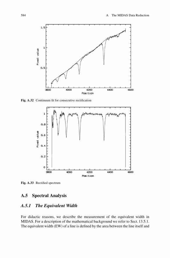
A.3.5 Spectral Resolving Power
One can also estimate the spectral resolving power with a calibration lamp. This isdetermined from the ratio of the wavelength to its line full width at half maximum(FWHM). Figure A.31 shows a portion from the spectrum of a neon lamp.
With CENTER/GAUSS gcurs we can now produce a Gaussian fit and MIDASimmediately provides the respective line parameters.
A.4 Rectification 583
Fig. A.31 200 Å interval of a neon calibration lamp
start end center pixel value FWHM5858:894 5844:824 5852:547 2:5016 2:4587
5877:082 5887:034 5881:883 0:23992 2:4784
5938:853 5951:207 5944:823 0:40690 2:4750
5981:062 5971:110 5975:418 0:10934 2:4594
The spectral resolving power is, hence, about 6,000=2:5 D 2;400.
A.4 Rectification
So far, all sample spectra have an intensity distribution, which essentially dependson the temperature of the star (Planck function), the earth’s atmosphere, thevignetting in the telescope and spectrograph, the sensitivity function of the CCDchip and (for grating spectrographs) the blaze function of the grating. To eliminatethese effects and for the sake of a uniform spectral analysis, spectra are recti-fied/normalized, i.e. the entire continuum is defined by the intensity value of 1.For doing so, individual points are determined in the continuum and MIDAS fits afunction as a synthetic continuum (Fig. A.32).
Midas 064> NORMALIZE/SPEC lreg norThen the whole spectrum is divided by this fit (a spline of third order is usually
the best choice (see Appendix B.4) and normalized to 1 (Fig. A.33).Midas 065> COMPU/IMA nreg D lreg / nor
584 A The MIDAS Data Reduction
Fig. A.32 Continuum fit for consecutive rectification
Fig. A.33 Rectified spectrum
A.5 Spectral Analysis
A.5.1 The Equivalent Width
For didactic reasons, we describe the measurement of the equivalent width inMIDAS. For a description of the mathematical background we refer to Sect. 13.5.1.The equivalent width (EW) of a line is defined by the area between the line itself and
A.5 Spectral Analysis 585
Fig. A.34 Estimation of the line equivalent width
Fig. A.35 Estimation of the line equivalent width
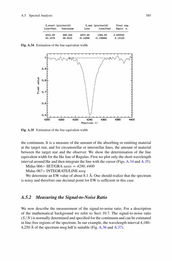
the continuum. It is a measure of the amount of the absorbing or emitting materialat the target star, and for circumstellar or interstellar lines, the amount of materialbetween the target star and the observer. We show the determination of the lineequivalent width for the H˛ line of Regulus. First we plot only the short wavelengthinterval around H˛ and then integrate the line with the cursor (Figs. A.34 and A.35).
Midas 066> SET/GRA xaxis D 4280; 4400Midas 067> INTEGRATE/LINE nregWe determine an EW value of about 8.1 Å. One should realize that the spectrum
is noisy and therefore one decimal point for EW is sufficient in this case.
A.5.2 Measuring the Signal-to-Noise Ratio
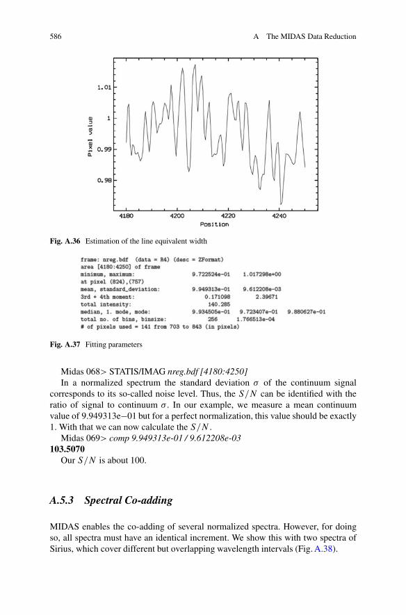
We now describe the measurement of the signal-to-noise ratio. For a descriptionof the mathematical background we refer to Sect. 10.7. The signal-to-noise ratio(S=N ) is normally determined and specified for the continuum and can be estimatedin line-free regions of the spectrum. In our example, the wavelength interval 4,180–4,250 Å of the spectrum nreg.bdf is suitable (Fig. A.36 and A.37).
586 A The MIDAS Data Reduction
Fig. A.36 Estimation of the line equivalent width
Fig. A.37 Fitting parameters
Midas 068> STATIS/IMAG nreg.bdf [4180:4250]In a normalized spectrum the standard deviation � of the continuum signal
corresponds to its so-called noise level. Thus, the S=N can be identified with theratio of signal to continuum � . In our example, we measure a mean continuumvalue of 9.949313e�01 but for a perfect normalization, this value should be exactly1. With that we can now calculate the S=N .
Midas 069> comp 9.949313e-01 / 9.612208e-03103.5070
Our S=N is about 100.
A.5.3 Spectral Co-adding
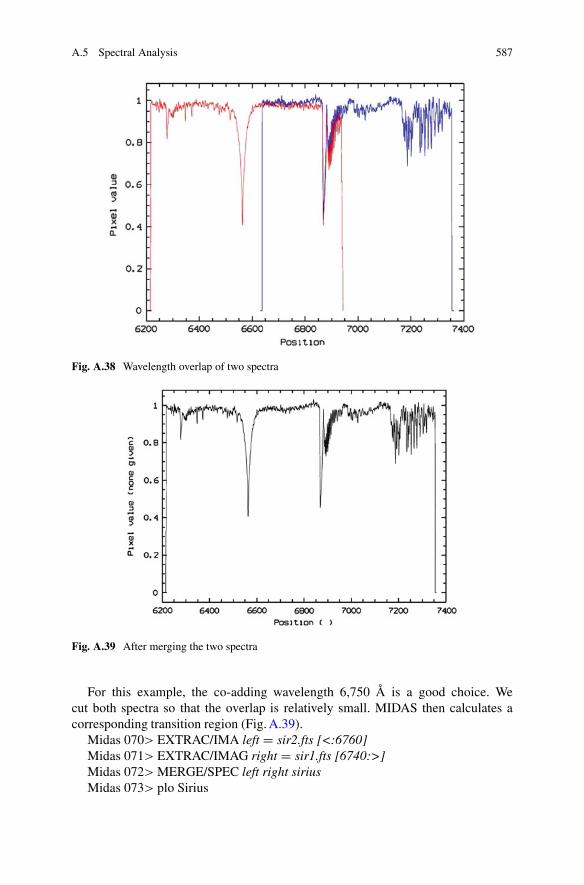
MIDAS enables the co-adding of several normalized spectra. However, for doingso, all spectra must have an identical increment. We show this with two spectra ofSirius, which cover different but overlapping wavelength intervals (Fig. A.38).
A.5 Spectral Analysis 587
Fig. A.38 Wavelength overlap of two spectra
Fig. A.39 After merging the two spectra
For this example, the co-adding wavelength 6,750 Å is a good choice. Wecut both spectra so that the overlap is relatively small. MIDAS then calculates acorresponding transition region (Fig. A.39).
Midas 070> EXTRAC/IMA left D sir2.fts [<:6760]Midas 071> EXTRAC/IMAG right D sir1.fts [6740:>]Midas 072> MERGE/SPEC left right siriusMidas 073> plo Sirius
588 A The MIDAS Data Reduction
Fig. A.40 Labeling within the MIDAS graphic window. Co-adding the two spectra
Finally, we convert the coupled spectrum into a 1-dimensional fits format.Midas 074> OUTDISK/FITS sirius.bdf sirius.fts
A.5.4 Window Texts
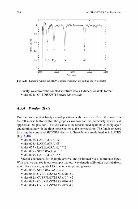
One can insert text at freely elected positions with the cursor. To do this, one usesthe left mouse button within the graphics window and the previously written textappears at that position. This text can also be repositioned again by clicking againand terminating with the right mouse button at the new position. The font is selectedby using the command SET/GRA font D ?. Greek letters are defined as in LATEX(Fig. A.40).
Midas 075> LABEL/GRA H�
Midas 076> LABEL/GRA Hı
Midas 077> LABEL/GRA H� ? ? 2Midas 078> SET/GRA font D 1Midas 079> LABEL/GRA H-8Special characters, for example arrows, are positioned via a coordinate input.
With that we can see in our example that our wavelength calibration was relativelygood. For instance, symbol 15 is an upward pointing arrow.
Midas 080> SET/GRA color D 4Midas 081> OVERPL/SYM 15 4340,.4 2Midas 082> OVERPL/SYM 15 4101,.4 2Midas 083> OVERPL/SYM 15 3970,.4 2Midas 084> OVERPL/SYM 15 3889,.4 2
A.5 Spectral Analysis 589
Once texts and labels are set, one cannot move or change them again. It makessense to keep the corresponding commands in a script.
A.5.5 Exporting Reduced Spectra: Fits/ASCII/Postscript
The export to a fits format has already been briefly described above.Midas 085> OUTDISK/FITS sirius.bdf sirius.ftsHowever, the notes in the graphics window are not exported. The export as ASCII
file can be performed in any operating system. The 1-dimensional spectrum is thenfirst converted into a table format and then printed as ASCII. But first one needs totell MIDAS the file name. As an example, we export the normalized spectrum ofRigel.
Midas 086> COPY/IT nrig nrig wavelengthMidas 087> ASSIGN/PRINT file nrig.datMidas 088> PRINT/TABL nrig NMidas 089> $ls nrig.dat1 3.79489eC03 9.47901e-01
2 3.79539eC03 9.33670e-013 3.79589eC03 9.18116e-014 3.79639eC03 8.77109e-015 3.79689eC03 8.34155e-016 3.79739eC03 7.89637e-017 3.79789eC03 7.54711e-018 3.79839eC03 7.42803e-01
: : :
Notes and other texts are not exported.
A.5.6 Postscript
Images and graphics in PostScript format are very popular in science and areespecially used in the LATEX environment. Export into this format is very simplein MIDAS .
Midas 090> COPY/GRA postscriptNote, the command must be carried out literally. The resulting file can then be
renamed and printed.
590 A The MIDAS Data Reduction
Fig. A.41 Output for postscript format
A.5.7 Printing
MIDAS must know the printer for printing graphic content.The file /midas/01FEBpl1.1/systab/ascii/plot/agldevs.dat contains an instrument
list of all the peripherals that can be addressed by MIDAS. At the end of this list theROOT can add an appropriate printer. The printer name must also be listed in the/etc/printcap directory. Now we can send the image to the printer (Fig. A.41).
Midas 091> COPY/GRA eps360The picture fills exactly one A4 page, even if the graphics window has a different
format.Midas 092> BYEuser@linux:� >
Appendix BImportant Functions and Equations
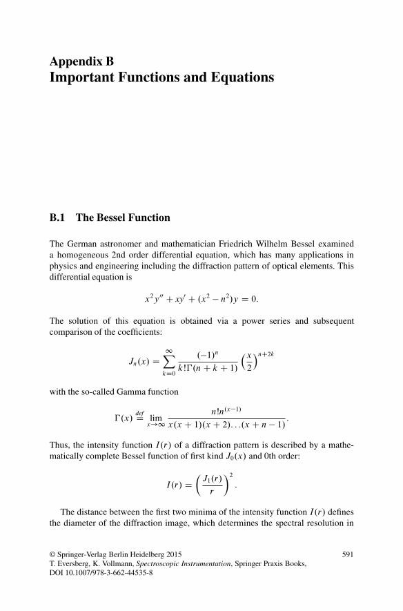
B.1 The Bessel Function
The German astronomer and mathematician Friedrich Wilhelm Bessel examineda homogeneous 2nd order differential equation, which has many applications inphysics and engineering including the diffraction pattern of optical elements. Thisdifferential equation is
x2y00 C xy0 C .x2 � n2/y D 0:
The solution of this equation is obtained via a power series and subsequentcomparison of the coefficients:
Jn.x/ D1X
kD0
.�1/n
kŠ�.n C k C 1/
�x
2
�nC2k
with the so-called Gamma function
�.x/defD lim
x!1nŠn.x�1/
x.x C 1/.x C 2/: : :.x C n � 1/:
Thus, the intensity function I.r/ of a diffraction pattern is described by a mathe-matically complete Bessel function of first kind J0.x/ and 0th order:
I.r/ D�
J1.r/
r
�2
:
The distance between the first two minima of the intensity function I.r/ definesthe diameter of the diffraction image, which determines the spectral resolution in
© Springer-Verlag Berlin Heidelberg 2015T. Eversberg, K. Vollmann, Spectroscopic Instrumentation, Springer Praxis Books,DOI 10.1007/978-3-662-44535-8
591
592 B Important Functions and Equations
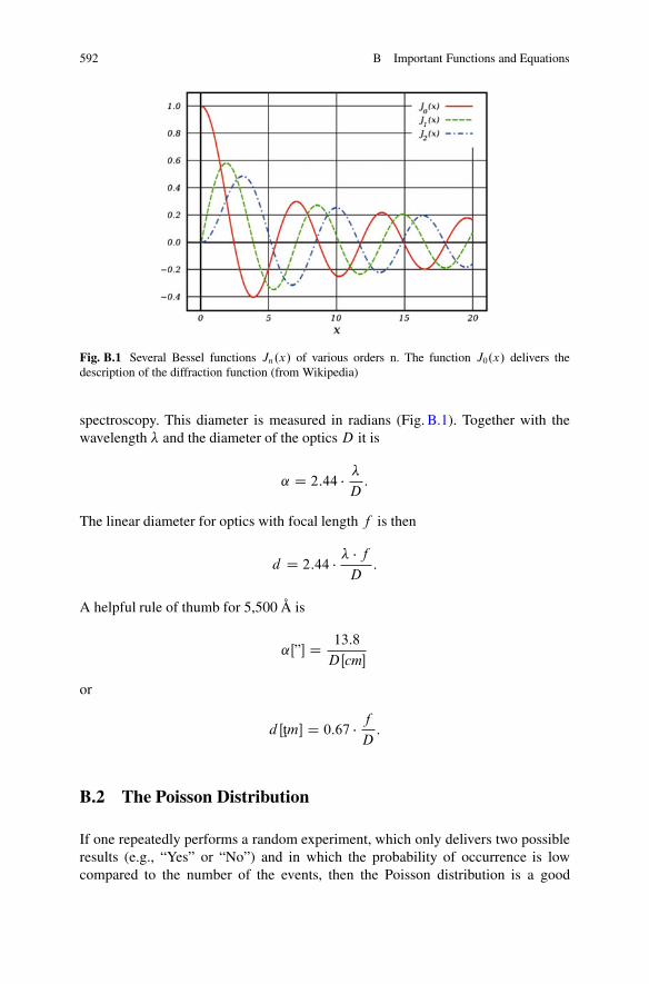
Fig. B.1 Several Bessel functions Jn.x/ of various orders n. The function J0.x/ delivers thedescription of the diffraction function (from Wikipedia)
spectroscopy. This diameter is measured in radians (Fig. B.1). Together with thewavelength � and the diameter of the optics D it is
˛ D 2:44 � �
D:
The linear diameter for optics with focal length f is then
d D 2:44 � � � f
D:
A helpful rule of thumb for 5,500 Å is
˛Œ”� D 13:8
DŒcm�
or
dŒtm� D 0:67 � f
D:
B.2 The Poisson Distribution
If one repeatedly performs a random experiment, which only delivers two possibleresults (e.g., “Yes” or “No”) and in which the probability of occurrence is lowcompared to the number of the events, then the Poisson distribution is a good
B.2 The Poisson Distribution 593
approximation for the corresponding probability distribution. For example, ifphotons reach a detector, this is a purely random event. To make quantitativestatements about this process, one needs to count these events within a given timeunder constant conditions. The variations show a specific distribution function (inthis case, the Poisson distribution). This indicates how likely it is to count n photonsin time t , if the expectance value is k. This is
P.n; t; k/ D kn
nŠe�k:
By adding up all n particles, the corresponding probability must be 1, of course.With the definition of the exponential function ex D P
nxn
nŠwe obtain
Xn
P.n; t; k/ D e�kX
n
kn
nŠD e�k � ek D 1
and with the definition of the mean value < n > we obtain
< n >DX
n
nP.n; t; k/ D e�kX
n
n � kn
nŠD k � e�k
Xn
:kn�1
.n � 1/ŠD k:
The expectance value k is therefore equal to the average of n. For each distribution,including the Poisson distribution, the variance �2 is given by �2 D ˝
n2˛ � hni2. For
the Poisson distribution we have
˝n2
˛ DX
n
n2P.n/ D e�kX
n
n � .n � 1/ C 1
nŠ� kn
D e�k
"Xn
k2 kn�2
.n � 2/ŠC
Xn
kkn�1
.n � 1/Š
#D k2 C k:
For hni2, the result is �2 D k ) � D pk. The Poisson distribution thus depends
only on the expectance value. The Poisson distribution is generally valid even fornon-integer n. For this case, we define n � x and we obtain
P.x; k/ D kx
�.x C 1/e�k
by using the Gamma function from Appendix B.1 which is �.x C 1/ D nŠ forinteger numbers x D n. It should be noted that the sum changes to an integral if wechange from discrete (integer) n to continuous (any) x:
hni2 D1X
nD0
nP.n/ ! hxi2 DZ 1
nD0
xP.x/dx D k:
594 B Important Functions and Equations
0.8
K1 = 0.3
67%
K2 = 3K3 = 5
0.6
P(x
)
0.4
0.2
00 2 4
x
6 8 10
K - σ K + σ K + 2σ K + 3σK
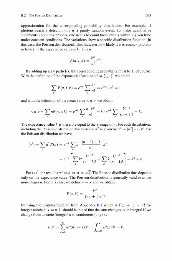
Fig. B.2 Several Poisson distributions P.x/ with different values of k ( 0.3 , 3 and 5), anddepiction of the probability for the interval [k2 � �; k2 C � ]
In Fig. B.2 three typical Poisson distributions are shown. For k � 1 the Poissondistribution is strongly asymmetric and the argument x for the maximum value Pmax
of the distribution is always smaller than k. For curve 1 in Fig. B.2 we have xmax D 0
and k D 0:3. For large k, the Poisson distribution becomes a Gaussian distributionwith � D p
k (curve 3):
lim PPoiss D 1p2k
e�.n�k/2=2k:
The probability of finding a value x within the standard deviation � D pk of the
average value k can be calculated via W.k; �/ D R kC�
k��P.x; k/dx. We obtain (see
Fig. B.2):
k ˙ � ) W.k; �/ D 0:67
k ˙ 2� ) W.k; �/ D 0:95
k ˙ 3� ) W.k; �/ D 0:997
However, in spectroscopy we measure photons, discrete particles, and instead ofcontinuous values for x we have to change to discrete values of n. The Poissondistribution for discrete n is called the binomial distribution.
B.3 The Fresnel Equations
When light passes a boundary layer between two media, one part of the lightbeam is reflected and the other transmitted. A quantitative calculation succeeded
B.3 The Fresnel Equations 595
that of Jean Fresnel for isotropic and non-ferromagnetic materials. Considering anelectromagnetic wave, the ratio between the electric and magnetic field strength is
H D n �r
�0
0
� E:
The constants �0 or 0 are the fundamental dielectric and magnetic constants andn is the refractive index of the irradiated material. At normal incidence1 we have
E 0 D n � n00
n C n00 � E and E 00 D 2n
n C n00 � E:
The reflected light is indicated by a straight line whereas the diffracted lightis indicated by two lines. For reflection, the wave intensity is the square of theamplitude:
�E 0
E
�2
D�
n � n00
n C n00
�2
D R:
The reflectivity R is thus the ratio of reflected to incident wave intensity and thetransmissivity T is the ratio of transmitted to incident wave intensity. Because of theconservation of energy we have R C T D 1 and thus
T D 1 � R D 4nn00
.n C n00/2:
The oblique wave incidence can be represented by the individual components,which oscillate perpendicularly and parallel to the plane of incidence (1 for verticaland 2 for parallel).
R1 D sin2.ˇ00 � ˇ/
sin2.ˇ00 C ˇ/
R2 D tan2.ˇ00 � ˇ/
tan2.ˇ00 C ˇ/
T1 D sin 2ˇ � sin 2ˇ00
sin2.ˇ00 C ˇ/
T2 D sin 2ˇ � sin 2ˇ00
sin2.ˇ00 C ˇ/ � cos2.ˇ00 � ˇ/
with the angles of incident, reflection and dispersion ˇ, ˇ0 and ˇ00.
1The Fresnel equations also include dielectric materials, magnetic permeability and polarisation.For a detailed general discussion we refer to the corresponding literature.
596 B Important Functions and Equations
B.4 The Spline Function
To normalize the spectrum of a continuum to 1, a continuous function has to befitted to the continuum of the original spectrum and then divided into the originalspectrum. For the fit we use reference points between the spectral lines which, apartfrom the noise, are well defined in intensity. Here we encounter a difficulty. Inthe wavelength intervals of emission or absorption lines there are no continuumreference points available. Nevertheless, to find an appropriate continuum functionwithin the lines, we need a continuous function that has sufficient stability within thespectral lines and which reliably approximates the real continuum. Such a functionis a spline2
To find a function that passes exactly through a predetermined number of pointsone has to interpolate. For interpolation of n intervals with nC1 nodes one needs tofind a function of order n, which passes exactly through all the specified points.However, classical polynomials tend to oscillate between the supporting points(e.g., atomic lines). To avoid oscillations one uses continuous splines of 3rd order(cubic splines), which are partially composed of individual polynomials and havethe lowest possible curvature. It is also required that the curve be continuous upto the second derivative at all junctions. For each interpolation interval betweentwo nodes, four coefficients of the cubic function must be found. For n C 1 nodesthere are 4n necessary coefficients. To determine the function coefficients, we usethe requirement of identical function values at the n junctions and thus obtain2n interpolation conditions. In addition at all connection points, continuity of thefunction as well as its first and second derivative must be ensured. Hence, we getanother 2.n � 1/ interpolation conditions. Thus, we have 2n C 2n � 2 D 4n � 2
interpolation conditions. To determine the 4n coefficients two conditions are stillmissing. We get them from the requirement that the function derivatives (slopes)should not change at the two function ends. Thus, the second derivative of thefunction is zero there.
We start with n C 1 different x nodes .xi ; yi / sorted in ascending order, withi D 1; : : :; n, for which we seek the spline f .x/ (respectively I.�/ in the definitionof the spectral continuum). For each section i we define the third-order polynomialsi .x/:
si .x/ D ai .x � xi /3 C bi.x � xi /
2 C ci .x � xi / C di :
With the different interval lengths hi D xiC1 � xi we get for the interval i thefollowing conditions for si and its first and second derivatives of s0
i and s00i :
si .xi / D di D yi (B.1)
2The term comes from the constriction of ships, where one determined the shape of the plankingusing a flexible ruler, called spline, for minimum mechanical stress.
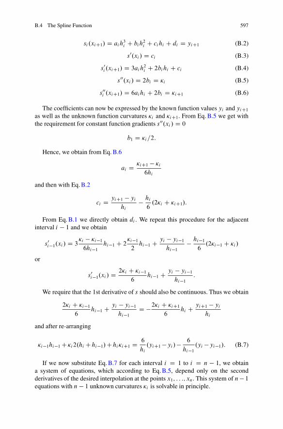
B.4 The Spline Function 597
si .xiC1/ D ai h3i C bih
2i C ci hi C di D yiC1 (B.2)
s0.xi / D ci (B.3)
s0i .xiC1/ D 3ai h
2i C 2bi hi C ci (B.4)
s00.xi / D 2bi D �i (B.5)
s00i .xiC1/ D 6aihi C 2bi D �iC1 (B.6)
The coefficients can now be expressed by the known function values yi and yiC1
as well as the unknown function curvatures �i and �iC1. From Eq. B.5 we get withthe requirement for constant function gradients s00.xi / D 0
b1 D �i =2:
Hence, we obtain from Eq. B.6
ai D �iC1 � �i
6hi
and then with Eq. B.2
ci D yiC1 � yi
hi
� hi
6.2�i C �iC1/:
From Eq. B.1 we directly obtain di . We repeat this procedure for the adjacentinterval i � 1 and we obtain
s0i�1.xi / D 3
�i � �i�1
6hi�1
hi�1 C 2�i�1
2hi�1 C yi � yi�1
hi�1
� hi�1
6.2�i�1 C �i /
or
s0i�1.xi / D 2�i C �i�1
6hi�1 C yi � yi�1
hi�1
:
We require that the 1st derivative of s should also be continuous. Thus we obtain
2�i C �i�1
6hi�1 C yi � yi�1
hi�1
D �2�i C �iC1
6hi C yiC1 � yi
hi
and after re-arranging
�i�1hi�1 C�i 2.hi Chi�1/ Chi �iC1 D 6
hi
.yiC1 � yi / � 6
hi�1
.yi � yi�1/: (B.7)
If we now substitute Eq. B.7 for each interval i D 1 to i D n � 1, we obtaina system of equations, which according to Eq. B.5, depend only on the secondderivatives of the desired interpolation at the points x1; : : :; xn. This system of n � 1
equations with n � 1 unknown curvatures �i is solvable in principle.
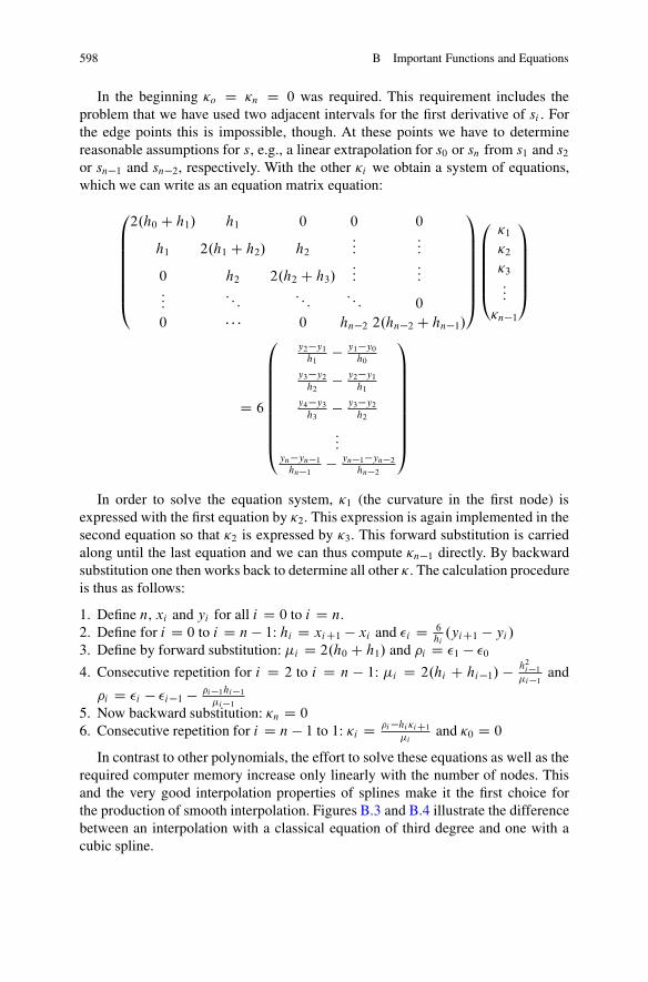
598 B Important Functions and Equations
In the beginning �o D �n D 0 was required. This requirement includes theproblem that we have used two adjacent intervals for the first derivative of si . Forthe edge points this is impossible, though. At these points we have to determinereasonable assumptions for s, e.g., a linear extrapolation for s0 or sn from s1 and s2
or sn�1 and sn�2, respectively. With the other �i we obtain a system of equations,which we can write as an equation matrix equation:
0BBBBBBB@
2.h0 C h1/ h1 0 0 0
h1 2.h1 C h2/ h2
::::::
0 h2 2.h2 C h3/:::
::::::
: : :: : :
: : : 0
0 � � � 0 hn�2 2.hn�2 C hn�1/
1CCCCCCCA
0BBBBB@
�1
�2
�3
:::
�n�1
1CCCCCA
D 6
0BBBBBBBBB@
y2�y1
h1� y1�y0
h0
y3�y2
h2� y2�y1
h1
y4�y3
h3� y3�y2
h2
:::yn�yn�1
hn�1� yn�1�yn�2
hn�2
1CCCCCCCCCA
In order to solve the equation system, �1 (the curvature in the first node) isexpressed with the first equation by �2. This expression is again implemented in thesecond equation so that �2 is expressed by �3. This forward substitution is carriedalong until the last equation and we can thus compute �n�1 directly. By backwardsubstitution one then works back to determine all other �. The calculation procedureis thus as follows:
1. Define n, xi and yi for all i D 0 to i D n.2. Define for i D 0 to i D n � 1: hi D xiC1 � xi and �i D 6
hi.yiC1 � yi /
3. Define by forward substitution: i D 2.h0 C h1/ and �i D �1 � �0
4. Consecutive repetition for i D 2 to i D n � 1: i D 2.hi C hi�1/ � h2i�1
i�1and
�i D �i � �i�1 � �i�1hi�1
i�1
5. Now backward substitution: �n D 0
6. Consecutive repetition for i D n � 1 to 1: �i D �i �hi �iC1
iand �0 D 0
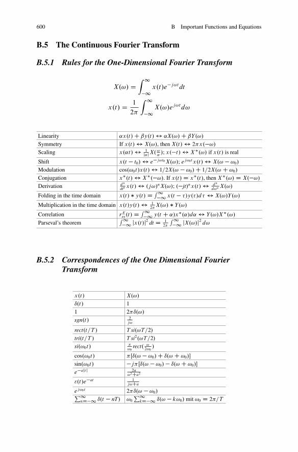
In contrast to other polynomials, the effort to solve these equations as well as therequired computer memory increase only linearly with the number of nodes. Thisand the very good interpolation properties of splines make it the first choice forthe production of smooth interpolation. Figures B.3 and B.4 illustrate the differencebetween an interpolation with a classical equation of third degree and one with acubic spline.
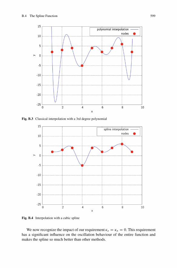
B.4 The Spline Function 599
Fig. B.3 Classical interpolation with a 3rd degree polynomial
Fig. B.4 Interpolation with a cubic spline
We now recognize the impact of our requirement �o D �n D 0. This requirementhas a significant influence on the oscillation behaviour of the entire function andmakes the spline so much better than other methods.
600 B Important Functions and Equations
B.5 The Continuous Fourier Transform
B.5.1 Rules for the One-Dimensional Fourier Transform
X.!/ DZ 1
�1x.t/e�j!t dt
x.t/ D 1
2
Z 1
�1X.!/ej!td!
Linearity ˛x.t/ C ˇy.t/ $ ˛X.!/ C ˇY.!/
Symmetry If x.t/ $ X.!/, then X.t/ $ 2x.�!/
Scaling x.˛t/ $ 1j˛j
X. !˛
/; x.�t / $ X�.!/ if x.t/ is real
Shift x.t � t0/ $ e�j!t0 X.!/; ej!0t x.t/ $ X.! � !0/
Modulation cos.!0t/x.t/ $ 1=2X.! � !0/ C 1=2X.! C !0/
Conjugation x�.t / $ X�.�!/. If x.t/ D x�.t /, then X�.!/ D X.�!/
Derivation dn
dtn x.t/ $ .j!/nX.!/; .�jt/nx.t/ $ dn
d!n X.!/
Folding in the time domain x.t/ � y.t/ D R1
�1
x.t � /y. /d $ X.!/Y.!/
Multiplication in the time domain x.t/y.t/ $ 12
X.!/ � Y.!/
Correlation rExy.t / D R
1
�1
y.t C ˛/x�.˛/d˛ $ Y.!/X�.!/
Parseval’s theoremR
1
�1
jx.t/j2 dt D 12
R1
�1
jX.!/j2d!
B.5.2 Correspondences of the One Dimensional FourierTransform
x.t/ X.!/
ı.t/ 1
1 2ı.!/
sgn.t / 2j!
rect.t=T / T si.!T=2/
tri.t=T / T si2.!T=2/
si.!0t/ !0
rect. !2!0
/
cos.!0t/ Œı.! � !0/ C ı.! C !0/�
sin.!0t/ �jŒı.! � !0/ � ı.! C !0/�
e�ajtj 2a!2
Ca2
".t/e�at 1j!Ca
ej!0t 2ı.! � !0/P1
nD�1
ı.t � nT/ !0
P1
kD�1
ı.! � k!0/ mit !0 D 2=T
Appendix CDiffraction Indices of Various Glasses
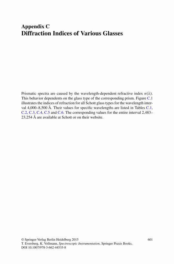
Prismatic spectra are caused by the wavelength-dependent refractive index n.�/.This behavior dependents on the glass type of the corresponding prism. Figure C.1illustrates the indices of refraction for all Schott glass types for the wavelength inter-val 4,000–8,500 Å. Their values for specific wavelengths are listed in Tables C.1,C.2, C.3, C.4, C.5 and C.6. The corresponding values for the entire interval 2,483–23,254 Å are available at Schott or on their website.
© Springer-Verlag Berlin Heidelberg 2015T. Eversberg, K. Vollmann, Spectroscopic Instrumentation, Springer Praxis Books,DOI 10.1007/978-3-662-44535-8
601
602 C Diffraction Indices of Various Glasses
Fig. C.1 Graph of therefraction indices of allavailable Schott glass typesfor the wavelength interval4,000–8,500 Å (Schott). Forvisual wavelengths theindices of refraction arebetween 1.4 and 2. Theyincrease towards shorterwavelengths for all glasses
C Diffraction Indices of Various Glasses 603
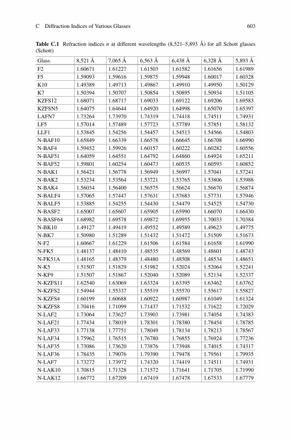
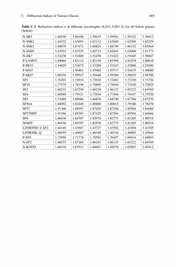
Table C.1 Refraction indices n at different wavelengths (8,521–5,893 Å) for all Schott glasses(Schott)
Glass 8,521 Å 7,065 Å 6,563 Å 6,438 Å 6,328 Å 5,893 Å
F2 1.60671 1.61227 1.61503 1.61582 1.61656 1.61989
F5 1.59093 1.59616 1.59875 1.59948 1.60017 1.60328
K10 1.49389 1.49713 1.49867 1.49910 1.49950 1.50129
K7 1.50394 1.50707 1.50854 1.50895 1.50934 1.51105
KZFS12 1.68071 1.68717 1.69033 1.69122 1.69206 1.69583
KZFSN5 1.64075 1.64644 1.64920 1.64998 1.65070 1.65397
LAFN7 1.73264 1.73970 1.74319 1.74418 1.74511 1.74931
LF5 1.57014 1.57489 1.57723 1.57789 1.57851 1.58132
LLF1 1.53845 1.54256 1.54457 1.54513 1.54566 1.54803
N-BAF10 1.65849 1.66339 1.66578 1.66645 1.66708 1.66990
N-BAF4 1.59452 1.59926 1.60157 1.60222 1.60282 1.60556
N-BAF51 1.64059 1.64551 1.64792 1.64860 1.64924 1.65211
N-BAF52 1.59801 1.60254 1.60473 1.60535 1.60593 1.60852
N-BAK1 1.56421 1.56778 1.56949 1.56997 1.57041 1.57241
N-BAK2 1.53234 1.53564 1.53721 1.53765 1.53806 1.53988
N-BAK4 1.56034 1.56400 1.56575 1.56624 1.56670 1.56874
N-BALF4 1.57065 1.57447 1.57631 1.57683 1.57731 1.57946
N-BALF5 1.53885 1.54255 1.54430 1.54479 1.54525 1.54730
N-BASF2 1.65007 1.65607 1.65905 1.65990 1.66070 1.66430
N-BASF64 1.68982 1.69578 1.69872 1.69955 1.70033 1.70384
N-BK10 1.49127 1.49419 1.49552 1.49589 1.49623 1.49775
N-BK7 1.50980 1.51289 1.51432 1.51472 1.51509 1.51673
N-F2 1.60667 1.61229 1.61506 1.61584 1.61658 1.61990
N-FK5 1.48137 1.48410 1.48535 1.48569 1.48601 1.48743
N-FK51A 1.48165 1.48379 1.48480 1.48508 1.48534 1.48651
N-K5 1.51507 1.51829 1.51982 1.52024 1.52064 1.52241
N-KF9 1.51507 1.51867 1.52040 1.52089 1.52134 1.52337
N-KZFS11 1.62540 1.63069 1.63324 1.63395 1.63462 1.63762
N-KZFS2 1.54944 1.55337 1.55519 1.55570 1.55617 1.55827
N-KZFS4 1.60199 1.60688 1.60922 1.60987 1.61049 1.61324
N-KZFS8 1.70416 1.71099 1.71437 1.71532 1.71622 1.72029
N-LAF2 1.73064 1.73627 1.73903 1.73981 1.74054 1.74383
N-LAF21 1.77434 1.78019 1.78301 1.78380 1.78454 1.78785
N-LAF33 1.77138 1.77751 1.78049 1.78134 1.78213 1.78567
N-LAF34 1.75962 1.76515 1.76780 1.76855 1.76924 1.77236
N-LAF35 1.73086 1.73620 1.73876 1.73948 1.74015 1.74317
N-LAF36 1.78435 1.79076 1.79390 1.79478 1.79561 1.79935
N-LAF7 1.73272 1.73972 1.74320 1.74419 1.74511 1.74931
N-LAK10 1.70815 1.71328 1.71572 1.71641 1.71705 1.71990
N-LAK12 1.66772 1.67209 1.67419 1.67478 1.67533 1.67779
604 C Diffraction Indices of Various Glasses
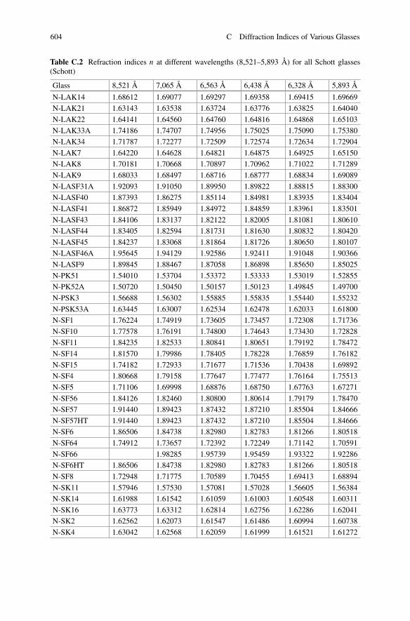
Table C.2 Refraction indices n at different wavelengths (8,521–5,893 Å) for all Schott glasses(Schott)
Glass 8,521 Å 7,065 Å 6,563 Å 6,438 Å 6,328 Å 5,893 Å
N-LAK14 1.68612 1.69077 1.69297 1.69358 1.69415 1.69669
N-LAK21 1.63143 1.63538 1.63724 1.63776 1.63825 1.64040
N-LAK22 1.64141 1.64560 1.64760 1.64816 1.64868 1.65103
N-LAK33A 1.74186 1.74707 1.74956 1.75025 1.75090 1.75380
N-LAK34 1.71787 1.72277 1.72509 1.72574 1.72634 1.72904
N-LAK7 1.64220 1.64628 1.64821 1.64875 1.64925 1.65150
N-LAK8 1.70181 1.70668 1.70897 1.70962 1.71022 1.71289
N-LAK9 1.68033 1.68497 1.68716 1.68777 1.68834 1.69089
N-LASF31A 1.92093 1.91050 1.89950 1.89822 1.88815 1.88300
N-LASF40 1.87393 1.86275 1.85114 1.84981 1.83935 1.83404
N-LASF41 1.86872 1.85949 1.84972 1.84859 1.83961 1.83501
N-LASF43 1.84106 1.83137 1.82122 1.82005 1.81081 1.80610
N-LASF44 1.83405 1.82594 1.81731 1.81630 1.80832 1.80420
N-LASF45 1.84237 1.83068 1.81864 1.81726 1.80650 1.80107
N-LASF46A 1.95645 1.94129 1.92586 1.92411 1.91048 1.90366
N-LASF9 1.89845 1.88467 1.87058 1.86898 1.85650 1.85025
N-PK51 1.54010 1.53704 1.53372 1.53333 1.53019 1.52855
N-PK52A 1.50720 1.50450 1.50157 1.50123 1.49845 1.49700
N-PSK3 1.56688 1.56302 1.55885 1.55835 1.55440 1.55232
N-PSK53A 1.63445 1.63007 1.62534 1.62478 1.62033 1.61800
N-SF1 1.76224 1.74919 1.73605 1.73457 1.72308 1.71736
N-SF10 1.77578 1.76191 1.74800 1.74643 1.73430 1.72828
N-SF11 1.84235 1.82533 1.80841 1.80651 1.79192 1.78472
N-SF14 1.81570 1.79986 1.78405 1.78228 1.76859 1.76182
N-SF15 1.74182 1.72933 1.71677 1.71536 1.70438 1.69892
N-SF4 1.80668 1.79158 1.77647 1.77477 1.76164 1.75513
N-SF5 1.71106 1.69998 1.68876 1.68750 1.67763 1.67271
N-SF56 1.84126 1.82460 1.80800 1.80614 1.79179 1.78470
N-SF57 1.91440 1.89423 1.87432 1.87210 1.85504 1.84666
N-SF57HT 1.91440 1.89423 1.87432 1.87210 1.85504 1.84666
N-SF6 1.86506 1.84738 1.82980 1.82783 1.81266 1.80518
N-SF64 1.74912 1.73657 1.72392 1.72249 1.71142 1.70591
N-SF66 1.98285 1.95739 1.95459 1.93322 1.92286
N-SF6HT 1.86506 1.84738 1.82980 1.82783 1.81266 1.80518
N-SF8 1.72948 1.71775 1.70589 1.70455 1.69413 1.68894
N-SK11 1.57946 1.57530 1.57081 1.57028 1.56605 1.56384
N-SK14 1.61988 1.61542 1.61059 1.61003 1.60548 1.60311
N-SK16 1.63773 1.63312 1.62814 1.62756 1.62286 1.62041
N-SK2 1.62562 1.62073 1.61547 1.61486 1.60994 1.60738
N-SK4 1.63042 1.62568 1.62059 1.61999 1.61521 1.61272
C Diffraction Indices of Various Glasses 605
Table C.3 Refraction indices n at different wavelengths (8,521–5,893 Å) for all Schott glasses(Schott)
N-SK5 1.60530 1.60100 1.59635 1.59581 1.59142 1.58913
N-SSK2 1.64232 1.63691 1.63112 1.63045 1.62508 1.62229
N-SSK5 1.68079 1.67471 1.66824 1.66749 1.66152 1.65844
N-SSK8 1.63923 1.63335 1.62713 1.62641 1.62068 1.61773
N-ZK7 1.52238 1.51869 1.51470 1.51423 1.51045 1.50847
P-LASF47 1.84064 1.83112 1.82110 1.81994 1.81078 1.80610
P-PK53 1.54029 1.53673 1.53288 1.53243 1.52880 1.52690
P-SF67 1.96401 1.93985 1.93717 1.91675 1.90680
P-SK57 1.60359 1.59917 1.59440 1.59384 1.58935 1.58700
SF1 1.76201 1.74916 1.73610 1.73462 1.72310 1.71736
SF10 1.77579 1.76198 1.74805 1.74648 1.73430 1.72825
SF2 1.68233 1.67249 1.66238 1.66123 1.65222 1.64769
SF4 1.80589 1.79121 1.77636 1.77468 1.76167 1.75520
SF5 1.71069 1.69986 1.68876 1.68750 1.67764 1.67270
SF56A 1.84092 1.82449 1.80800 1.80615 1.79180 1.78470
SF57 1.91366 1.89393 1.87425 1.87204 1.85504 1.84666
SF57HHT 1.91366 1.89393 1.87425 1.87204 1.85504 1.84666
SF6 1.86436 1.84707 1.82970 1.82775 1.81265 1.80518
SF6HT 1.86436 1.84707 1.82970 1.82775 1.81265 1.80518
LITHOTEC-CAF2 1.44149 1.43947 1.43727 1.43702 1.43494 1.43385
LITHOSIL-Q 1.46959 1.46667 1.46348 1.46310 1.46005 1.45844
P-SF8 1.72950 1.71778 1.70591 1.70457 1.69414 1.68893
N-SF2 1.68273 1.67265 1.66241 1.66125 1.65222 1.64769
N-KZFS5 1.68318 1.67511 1.66667 1.66570 1.65803 1.65412
606 C Diffraction Indices of Various Glasses
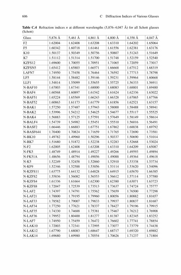
Table C.4 Refraction indices n at different wavelengths (5,876–4,047 Å) for all Schott glasses(Schott)
Glass 5,876 Å 5,461 Å 4,861 Å 4,800 Å 4,358 Å 4,047 Å
F2 1.62004 1.62408 1.63208 1.63310 1.64202 1.65064
F5 1.60342 1.60718 1.61461 1.61556 1.62381 1.63176
K10 1.50137 1.50349 1.50756 1.50807 1.51243 1.51649
K7 1.51112 1.51314 1.51700 1.51748 1.52159 1.52540
KZFS12 1.69600 1.70055 1.70951 1.71065 1.72059 1.73017
KZFSN5 1.65412 1.65803 1.66571 1.66668 1.67512 1.68319
LAFN7 1.74950 1.75458 1.76464 1.76592 1.77713 1.78798
LF5 1.58144 1.58482 1.59146 1.59231 1.59964 1.60668
LLF1 1.54814 1.55099 1.55655 1.55725 1.56333 1.56911
N-BAF10 1.67003 1.67341 1.68000 1.68083 1.68801 1.69480
N-BAF4 1.60568 1.60897 1.61542 1.61624 1.62336 1.63022
N-BAF51 1.65224 1.65569 1.66243 1.66328 1.67065 1.67766
N-BAF52 1.60863 1.61173 1.61779 1.61856 1.62521 1.63157
N-BAK1 1.57250 1.57487 1.57943 1.58000 1.58488 1.58941
N-BAK2 1.53996 1.54212 1.54625 1.54677 1.55117 1.55525
N-BAK4 1.56883 1.57125 1.57591 1.57649 1.58149 1.58614
N-BALF4 1.54739 1.54982 1.55451 1.55510 1.56016 1.56491
N-BASF2 1.66446 1.66883 1.67751 1.67862 1.68838 1.69792
N-BASF644 1.70400 1.70824 1.71659 1.71765 1.72690 1.73581
N-BK10 1.49782 1.49960 1.50296 1.50337 1.50690 1.51014
N-BK7 1.51680 1.51872 1.52238 1.52283 1.52668 1.53024
N-F2 1.62005 1.62408 1.63208 1.63310 1.64209 1.65087
N-FK5 1.48749 1.48914 1.49227 1.49266 1.49593 1.49894
N-FK51A 1.48656 1.48794 1.49056 1.49088 1.49364 1.49618
N-K5 1.52249 1.52458 1.52860 1.52910 1.53338 1.53734
N-KF9 1.52346 1.52588 1.53056 1.53114 1.53620 1.54096
N-KZFS11 1.63775 1.64132 1.64828 1.64915 1.65670 1.66385
N-KZFS2 1.55836 1.56082 1.56553 1.56612 1.57114 1.57580
N-KZFS4 1.61336 1.61664 1.62300 1.62380 1.63071 1.63723
N-KZFS8 1.72047 1.72539 1.73513 1.73637 1.74724 1.75777
N-LAF2 1.74397 1.74791 1.75562 1.75659 1.76500 1.77298
N-LAF21 1.78800 1.79195 1.79960 1.80056 1.80882 1.81657
N-LAF33 1.78582 1.79007 1.79833 1.79937 1.80837 1.81687
N-LAF34 1.77250 1.77621 1.78337 1.78427 1.79196 1.79915
N-LAF35 1.74330 1.74688 1.75381 1.75467 1.76212 1.76908
N-LAF36 1.79952 1.80400 1.81277 1.81387 1.82345 1.83252
N-LAF7 1.74950 1.75459 1.76472 1.76602 1.77741 1.78854
N-LAK10 1.72003 1.72341 1.72995 1.73077 1.73779 1.74438
N-LAK12 1.67790 1.68083 1.68647 1.68717 1.69320 1.69882
N-LAK14 1.69680 1.69980 1.70554 1.70626 1.71237 1.71804
C Diffraction Indices of Various Glasses 607
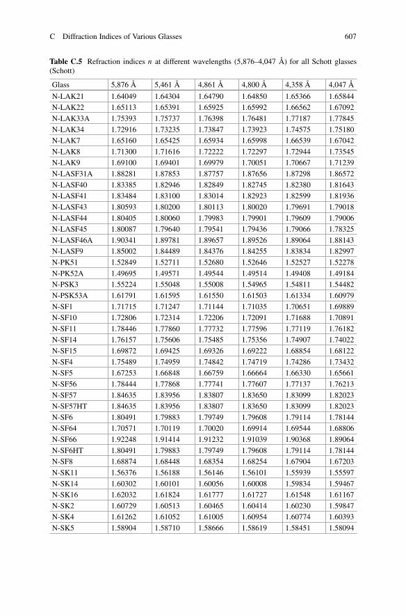
Table C.5 Refraction indices n at different wavelengths (5,876–4,047 Å) for all Schott glasses(Schott)
Glass 5,876 Å 5,461 Å 4,861 Å 4,800 Å 4,358 Å 4,047 Å
N-LAK21 1.64049 1.64304 1.64790 1.64850 1.65366 1.65844
N-LAK22 1.65113 1.65391 1.65925 1.65992 1.66562 1.67092
N-LAK33A 1.75393 1.75737 1.76398 1.76481 1.77187 1.77845
N-LAK34 1.72916 1.73235 1.73847 1.73923 1.74575 1.75180
N-LAK7 1.65160 1.65425 1.65934 1.65998 1.66539 1.67042
N-LAK8 1.71300 1.71616 1.72222 1.72297 1.72944 1.73545
N-LAK9 1.69100 1.69401 1.69979 1.70051 1.70667 1.71239
N-LASF31A 1.88281 1.87853 1.87757 1.87656 1.87298 1.86572
N-LASF40 1.83385 1.82946 1.82849 1.82745 1.82380 1.81643
N-LASF41 1.83484 1.83100 1.83014 1.82923 1.82599 1.81936
N-LASF43 1.80593 1.80200 1.80113 1.80020 1.79691 1.79018
N-LASF44 1.80405 1.80060 1.79983 1.79901 1.79609 1.79006
N-LASF45 1.80087 1.79640 1.79541 1.79436 1.79066 1.78325
N-LASF46A 1.90341 1.89781 1.89657 1.89526 1.89064 1.88143
N-LASF9 1.85002 1.84489 1.84376 1.84255 1.83834 1.82997
N-PK51 1.52849 1.52711 1.52680 1.52646 1.52527 1.52278
N-PK52A 1.49695 1.49571 1.49544 1.49514 1.49408 1.49184
N-PSK3 1.55224 1.55048 1.55008 1.54965 1.54811 1.54482
N-PSK53A 1.61791 1.61595 1.61550 1.61503 1.61334 1.60979
N-SF1 1.71715 1.71247 1.71144 1.71035 1.70651 1.69889
N-SF10 1.72806 1.72314 1.72206 1.72091 1.71688 1.70891
N-SF11 1.78446 1.77860 1.77732 1.77596 1.77119 1.76182
N-SF14 1.76157 1.75606 1.75485 1.75356 1.74907 1.74022
N-SF15 1.69872 1.69425 1.69326 1.69222 1.68854 1.68122
N-SF4 1.75489 1.74959 1.74842 1.74719 1.74286 1.73432
N-SF5 1.67253 1.66848 1.66759 1.66664 1.66330 1.65661
N-SF56 1.78444 1.77868 1.77741 1.77607 1.77137 1.76213
N-SF57 1.84635 1.83956 1.83807 1.83650 1.83099 1.82023
N-SF57HT 1.84635 1.83956 1.83807 1.83650 1.83099 1.82023
N-SF6 1.80491 1.79883 1.79749 1.79608 1.79114 1.78144
N-SF64 1.70571 1.70119 1.70020 1.69914 1.69544 1.68806
N-SF66 1.92248 1.91414 1.91232 1.91039 1.90368 1.89064
N-SF6HT 1.80491 1.79883 1.79749 1.79608 1.79114 1.78144
N-SF8 1.68874 1.68448 1.68354 1.68254 1.67904 1.67203
N-SK11 1.56376 1.56188 1.56146 1.56101 1.55939 1.55597
N-SK14 1.60302 1.60101 1.60056 1.60008 1.59834 1.59467
N-SK16 1.62032 1.61824 1.61777 1.61727 1.61548 1.61167
N-SK2 1.60729 1.60513 1.60465 1.60414 1.60230 1.59847
N-SK4 1.61262 1.61052 1.61005 1.60954 1.60774 1.60393
N-SK5 1.58904 1.58710 1.58666 1.58619 1.58451 1.58094
608 C Diffraction Indices of Various Glasses
Table C.6 Refraction indices n at different wavelengths (5,876–4,047 Å) for all Schott glasses(Schott)
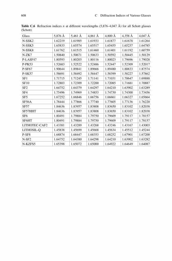
Glass 5,876 Å 5,461 Å 4,861 Å 4,800 Å 4,358 Å 4,047 Å
N-SSK2 1.62219 1.61985 1.61933 1.61877 1.61678 1.61264
N-SSK5 1.65833 1.65574 1.65517 1.65455 1.65237 1.64785
N-SSK8 1.61762 1.61515 1.61460 1.61401 1.61192 1.60759
N-ZK7 1.50840 1.50671 1.50633 1.50592 1.50445 1.50129
P-LASF47 1.80593 1.80203 1.80116 1.80023 1.79696 1.79028
P-PK53 1.52683 1.52522 1.52486 1.52447 1.52309 1.52017
P-SF67 1.90644 1.89841 1.89666 1.89480 1.88833 1.87574
P-SK57 1.58691 1.58492 1.58447 1.58399 1.58227 1.57862
SF1 1.71715 1.71245 1.71141 1.71031 1.70647 1.69888
SF10 1.72803 1.72309 1.72200 1.72085 1.71681 1.70887
SF2 1.64752 1.64379 1.64297 1.64210 1.63902 1.63289
SF4 1.75496 1.74969 1.74853 1.74730 1.74300 1.73456
SF5 1.67252 1.66846 1.66756 1.66661 1.66327 1.65664
SF56A 1.78444 1.77866 1.77740 1.77605 1.77136 1.76220
SF57 1.84636 1.83957 1.83808 1.83650 1.83102 1.82038
SF57HHT 1.84636 1.83957 1.83808 1.83650 1.83102 1.82038
SF6 1.80491 1.79884 1.79750 1.79609 1.79117 1.78157
SF6HT 1.80491 1.79884 1.79750 1.79609 1.79117 1.78157
LITHOTEC-CAF2 1.43381 1.43289 1.43268 1.43246 1.43167 1.43003
LITHOSIL-Q 1.45838 1.45699 1.45668 1.45634 1.45512 1.45244
P-SF8 1.68874 1.68447 1.68353 1.68252 1.67901 1.67200
N-SF2 1.64752 1.64380 1.64298 1.64210 1.63902 1.63282
N-KZFS5 1.65398 1.65072 1.65000 1.64922 1.64649 1.64087
Appendix DTransmissivity of Various Glasses
In a telescope-spectrograph system, light passes through a series of optical elements.As a result, the overall efficiency of standard spectrographs is of the order of 50 %,for echelle spectrographs even only 10 %. It is therefore essential to know theefficiency of all individual optical elements. Figure D.1 illustrates the refractionindices for all Schott glasses in the wavelength interval 4,000–8,500 Å (25 mmglass thickness). The corresponding values for specific wavelengths are shown inTables D.1, D.2, D.3, D.4, D.5, and D.6. The corresponding values for the entireinterval 2,500–25,000 Å are available from Schott or directly on their website.
© Springer-Verlag Berlin Heidelberg 2015T. Eversberg, K. Vollmann, Spectroscopic Instrumentation, Springer Praxis Books,DOI 10.1007/978-3-662-44535-8
609
610 D Transmissivity of Various Glasses
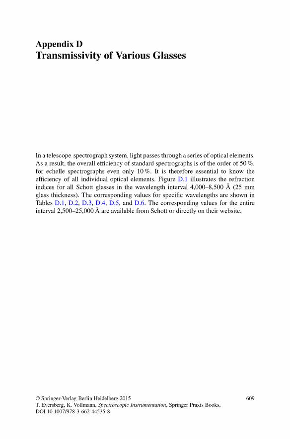
Fig. D.1 Graph of the transmissivity of all available Schott glass types (25 mm thickness) for thewavelength interval 4,000–8,500 Å (Schott). The majority of all glasses become opaque belowabout 500 nm. Only some glasses are transparent in UV wavelengths
D Transmissivity of Various Glasses 611
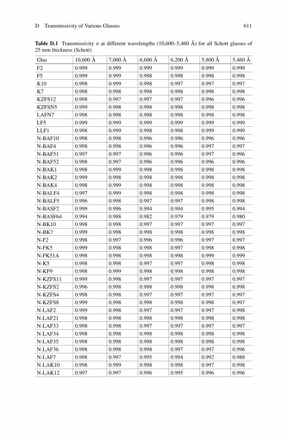
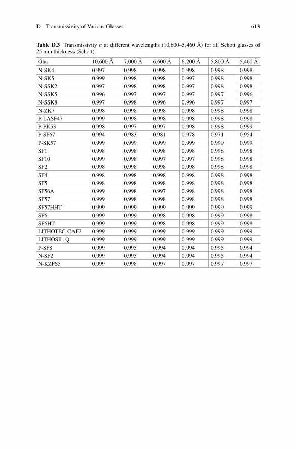
Table D.1 Transmissivity n at different wavelengths (10,600–5,460 Å) for all Schott glasses of25 mm thickness (Schott)
Glas 10,600 Å 7,000 Å 6,600 Å 6,200 Å 5,800 Å 5,460 Å
F2 0.999 0.999 0.999 0.999 0.999 0.999
F5 0.999 0.999 0.998 0.998 0.998 0.998
K10 0.998 0.999 0.998 0.997 0.997 0.997
K7 0.998 0.998 0.998 0.998 0.998 0.998
KZFS12 0.998 0.997 0.997 0.997 0.996 0.996
KZFSN5 0.999 0.998 0.998 0.998 0.998 0.998
LAFN7 0.998 0.998 0.998 0.998 0.998 0.998
LF5 0.999 0.999 0.999 0.999 0.999 0.999
LLF1 0.998 0.999 0.998 0.998 0.999 0.999
N-BAF10 0.998 0.998 0.996 0.996 0.996 0.996
N-BAF4 0.998 0.998 0.996 0.996 0.997 0.997
N-BAF51 0.997 0.997 0.996 0.996 0.997 0.996
N-BAF52 0.998 0.997 0.996 0.996 0.996 0.996
N-BAK1 0.998 0.999 0.998 0.998 0.998 0.998
N-BAK2 0.999 0.998 0.998 0.998 0.998 0.998
N-BAK4 0.998 0.999 0.998 0.998 0.998 0.998
N-BALF4 0.997 0.999 0.998 0.998 0.998 0.998
N-BALF5 0.996 0.998 0.997 0.997 0.998 0.998
N-BASF2 0.999 0.996 0.994 0.994 0.995 0.994
N-BASF64 0.994 0.988 0.982 0.979 0.979 0.980
N-BK10 0.998 0.998 0.997 0.997 0.997 0.997
N-BK7 0.999 0.998 0.998 0.998 0.998 0.998
N-F2 0.998 0.997 0.996 0.996 0.997 0.997
N-FK5 0.999 0.998 0.998 0.997 0.998 0.998
N-FK51A 0.998 0.998 0.998 0.998 0.999 0.999
N-K5 0.998 0.998 0.997 0.997 0.998 0.998
N-KF9 0.998 0.999 0.998 0.998 0.998 0.998
N-KZFS11 0.999 0.998 0.997 0.997 0.997 0.997
N-KZFS2 0.996 0.998 0.998 0.998 0.998 0.998
N-KZFS4 0.998 0.998 0.997 0.997 0.997 0.997
N-KZFS8 0.999 0.998 0.998 0.998 0.998 0.997
N-LAF2 0.999 0.998 0.997 0.997 0.997 0.998
N-LAF21 0.998 0.998 0.998 0.998 0.998 0.998
N-LAF33 0.998 0.998 0.997 0.997 0.997 0.997
N-LAF34 0.998 0.998 0.998 0.998 0.998 0.998
N-LAF35 0.998 0.998 0.998 0.998 0.998 0.998
N-LAF36 0.998 0.998 0.998 0.997 0.997 0.996
N-LAF7 0.998 0.997 0.995 0.994 0.992 0.988
N-LAK10 0.998 0.999 0.998 0.998 0.997 0.998
N-LAK12 0.997 0.997 0.996 0.995 0.996 0.996
612 D Transmissivity of Various Glasses
Table D.2 Transmissivity n at different wavelengths (10,600–5,460 Å) for all Schott glasses of25 mm thickness (Schott)
Glas 10,600 Å 7,000 Å 6,600 Å 6,200 Å 5,800 Å 5,460 Å
N-LAK14 0.998 0.998 0.998 0.997 0.997 0.998
N-LAK21 0.998 0.998 0.996 0.996 0.997 0.997
N-LAK22 0.998 0.998 0.997 0.996 0.997 0.997
N-LAK33A 0.998 0.998 0.998 0.998 0.998 0.998
N-LAK34 0.998 0.999 0.999 0.998 0.998 0.999
N-LAK7 0.998 0.998 0.998 0.998 0.998 0.998
N-LAK8 0.998 0.998 0.998 0.998 0.998 0.998
N-LAK9 0.998 0.998 0.998 0.998 0.998 0.998
N-LASF31A 0.996 0.996 0.995 0.994 0.995 0.994
N-LASF40 0.998 0.998 0.998 0.997 0.997 0.995
N-LASF41 0.998 0.998 0.998 0.997 0.998 0.997
N-LASF43 0.998 0.998 0.998 0.997 0.996 0.995
N-LASF44 0.998 0.998 0.998 0.998 0.998 0.998
N-LASF45 0.997 0.997 0.995 0.994 0.994 0.993
N-LASF46A 0.999 0.996 0.994 0.993 0.993 0.991
N-LASF9 0.998 0.995 0.994 0.993 0.992 0.990
N-PK51 0.998 0.997 0.996 0.997 0.998 0.998
N-PK52A 0.998 0.997 0.997 0.998 0.999 0.999
N-PSK3 0.999 0.998 0.997 0.997 0.997 0.997
N-PSK53 0.998 0.998 0.997 0.997 0.998 0.998
N-PSK53A 0.998 0.998 0.997 0.997 0.998 0.998
N-SF1 0.998 0.996 0.994 0.995 0.996 0.994
N-SF10 0.996 0.993 0.990 0.991 0.991 0.989
N-SF11 0.999 0.994 0.992 0.992 0.994 0.991
N-SF14 0.999 0.994 0.991 0.992 0.994 0.992
N-SF15 0.998 0.995 0.993 0.994 0.994 0.994
N-SF4 0.999 0.995 0.993 0.993 0.993 0.990
N-SF5 0.998 0.996 0.995 0.995 0.996 0.995
N-SF56 0.998 0.994 0.992 0.992 0.993 0.990
N-SF57 0.999 0.991 0.987 0.988 0.990 0.986
N-SF57HT 0.999 0.992 0.988 0.989 0.991 0.987
N-SF6 0.998 0.993 0.991 0.991 0.992 0.989
N-SF64 0.998 0.994 0.992 0.992 0.994 0.993
N-SF66 0.996 0.991 0.987 0.983 0.976 0.963
N-SF6HT 0.999 0.994 0.991 0.992 0.992 0.990
N-SF8 0.997 0.995 0.993 0.993 0.994 0.993
N-SK11 0.998 0.998 0.998 0.998 0.998 0.999
N-SK14 0.998 0.998 0.998 0.998 0.998 0.998
N-SK16 0.998 0.998 0.998 0.997 0.998 0.998
N-SK2 0.998 0.998 0.998 0.998 0.998 0.998
D Transmissivity of Various Glasses 613
Table D.3 Transmissivity n at different wavelengths (10,600–5,460 Å) for all Schott glasses of25 mm thickness (Schott)
Glas 10,600 Å 7,000 Å 6,600 Å 6,200 Å 5,800 Å 5,460 Å
N-SK4 0.997 0.998 0.998 0.998 0.998 0.998
N-SK5 0.999 0.998 0.998 0.997 0.998 0.998
N-SSK2 0.997 0.998 0.998 0.997 0.998 0.998
N-SSK5 0.996 0.997 0.997 0.997 0.997 0.996
N-SSK8 0.997 0.998 0.996 0.996 0.997 0.997
N-ZK7 0.998 0.998 0.998 0.998 0.998 0.998
P-LASF47 0.999 0.998 0.998 0.998 0.998 0.998
P-PK53 0.998 0.997 0.997 0.998 0.998 0.999
P-SF67 0.994 0.983 0.981 0.978 0.971 0.954
P-SK57 0.999 0.999 0.999 0.999 0.999 0.999
SF1 0.998 0.998 0.998 0.998 0.998 0.998
SF10 0.999 0.998 0.997 0.997 0.998 0.998
SF2 0.998 0.998 0.998 0.998 0.998 0.998
SF4 0.998 0.998 0.998 0.998 0.998 0.998
SF5 0.998 0.998 0.998 0.998 0.998 0.998
SF56A 0.999 0.998 0.997 0.998 0.998 0.998
SF57 0.999 0.998 0.998 0.998 0.998 0.998
SF57HHT 0.999 0.999 0.999 0.999 0.999 0.999
SF6 0.999 0.999 0.998 0.998 0.999 0.998
SF6HT 0.999 0.999 0.998 0.998 0.999 0.998
LITHOTEC-CAF2 0.999 0.999 0.999 0.999 0.999 0.999
LITHOSIL-Q 0.999 0.999 0.999 0.999 0.999 0.999
P-SF8 0.999 0.995 0.994 0.994 0.995 0.994
N-SF2 0.999 0.995 0.994 0.994 0.995 0.994
N-KZFS5 0.999 0.998 0.997 0.997 0.997 0.997
614 D Transmissivity of Various Glasses
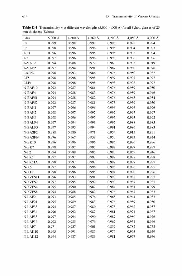
Table D.4 Transmissivity n at different wavelengths (5,000–4,000 Å) for all Schott glasses of 25mm thickness (Schott)
Glas 5,000 Å 4,600 Å 4,360 Å 4,200 Å 4,050 Å 4,000 Å
F2 0.999 0.998 0.997 0.996 0.995 0.994
F5 0.998 0.996 0.996 0.995 0.994 0.993
K10 0.996 0.996 0.995 0.995 0.995 0.994
K7 0.997 0.996 0.996 0.996 0.996 0.996
KZFS12 0.994 0.988 0.977 0.963 0.933 0.919
KZFSN5 0.997 0.994 0.991 0.987 0.980 0.976
LAFN7 0.998 0.993 0.986 0.976 0.950 0.937
LF5 0.998 0.998 0.998 0.997 0.997 0.997
LLF1 0.998 0.998 0.998 0.998 0.998 0.997
N-BAF10 0.992 0.987 0.981 0.976 0.959 0.950
N-BAF4 0.994 0.988 0.983 0.976 0.959 0.946
N-BAF51 0.994 0.988 0.982 0.976 0.963 0.954
N-BAF52 0.992 0.987 0.981 0.975 0.959 0.950
N-BAK1 0.997 0.996 0.996 0.996 0.996 0.996
N-BAK2 0.998 0.997 0.997 0.997 0.997 0.997
N-BAK4 0.998 0.996 0.995 0.995 0.993 0.992
N-BALF4 0.997 0.994 0.993 0.992 0.988 0.985
N-BALF5 0.997 0.995 0.994 0.991 0.986 0.983
N-BASF2 0.988 0.980 0.971 0.954 0.915 0.891
N-BASF64 0.976 0.967 0.959 0.950 0.933 0.924
N-BK10 0.996 0.996 0.996 0.996 0.996 0.996
N-BK7 0.998 0.997 0.997 0.997 0.997 0.997
N-F2 0.994 0.989 0.985 0.980 0.959 0.946
N-FK5 0.997 0.997 0.997 0.997 0.998 0.998
N-FK51A 0.998 0.997 0.997 0.997 0.997 0.997
N-K5 0.997 0.996 0.996 0.996 0.996 0.995
N-KF9 0.998 0.996 0.995 0.994 0.990 0.986
N-KZFS11 0.996 0.993 0.991 0.990 0.988 0.987
N-KZFS2 0.997 0.995 0.992 0.990 0.987 0.985
N-KZFS4 0.995 0.990 0.987 0.984 0.981 0.979
N-KZFS8 0.994 0.988 0.982 0.976 0.967 0.963
N-LAF2 0.993 0.985 0.976 0.965 0.944 0.933
N-LAF21 0.995 0.989 0.983 0.976 0.959 0.950
N-LAF33 0.994 0.987 0.980 0.973 0.962 0.957
N-LAF34 0.996 0.992 0.987 0.981 0.971 0.967
N-LAF35 0.997 0.994 0.990 0.987 0.980 0.976
N-LAF36 0.992 0.985 0.976 0.967 0.954 0.946
N-LAF7 0.971 0.937 0.901 0.857 0.782 0.752
N-LAK10 0.995 0.991 0.985 0.976 0.963 0.959
N-LAK12 0.994 0.987 0.983 0.981 0.977 0.976
D Transmissivity of Various Glasses 615
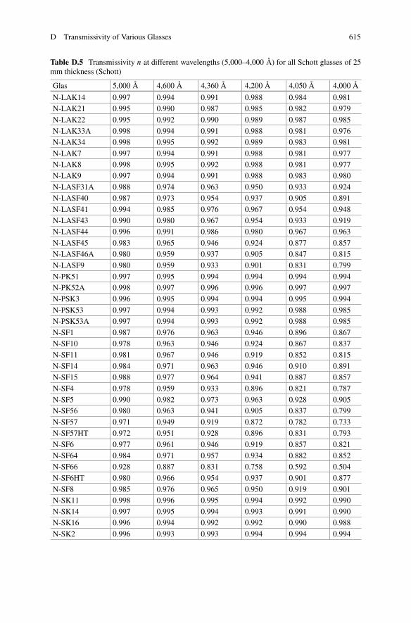
Table D.5 Transmissivity n at different wavelengths (5,000–4,000 Å) for all Schott glasses of 25mm thickness (Schott)
Glas 5,000 Å 4,600 Å 4,360 Å 4,200 Å 4,050 Å 4,000 Å
N-LAK14 0.997 0.994 0.991 0.988 0.984 0.981
N-LAK21 0.995 0.990 0.987 0.985 0.982 0.979
N-LAK22 0.995 0.992 0.990 0.989 0.987 0.985
N-LAK33A 0.998 0.994 0.991 0.988 0.981 0.976
N-LAK34 0.998 0.995 0.992 0.989 0.983 0.981
N-LAK7 0.997 0.994 0.991 0.988 0.981 0.977
N-LAK8 0.998 0.995 0.992 0.988 0.981 0.977
N-LAK9 0.997 0.994 0.991 0.988 0.983 0.980
N-LASF31A 0.988 0.974 0.963 0.950 0.933 0.924
N-LASF40 0.987 0.973 0.954 0.937 0.905 0.891
N-LASF41 0.994 0.985 0.976 0.967 0.954 0.948
N-LASF43 0.990 0.980 0.967 0.954 0.933 0.919
N-LASF44 0.996 0.991 0.986 0.980 0.967 0.963
N-LASF45 0.983 0.965 0.946 0.924 0.877 0.857
N-LASF46A 0.980 0.959 0.937 0.905 0.847 0.815
N-LASF9 0.980 0.959 0.933 0.901 0.831 0.799
N-PK51 0.997 0.995 0.994 0.994 0.994 0.994
N-PK52A 0.998 0.997 0.996 0.996 0.997 0.997
N-PSK3 0.996 0.995 0.994 0.994 0.995 0.994
N-PSK53 0.997 0.994 0.993 0.992 0.988 0.985
N-PSK53A 0.997 0.994 0.993 0.992 0.988 0.985
N-SF1 0.987 0.976 0.963 0.946 0.896 0.867
N-SF10 0.978 0.963 0.946 0.924 0.867 0.837
N-SF11 0.981 0.967 0.946 0.919 0.852 0.815
N-SF14 0.984 0.971 0.963 0.946 0.910 0.891
N-SF15 0.988 0.977 0.964 0.941 0.887 0.857
N-SF4 0.978 0.959 0.933 0.896 0.821 0.787
N-SF5 0.990 0.982 0.973 0.963 0.928 0.905
N-SF56 0.980 0.963 0.941 0.905 0.837 0.799
N-SF57 0.971 0.949 0.919 0.872 0.782 0.733
N-SF57HT 0.972 0.951 0.928 0.896 0.831 0.793
N-SF6 0.977 0.961 0.946 0.919 0.857 0.821
N-SF64 0.984 0.971 0.957 0.934 0.882 0.852
N-SF66 0.928 0.887 0.831 0.758 0.592 0.504
N-SF6HT 0.980 0.966 0.954 0.937 0.901 0.877
N-SF8 0.985 0.976 0.965 0.950 0.919 0.901
N-SK11 0.998 0.996 0.995 0.994 0.992 0.990
N-SK14 0.997 0.995 0.994 0.993 0.991 0.990
N-SK16 0.996 0.994 0.992 0.992 0.990 0.988
N-SK2 0.996 0.993 0.993 0.994 0.994 0.994
616 D Transmissivity of Various Glasses
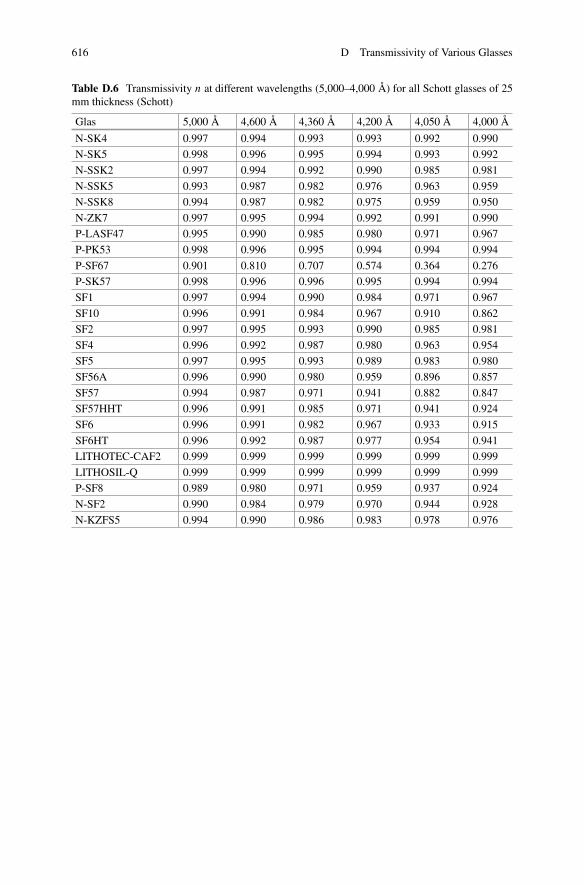
Table D.6 Transmissivity n at different wavelengths (5,000–4,000 Å) for all Schott glasses of 25mm thickness (Schott)
Glas 5,000 Å 4,600 Å 4,360 Å 4,200 Å 4,050 Å 4,000 Å
N-SK4 0.997 0.994 0.993 0.993 0.992 0.990
N-SK5 0.998 0.996 0.995 0.994 0.993 0.992
N-SSK2 0.997 0.994 0.992 0.990 0.985 0.981
N-SSK5 0.993 0.987 0.982 0.976 0.963 0.959
N-SSK8 0.994 0.987 0.982 0.975 0.959 0.950
N-ZK7 0.997 0.995 0.994 0.992 0.991 0.990
P-LASF47 0.995 0.990 0.985 0.980 0.971 0.967
P-PK53 0.998 0.996 0.995 0.994 0.994 0.994
P-SF67 0.901 0.810 0.707 0.574 0.364 0.276
P-SK57 0.998 0.996 0.996 0.995 0.994 0.994
SF1 0.997 0.994 0.990 0.984 0.971 0.967
SF10 0.996 0.991 0.984 0.967 0.910 0.862
SF2 0.997 0.995 0.993 0.990 0.985 0.981
SF4 0.996 0.992 0.987 0.980 0.963 0.954
SF5 0.997 0.995 0.993 0.989 0.983 0.980
SF56A 0.996 0.990 0.980 0.959 0.896 0.857
SF57 0.994 0.987 0.971 0.941 0.882 0.847
SF57HHT 0.996 0.991 0.985 0.971 0.941 0.924
SF6 0.996 0.991 0.982 0.967 0.933 0.915
SF6HT 0.996 0.992 0.987 0.977 0.954 0.941
LITHOTEC-CAF2 0.999 0.999 0.999 0.999 0.999 0.999
LITHOSIL-Q 0.999 0.999 0.999 0.999 0.999 0.999
P-SF8 0.989 0.980 0.971 0.959 0.937 0.924
N-SF2 0.990 0.984 0.979 0.970 0.944 0.928
N-KZFS5 0.994 0.990 0.986 0.983 0.978 0.976
Appendix ELine Catalogues for Calibration Lamps
E.1 Line Catalogue Sources
• THORIUM-ARGON Line CatalogueFOCES High Resolution Echelle Spectra at 2.2 m Calar Altohttp://www.caha.es/pedraz/Foces/thar_lamp.html
• NOAO SPECTRAL ATLASThAr Photron Lamp at 2.1 m KPNOhttp://www.noao.edu/kpno/specatlas/thar_photron/thar_photron.html
• NOAO SPECTRAL ATLASThAr Westinghouse Lamp at 2.1 m KPNOhttp://www.noao.edu/kpno/specatlas/thar/thar.html
• NOAO SPECTRAL ATLASFeAr Lamp at 2.1 m KPNOhttp://www.noao.edu/kpno/specatlas/fear/fear.html
• NOAO SPECTRAL ATLASHeNe Lamp at 2.1 m KPNOhttp://www.noao.edu/kpno/specatlas/henear/henear.html
• NOAO SPECTRAL ATLASCuAr Lamp at 2.1 m KPNOhttp://www.noao.edu/kpno/specatlas/cuar/cuar.html
• High Resolution Line AtlasHe-Ar-Fe-Ne Lamp at ESO 1.5 mhttp://www.ls.eso.org/lasilla/Telescopes/2p2T/E1p5M/memos_notes/Line-atlas-feros.html
• CFHT Coudé Comparison Arc Spectral AtlasesThAr, FeAr, CdNe and ThNe Lamps at 3.6 m CFHThttp://www.cfht.hawaii.edu/Instruments/Spectroscopy/Gecko/CoudeAtlas/
© Springer-Verlag Berlin Heidelberg 2015T. Eversberg, K. Vollmann, Spectroscopic Instrumentation, Springer Praxis Books,DOI 10.1007/978-3-662-44535-8
617
618 E Line Catalogues for Calibration Lamps
• HET HRS Th-Ar and Echelle Tilt AtlasTh-Ar Lamp at 9 m Hobby-Eberly Telescopehttp://het.as.utexas.edu/HET/hetweb/Instruments/HRS/hrs_thar.html
E.2 Line Catalogue for the Glow Starter RELCO SC480
A visible spectrum of the RELCO SC480 low-cost glow starter1 has been obtainedwith an off-the-shelf SQUES echelle spectrograph (Huwiler 2014) at R � 20,000.The wavelength range of 3,888–8,136 Å is distributed over 30 echelle orders. 2D-spectra are shown in Figs. E.1, E.2, and E.3. All usable emission lines are indicatedin Figs. E.4, E.5, E.6, E.7, E.8, and E.9 (some lines occur twice due to overlappingorders. Their wavelengths are labeled in different colours). The correspondingcatalogue is shown in Tables E.1, E.2, E.3, E.4 and E.5. In order 29 (7,600–7,900Å), only two usable emission lines are generated by noble gases. However, they aresupplemented by a strong oxygen triplet. Line pairs which appear scarcely resolvedare referred to as a “blend”.
1The off-the-shelf RELCO starter costs only some cents.
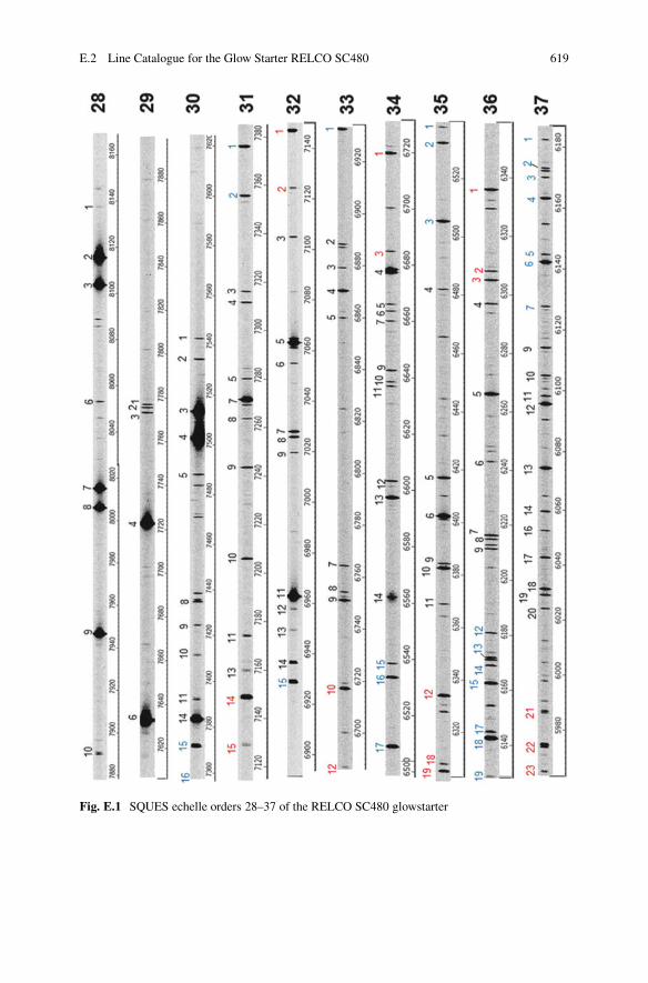
E.2 Line Catalogue for the Glow Starter RELCO SC480 619
Fig. E.1 SQUES echelle orders 28–37 of the RELCO SC480 glowstarter
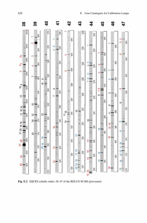
620 E Line Catalogues for Calibration Lamps
Fig. E.2 SQUES echelle orders 38–47 of the RELCO SC480 glowstarter
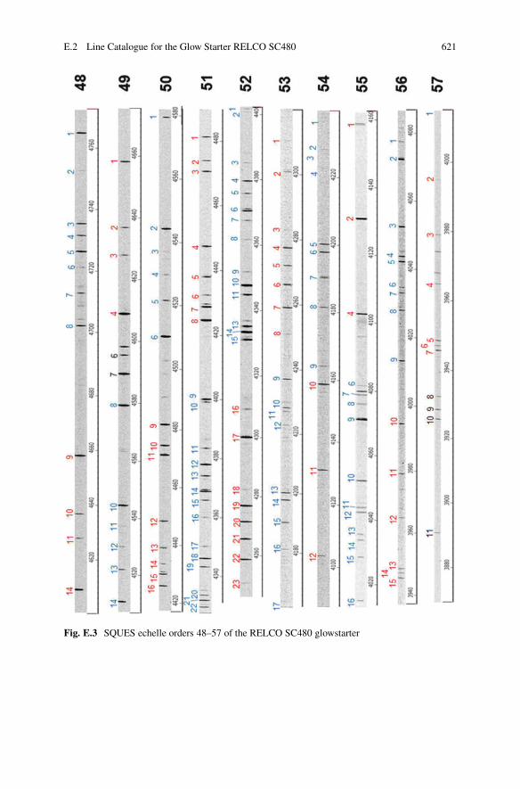
E.2 Line Catalogue for the Glow Starter RELCO SC480 621
Fig. E.3 SQUES echelle orders 48–57 of the RELCO SC480 glowstarter
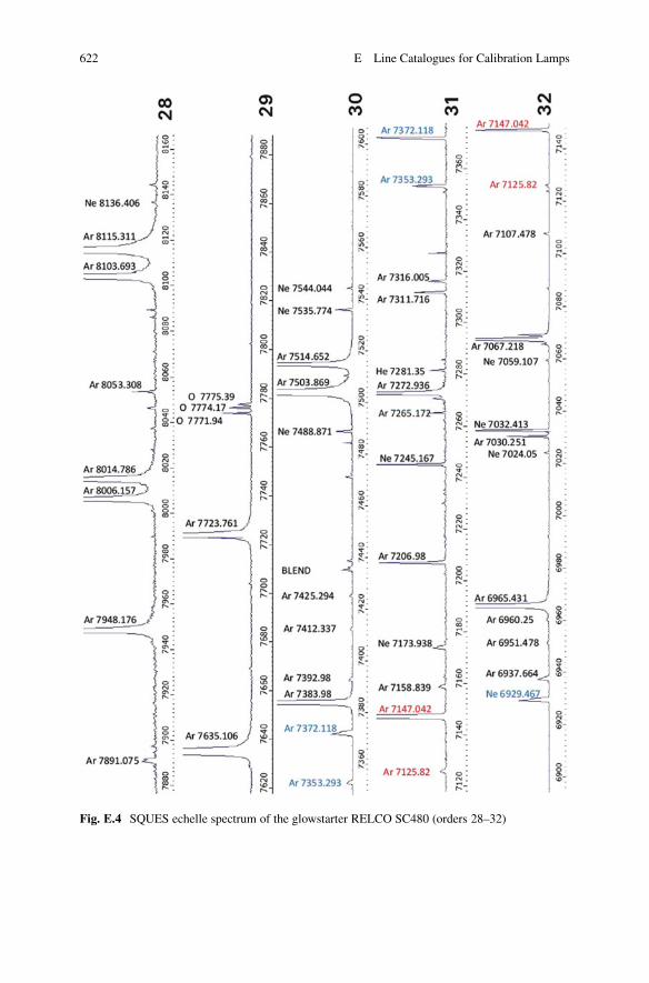
622 E Line Catalogues for Calibration Lamps
Fig. E.4 SQUES echelle spectrum of the glowstarter RELCO SC480 (orders 28–32)
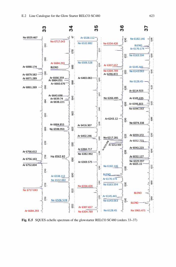
E.2 Line Catalogue for the Glow Starter RELCO SC480 623
Fig. E.5 SQUES echelle spectrum of the glowstarter RELCO SC480 (orders 33–37)
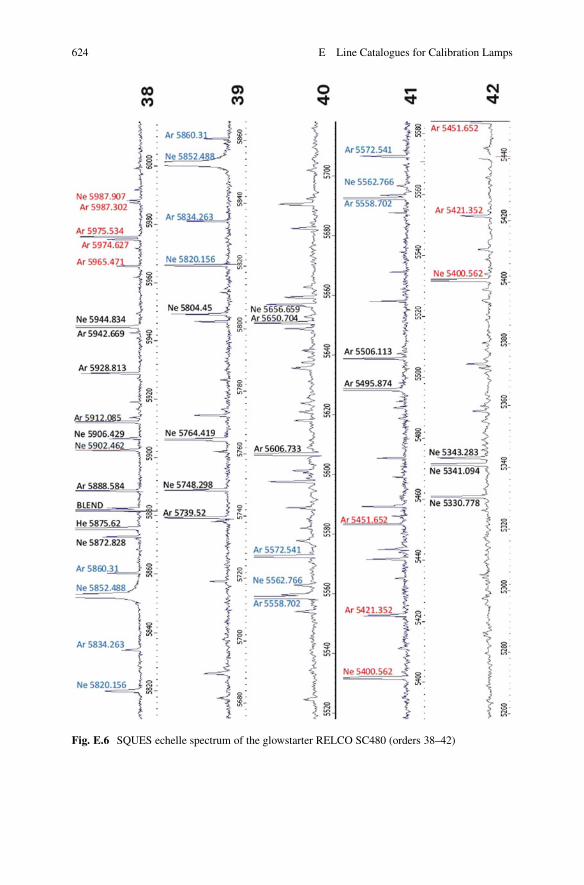
624 E Line Catalogues for Calibration Lamps
Fig. E.6 SQUES echelle spectrum of the glowstarter RELCO SC480 (orders 38–42)
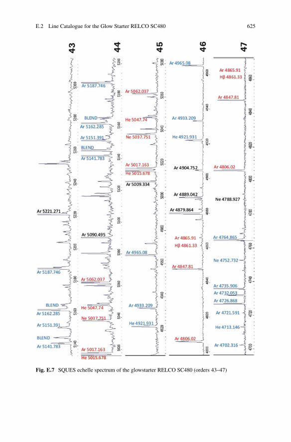
E.2 Line Catalogue for the Glow Starter RELCO SC480 625
Fig. E.7 SQUES echelle spectrum of the glowstarter RELCO SC480 (orders 43–47)
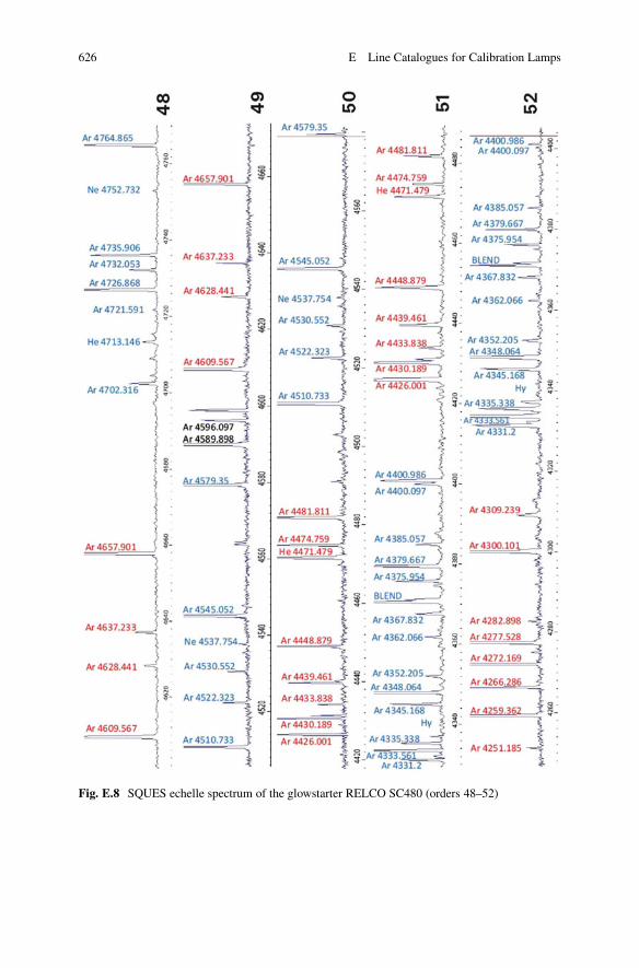
626 E Line Catalogues for Calibration Lamps
Fig. E.8 SQUES echelle spectrum of the glowstarter RELCO SC480 (orders 48–52)
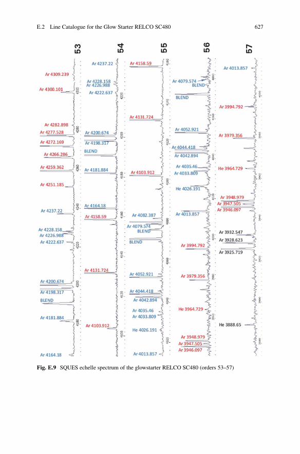
E.2 Line Catalogue for the Glow Starter RELCO SC480 627
Fig. E.9 SQUES echelle spectrum of the glowstarter RELCO SC480 (orders 53–57)
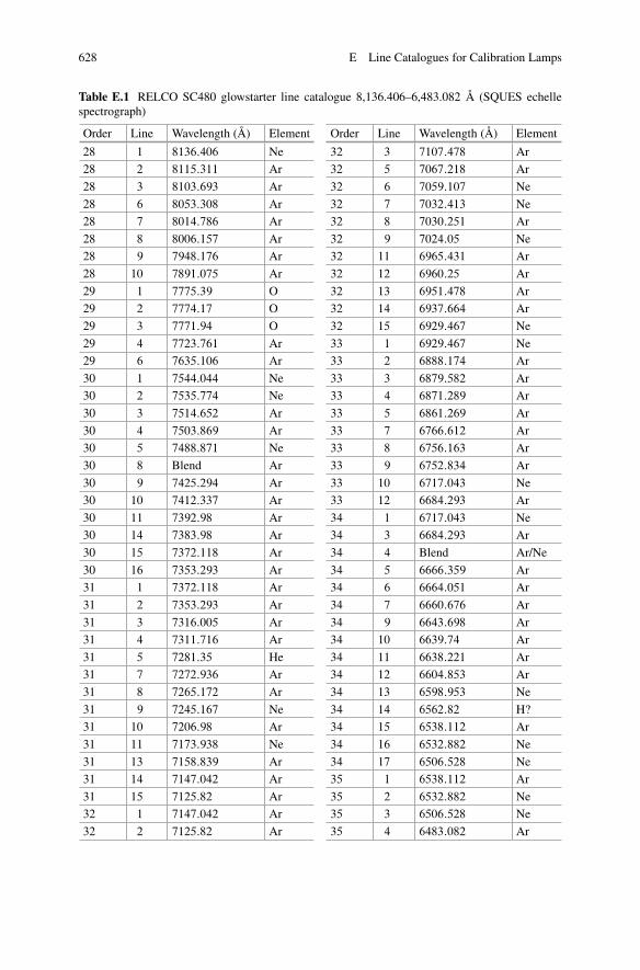
628 E Line Catalogues for Calibration Lamps
Table E.1 RELCO SC480 glowstarter line catalogue 8,136.406–6,483.082 Å (SQUES echellespectrograph)
Order Line Wavelength (Å) Element
28 1 8136:406 Ne
28 2 8115:311 Ar
28 3 8103:693 Ar
28 6 8053:308 Ar
28 7 8014:786 Ar
28 8 8006:157 Ar
28 9 7948:176 Ar
28 10 7891:075 Ar
29 1 7775:39 O
29 2 7774:17 O
29 3 7771:94 O
29 4 7723:761 Ar
29 6 7635:106 Ar
30 1 7544:044 Ne
30 2 7535:774 Ne
30 3 7514:652 Ar
30 4 7503:869 Ar
30 5 7488:871 Ne
30 8 Blend Ar
30 9 7425:294 Ar
30 10 7412:337 Ar
30 11 7392:98 Ar
30 14 7383:98 Ar
30 15 7372:118 Ar
30 16 7353:293 Ar
31 1 7372:118 Ar
31 2 7353:293 Ar
31 3 7316:005 Ar
31 4 7311:716 Ar
31 5 7281:35 He
31 7 7272:936 Ar
31 8 7265:172 Ar
31 9 7245:167 Ne
31 10 7206:98 Ar
31 11 7173:938 Ne
31 13 7158:839 Ar
31 14 7147:042 Ar
31 15 7125:82 Ar
32 1 7147:042 Ar
32 2 7125:82 Ar
Order Line Wavelength (Å) Element
32 3 7107:478 Ar
32 5 7067:218 Ar
32 6 7059:107 Ne
32 7 7032:413 Ne
32 8 7030:251 Ar
32 9 7024:05 Ne
32 11 6965:431 Ar
32 12 6960:25 Ar
32 13 6951:478 Ar
32 14 6937:664 Ar
32 15 6929:467 Ne
33 1 6929:467 Ne
33 2 6888:174 Ar
33 3 6879:582 Ar
33 4 6871:289 Ar
33 5 6861:269 Ar
33 7 6766:612 Ar
33 8 6756:163 Ar
33 9 6752:834 Ar
33 10 6717:043 Ne
33 12 6684:293 Ar
34 1 6717:043 Ne
34 3 6684:293 Ar
34 4 Blend Ar/Ne
34 5 6666:359 Ar
34 6 6664:051 Ar
34 7 6660:676 Ar
34 9 6643:698 Ar
34 10 6639:74 Ar
34 11 6638:221 Ar
34 12 6604:853 Ar
34 13 6598:953 Ne
34 14 6562:82 H?
34 15 6538:112 Ar
34 16 6532:882 Ne
34 17 6506:528 Ne
35 1 6538:112 Ar
35 2 6532:882 Ne
35 3 6506:528 Ne
35 4 6483:082 Ar
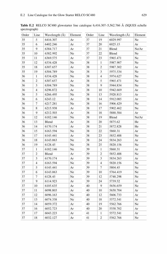
E.2 Line Catalogue for the Glow Starter RELCO SC480 629
Table E.2 RELCO SC480 glowstarter line catalogue 6,416.307–5,562.766 Å (SQUES echellespectrograph)
Order Line Wavelength (Å) Element
35 5 6416:307 Ar
35 6 6402:246 Ar
35 9 6384:717 Ar
35 10 6382:992 Ne
35 11 6369:575 Ar
35 12 6334:428 Ne
35 18 6307:657 Ar
35 19 6304:789 Ne
36 1 6334:428 Ne
36 2 6307:657 Ar
36 3 6304:789 Ne
36 4 6296:872 Ar
36 5 6266:495 Ne
36 6 6243:12 Ar
36 7 6217:281 Ne
36 8 6215:938 Ar
36 9 6212:503 Ar
36 12 6182:146 Ne
36 13 Blend Ar
36 14 6170:174 Ar
36 15 6163:594 Ne
36 17 6145:441 Ar
36 18 6143:063 Ne
36 19 6128:45 Ne
37 1 6182:146 Ne
37 2 Blend Ar
37 3 6170:174 Ar
37 4 6163:594 Ne
37 5 6145:441 Ar
37 6 6143:063 Ne
37 7 6128:45 Ne
37 9 6114:923 Ar
37 10 6105:635 Ar
37 11 6098:803 Ar
37 12 6096:163 Ne
37 13 6074:338 Ne
37 14 6059:372 Ar
37 16 6052:723 Ar
37 17 6043:223 Ar
37 18 6032:127 Ar
Order Line Wavelength (Å) Element
37 19 6029:997 Ne
37 20 6025:15 Ar
37 21 Blend Ne/Ar
37 22 Blend Ne
37 23 5965:471 Ne
38 1 5987:907 Ne
38 2 5987:302 Ar
38 3 5975:534 Ne
38 4 5974:627 Ne
38 5 5965:471 Ne
38 9 5944:834 Ne
38 10 5942:669 Ar
38 13 5928:813 Ar
38 14 5912:085 Ar
38 16 5906:429 Ne
38 17 5902:462 Ne
38 18 5888:584 Ar
38 19 Blend Ne/Ar
38 20 5875:62 He
38 21 5872:828 He
38 22 5860:31 Ar
38 23 5852:488 Ne
38 24 5834:263 Ar
38 25 5820:156 Ne
39 1 5860:31 Ar
39 2 5852:488 Ne
39 3 5834:263 Ar
39 4 5820:156 Ne
39 7 5804:45 Ne
39 10 5764:419 Ne
39 12 5748:298 Ne
39 24 5739:52 Ar
40 9 5656:659 Ne
40 10 5650:704 Ar
40 12 5606:733 Ar
40 18 5572:541 Ar
40 19 5562:766 Ne
40 20 5558:702 Ar
41 1 5572:541 Ar
41 2 5562:766 Ne
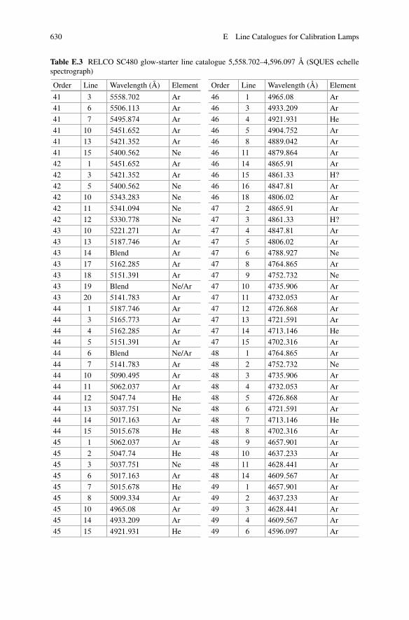
630 E Line Catalogues for Calibration Lamps
Table E.3 RELCO SC480 glow-starter line catalogue 5,558.702–4,596.097 Å (SQUES echellespectrograph)
Order Line Wavelength (Å) Element
41 3 5558:702 Ar
41 6 5506:113 Ar
41 7 5495:874 Ar
41 10 5451:652 Ar
41 13 5421:352 Ar
41 15 5400:562 Ne
42 1 5451:652 Ar
42 3 5421:352 Ar
42 5 5400:562 Ne
42 10 5343:283 Ne
42 11 5341:094 Ne
42 12 5330:778 Ne
43 10 5221:271 Ar
43 13 5187:746 Ar
43 14 Blend Ar
43 17 5162:285 Ar
43 18 5151:391 Ar
43 19 Blend Ne/Ar
43 20 5141:783 Ar
44 1 5187:746 Ar
44 3 5165:773 Ar
44 4 5162:285 Ar
44 5 5151:391 Ar
44 6 Blend Ne/Ar
44 7 5141:783 Ar
44 10 5090:495 Ar
44 11 5062:037 Ar
44 12 5047:74 He
44 13 5037:751 Ne
44 14 5017:163 Ar
44 15 5015:678 He
45 1 5062:037 Ar
45 2 5047:74 He
45 3 5037:751 Ne
45 6 5017:163 Ar
45 7 5015:678 He
45 8 5009:334 Ar
45 10 4965:08 Ar
45 14 4933:209 Ar
45 15 4921:931 He
Order Line Wavelength (Å) Element
46 1 4965:08 Ar
46 3 4933:209 Ar
46 4 4921:931 He
46 5 4904:752 Ar
46 8 4889:042 Ar
46 11 4879:864 Ar
46 14 4865:91 Ar
46 15 4861:33 H?
46 16 4847:81 Ar
46 18 4806:02 Ar
47 2 4865:91 Ar
47 3 4861:33 H?
47 4 4847:81 Ar
47 5 4806:02 Ar
47 6 4788:927 Ne
47 8 4764:865 Ar
47 9 4752:732 Ne
47 10 4735:906 Ar
47 11 4732:053 Ar
47 12 4726:868 Ar
47 13 4721:591 Ar
47 14 4713:146 He
47 15 4702:316 Ar
48 1 4764:865 Ar
48 2 4752:732 Ne
48 3 4735:906 Ar
48 4 4732:053 Ar
48 5 4726:868 Ar
48 6 4721:591 Ar
48 7 4713:146 He
48 8 4702:316 Ar
48 9 4657:901 Ar
48 10 4637:233 Ar
48 11 4628:441 Ar
48 14 4609:567 Ar
49 1 4657:901 Ar
49 2 4637:233 Ar
49 3 4628:441 Ar
49 4 4609:567 Ar
49 6 4596:097 Ar
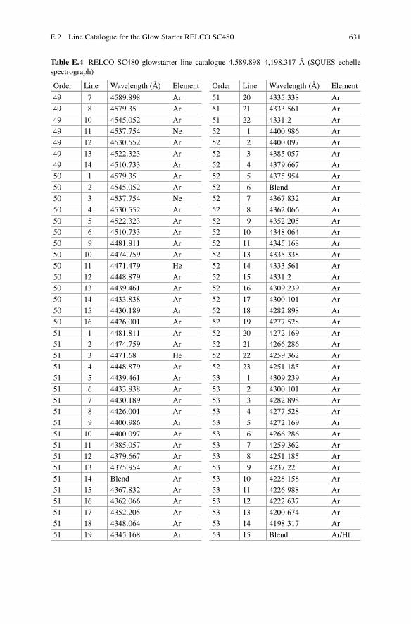
E.2 Line Catalogue for the Glow Starter RELCO SC480 631
Table E.4 RELCO SC480 glowstarter line catalogue 4,589.898–4,198.317 Å (SQUES echellespectrograph)
Order Line Wavelength (Å) Element
49 7 4589:898 Ar
49 8 4579:35 Ar
49 10 4545:052 Ar
49 11 4537:754 Ne
49 12 4530:552 Ar
49 13 4522:323 Ar
49 14 4510:733 Ar
50 1 4579:35 Ar
50 2 4545:052 Ar
50 3 4537:754 Ne
50 4 4530:552 Ar
50 5 4522:323 Ar
50 6 4510:733 Ar
50 9 4481:811 Ar
50 10 4474:759 Ar
50 11 4471:479 He
50 12 4448:879 Ar
50 13 4439:461 Ar
50 14 4433:838 Ar
50 15 4430:189 Ar
50 16 4426:001 Ar
51 1 4481:811 Ar
51 2 4474:759 Ar
51 3 4471:68 He
51 4 4448:879 Ar
51 5 4439:461 Ar
51 6 4433:838 Ar
51 7 4430:189 Ar
51 8 4426:001 Ar
51 9 4400:986 Ar
51 10 4400:097 Ar
51 11 4385:057 Ar
51 12 4379:667 Ar
51 13 4375:954 Ar
51 14 Blend Ar
51 15 4367:832 Ar
51 16 4362:066 Ar
51 17 4352:205 Ar
51 18 4348:064 Ar
51 19 4345:168 Ar
Order Line Wavelength (Å) Element
51 20 4335:338 Ar
51 21 4333:561 Ar
51 22 4331:2 Ar
52 1 4400:986 Ar
52 2 4400:097 Ar
52 3 4385:057 Ar
52 4 4379:667 Ar
52 5 4375:954 Ar
52 6 Blend Ar
52 7 4367:832 Ar
52 8 4362:066 Ar
52 9 4352:205 Ar
52 10 4348:064 Ar
52 11 4345:168 Ar
52 13 4335:338 Ar
52 14 4333:561 Ar
52 15 4331:2 Ar
52 16 4309:239 Ar
52 17 4300:101 Ar
52 18 4282:898 Ar
52 19 4277:528 Ar
52 20 4272:169 Ar
52 21 4266:286 Ar
52 22 4259:362 Ar
52 23 4251:185 Ar
53 1 4309:239 Ar
53 2 4300:101 Ar
53 3 4282:898 Ar
53 4 4277:528 Ar
53 5 4272:169 Ar
53 6 4266:286 Ar
53 7 4259:362 Ar
53 8 4251:185 Ar
53 9 4237:22 Ar
53 10 4228:158 Ar
53 11 4226:988 Ar
53 12 4222:637 Ar
53 13 4200:674 Ar
53 14 4198:317 Ar
53 15 Blend Ar/Hf
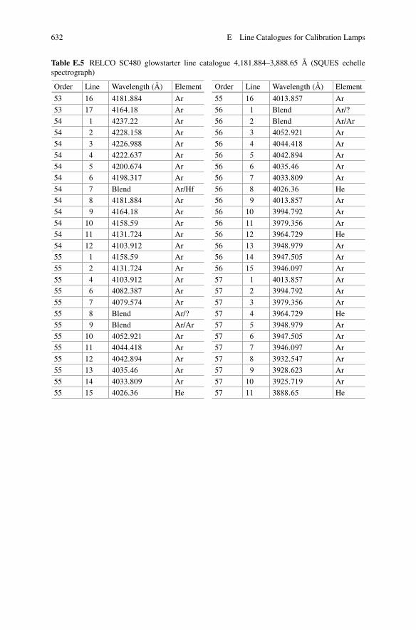
632 E Line Catalogues for Calibration Lamps
Table E.5 RELCO SC480 glowstarter line catalogue 4,181.884–3,888.65 Å (SQUES echellespectrograph)
Order Line Wavelength (Å) Element
53 16 4181:884 Ar
53 17 4164:18 Ar
54 1 4237:22 Ar
54 2 4228:158 Ar
54 3 4226:988 Ar
54 4 4222:637 Ar
54 5 4200:674 Ar
54 6 4198:317 Ar
54 7 Blend Ar/Hf
54 8 4181:884 Ar
54 9 4164:18 Ar
54 10 4158:59 Ar
54 11 4131:724 Ar
54 12 4103:912 Ar
55 1 4158:59 Ar
55 2 4131:724 Ar
55 4 4103:912 Ar
55 6 4082:387 Ar
55 7 4079:574 Ar
55 8 Blend Ar/?
55 9 Blend Ar/Ar
55 10 4052:921 Ar
55 11 4044:418 Ar
55 12 4042:894 Ar
55 13 4035:46 Ar
55 14 4033:809 Ar
55 15 4026:36 He
Order Line Wavelength (Å) Element
55 16 4013:857 Ar
56 1 Blend Ar/?
56 2 Blend Ar/Ar
56 3 4052:921 Ar
56 4 4044:418 Ar
56 5 4042:894 Ar
56 6 4035:46 Ar
56 7 4033:809 Ar
56 8 4026:36 He
56 9 4013:857 Ar
56 10 3994:792 Ar
56 11 3979:356 Ar
56 12 3964:729 He
56 13 3948:979 Ar
56 14 3947:505 Ar
56 15 3946:097 Ar
57 1 4013:857 Ar
57 2 3994:792 Ar
57 3 3979:356 Ar
57 4 3964:729 He
57 5 3948:979 Ar
57 6 3947:505 Ar
57 7 3946:097 Ar
57 8 3932:547 Ar
57 9 3928:623 Ar
57 10 3925:719 Ar
57 11 3888:65 He
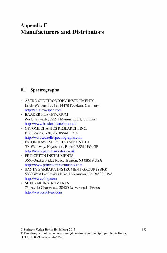
Appendix FManufacturers and Distributors
F.1 Spectrographs
• ASTRO SPECTROSCOPY INSTRUMENTSErich-Weinert-Str. 19, 14478 Potsdam, Germanyhttp://en.astro-spec.com
• BAADER PLANETARIUMZur Sternwarte, 82291 Mammendorf, Germanyhttp://www.baader-planetarium.de
• OPTOMECHANICS RESEARCH, INC.P.O. Box 87, Vail, AZ 85641, USAhttp://www.echellespectrographs.com
• PATON HAWKSLEY EDUCATION LTD59, Wellsway, Keynsham, Bristol BS311PG, GBhttp://www.patonhawksley.co.uk
• PRINCETON INSTRUMENTS3660 Quakerbridge Road, Trenton, NJ 08619 USAhttp://www.princetoninstruments.com
• SANTA BARBARA INSTRUMENT GROUP (SBIG)5880 West Las Positas Blvd, Pleasanton, CA 94588, USAhttp://www.sbig.com
• SHELYAK INSTRUMENTS73, rue de Chartreuse, 38420 Le Versoud - Francehttp://www.shelyak.com
© Springer-Verlag Berlin Heidelberg 2015T. Eversberg, K. Vollmann, Spectroscopic Instrumentation, Springer Praxis Books,DOI 10.1007/978-3-662-44535-8
633
634 F Manufacturers and Distributors
F.2 Fiber Optics
• ASTRO SPECTROSCOPY INSTRUMENTSErich-Weinert-Str. 19, 14478 Potsdam, Germanyhttp://en.astro-spec.com
• CERAMOPTEC Industries Inc.515A Shaker Rd. East Longmeadow, MA 01028, USAhttp://www.ceramoptec.de
• FOP GmbH74564 Crailsheim, Roßfelderstrasse 36, Germanyhttp://www.fop.de
• INSOFT FIBER SHOPSchwarzenberger Str. 41a 51647 Gummersbach, Germanyhttp://www.fiber-shop.de
• LWL SACHSENKABEL GMBHAuerbacher Str. 24, 09390 Gornsdorf, Germanyhttp://www.sachsenkabel.de
• POLYMICRO TECHNOLOGIES18019 N. 25th Avenue, Phoenix, AZ 85023-1200, USAhttp://www.polymicro.com
F.3 Optical Elements: Laboratory Material
• ASTRO SPECTROSCOPY INSTRUMENTSErich-Weinert-Str. 19, 14478 Potsdam, Germanyhttp://en.astro-spec.com/
• BERNHARD HALLE Nachfl. GmbHHubertusstraße 10, 12163 Berlin, Germanyhttp://www.b-halle.de
• CVI MELLES GRIOT200 Dorado Place SE, Albuquerque, NM 87123, USAhttp://www.cvimellesgriot.com
• EDMUND OPTICS Inc.101 East Gloucester Pike, Barrington, NJ 08007-1380 USAhttp://www.edmundoptics.com
• GRATINGWORKS Co.42 Quarry Rd, Acton, MA 01720 USAhttp://www.gratingworks.com
• HORIBA SCIENTIFIC2, Miyanohigashi-cho, Kisshoin, Minami-ku, Kyoto 601-8510, Japanhttp://www.horiba.com
F.3 Optical Elements: Laboratory Material 635
• LASER COMPONENTS GmbHWerner-von-Siemens-Str. 15, 82140 Olching, Germanyhttp://www.lasercomponents.com
• LOT ORIEL GmbH & Co. KGIm Tiefen See 58, 64293 Darmstadt, Germanyhttp://www.lot-oriel.com
• MACONY DESIGNGladiolenstr. 16 16348 Wandlitz, Germanyhttp://www.macony-design.de
• NEWPORT CORPORATION1791 Deere Avenue, Irvine, CA 92606, USAhttp://www.newport.com
• OPTOMETRICS8 Nemco Way, Ayer, MA, 01432, USAhttp://www.optometrics.com
• QIOPTIQ Photonics GmbH & Co. KGKönigsallee 23, 37081 Göttingen, Germanyhttp://www.qioptiq.com
• SCHOTT AGHattenbergstrasse 10, 55122 Mainz, Germanyhttp://www.schott.com
• SHIMADZU, http://www.shimadzu.com/• SILL OPTICS GmbH & Co. KG
Johann-Höllfritsch-Str. 13, 90530 Wendelstein, Germanyhttp://www.silloptics.de
• SPECTRUM SCIENTIFIC, Inc.16692 Hale Avenue, STE A Irvine, CA 92606 USAhttp://ssioptics.com/
• THORLABS56 Sparta Avenue Newton, NJ 07860, USAhttp://www.thorlabs.com
Suggested Reading
• Chrisphin Karthick, M., Astronomer’s Data Reduction Guide: Image processingthrough IRAF commands, LAP LAMBERT Academic Publishing, 2012
A Short Story
Klaus and Thomas regularly discuss questions about spectroscopy and observationsof massive stars with other colleagues. After some time, several questions aboutfundamental optics repeated themselves, especially when novice spectroscopists
636 F Manufacturers and Distributors
wanted to learn something. The same questions popped up again and again andfingers were chopped sore for answers via email and in discussion forums. Thiscould not go on! One day Thomas said “Actually, we should write some explanatorytexts or even a book on the subject, then we can refer to it”. Klaus was not thrilled,thinking of all the work behind it—‘No way!”—and he refused. Thomas then said:“Ok, then I write it alone . . . ”
Bibliography
Abbott, D. C., & Lucy, L. B. (1985). The Astrophysical Journal, 288, 679.Aldoretta, E., et al. (in preparation).Avila, G., Burwitz, V., Guirao, C., Rodriguez, J., Shida, S., & Baade, D. (2007). ESO-Messenger,
No. 129 (p. 62).Avila, G., Burwitz, V., Guirao, C., & Rodriguez, J. (2007). http://www.eso.org/projects/caos/.Avila, G., & Guirao, C. (2009). Tapered optical fibres. http://spectroscopy.wordpress.com.Avila, G., Singh, P., & Chazelas, B. (2010). In SPIE conference proceedings. Ground based and
airborne instrumentation for astronomy III (Vol. 7735, p. 1).Barker, P. K., Landstreet, J. D., Marlborough, J. M., Thompson, I., & Maza, J. (1981). The
Astrophysical Journal, 250, 300.Barker, P. K., Landstreet, J. D., Marlborough, J. M., & Thompson, I. (1985). The Astrophysical
Journal, 288, 741.Bartzakos, P., Moffat, A. F. J., & Niemela, V. S. (2001). Monthly Notices of the Royal Astronomical
Society, 324, 33.Beals, C. S. (1929). Monthly Notices of the Royal Astronomical Society, 90, 202.Beckert, E., et al. (2008). In SPIE conference proceedings. Advanced optical and mechanical
technologies in telescopes and instrumentation (Vol. 7018, p. 82).Behr, A. (1959). Nachr. Akad. Wissenschaften Göttingen 2, Mathem. Physik, K1, 7185.Berek, M. (1970). Grundlagen der praktischen Optik. Walter de Gruyter & Co.Bjorkman, K. S. (1992). In L. Drissen, C. Leitherer, & A. Nota (Eds.), Nonisotropic and variable
outflow from stars. ASP Conference Series (Vol. 22, p. 71).Bjorkmann, J. E., & Cassinelli, J. P. (1993). The Astrophysical Journal, 409, 429.Born, M., & Wolf, E. (1959). Principles of optics. Pergamon PressBouchy, F., Díaz, R. F., Hébrard, G., Arnold, L., Boisse, I., Delfosse, X., et al. (submitted).
Astronomy & AstrophysicsBowen, I. S. (1938) The Astrophysical Journal, 88, 113.Buil, C. (2003). http://www.astrosurf.com/buil/us/compute/simspec.xls.Buil, C. (2006). http://www.astrosurf.com/buil/bestars/m45/img.htm.Buil, C. (2010). http://www.astrosurf.com/buil/star/epsaur/epsaur.htm.Bures, J. (2008). Guided optics: Optical fibers and all-fiber components. Wiley-VCH. ISBN-10:
3527407960.Byard, P. L., & O’Brien, T. P. (2000). In M. Iye & A. F. Moorwood (Eds.), SPIE conference
proceedings. Optical and IR telescope instrumentation and detectors (Vol. 4008, p. 934).Cassinelli, C. P., & Haisch, B. M. (1974). The Astrophysical Journal, 188, 101.
© Springer-Verlag Berlin Heidelberg 2015T. Eversberg, K. Vollmann, Spectroscopic Instrumentation, Springer Praxis Books,DOI 10.1007/978-3-662-44535-8
637
638 Bibliography
Castor, J. I., & Lamers, H. J. G. L. M. (1979). The Astrophysical Journal Supplement Series, 39,481.
Cecil, G., Bland-Hawthorn, J., Veilleux, S., & Filippenko, A. V. (2001). The Astrophysical Journal,555, 338.
Chandrasekhar, S. (1934). Monthly Notices of the Royal Astronomical Society, 94, 522.Chandrasekhar, S. (1946). The Astrophysical Journal, 103, 351.Chandrasekhar, S. (1947). The Astrophysical Journal, 105, 424.Chandrasekhar, S. (1950). The Astronomical Journal, 55, 209.Chini, R., Hoffmeister, V., Kimeswenger, S., Nielbock, M., Nürnberger, D., Schmidtobreick, L.,
et al. (2004). Nature, 429(6988), 155.Chlebowski, T., Harnder, F. R., & Sciortino, S. (1989). The Astrophysical Journal, 341, 427.Clarke, D., & McLean, I. S. (1974). Monthly Notices of the Royal Astronomical Society, 167, 27P.Conti, P. S. (1976). Societé Royale des Sciences de Liége. Mémoires, 9 (p. 193); Discussion (p.
213).Corcoran, M. F., Hamaguchi, K., Pollock, A. M. T., Russell, C. M. P., Moffat, A. F. J., Owocki, S.,
et al. (2012). American Astronomical Society Meeting, 219, 249.Cranmer, S. R., & Owocki, S. P. (1996). The Astrophysical Journal, 462, 469.Crowther, P. A., Smith, L. J., Hillier, D. J., & Schmutz, W. (1995). Astronomy and Astrophysics,
293, 427.Crowther, P. A. (2007). Annual Review of Astronomy & Astrophysics, 45(1), 177.Dougherty, S. M., Beasley, A. J., Claussen, M. J., Zauderer, B. A., & Bolingbroke, N. J. (2005).
The Astrophysical Journal, 623, 447.Drissen, L., St.-Louis, N., Moffat, A.F.J., & Bastien, P. (1987). The Astrophysical Journal, 322,
888.Drissen, L., Robert, C., & Moffat, A. F. J. (1992). The Astrophysical Journal, 386, 288.Ebert, H. (1889). Wied. Ann., 38, 489.Erickson, F. E., & Rabanus, D. (2000). Applied Optics, 39, 4486.Eversberg, T., Lépine, S., & Moffat, A. F. J. (1998). The Astrophysical Journal, 494, 799.Eversberg, T., Moffat, A. F. J., Debruyne, M., Rice, J. B., Piskunov, N., Bastien, P., et al. (1998).
Publications of the Astronomical Society of the Pacific, 110, 1356.Eversberg, T., Moffat, A. F. J., & Marchenko, S. V. (1999). Publications of the Astronomical Society
of the Pacific, 111, 861.Eversberg, T. (2011). Bulletin de la Société Royale des Sciences de Liège, 80, 469.Fabricant, D. G., Hertz, E. H., & Szentgyorgyi, A. H. (1994). In D. L. Crawford & E. R. Craine
(Eds.), SPIE conference proceedings. Instrumentation in astronomy VIII (Vol. 2198, p. 251).Fahed, R., Moffat, A. F. J., Zorec, J., Eversberg, T., Chené, A. N., Alves, F., et al. (2011). Monthly
Notices of the Royal Astronomical Society, 418, 2.Fastie, W. G. (1952). Journal of the Optical Society of America, 42, 647.Federspiel, M. (2002). VdS-Journal, 8, 71.Feger, T. (2012). http://astrospectroscopy.wordpress.com.Feynman, R. P. (1985). QED - The strange theory of light and matter. Princeton, NJ: Princeton
University Press.Gauss, C. F. (1841). Dioptrische Untersuchungen. Göttingen: Verlag der Dieterichschen Buch-
handlung.Gayley, K. G., & Owocki, S. P. (1995) The Astrohysical Journal, 446, 801.Gayley, K. G., Owocki, S. P., & Cranmer, S. R. (1995). The Astrohysical Journal, 442, 296.Gillet, D., et al. (1994). Astronomy & Astrophysics Supplement Series, 108, 181.Gräfener, G., Vink, J. S., de Koter, A., & Langer, N. (2011) Astronomy & Astrophysics, 535, 56.Gray, F. D. (1992). The observation and analysis of stellar photospheres. Cambridge Astrophysics
Series 20.Green, J. C., Froning, C. S., Osterman, S., Ebbets, D., Heap, S. H., Leitherer, C., et al. (2012). The
Astrohysical Journal, 744, 60.Grosdidier, Y., Moffat, A. F. J., Blais-Ouellette, S., Joncas, G., & Acker, A. (2001). The
Astrophysical Journal, 562, 753.
Bibliography 639
Gross, H., Zügge, H., Peschka, M., & Blechinger, F. (2007). Handbook of Optical Systems,Aberration Theory and Correction of Optical Systems, Wiley-VCH, (Vol. 3).
Grupp, F. (2003). Astronomy & Astrophysics, 412, 897.Guinouard, I., et al. (2006) In E. Atad-Ettedgui, J. Antebi, & D. Lemke (Eds.), SPIE conference
proceedings. Optomechanical technologies for astronomy (Vol. 6273, p. 3).Hall, J. S. (1949). Science, 109, 165.Hamann, W.-R., Gräfener, G., & Liermann, A. (2006). Astronomy & Astrophysics, 457, 1015.Hamann, W. R. (2011). Private communication.Harries, T. J. (1995). Spectropolarimetry as a probe of stellar winds. Ph.D. thesis. University
College London.Harries, T. J., & Howarth, I. D. (1996). Astronomy & Astrophysics, 310, 553.Hartwig, G., & Schopper, H. (1959). Bulletin of the American Physical Society, 4, 77.Hayes, D. P. (1984). Astronomical Journal, 89, 1219.Haynes, D. M, Withford, M. J., Dawes, J. M., Haynes, R., & Bland-Hawthorn, J. (2008). In E. Atad-
Ettedgui & D. Lemke (Eds.), SPIE conference proceedings. Advanced optical and mechanicaltechnologies in telescopes and instrumentation (Vol. 7018, p. 8).
Heathcote, B. (2013). Private communication.Hecht, E., & Zajac, A. (2003). Optics (4th ed.).Hill, G. M., Moffat, A. F. J., St-Louis, N., & Bartzakos, P. (2000) Monthly Notices of the Royal
Astronomical Society, 318, 402.Hillier, D. J., Kudritzki, R.-P., Pauldrach, A. W. A., Baade, D., Cassinelli, J. P., Puls, J., et al.
(1993). Astronomy & Astrophysics, 276, 128.Hiltner, W. A. (1949). Science, 109, 165.Hutley, M. C. (1982). Diffraction Gratings, Techniques of Physics (Vol. 6). Academic Press.Huwiler, M. www.eagleowloptics.com.James, J. F. (2007). Spectrograph design fundamentals. New York: Cambridge University Press.Jiang, Y. M., Walker, G. A. H., Dinshaw, N., & Matthews, J. M. (1993). In L. A. Balona, H. F.
Henrichs, & J. M. Le Contel (Eds.), Pulsation, rotation and mass loss in early-type stars. Proc.IAU Symp. No. 163 (p. 232). Dordrecht: Kluwer.
Kaper, L., Henrichs, H. F., Fullerton, A. W., Ando, H., Bjorkman, K. S., Gies, D. R., et al. (1997).The Astrohysical Journal, 327, 281.
Kataza, H., Okamoto, Y., Takubo, S., Onaka, T., Sako, S., Nakamura, K., et al. (2000).InM. Iye & A. F. Moorwood (Eds.), SPIE conference proceedings. Optical and IR telescopeinstrumentation and detectors (Vol. 4008, p. 1144).
Kaufer, A., & Pasquini, L. (1998). In S. D’Odorico (Ed.), SPIE conference proceedings. Opticalastronomical instrumentation (Vol. 3355, p. 844).
Kaufer, A. (1998). ASP Conference Series (Vol. 152, p, 337).Kay, L., & Shepherd, R. (1982). Journal of Physics E: Scientific Instruments, 16.Kayser, H. (1900). Handbuch der Spectroscope, 1.Kenworthy, M. A., Parry, I. R., & Taylor, K. (2001). Publications of the Astronomical Society of
the Pacific, 113, 215.Keyes, C. D., Long, K., & Hunter, D. (2006). STScI JWST Configuration Management - JWST-
STScI-000851, SM-12.Kodak Application Note MTD/PS-0233. (2003). CCD image sensor noise sources. Eastman Kodak
CompanyKotelnikov, V. A. (1933, January 14). O propusknoj sposobnosti ’efira’ i provoloki v elektrosvjazi,
(On the transmission capacity of ’ether’ and wire in electro-communication). Proceedings ofthe first all-union conference on the technological reconstruction of the communications sectorand the development of low-current engineering. Moscow.
Krane, K. S. (1988). Introductory nuclear physics (p. 537). New York: John Wiley & Sons.Kroupa, P. (2000, March 20–24). Astronomische Gesellschaft meeting abstracts. Heidelberg. Talk
no. 11.Lamers, H. J. G. L. M., Zickgraf, F.-J., de Winter, D., Houziaux, L., & Zorec, J. (1998). Astronomy
& Astrophysics, 340, 117.
640 Bibliography
Lamers, H. J. G. L. M., & Cassinelli, J. P. (1999). Introduction to stellar winds. CambridgeUniversity Press
Landstreet, J. D. (1979). The Astronomical Journal, 85, 611.Langer, N., Hamann, W.-R., Lennon, M., Najarro, F. Pauldrach, A. W. A., & Puls, J. (1994).
Astronomy and Astrophysics, 290, 819.Leadbeater, R. (2010). http://www.threehillsobservatory.co.uk.Leadbeater, R. (2011). In T. Eversberg & J. H. Knapen (Eds.), Stellar winds in interaction,
arXiv:1101.1435.Leadbeater, R., Buil, C., Garrel, T., Gorodenski, S., Hansen, T., Schanne, L. et al. (2012).
arXiv:1206.6754.Lépine, S., Eversberg, T., & Moffat, A. F. J. (1999). The Astronomical Journal, 117, 1441.Lépine, S., & Moffat, A. F. J. (1999). The Astronomical Journal, 514, 909.Lépine, S., & Moffat, A. F. J. (2008). The Astronomical Journal, 136, 548.Lesh, J. R. (1968). The Astrophysical Journal Supplement Series, 17, 371.Lo Curto, G. (2012). ESO Messenger No. 149 (p. 2).Lührs, S. (1997). Publications of the Astronomical Society of the Pacific, 109, 504.Lupie, O. L., & Nordsieck, K. H. (1987). Astronomical Journal, 92, 214.Maeder, A. (1999). Astronomy & Astrophysics, 347, 185.Marchenko, S. V., et al. (2001). The Astrophysical Journal, 596, 1295.Marchenko, S. V., Moffat, A. F. J., Vacca, W. D., Côté, S., & Doyon, R. (2002). The Astrophysical
Journal, 565, 59.Marchenko, S. V., Moffat, A. F. J., Ballereau, D., Chauville, J., Zorec, J., Hill, G. M., et al. (2003).
The Astrophysical Journal, 596, 1295.Massey, P., & Hanson, M. M. (2010). arXiv:1010.5270.Mauclaire, B., Buil, C., Garrel, T., & Lopez, A. (2013). arXiv:1207.0795.McLean, I. S. (1978). Monthly Notices of the Royal Astronomical Society, 186.McLean, I. S., Coyne, G.V., Frecker, J.E., Serkowski, K., 1979, The Astrophysical Journal, 228,
802.McLean, I. S., Coyne, G. V., Frecker, J. E., Serkowski, K. (1979). The Astrophysical Journal, 231,
L141.McComas, D. J., Bame, S. J., Barraclough, B. L., Feldman, W. C., Funsten, H. O., Gosling, J. T.,
et al. (1998). Geophysical Research Letters, 25(1), 1.Menn, N. (2004). Practical optics. Academic Press.Meynet, G., Georgy, C., Hirschi, R., Maeder, A., Massey, P., Przybilla, N., et al. (2011). In G.
Rauw, M. De Becker, Y. Nazé, J.-M. Vreux, & P. Williams (Eds.), Proceedings of the 39thLiège Astrophysical Colloquium (Vol. 80, p. 266).
Mihalas, D. (1970). Stellar atmospheres. San Francisco: W. H. Freeman and Co.Miroshnichenko, A.S., Pasechnik, A.V., Manset, N., Carciofi, A.C., Rivinius, Th., Stefl, S., et al.
(2013). The Astrophysical Journal, 766, 119.Moffat, A. F. J. (1969). Astronomy & Astrophysics, 3, 455.Moffat, A. F. J., & Robert, C. (1994). The Astrophysical Journal, 421, 310.Morel, T., Alves, F., Bergmann, T., Carrera, L. F. G., Dias, F. M., Eversberg, T., et al. (submitted).
Astronomy and Astrophysics.Morel, T., Rauw, G., Eversberg, T., Alves, F., Arnold, W., Bergmann, T., et al. (2011). G. Rauw,
M. De Becker, Y. Nazé, J.-M. Vreux, & P. Williams (Eds.), Proceedings of the 39th LiègeAstrophysical Colloquium (Vol. 80. p. 170).
Morel, T., St.-Louis, N., & Marchenko, S. (sumbitted). The Astrophysical Journal.Moore, B. D., Hester, J. J., & Scowen, P. A. (2000). The Astronomical Journal, 119, 2991.Moore, B. D., Walter, D. K., Hester, J. J., Scowen, P. A., Dufour, R. J., & Buckalew, B. A. (2002).
The Astronomical Journal, 124, 3313.Motz, H., Thon, W., & Whitehurst, R. N. (1953). Journal for Applied Physics, 24, 826.Naze, Y., Rauw, G., Herve, A., & Oskinova, L. (2011, June 27–30). In The X-ray universe 2011,
Conference held in Berlin, Germany. Article id.111.
Bibliography 641
Newberry, M. (1998–2000). Measuring the gain of a CCD camera (Axiom Tech Note 1). AxiomResearch Inc.
Nemravová, J., Harmanec, P., Koubský, P., Miroshnichenko, A., Yang, S., Slechta, M., et al. (2012).Astronomy & Astrophysics, 537, 11.
Noguchi, K., Aoki, W., Kawanomoto, S., Ando, H., Honda, S., Izumiura, H., et al. (2002).Publications of the Astronomical Society of Japan, 54, 855.
Nordsieck, K. H., Babler, B., Bjorkman, K. S., Meade, M. R., Schulte-Ladbeck, R. E., Taylor, M.J. (1992). In L. Drissen, C. Leitherer, & A. Nota (Eds.), Nonisotropic and variable outfow fromstars. ASP Conference Series (Vol. 22, p. 114).
Nyquist, H. (1928). Transactions of the American Institute of Electrical Engineers, 47, 617.Okazaki, A. T. (1991). Publications of the Astronomical Society of Japan, 43, 75.O’Shea, D. C. (1985). Elements of modern optical design. Wiley Series in Pure and Applied Optics.Osmer, P. S., et al. (2000). In M. Iye & A. F. Moorwood (Eds.), SPIE conference proceedings.
Optical and IR telescope instrumentation and detectors (Vol. 4008, p. 40).Owocki, S. P. (1996). Quebec – Delaware annual meeting on massive stars. Private communicationOwocki, S. P. (1998). Turbulence in line-driven stellar winds. Workshop on ‘Interstellar Turbu-
lence’ held January 1998 in Puebla, Mexico.Owocki, S. P. (2004). In M. Heydari-Malayeri, Ph. Stee, & J.-P. Zahn (Eds.), Evolution of Massive
Stars. EAS Publications Series (Vol. 13, p. 163).Owocki, S. P., Gayley, K. G., & Shavic, N. J. (2004). The Astrophysical Journal, 616, 525.Owocki, S. P. (2013). Private communication.Picht, J. (1955). Grundlagen der geometrisch-optischen Abbildung. Berlin: VEB Deutscher Verlag
der Wissenschaften.Pierce, A. K. (1965). Publications of the Astronomical Society of the Pacific, 77, 216.Poeckert, R., Marlborough, J. M. (1977). The Astrophysical Journal, 218, 220.Poeckert, R., & Marlborough, J. M. (1978). The Astrophysical Journal, 220, 940.Pogge, R. W., et al. (2006). In I. S. McLean, & Iye, M. (Eds.), SPIE conference proceedings.
Ground-based and airborne instrumentation for astronomy (Vol. 6269, p. 62690I).Pogge, R. W., et al. (2010). In I. S. McLean, S. K. Ramsay, & Takami, H. (Eds.), SPIE conference
proceedings. Ground-based and airborne instrumentation for astronomy III (Vol. 7735, p.77350A).
Puls, J., Kudritzki1, R.-P., Herrero, A., Pauldrach, A. W. A., Haser, S.M., Lennon, D. J., et al.(1996). Astronomy & Astrophysics, 305, 171.
Pyo, T.-S. (2003). IRCS echelle spectrograph and data handling. Subaru Telescope NationalAstronomical Observatory.
Prinja, R. K., & Howarth, I. D. (1986). The Astrophysical Journal Supplement Series, 61, 357.Ramsey, L. W. (1988) In S. C. Barden (Ed.), Fibers optics in astronomy. ASP Conf. Ser. 3, Tucson
(p. 26).Rauw, G., Alves, F., Bergmann, T., Carrera, L. F. G., Dias, F. M., Eversberg, T., et al. (submitted).
Astronomy and Astrophysics.Reiner, J. (2002). Grundlagen der Ophthalmologischen Optik, Books on Demand.Reipurth, B., Yu, K. C., Rodríguez, L. F., Heathcote, S., & Bally, J. (1999). Astronomy and
Astrophysics, 352, L83.Richardson, N., et al. (in preparation).Robb, P. N. (1985). Applied Optics, 24, 1864.Robert, C., & Moffat, A. F. J. (1989). The Astrophysical Journal, 343, 902.Robert, C., Moffat, A. F. J., Bastien, P., Drissen, L., & St-Louis, N. (1989). The Astrophysical
Journal, 347, 1034.Robert, C., Moffat, A. F. J., Bastien, P., St-Louis, N., & Drissen, L. (1990). The Astrophysical
Journal, 359, 211.Robert, C., Moffat, A. F. J., Drissen, L., Lamontagne, R., Seggewiss, W., Niemela, V. S., et al.
(1992). The Astrophysical Journal, 397, 277.Robert, C. (1992). Dissertation Abstracts International (Vol. 55-03, Section B, p. 0953). PhD
thesis, Université de Montréal (Canada).
642 Bibliography
Robinson, L. B. (1988). Instrumentation for ground-based optical astronomy. Springer.Rosenhauer, K., & Rosenbruch, K. J. (1960). Optik, 17, 249–277.Ruždjak, et al. (2009). Astronomy & Astrophysics, 506, 1319.Sablowski, D. (2012). In Spektrum - Mitteilungsblatt der Fachgruppe Spektroskopie in der
Vereinigung der Sternfreunde e.V., No. 43. http://spektroskopie.fg-vds.de/pdf/Spektrum43.pdf.Sahnow, D. J., Friedman, S. D., Oegerle, W. R., Moos, H. W., Green, J. C., & Siegmund, O. H.
(1996). In SPIE conference proceedings. Space telescopes and instruments IV (Vol. 2807, p. 2).Sander, A., Hamann, W.-R., & Todt, H. (2012). Astronomy & Astrophysics, 540, A144.Schaerer, D., Schmutz, W., & Grenon, M. (1997). The Astrophysical Journal, 484, L153.Schroeder, D. J. (1967). Publications of the Astronomical Society of the Pacific, 82, 1253.Schroeder, D. J. (1970). Applied Optics, 6(11).Schroeder, D. J. (1987). Astronomical Optics, Academic Press.Schulte-Ladbeck, R. E., Nordsieck, K. H., Nook, M. A., Magalhães, A. M., Taylor, M., Bjorkman,
K. S., et al. (1990). The Astrophysical Journal, 365, L19.Schulte-Ladbeck, R. E., Nordsieck, K. H., Taylor, M., Nook, M. A., Bjorkman, K. S., Magalhães,
A. M., et al. (1991). The Astrophysical Journal, 382, 301.Schulte-Ladbeck, R. E., Meade, M., & Hillier, D. J. (1992). In L. Drissen, C. Leitherer, & A. Nota
(Eds.), Nonisotropic and variable outflow from stars. ASP Conference Series (Vol. 22, p. 118).Schulte-Ladbeck, R. E., Nordsieck, K. H., Taylor, M., Bjorkman, K. S., Magalhães, M. A., &
Wolff, M. J. (1992a). The Astrophysical Journal, 387, 347.Schulte-Ladbeck, R. E., Nordsieck, K. H., Code, A. D., Anderson, C. M., Babler, B.L., Bjorkman,
K. S., et al. (1992b). The Astrophysical Journal, 391, L37.Schulte-Ladbeck, R. E., Eenens, P. R., & Davis, K. (1995). The Astrophysical Journal, 454, 917.Schwarzschild, M. (1950). The Astrophysical Journal, 112, 222.Seidel, L. (1856). Astronomische Nachrichten, 43, 289.Semel, M. (1989). Astronomy & Astrophysics, 225, 456.Serkowski, K. (1962). Advances in Astronomy and Astrophysics, 1, 247.Serkowski, K. (1970). The Astrophysical Journal, 160, 1083.Serkowski, K. (1974). Methods of Experimental Physics, 12 (Chap. 8).Serkowski, K., Mathewson, D. S., & Ford, V. L. (1975). The Astrophysical Journal, 196, 261.Serkowski, K., Mathewson, D. S., & Ford, V. L. (1975). The Astrophysical Journal, 196, 261.Shafer, A. B., et.al. (1964). Journal of the Optical Society of America, 54, 7.Shannon, C. E. (1948). Bell System Technical Journal, 27, 379.Shannon, C. E. (1948). Bell System Technical Journal, 27, 623.Sharma, A. B., Halme, S. J., & Butusow, M. M. (1981). Optical fibre systems and their components.
Springer.Shurcliff, W. (1962). Polarized light. Cambridge University Press.Silva, D. R., & Cornell, M. E. (1992). The Astrophysical Journal Supplement Series, 81, 865.Sletteback, A. (1979). Space Science Review, 23, 541.Slijkhuis, S. (2012). In Spektrum - Mitteilungsblatt der Fachgruppe Spektroskopie in der Vereini-
gung der Sternfreunde e.V., No. 43. http://spektroskopie.fg-vds.de/pdf/Spektrum43.pdf.Smith, S. J., & Purcell, E. M. (1953). Physical Review, 92, 1069.Smith, M. A., Robinson, R. D., & Corbet, R. H. D. (1998). The Astrophysical Journal, 503, 877.Smith, M. A., Robinson, R. D., & Hatzes, A. P. (1998). The Astrophysical Journal, 507, 945.Smith, M. A., & Robinson, R. D. (1999). The Astrophysical Journal, 517, 866.St-Louis, N., Drissen, L., Moffat, A. F. J., Bastien, P., & Tapia, S. (1987). The Astrophysical
Journal, 322, 870.St-Louis, N., Moffat, A. F. J., Drissen, L., Bastien, P., & Robert, C. (1988). The Astrophysical
Journal, 330, 286.St-Louis, N., Moffat, A. F. J., Lapointe, L., Efimov, Yu. S., Shakhovskoy, N.M., Fox, G. K., et al.
(1993). The Astrophysical Journal, 410, 342.St-Louis, N., Dalton, M. J., Marchenko, S. V., Moffat, A. F. J., & Willis, A. J. (1995). The
Astrophysical Journal, 452, 57.St-Louis, N., Doyon, R., Chagnon, F., & Nadeau, D. (1998). The Astronomical Journal, 115, 2475.
Bibliography 643
Stee, Ph., Vakili, F., Bonneau, D., & Mourard, D. (1998). Astronomy & Astrophysics, 332, 268.Sundqvist, J. O., Owocki, S. P., & Puls, J. (2012). In ASP Conference Series (Vol. 465, p. 119).Suto, H., & Takami, H. (1997). Applied Optics, 38(19).Taubert, R. D., Monte, C., Baltruschat, C., Schirmacher, A., Gutschwager, B., Hartmann, J., et al.
(2009). Metrologia, 46(4), 207.Taylor, M. (1992). In L. Drissen, C. Leitherer, & A. Nota (Eds.), Nonisotropic and variable outflow
from stars. ASP Conference Series (Vol. 22, p. 57).Telting, J, H., & Kaper, L. (1994). Astronomy and Astrophysics, 284, 515.Thizy, O. (2007). In Proceedings of the 26th annual symposium on telescope science, Society for
Astronomical Sciences (p. 31).Tüg, H. (1974). Astronomy and Astrophysics, 37, 249.Tüg, H. (1980). Astronomy and Astrophysics, 82, 195.Tüg, H., White, N. M., & Lockwood, G. W. (1977a). Astronomy and Astrophysics, 61, 679.Tüg, H., White, N. M., & Lockwood, G. W. (1977b). Astronomy and Astrophysics, 66, 469.Vernet, J., et al. (2011). Astronomy and Astrophysics, 536, 105.Vollmann, K., & Eversberg, T. (2006). Astronomical Notes, 327, 862.Vollmann, K. (2008). http://www.stsci.de/simspec$_$slit$_$e.xls.Walder, R., & Folini, D. (2002). In Proc. IAU Symposium No. 212.Waldschläger, U. (2014). Private communication.Walraven, T., & Walraven, J. H. (1972). In S. Lausten & A. Reiz (Eds.), Proceedings of the
Conference on Auxiliary Instrumentation for Large Telescopes (p. 175).Whittaker, E. T. (1915). Procceedings of the Royal Society Edinburgh, 35, 181.Whittaker, J. M. (1935). Interpolatory function theory. Cambridge University Press.Widenhorn, R., Blouke, M. M., Weber, A., Rest, A., & Bodegom, E. (2002). In SPIE conference
proceedings. Sensors and camera systems for scientific, industrial, and digital photography(Vol. 4669).
Wilken, T., Lo Curto, G., Probst, R. A., Steinmetz, T., Manescau, A., Pasquini, L., et al. (2012).Nature, 485, 611.
Witt, V. (2005). Sterne und Weltraum, 10, 73.Wood, K., Brown, J. C., & Fox, G. K. (1993). Astronomy and Astrophysics, 271, 492.v. Zeipel, H. (1924). Monthly Notices of the Royal Astronomical Society, 84, 702.
Index
˛ Eridani, 493ı-function (Dirac), 38� Aurigae, 334, 555� Velorum, 481� configuration (echelle), 199�/2 retarder, 542�/4 retarders, 542p
n rule, 470‚ configuration (echelle), 199� Puppis, 481� Tauri, 466
Abbe invariant of paraxial rays, 88Abbe number, 102Aberration, 95Absolute measurements, 453Absorption, 481Acceptance cone, 417Achernar, 493Achromat, 239Achromatic lens, 263Air grooves, 378Airy disk, 27, 158, 239Alignment, 283Amplification factor, 399Amplifier, 395
noise, 389Analog-to-digital (AD) converter, 387, 388,
395Analog-to-digital unit (ADU), 387Anamorphic magnification factor, 54, 170,
176, 214, 232Angle of incidence, 193, 201
grating, 10, 13
Angle of refraction, 255Angular dispersion, 31, 165, 201Aperture aberration, 96Apochromat, 104ARAS, 556Argon, 163
calibration lamp, 460Arithmetic mean, 468Artificial fitting function, 447Artificial vignetting, 188Aspheric surfaces, 135Astigmatism, 86, 96, 116, 119, 264Atmospheric turbulence, 28Atomic clocks, 462Atomic ionization stages, 496Attenuation, 418Average error of the function value, 470Average image curvature, 119Average opacity, 485Axisymmetric clumps, 548
Baby lamp, 328Background noise, 408Background subtraction, 448Baffle, 162, 275Baffling, 135Band gap (CCD), 392Be star disks, 487Be stars, 487, 493, 496, 531Beam deflection, 13Beam-splitting analyzers, 537Beam width, 165Bending behaviour, 411BESO (spectrograph), 356
© Springer-Verlag Berlin Heidelberg 2015T. Eversberg, K. Vollmann, Spectroscopic Instrumentation, Springer Praxis Books,DOI 10.1007/978-3-662-44535-8
645
646 Index
Bessel function, 26, 27, 65, 158, 591Best focus, 265Best form lens, 140Beta value, 487Bias, 390Bias field, 441, 443Binning, 177
mode, 391Blaze angle, 46, 197, 212, 223Blaze efficiency (maximum), 221Blaze function, 42Blaze surface, 223Blaze wavelength, 46Blooming, 388Blueshifted atomic lines, 483Blurring area, 235Blurring circle, 124, 126, 127, 238, 265Boller & Chivens, 337Boller & Chivens (spectrograph), 322Boltzmann distribution, 392Bowen slicer, 371Bowen–Walraven slicer, 374Bremsstrahlung, 530, 548Brewster angle, 375Broadening processes, 67Bubble nebula, 525Bunsen, Robert, 4
Calibration, 162assembly, 451
Camera, 54, 165, 242mirror, 283tilt, 267
Campaigns, 555CAOS (group), 383CAOS low cost image slicer, 383Cardinal series, 73CASPEC (polarimeter), 538Central limit theorem, 68Central wavelength (echelle), 201Central wavelength spacing, 234Cerenkov effect, 530Charge Coupled Device (CCD), 387
gain, 400, 442reduction, 441
Chief ray, 140Chromatic aberration, 86, 231, 239, 264Circle of confusion, 121, 291Circle of least confusion, 98, 292Circularly polarized light, 531Cladding, 412Clumps, 513Co-rotating interaction regions, 2, 499
Collapsing the spectrum, 448Collimator, 30, 54, 164, 235
mirror, 283Collision shocks, 496Colour temperatures, 449Coma, 86, 96, 264COMICS (spectrograph), 345Concave mirrors, 281, 284Conduction band, 392Cone-tip, 518Conic parameterization, 287Constructive interferences, 37Contexts (MIDAS), 562Conti scenario, 517Continuous Fourier transform, 600Continuum-forming region, 546Continuum noise, 467Conversion factor, 400Cooke triplet, 148Coriolis force, 520Corona, 435COS (spectrograph), 366Cosmic rays, 458Critical angle, 420Cross-disperser, 229, 253
echelle, 197, 211Cross-talk, 211, 233Cryostat, 345, 393Cubic splines, 596Curve-of-growth method, 480Curved orders, 209Cycloid, 184Cyclotron emission, 548Cyclotron radiation, 530Czerny-Turner (spectrograph), 334
DADOS (spectrograph), 323Damping constant, 418Dark current, 392Dark field, 441, 443Dark noise, 392Data reduction, 439
echelle, 276MIDAS, 561recipe, 454
Dead pixels, 402Definition phase, 322Deflection, 411
angle, 255Degree of ellipticity, 533Degree of polarization, 533Deneb, 158Depth of focus, 126, 127, 235, 244
Index 647
Descartes (René), 9Destructive interferences, 37Detection threshold, 405Detector noise, 407Diaphragm systems, 99Dichroic filter, 342Diffraction angle, 193
difference, 201Diffraction effects, 173Diffraction factor, 208, 213, 219Diffraction grating, 36Diffraction index, 10Diffraction indices of various glasses, 601Diffraction law, 9Diffraction pattern, 27Diffuse concentric rings, 447Dilution effect, 547Discrete absorption components, 499Disk temperature, 491Dispersion, 469
element, 166relation, 31
Distortion, 99, 117Distributors, 633Doppler effect, 483Double calcite plate, 537Double Rochon prism, 537Drift, 467Dust particles, 447Dynamics (CCD), 388
Early-type stars, 544Ebert-Fasti spectrograph, 282Echelle spectrograph, 196Echelle spectroscopy, 197Eddington luminosity, 485Effective blaze area, 224Effective etendue, 224Effective gravitational acceleration, 494Electric vector, 533Electron scattering, 482Electron-scattering region, 546Elliptical polarized light, 533Emission line stars, 478Emulator, 441Envelope shape factor, 545Equivalent width of spectral lines, 472Error of the equivalent width, 474EShel (spectrograph), 353EShel guiding unit, 354ESPaDOnS (polarimeter), 538Etendue, 216, 429
conservation, 217
Evolution, 517Exoplanets, 334Expectance value (Poisson), 593Exposure time, 442
estimation, 459Extraordinary beam, 537, 539EZ CMa, 546
F-number change, 412F-number conservation, 217Faceplate, 162Facets, 200
shadowing, 224Far-field approximation, 43Feasibility study, 322Feger echelle (spectrograph), 350Femtosecond pulsed laser, 463Fermat, 10FEROS (spectrograph), 356FEROS fiber link, 432FEROS image slicer, 377Fiber bundle, 331Fiber loss, 418Fiber noise, 423Fiber optics, 411
contributors, 634Fiber speckles, 425Fiber-stress, 411Fiber types, 412Field angle, 259Field curvature, 86, 99, 118, 231, 264Field error, 265Field flattener, 142, 3325th order Legendre function, 447Final instrument, 322Finite support, 75, 77Fits format, 562Fitting package (MIDAS), 562Fixed pattern noise (CCD), 402Flat field, 441, 445Flat line profiles, 506Flats for echelle spectroscopy, 448Flexure, 411Focal length, 91Focal-ratio degradation (FRD), 171, 413, 419,
542Foci, 94Folding integral, 63Footprints (image slicer), 374Fourier correspondences, 600Fourier transform, 22, 25
2-dimensional, 25N-dimensional, 22
648 Index
Fraunhofer diffraction, 19, 38, 235Fraunhofer equation, 16Fraunhofer, Joseph, 4Free electrons, 387Free-free transitions, 482Free spectral range, 202, 203, 233Fresnel, 10, 18
diffraction, 22equations, 10, 594
Fresnel–Kirchhoff diffraction integral, 22, 41Full width at half maximum (FWHM), 45, 63,
66, 123, 161, 173Full-well capacity, 388Fundamental theorem of calculus, 473FUSE (spectrograph), 363
Gain (CCD), 389Gamma function, 591Garrison spectrograph, 322Gauss error propagation, 471Gaussian image, 105
plane, 88Gaussian lens equation, 93Gaussian normal distribution, 468Gaussian plane, 291General angular dispersion, 198Geometrical order length, 200Glan-Foucault prism, 537Glan-Taylor prism, 540Glan-Thompson prism, 537Glow starter, 163
RELCO SC480, 618Gradient index fibers, 413Grating (cross-disperser), 253Grating constant, 197, 221Grating equation, 37, 193, 197
in a general form, 194Grating facets, 47, 223Grating function, 40Grating interference function, 250Grating plus electron beam, 530Gravity darkening, 494Gray level, 387Grey-body magneto-emission, 531Groove density, 203Guiding unit, 354Gyro-resonance emission, 531
Half-Wave Polarimeter, 538Halogen lamps, 449Hanle effect, 531HARPS (spectrograph), 462
HD 93129, 503HD 164794, 480HD 192163, 506HD 192793, 507HD 59468, 480HDS (spectrograph), 358Hectoechelle (spectrograph), 339Hectospec (spectrograph), 339Heisenberg uncertainty principle, 70Helium, 163
calibration lamp, 460Helium-argon, 163Hertzsprung-Russell diagram, 480HgCdTe detector, 362High orders, 197Hollow-cathode lamps, 163Hooker Telescope, 5Hot pixels, 402Hot stars, 480H� transitions, 482Humidity fluctuations, 412Huygens (Cristiaan), 18Huygens principle, 18Huygens–Fresnel principle, 17Hydrodynamic simulation of DACs, 501Hydrostatic equilibrium, 485Hydrostatic stellar surface, 483
Image and graphic display (MIDAS), 562Image slicer, 369Imaging equation, 285Incandescent lamps, 449Incidence height, 87Index of diffraction, 10Index of refraction, 32Initial Mass Function, 525Integral field spectroscopy, 331, 412Integral-field unit, 378Integral nonlinearity, 390Integrating spheres, 449Interference function, 40Interference patterns, 19Interference phenomena, 17Interferometric measurements, 496Intermediate focus, 275Intermediate optics, 431International Ultraviolet Explorer, 493Intersection length, 86Interstellar polarization, 543Intrinsic circular polarization, 548Intrinsic fiber noise, 412Intrinsic linear polarization, 544Inverse linear dispersion, 52, 255
Index 649
IRAF, 440echelle data reduction, 276
IR spectroscopy, 345Iron, 163
calibration lamp, 460forest, 510
Iso-wavelength contours, 483
James Webb Telescope, 451
K-capture of high-energy gamma-rays, 530Küpfmüller uncertainty principle, 70Kepler telescope, 145Kirchhoff (Gustav Robert), 4, 18Knife-edge method, 327
Lührs model, 520Laboratory material (contributors), 634Lambert cosine law, 449Lambert surfaces, 449Laser frequency combs, 461Last scattering surface, 507Late-type stars, 453Law of diffraction, 9Law of large numbers, 443LBT (telescope), 342Lens bending, 136Lens distances, 137Lensmaker equation, 91Lens splitting, 137Lhires III (spectrograph), 323, 328Light flux, 442Light from canal rays, 530Limiting magnitude, 172Line broadening, 479Line catalogue sources, 617Line catalogues for calibration lamps, 617Line density, 245Line-emitting region, 546Line-profile analysis, 440Line scattering, 482Linear dispersion, 31, 254Linear polarization, 531Linear response, 389Lines of equal radial velocity, 483LINUX, 440Littrow configuration, 50Littrow spectrograph, 170Littrow systems, 324Longitudinal aberration, 95
Longitudinal chromatic aberration, 100, 239,267
curve, 104Longitudinal field, 549Longitudinal spherical aberration, 286Long-term observations, 553Low-order fitting function, 447Luminous Blue Variables, 511, 517
M1-67 (nebula), 510Magnetic fields, 529, 549Magnetic flares, 496Magnetic spots, 552Magnification factor, 181Mahlmann Littrow (spectrograph), 326Main sequence, 506Management, 322Manufacturers, 633Mars (planet), 6Massive stars, 477, 480Mass-luminosity relation, 480Master bias, 443Master dark, 444Master flat, 446Matrix method, 93Maximum beam diameter, 176Maximum resolving power, 35MCL Debugger (MIDAS), 562Mean error of single measurements, 469Mean field curvature, 116Measurement errors, 465Median filtering, 458Meridional incident light, 414Meridional field curvature, 115Meridional plane, 414Meridional rays, 414MESSY (spectrograph), 170Metallicity, 478Mice Mansion (spectrograph), 333Micro-bending, 420Micro-lenses, 434MIDAS, 440
data reduction, 561echelle data reduction, 276
MIDAS Control Language, 562Mini-Echelle, 258Mirror collimator, 230Mirror spectrometer, 284Mizar, 334MMT (telescope), 339Modes, 412MODS (spectrograph), 342Moffat function, 160
650 Index
Momentum problem, 509Monitoring, 554Monochromatic (order), 243Monochromatic Seidel aberrations, 94Monochromator, 282Mono-mode fibers, 414Mount Wilson, 5Mueller calculus, 534Mueller matrix, 535Multimode fibers, 412Multi-object double spectrograph, 342Multi-object spectroscopy, 339Multiple convolution, 67Multiple scattering in the wind, 509
Natural aperture, 139Natural vignetting, 188Necessary flat field quality, 456Neon, 163
lamps, 459Newtonian rings, 17NGC 2359, 526NGC 3079, 527NGC 7635, 525Nicol prism, 536Nodal points, 94Noise (CCD), 391Noise contribution (bias & dark), 455Non-spherical grains, 543Normal dispersion, 103Normal glasses, 103Normalized master flat, 446Numerical aperture, 129, 418Nyquist criterion, 72Nyquist–Shannon theorem, 72, 176
Object distance, 181OB stars, 499Off-axis aberration, 231Off-axis angle, 194, 204Off-axis configuration, 281Off-axis mode, 282Offset signal, 390One-armed disk, 492One-dimensional Fourier transform, 600OCO binaries, 518Opacity, 488
problem, 510Open source, 439Optical density, 489Optical elements (contributors), 634Optical slit, 158
Optically thick lines, 491Optically thick wind, 483Optically thin lines, 489Optically thin material, 488Optically thin shell, 506Optics of a prism, 10Opto-mechanical coupling, 435Order cross-section, 274Order normal, 204Order number, 194
echelle, 201Order separation, 233Ordinary beam, 536, 539O stars, 487Outward moving stellar wind, 483Overflow, 388Overlapping orders, 197Oversampling, 82, 83, 177
Parabolic mirrors, 281Parameter fluctuations, 453Paraxial approximation, 285Paraxial chromatic aberration, 268Paraxial image scale, 89Paraxial light beam, 87Partial coefficients, 110, 111Path difference, 194, 200P Cygni, 481Peltier element, 393PEPSI (spectrograph), 167Petzval optics, 332Petzval radius, 118Petzval sphere, 120Photodiodes, 387Photoelectric effect, 387Photometric distribution, 413Photometric scrambling, 427Photometric shift, 413, 427Photomultipliers, 387Photon noise, 391, 407Photon reddening, 510Photon scattering, 482Photon statistics, 400Photon tiring, 510Piazzi Smyth lens, 144Pixels, 387
array, 387integration, 177sensitivity, 442size, 54
Pixel-to-pixel variations, 396Planck function, 447Planck’s law, 449
Index 651
Plane-parallel calcite plate, 537Plane parallel plate, 10Plate factor, 165Platelets, 372Pleiades, 497Poisson distribution, 391, 592Poisson statistics, 400Polarimetric status, 529Polarization, 529Polarizer, 534
matrix, 536Power combinations, 136Preliminary design, 322Primary mode, 412, 413Principal planes, 94Prism, 10
cross-disperser, 255spectrograph, 30
Probability of occurrence (Poisson), 592Projected radial acceleration, 515Pseudo continuum, 506Psychological effects, 466
Quantum efficiency, 388Quantum full-well capacity, 388Q-U diagram, 547
R2 grating, 198R4 grating, 198Radiation momentum, 509Radiation pressure, 485Radiative force, 496Radiative transfer processes, 482Radius of curvature, 87Rayleigh criterion, 28Rayleigh scattering, 530, 531Ray-tracing methods, 93, 127Read-out noise, 395, 400, 441Receiving surface, 216Reciprocal linear dispersion, 165Recombination, 481
emission, 493Rectification, 440
MIDAS, 583Red Supergiants, 511Reduction procedure, 454Reflection losses, 418Reflectivity (Fresnel), 595Reflectivity of aluminum, 416Refractive index (slicer), 374Relative dispersion, 103Relativistic synchrotron radiation, 530
RELCO SC480 (calibration lamp), 163Reproduction error (Nyquist–Shannon), 79Reproduction scale, 54, 89Reproductive noise (Nyquist–Shannon), 79Research-Echelle (spectrograph), 268Residuals from the global minimum, 520Residuals from the mean, 520Residual spectra, 500Resolving power, 28, 35, 212Resonance lines, 482Resonance scattering, 482Response function, 453Retarder, 534
matrix, 535plates, 540
Review Item Discrepancies, 322Robotic telescopes, 553Rochon prism, 537Rotating star, 479Rowland cycle type (spectrograph), 364
Sagittal field curvature, 98, 115Sagittal image line, 97SBIG (spectrograph), 323Scatterer, 534Scattering by free electrons, 531Scattering by molecules, 531Scattering by small grains, 531Scattering off small particles, 530Schmidt-Cassegrain telescopes, 322Schott glass types, 601Science case, 322Scintillation, 158Scrambling (gain), 427SE100 (spectrograph), 323SE200 (spectrograph), 323Secondary spectrum, 100, 123Seeing, 158
disk, 27, 238Seidel area, 106Seidel coefficients, 106Seidel error theory, 106Seidel sums, 109Self-absorption, 490Sellmeier equation, 34, 255Semiconductor, 387Senarmont prism, 537Sensitivity function, 453Sensor, 387Sensor model, 399Serkowski law, 547Sewing needle, 325Shadowing, 223
652 Index
Shannon’s theorem, 72Shock-cone, 518Signal-to-noise ratio, 79, 162, 405SiIV doublet, 501Silicon elements, 387Simechelle (simulation tool), 257Simspec (simulation tool), 156Single mode fibers, 413Sinusoidal velocity perturbation, 512Skew rays, 415Sky background, 162Slicer principle, 370Slit function, 40Slit image, 238
monochromatic, 204Slit width, 238Snell (Willebrord van Roijen), 9Snell’s law, 9–12, 15, 374Solar rotation, 2Solid angle, 216Sparrow criterion, 30Spatial filter, 275Specific Seidel coefficients, 111Speckles, 423Spectral analysis (MIDAS), 584Spectral continuum, 447Spectral contrast, 157Spectral extent, 202Spectral resolution, 28Spectrashift (spectrograph), 334Spectrographs, 633Spectrometer function, 63Spectropolarimetry, 537Spectroscopic long-term campaigns, 478Spectroscopy Section Germany, 556Spectrum extraction (MIDAS), 570Spherical aberration, 96, 231, 239, 264Spherical mirror, 282, 284Spherically symmetric wind, 483SPIRAL (spectrograph), 330Spiral-form shock fronts, 501Spiral-form tail, 518Spline functions, 79, 596Spot diagram, 94, 129, 239SQUES (spectrograph), 163SQUES echelle spectrograph, 618Standard deviation, 469
of the average, 470Standard light sources, 459Standard normal distribution, 468Standard star, 453Stark effect, 491, 530Statistical errors, 468
of equivalent widths, 472
Statistical noise contribution, 442Statistics, 465Steady-state disk, 547Stellar absorption lines, 479Stellar photon momentum, 509Stellar rotation, 479Step-index fibres, 413Stober-Echelle (spectrograph), 348Stokes parameters, 531SUN SOLARIS, 440Superpixel, 391Superposition principle, 17Supersonic shock, 518Surface roughness, 415Symmetry (optical system), 137Synchrotron emission, 531System diaphragm (setting), 135System gain, 400Systematic errors, 466
Table File System (MIDAS), 562Tangential field curvature, 98Tangential image line, 97Tapered fibers, 428Telescope guiding, 180Temperature drift, 467Temperature fluctuations, 412Terminal velocity, 487, 509Thermal breaks, 340Thermal electrons, 393Thermal noise, 392, 441Thick lenses, 93Thin-film polarizing beam-splitter, 537Thin lenses, 933rd order spline, 447Thomson scattering, 482, 491, 531Thor’s Helmet (nebula), 526Thorium, 460Three-wedge Wollaston prism, 537Throughput (light), 217Tilted lines, 204Tilted mirror, 172Tilted slit image, 206Time-dependence, 548Total angle, 167, 173Total background, 407Total transmission, 418Transfer function, 283Transmission, 418
loss, 412Transmissivity (Fresnel), 595Transmissivity of various glasses, 609Transverse aberration, 95
Index 653
Transverse field, 549Transverse spherical aberration, 286Transverse Stark effect, 530Transverse Zeeman effect, 530
Ulysses (spacecraft), 2Undersampling, 75, 177Undulator, 530UNIX, 439
V/R variations, 491Valence band, 392Vandermonde matrix, 78Variance, 469Vega (star), 355Velocity law (stellar winds), 486Velocity space, 483Vignetting, 176, 186VIS spectrograph, 360VMware (emulator), 441Von-Zeipel theorem, 494
Wave aberration, 303Wavefront, 9Waveguide (image slicer), 380Wavelength calibration, 162, 440, 459
MIDAS, 575Wavelength dependence, 544Wavelet analysis, 511
Wave optics, 16Wave vector, 221WC stars, 506White pupil concept, 275White pupil configuration, 357Whittaker–Kotelnikow–Shannon theorem, 72Width-to-height ratios (grating), 247Wien displacement law, 449William-Wehlau spectropolarimeter, 538Wind-compressed disk model, 494Wind tracers, 513Wind-wind collision zone, 521Windows, 440WN stars, 506Wolf-Rayet stars, 453, 505Wollaston prism, 537WO stars, 506WR 112, 519WR 140, 328, 507WRCO binaries, 518WR star, 481, 503, 546
X-shooter, 360mirror image slicer, 378NIR spectrograph, 362UVB spectrograph, 360
Zeeman effect, 530, 531, 549Zero Age Main Sequence, 517


![midas DShop Auto-drafting Module for midas Gen 01 02admin.midasuser.com/UploadFiles2/84/Dshop_catalog.pdf · Auto-drafting Module for midas Gen [midas Gen Design Results] [midas DShop](https://img.pdfslide.us/doc/110x75/5ade06cd7f8b9a9a768db6e7/midas-dshop-auto-drafting-module-for-midas-gen-01-module-for-midas-gen-midas-gen.jpg)