Embed Size (px)
Citation preview

Appendix A: The MATLAB System Control Toolbox
Appendix A The MATLAB System Control Toolbox
A.1 Creation of Models
The System Control Toolbox of system MATLAB includes commands for the creation of four basic types of models for linear time invariant (LTI) systems (fig. A.1):
• Models Transfer Function (TF)
• Models of zeros, poles, and gain (ZPK)
• State space models (SS)
Fig. A.1 Creation of models for linear time invariant (LTI) systems.
These functions take model data as input and return objects that include this data in single MATLAB variables.
A.2 Transfer Function
A model described as a transfer function (TF) is defined by their polynomial of the numerator and denominator, that is,
TF ZPK SS
Transfer Function Zeros-Poles-Gain State Space

196 Appendix A: The MATLAB System Control Toolbox
where , are the coefficients of the numerator, while , , are the coefficients of the denominator. Both polynomials are specified by a vector of coefficients , and , , .
Therefore, the model can be represented by the transfer function of a SISO system (Single Input Single Output) by specifying the polynomials for the numerator and denominator as inputs to the command tf.
Example 2 10 >> num = [1 0]; % Numerador -> >> den = [1 2 10]; %Denominador:-> 2 10 >> H = tf (num,den) Transfer function: s -------------- s^2 + 2 s + 10
Alternatively this model can be specified as an expression involving the 's' term by defining >> s = tf('s'); % Create Laplace variable >> H = s/(s^2+2*s+10) Transfer function: s -------------- s^2 + 2 s + 10
In both cases, an object H representing the system model is created in MATLAB. >> H Transfer function: s -------------- s^2 + 2 s + 10
A.3 Zeros, Poles, and Gain
A model can also be described in the form of zeros, poles and gain (ZPK), which is a factored form to express a transfer function model, that is
where K is the gain, are the zeros of and are the poles of .
In this format, a model is characterized by its gain value (K), its zeros (which are the roots of the numerator polynomial) and its poles (which are the roots of the denominator polynomial) and is represented by using the command zpk.

A.4 State Space 197
Example 2 12 2 2
>> z = [-1]; % Zeros >> p = [2 1+i 1-i]; % Polos >> k = 2; % Gain >> H = zpk(z,p,k) Zero/pole/gain: 2 (s+1) --------------------- (s-2) (s^2 - 2s + 2)
Alternatively this model can be specified as an expression involving the 's' term by defining >> s = zpk('s'); >> H = 2*(s+1)/((s-2)*(s^2-2*s+2)) Zero/pole/gain: 2 (s+1) --------------------- (s-2) (s^2 - 2s + 2)
In both cases, an object H representing the system model is created in MATLAB. >> H Zero/pole/gain: 2 (s+1) --------------------- (s-2) (s^2 - 2s + 2)
A.4 State Space
A model can also be described in the form of state space (SS) starting from the linear differential equations that describe the dynamics of the system. We use the matrices A, B, C, and D of the state space to characterize this model, in the form
where is the state vector, and are the input and output vectors. In this format, a model is characterized by the four matrices , , and ,
being represented by using the command ss, which derives a system object to represent it.
Example ; 0 15 2 03 ; 1 0 0

198 Appendix A: The MATLAB System Control Toolbox
>> A = [0 1;-5 -2]; >> B = [0; 3]; >> C = [1 0]; >> D = 0; >> H = ss(A,B,C,D) a = x1 x2 x1 0 1 x2 -5 -2
b = u1 x1 0 x2 3 c = x1 x2 y1 1 0 d = u1 y1 0
Continuous-time model.
A.5 Access to Model Data
The recovering of data from a system object is made by applying the tfdata, zpkdata and ssdata commands (fig. A.2), using the format >> [num,den] = tfdata (sistema, 'v') >> [z,p,k] = zpkdata(sistema,'v') >> [A,B,C,D] = ssdata(sistema)
where the argument 'v' enables the return of data vectors instead of arrays of cells.
Fig. A.2 Creation of models for linear time invariant (LTI) systems.

A.6 Building Complex Models 199
Example Given the SISO transfer function in MATLAB by >> h = tf([1 1],[1 2 5]) extract the coefficients of the numerator and denominator. We would have to apply >> [num,den] = tfdata(h,'v') num = 0 1 1 den = 1 2 5
A.6 Building Complex Models
There are a number of functions to help build complex models (fig. A.3), among which are included:
• Serial and parallel connections (series, parallel) • Feedback connections (feedback) • Concatenation ([,], [;] and append)
Fig. A.3 Different connection configurations between models
In (fig. A.4) it is shown that the serial connection between the models H1 and H2, which is realized by using >> H = series(H1, H2); or else >> H = H2 * H1;

200 Appendix A: The MATLAB System Control Toolbox
Fig. A.4 Serial connection configuration
In fig. A.5 it is shown that the parallel connection between the models H1 and H2, which is realized by using >> H = parallel(H1, H2);
or else >> H = H2 + H1;
Fig. A.5 Parallel connection configuration
In fig. A.6 it is shown that closed loop configuration between the models H1
and H2 with negative feedback, which is realized by using >> H = feedback (H1, H2);
The negative feedback is the default option, and if positive feedback is desired, a ‘+’ sign must be specified as >> H = feedback (H1, H2,+1);

A.6 Building Complex Models 201
Fig. A.6 Closes loop connection configuration
The concatenation of models can be made in different ways (fig. A.7),
(fig. A.8), (fig. A.9): >> H = [H1,H2];
Fig. A.7 Concatenation of models (1 output, 2 inputs)
>> H = [H1; H2];
Fig. A.8 Concatenation of models (2 outputs, 1 input)
>> H = append(H1,H2);

202 Appendix A: The MATLAB System Control Toolbox
Fig. A.9 Concatenation of models (2 outputs, 2 inputs)
A.7 Conversion between Models
LTI models can be converted from one type to another (fig. A.10) by using the tf, zpk and ss commands, >> System = tf (system); % TF model converts >> System = ZPK (system); % ZPK model converts >> System = ss (system); % converts the SS model
Fig. A.10 Conversion between model formats
Example >> Gs= ss (-2,1,1,3);
can be converted to zeros, poles, and gain using >> Gz = zpk(Gs) Zero/pole/gain: 3 (s+2.333) ----------- (s+2)
A.8 Time Response
In order to compare the performance of different control systems, different types of standard test signals are used. This performance is analyzed by using response characteristics such as settling time, rise time, etc. Besides, the design specifications

A.8 Time Response 203
are often given as a function of the system's response to test signals such as step, ramp, or parabolic unit impulse. MATLAB incorporates these test signals, generating also the system response graphs.
The step response of a system can be obtained by application of the step command >> step(sys,t)
where : ∆ : is the time horizon, with , ∆ and being the initial, step and final time. Also it is possible to save the step response by using >> [y,t,x] = step(sys)
The impulse response can be elicited by application of the impulse command >> impulse(sys,t) >> [y,t,x] = impulse(sys)
In case of a general input signal , : ∆ : the system response is obtained by using the lsim command, so that >> lsim(sys,u,t) >>[y,t,x] = lsim(sys,u,t)
Example Draw the step response of the system whose function transfer is given by
for 0 5.
We apply the following list of commands: >> s=zpk('s'); >> G=10/((s+2)*(s+5)); >> t=0:0.1:5; >> step(G,t) >> grid
The step response is plotted in fig. A.11. Example Draw the response of the system whose function transfer is given by
for an input signal 2 sin , 0 10.
We apply the following list of commands, >> s=tf('s'); >> G=5/(s^3+2*s^2+s+1); >> t=0:0.2:30;

204 Appendix A: The MATLAB System Control Toolbox
>> u=2*exp(-t).*sin(pi*t); >> lsim(G,u,t) >> grid
The time response for is plotted in fig. A.12.
Fig. A.11 Step response of
Fig. A.12 Time response for .

A.8 Time Response 205
Besides this, MATLAB can help to accomplish the partial fraction expansion of a rational function through the residues calculation.
The command residue finds the residues, poles and direct term of a partial
fraction expansion of the ratio of two polynomials according to
by applying >> [K,P,T] = residue(N,D);
Example Find the poles and residues of .
>> s=tf('s'); >> C=(2*s+1)/(s^4+3*s^3-7*s+3); >> [N,D]=tfdata(C,'v'); >> [K,P,T] = residue(N,D) K = -0.0270 + 0.1888i -0.0270 - 0.1888i 0.5000 -0.4460 P = -2.2428 + 1.0715i -2.2428 - 1.0715i 1.0000 0.4856 T = []

Appendix B: The rltool Interactive Tutorial
Appe ndix B The rlto ol Interactive Tutoria l
Appendix B
The rltool (‘Root Locus Tool’) is a MATLAB guided user interface (GUI) used to perform the root locus analysis of linear and invariant single-input single-output systems.
This application provides a useful tool to realize both the design and the testing of controllers by using the root locus drawn. In this way, it is possible to change the gain or to add poles/zeros and see directly the results by viewing the system response when closed loop poles are moved throughout its root locus.
Fig. B.1 The Control and Estimation Tool Manager of rltool.
The rltool can be executed by typing >> rltool

208 Appendix B: The rltool Interactive Tutorial
from the MATLAB command window or else >> rltool(G)
in case we have created a transfer function ‘G’ previously. In both cases, the ‘Control and Estimation Tool Manager’ is activated, showing the closed loop configuration actually used, where ‘F’, ‘C’, ‘G’ and ‘H’ stand for filter, controller, plant and sensor, all of these represented by linear and invariant transfer functions (fig. B.1)
These transfer functions can be imported from the MATLAB command window if they are previously created by selecting the ‘System Data’ option (fig. B.2).
Fig. B.2 The selection of closed loop components form the Control and Estimation Tool Manager’
For instance, if we execute >> s=zpk('s'); >> G= 5*(s+2)/(s*(s+1)*(s+5)); >> rltool(G)
then, the rltool GUI is opened showing the root locus for ‘G’ for the case of controller compensator C = 1 (fig. B.3). In this chart we can observe the closed loop pole location as pink squares, which can be moved by dragging them along the root locus. Note that the controller gain automatically changes in the ’Current Compensator” window (fig. B.4).

Appendix B: The rltool Interactive Tutorial 209
Fig. B.3 The window design of rltool, showing the root locus plot.
Fig. B.4 The Compensator Editor window of rltool.
This ‘Compensation Editor’ toolbar allows to add poles, add zeros or to delete either for the controller by selecting the ‘Pole/Zero’ option. This operation can also be made by right clicking and accessing to the ‘Add Pole/Zero’ or ‘Delete Pole/Zero’ option.
For instance, we can add a zero at s = -0.5 and an integrator at s = 0 we get another root locus plot with moving closed loop poles (fig. B.5).

210 Appendix B: The rltool Interactive Tutorial
Fig. B.5 The Compensator Editor window of rltool showing the effect of added poles/zeros
It can be seen how this proportional integral controller has moved the root locus graph to the right half plane, by impairing its transient performance (even causing unstability) but at the same time improving its steady state regime.
The rltool also enables to super-impose design constraints on the s-plane. For this, we have to right click and select ”Design Requirements”, then ”New” in the ”Constraint type” menu. It is possible to choice between ‘Settling Time’, ‘Percent Overshoot’, ‘Damping Ratio’, ‘Natural Frequency’ and ‘Region Constraint’ requirements that can be viewed over an s-grid by right clicking ‘Grid’ (fig. B.6).
Fig. B.6 The Design Requirements setting of rltool

Appendix B: The rltool Interactive Tutorial 211
For example, we can select a settling time 2 and a percent overshoot 20 % . It can be seen that these specifications cannot be met with this controller, no matter what we set the proportional gain to. That is, the two dominant roots of the closed loop system will never be in the valid region (fig. B.7).
Fig. B.7 Imposing specific requirements in rltool
Fig. B.8 Fulfilling requirements by modifying the controller in rltool
Nevertheless, we can add a new the controller zero by using the toolbar in the rltool main window and drag one of the closed loop poles until they are inside the

212 Appendix B: The rltool Interactive Tutorial
white region. Note how the new compensator transfer function designed meets the requirements in spite of the closed loop pole closer to the zero at s= -0.5 due to the cancellation effects (fig. B.8).
Besides we can see the time responses of the closed loop system by selecting the ‘Analysis’ at the toolbar and the ‘Response to Step Command option. Then, a new plot window is opened, showing the step response from the reference to the system’s output (fig. B.9). By right clicking, it can be shown that the time response characteristics (peak response, settling time, etc.) in order to test if the requirements have been effectively met.
Fig. B.9 Step response of the closed loop system designed by rltool
Appendix C: The SIMULINK Interactive Tutorial
Appe ndix C The SIMULIN K Interactive Tutoria l
Appendix C
C.1 Introduction
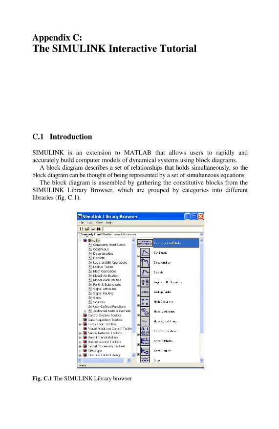
SIMULINK is an extension to MATLAB that allows users to rapidly and accurately build computer models of dynamical systems using block diagrams.
A block diagram describes a set of relationships that holds simultaneously, so the block diagram can be thought of being represented by a set of simultaneous equations.
The block diagram is assembled by gathering the constitutive blocks from the SIMULINK Library Browser, which are grouped by categories into different libraries (fig. C.1).
Fig. C.1 The SIMULINK Library browser

214 Appendix C: The SIMULINK Interactive Tutorial
In order to access SIMULINK we can type in the MATLAB command window >> SIMULINK
or else click on the SIMULINK icon (fig. C.2)
Fig. C.2 The access to SIMULINK from MATLAB
Once we access SIMULINK a new model must be created by dragging blocks from the SIMULINK Library browser to this new model window, by selecting the appropriate library where the searched block is included.
Fig. C.3 The SIMULINK Block Library
For the purpose of modeling, simulation, and control of dynamic systems, a subset of SIMULINK libraries will be used, namely, Continuous, Discontinuities, Lookup

C.2 Creating a Model 215
Tables, Math Operations, Ports and Subsystems, Signal Routing, Sinks, Sources, User-Defined Functions and Additional Linear (included into SIMULINK Extras) (fig. C.3)
C.2 Creating a Model
In order to explain the process followed to create a SIMULINK model, we have selected a simple feedback control system for a ship (fig. C.4).
Fig. C.4 Feedback control system for a ship
In the first place we have to collect all blocks necessary to build the system from the SIMULINK block Library. Afterwards, we will connect the selected blocks to implement the block diagram, also changing the parameters of these blocks if it is necessary. Finally the system is simulated by selecting the appropriate solver options.
Therefore, as first step, we open a new model, dragging the constitutive blocks of the block diagram from each one of the block libraries where they are included (fig. C.5)
Fig. C.5 Building process for the feedback control of a ship (step 1)

216 Appendix C: The SIMULINK Interactive Tutorial
As second step, we connect these blocks following the desired connection pattern as indicated in the feedback control system (fig. C.6). Possibly, it will be necessary to flip or rotate some blocks or to derive some pickoff points.
Fig. C.6 Building process for the feedback control of a ship (step 2)
Fig. C.7 Building process for the feedback control of a ship (step 3)
Afterword, in a third step we have to change the block’s parameters according to the values defined in the original feedback control system if it is necessary, adding optionally labels both to identify the signals transferred between blocks or to name specific blocks (fig. C.7). Block parameters can also be defined from the MATLAB workspace and used in SIMULINK. In this case we have assigned the gains, maxim saturation, and reference step as >> Kd=1.8; >> Kp=1.5;

C.2 Creating a Model 217
>> Lsat=10; >> phir=90;
Before simulation is run, we must select the appropriate simulation time and the numerical method used, including the integration step value in case of fixed-step selection (fig. C.8).
Fig. C.8 Definition of the solver configuration for the feedback control.
Fig. C.9 Step response of the DC motor obtained by using SIMULINK
Finally, the simulation is run by double-clicking on the icon and output responses can be viewed by double-clicking on the Scope block to view its output. Hit the auto-scale button to see the step response of the feedback controller applied to a reference course for a step amplitude of 90 (fig. C.9)

218 Appendix C: The SIMULINK Interactive Tutorial
C.3 SIMULINK Libraries
SIMULINK contains a large number of blocks from which models can be built. These blocks are arranged in Block Libraries which are accessed by the main SIMULINK window.
The set of Block Libraries we are going to describe contains the main blocks used for analysis, modeling and control of dynamic system, nonlinear in general. We will only focus on the blocks which have been used throughout the text, leaving aside other blocks less used in the System Engineering field.
C.3.1 Continuous Library
This section is an introduction to the Continuous Library of SIMULINK. We will describe the function of some blocks included in this library (fig. C.10)
Fig. C.10 The SIMULINK Continuous Library

C.3 SIMULINK Libraries 219
Integrator
The Integrator block integrates its input and is used with continuous−time signals. We can use different numerical integration methods to compute the Integrator block's output.
Transfer Function
The Transfer Fcn block implements a transfer function as a ratio of polynomials.
Zero-Pole
The Zero-Pole block implements a system with the specified zeros, poles, and gain in the s domain.
State-Space
The State-Space block implements a system defined by the state-space equations.
Derivative
The Derivative block approximates the derivative of its input. The initial output for the block is zero. The accuracy of the results depends on the size of the time steps taken in the simulation.
Transport Delay

220 Appendix C: The SIMULINK Interactive Tutorial
The Transport Delay block delays the input by a specified amount of time. It can be used to simulate a time delay.
C.3.2 Source Library
This section is an introduction to the Source Library of SIMULINK. We will describe the function of some blocks included in this library (fig. C.11).
Fig. C.11 The SIMULINK Source Library

C.3 SIMULINK Libraries 221
Constant block
The Constant block is used to define a real or complex constant value. This block accepts scalar, vector, or matrix. Step
The Step block generates a step between two defined levels at some specified time. Ramp
The Ramp block generates a signal that starts at a specified time and value and changes by a specified rate. The characteristics of the generated signal are determined by the specified Slope and Start time. Sine Wave
The Sine Wave block generates a sine wave. To generate a cosine wave, we specify the Phase parameter as .
Pulse Generator
The Pulse Generator block generates square wave pulses at regular intervals. The shape of the generated waveform depends on the parameters, Amplitude, Pulse Width, Period, and Phase Delay as shown in (fig. C.12).

222 Appendix C: The SIMULINK Interactive Tutorial
Fig. C.12 Illustration of the Pulse Generator block parameters
Signal Builder
The Signal Builder block allows the user to create interchangeable groups of piece-wise linear signal sources.
Digital Clock
The Digital Clock block displays the simulation time at a specified sampling interval.
From File
The From File block outputs data read from a MAT file. The name of the file is displayed inside the block.
From Workspace
The From Workspace block reads data from the MATLAB workspace.

C.3 SIMULINK Libraries 223
Signal Generator
The Signal Generator block can produce one of four different waveforms: sine wave, square wave, saw tooth wave, and random wave.
C.3.3 Sinks Library
This section is an introduction to the Sinks Library of SIMULINK. We will describe the function of some blocks included in this library (fig. C.13).
Fig. C.13 The SIMULINK Sinks Library
Scope
The Scope block displays its input with respect to simulation time. The Scope block can have multiple axes (one per port), but all axes have a common time

224 Appendix C: The SIMULINK Interactive Tutorial
range with independent y−axes. We can move and resize the Scope window and we can modify the Scope's parameter values during the simulation.
Display
The Display block shows the value of its input on its icon. The display formats are the same as those of MATLAB.
XY Graph
The XY Graph block displays an X−Y plot of its inputs in a MATLAB figure window. This block plots data in the first input (the x direction) against data in the second input (the y direction).
To File
The To File block writes its input to a matrix in a MAT−file. The block writes one column for each time step: the first row is the simulation time; the remainder of the column is the input data.
To Workspace
The To Workspace block writes its input to the workspace. This block writes its output to an array or structure that has the name specified by the block's Variable name parameter. The Save format parameter determines the output format.
Stop Simulation
The Stop Simulation blocks the simulation when the input signal is “TRUE”.
C.3 SIMULINK Libraries 225
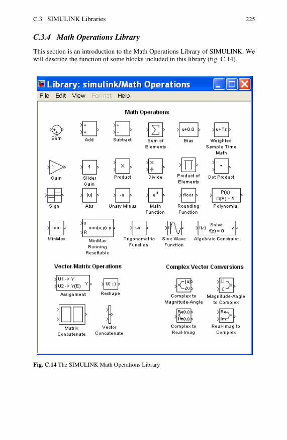
C.3.4 Math Operations Library
This section is an introduction to the Math Operations Library of SIMULINK. We will describe the function of some blocks included in this library (fig. C.14).
Fig. C.14 The SIMULINK Math Operations Library

226 Appendix C: The SIMULINK Interactive Tutorial
Sum
The Sum block is an implementation of the Add block which is described below. We can choose the icon shape (round or rectangular) of the block on the Block Parameters dialog box. Add
The Add block performs addition or subtraction on its inputs. This block can add or subtract scalar, vector, or matrix inputs. We specify the operations of the block with the list of sign parameters, plus (+), minus (-). Gain
The Gain block multiplies the input by a constant value (gain). The input and the gain can each be a scalar, vector, or matrix. Product block
The Product block performs multiplication or division of its inputs. We specify the operations with the number of inputs parameter. Multiply (*) and divide (/) characters indicate the operations to be performed on the inputs. Divide
The Divide block is an implementation of the Product block. It can be used to multiply or divide inputs.
C.3 SIMULINK Libraries 227
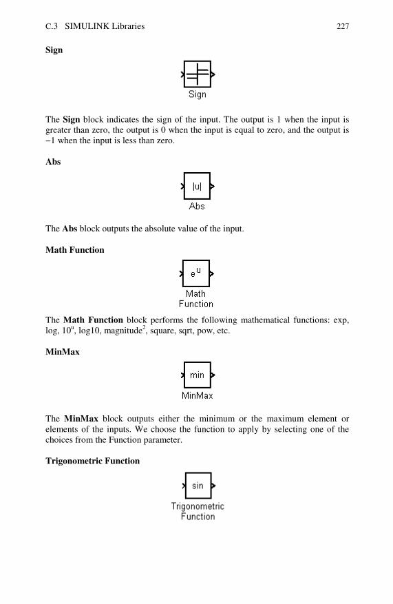
Sign
The Sign block indicates the sign of the input. The output is 1 when the input is greater than zero, the output is 0 when the input is equal to zero, and the output is −1 when the input is less than zero. Abs
The Abs block outputs the absolute value of the input. Math Function
The Math Function block performs the following mathematical functions: exp, log, 10u, log10, magnitude2, square, sqrt, pow, etc. MinMax
The MinMax block outputs either the minimum or the maximum element or elements of the inputs. We choose the function to apply by selecting one of the choices from the Function parameter. Trigonometric Function

228 Appendix C: The SIMULINK Interactive Tutorial
The Trigonometric Function block performs the trigonometric functions sin, cos, tan, asin, acos, atan, and the hyperbolic functions sinh, cosh, tanh, asinh, acosh, and atanh.
C.3.5 Lookup Table Library
This section is an introduction to the Lookup Table Library of SIMULINK. We will describe the function of some blocks included in this library (fig. C.15).
Fig. C.15 The SIMULINK Lookup Tables Library Lookup Table
The Lookup Table block computes an approximation to a function where the data vectors x and y are given, and it is required that the x data vector must be monotonically increasing.
Lookup Table (2−D)

C.3 SIMULINK Libraries 229
The Lookup Table (2−D) block computes an approximation for a function , when the data points x, y, and z are given. Lookup Table (n−D)
The Lookup Table (n−D) block n−dimensional interpolated table lookup including index searches. The table is a sample representation of a function of N variables.
C.3.6 Discontinuities Library
This section is an introduction to the Discontinuities Library of SIMULINK. We will describe the function of some blocks included in this library (fig. C.16).
Fig. C.16 The SIMULINK Discontinuities Library
230 Appendix C: The SIMULINK Interactive Tutorial
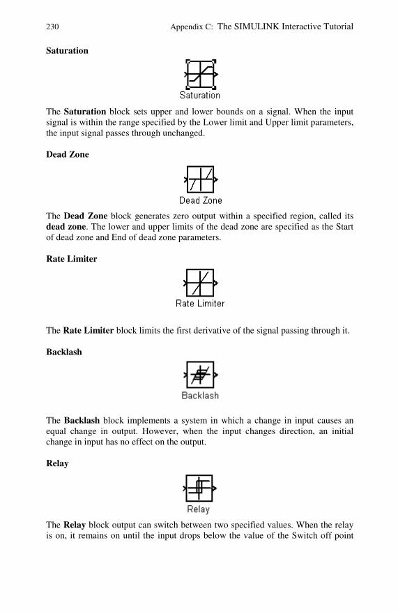
Saturation
The Saturation block sets upper and lower bounds on a signal. When the input signal is within the range specified by the Lower limit and Upper limit parameters, the input signal passes through unchanged. Dead Zone
The Dead Zone block generates zero output within a specified region, called its dead zone. The lower and upper limits of the dead zone are specified as the Start of dead zone and End of dead zone parameters. Rate Limiter
The Rate Limiter block limits the first derivative of the signal passing through it. Backlash
The Backlash block implements a system in which a change in input causes an equal change in output. However, when the input changes direction, an initial change in input has no effect on the output. Relay
The Relay block output can switch between two specified values. When the relay is on, it remains on until the input drops below the value of the Switch off point

C.3 SIMULINK Libraries 231
parameter. When the relay is off, it remains off until the input exceeds the value of the Switch on point parameter.
C.3.7 Signal Routing Library
This section is an introduction to the Signal Routing Library of SIMULINK. We will describe the function of some blocks included in this library (fig. C.17).
Fig. C.17 The SIMULINK Signal Routing Library Mux

232 Appendix C: The SIMULINK Interactive Tutorial
The Mux block combines its inputs into a single output. An input can be a scalar, vector, or matrix signal. Demux
The Demux block extracts the components of an input signal and outputs the components as separate signals. Switch
The Switch block outputs the first (top) input or the third (bottom) input depending on the value of the second (middle) input. The first and third inputs are the data inputs. The second input is the control input. From
The From block accepts a signal from a corresponding Goto block , and passes it as output. Goto
The Goto block passes its input to its corresponding From blocks. From and Goto blocks allow us to pass a signal from one block to another without actually connecting them.
C.3.8 Ports and Subsystems Library
This section is an introduction to the Ports and Subsystems Library of SIMULINK. We will describe the function of some blocks included in this library (fig. C.18).

C.3 SIMULINK Libraries 233
Fig. C.18 The SIMULINK Ports and Subsystems Library

234 Appendix C: The SIMULINK Interactive Tutorial
Inport, Outport, and Subsystem
Inport blocks are ports that serve as links from outside a system into the system. Outport blocks are output ports for a subsystem. A Subsystem block represents a subsystem of the system that contains it. As our model increases in size and complexity, we can simplify it by grouping blocks into subsystems.
C.3.9 User-Defined Functions Library
This section is an introduction to the User-defined Functions Library of SIMULINK. We will describe the function of some blocks included in this library (fig. C.19).
Fig. C.19 The SIMULINK User-defined Functions Library
Fcn
C.3 SIMULINK Libraries 235
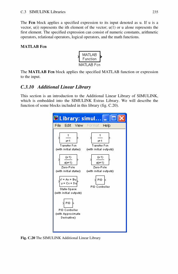
The Fcn block applies a specified expression to its input denoted as u. If u is a vector, u(i) represents the ith element of the vector; u(1) or u alone represents the first element. The specified expression can consist of numeric constants, arithmetic operators, relational operators, logical operators, and the math functions. MATLAB Fcn
The MATLAB Fcn block applies the specified MATLAB function or expression to the input.
C.3.10 Additional Linear Library
This section is an introduction to the Additional Linear Library of SIMULINK, which is embedded into the SIMULINK Extras Library. We will describe the function of some blocks included in this library (fig. C.20).
Fig. C.20 The SIMULINK Additional Linear Library

236 Appendix C: The SIMULINK Interactive Tutorial
Transfer Fcn (with initial states)
Transfer Fcn (with initial output)
Zero-Pole (with initial states)
Specify the initial output for the transfer function as a ratio of polynomials. Zero-Pole (with initial ouput)
Specify the initial output for the transfer function given by zero, pole, and gain format. States-Space (with initial ouput)
Specify the initial output for the system given in state space format.

C.3 SIMULINK Libraries 237
PID Controller
Implements the proportional-integral-derivative action based on the proportional, integral and derivative gains. PID Controller (with Approximate Derivative)
Implements the proportional-integral-derivative action, with derivative term implemented using an s/(s/N +1) transfer function block.

Appendix D: The SIMSCAPE Modeling Environment Tutorial
Appe ndix DThe SIMSCAP E Mo deling Env ironment Tutoria l
Appendix D
D.1 Introduction
SIMSCAPE is a MATLAB-based, object-oriented physical modeling language that enables the user to create models of physical components using an acausal modeling approach.
This language is designed for use in the MATLAB and SIMULINK environments, for it can benefit MATLAB functions and SIMULINK blocks (fig. D.1).
Fig. D.1 The SIMULINK Library browser

240 Appendix D: The SIMSCAPE Modeling Environment Tutorial
The integration of control systems with physical systems covering multiple physical domains such as electrical, mechanical, hydraulic, etc., requires a useful model representation of the physical system. The physical network approach enables the users to create models of physical components that can cover multiple physical domains and can also be reusable.
The SIMSCAPE methodology is based on the connection of physical components, each one with its dynamic equations embedded. The specific connection diagram together with the conservation laws applied, determines the system dynamic equations.
The physical component diagram is assembled by gathering the constitutive components from the Foundation Library of the SIMSCAPE Library Browser, which can be accessed from the SIMULINK Library Browser (fig. D.2). The SIMSCAPE components are grouped by categories into different libraries of components (Electrical, Hydraulic, Mechanical, Physical Signals, Thermal) and Utilities.
Fig. D.2 The SIMSCAPE Library browser
D.2 Creating a Model 241
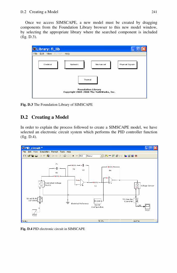
Once we access SIMSCAPE, a new model must be created by dragging components from the Foundation Library browser to this new model window, by selecting the appropriate library where the searched component is included (fig. D.3).
Fig. D.3 The Foundation Library of SIMSCAPE
D.2 Creating a Model
In order to explain the process followed to create a SIMSCAPE model, we have selected an electronic circuit system which performs the PID controller function (fig. D.4).
Fig. D.4 PID electronic circuit in SIMSCAPE

242 Appendix D: The SIMSCAPE Modeling Environment Tutorial
In first place we have to collect all components necessary to build the PID controller from the Foundations Library. Afterwards, we will connect the selected components to implement the physical components diagram, also changing the parameters of these components if it is necessary. Finally the system is simulated by selecting the appropriate solver options.
Therefore, as first step, we open a new component model, dragging the constitutive components of the physical components diagram from each one of the components libraries where they are included (fig. D.5).
As second step, we connect these components following the desired connection pattern as indicated in the PID electronic circuit (fig. D.6). Possibly, it will be necessary to flip or rotate some components or to derive some pickoff points.
Afterward, in a third step we have to change the component’s parameters according to the values defined in the original PID electronic circuit if it is necessary, adding optionally labels both to identify the signals transferred between components or to name specific components (fig. D.7). Component parameters can also be defined from the MATLAB workspace and used in SIMSCAPE. In this case we have assigned the resistors, capacitors, gains, and ramp slope values as >> R1=153.85*10^3; >> R2=153.85*10^3; >> R3=10*10^3; >> R4=197.1*10^3; >> C1=10*10^-6; >> C2=10*10^-6; >> ramp_slope=0.1;
Fig. D.5 Building process for the PID circuit (step 1)
D.2 Creating a Model 243
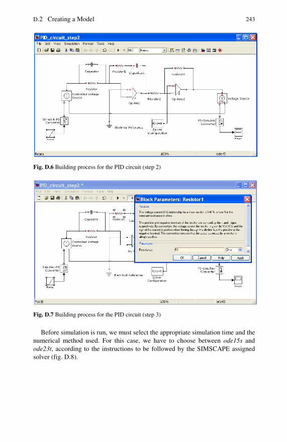
Fig. D.6 Building process for the PID circuit (step 2)
Fig. D.7 Building process for the PID circuit (step 3)
Before simulation is run, we must select the appropriate simulation time and the numerical method used. For this case, we have to choose between ode15s and ode23t, according to the instructions to be followed by the SIMSCAPE assigned solver (fig. D.8).

244 Appendix D: The SIMSCAPE Modeling Environment Tutorial
Fig. D.8 Definition of the solver configuration for the PID circuit.
Finally, the simulation is run by double-clicking on the icon and output responses can be viewed by double-clicking on the Scope block to view its output. Hit the auto-scale button to see the ramp response of the PID circuit controller for a ramp slope of 0.1 (fig. D.9).
Fig. D.9 Ramp response of the PID using SIMSCAPE
D.3 SIMSCAPE Libraries
SIMSCAPE contains a large number of components from which physical models can be built. These components are arranged in Components Libraries which are accessed by the main SIMULINK window.

D.3 SIMSCAPE Libraries 245
The set of Component Libraries we are going to describe contains the main blocks used for analysis, modeling and control of dynamic systems, mainly composed of electrical, hydraulic, mechanical, and thermal components, together with physical signal blocks utilized to define components with more complicated physical relations.
D.3.1 Electrical Library
This section is an introduction to the Electrical Library of SIMSCAPE. We will illustrate the components included in this library (fig. D.10).
Fig. D.10 The SIMSCAPE Electrical Library
The Electrical Library is composed of three sub-libraries, termed the Electrical Elements, Electrical Sensors, and Electrical Sources libraries.
Fig. D.11 The SIMSCAPE Electrical Elements sub-library
The Electrical Elements library contains some of the common elements which constitute the electric and electronic networks, both linear (capacitor, inductance, resistance, etc.) and nonlinear (diode, switch, etc.) together with the electromechanical converters (fig. D.11).
The Electrical Sensors library contains both a voltage and a current sensor to be placed in parallel or series with the element whose magnitude is being measured (fig. D.12).

246 Appendix D: The SIMSCAPE Modeling Environment Tutorial
Fig. D.12 The SIMSCAPE Electrical Sensors sub-library
The Electrical Source library contains both voltage and current (AC and DC) sources, either fixed or voltage/current controlled to be used as electric sources for the model (fig. D.13).
Fig. D.13 The SIMSCAPE Electrical Sources sub-library
D.3.2 Hydraulic Library
This section is an introduction to the Hydraulic Library of SIMSCAPE. We will illustrate the components included in this library (fig. D.14).
Fig. D.14 The SIMSCAPE Hydraulic Library
The Hydraulic Library is composed by three sub-libraries, termed the Hydraulic Elements, Hydraulic Sensors and Actuators, and Hydraulic Utilities libraries.

D.3 SIMSCAPE Libraries 247
The Hydraulic Elements library contains some of the common elements which constitute the hydraulic circuits (resistance, inertance, capacitance,..) together with the hydromechanical converters (pump and piston) (fig. D.15).
Fig. D.15 The SIMSCAPE Hydraulic Elements sub-library
The Hydraulic Sensors and Actuators library contains both pressure and flow sensors and sources in order to measure or actuate over the hydraulic circuit elements (fig. D.16).
Fig. D.16 The SIMSCAPE Hydraulic Sensors and Actuators sub-library
Finally, a element to define the characteristics of fluid used by the hydraulic circuit is also included, into the Hydraulic Uilities library (fig. D.17)
Fig. D.17 The SIMSCAPE Hydraulic Utilities sub-library
248 Appendix D: The SIMSCAPE Modeling Environment Tutorial
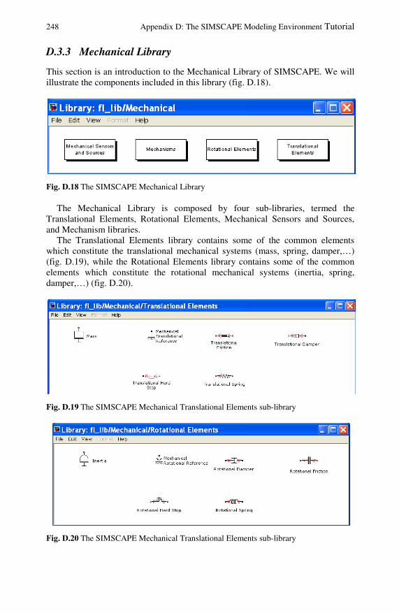
D.3.3 Mechanical Library
This section is an introduction to the Mechanical Library of SIMSCAPE. We will illustrate the components included in this library (fig. D.18).
Fig. D.18 The SIMSCAPE Mechanical Library
The Mechanical Library is composed by four sub-libraries, termed the Translational Elements, Rotational Elements, Mechanical Sensors and Sources, and Mechanism libraries.
The Translational Elements library contains some of the common elements which constitute the translational mechanical systems (mass, spring, damper,…) (fig. D.19), while the Rotational Elements library contains some of the common elements which constitute the rotational mechanical systems (inertia, spring, damper,…) (fig. D.20).
Fig. D.19 The SIMSCAPE Mechanical Translational Elements sub-library
Fig. D.20 The SIMSCAPE Mechanical Translational Elements sub-library

D.3 SIMSCAPE Libraries 249
The Mechanical Sensors and Sources library contains both translational and rotational position/velocity sensors as well as force/torque sensors. Besides, contains force/torque sources in order to actuate over the mechanical circuit elements, as well as velocity sources (fig. D.21).
Fig. D.21 The SIMSCAPE Mechanical Sensors and Sources sub-library
Additionally, a Mechanism library where mechanical transformers (gear and lever) and ideal pulleys can be found, is included (fig. D.22).
Fig. D.22 The SIMSCAPE Mechanisms sub-library
D.3.4 Thermal Library
This section is an introduction to the Thermal Library of SIMSCAPE. We will illustrate the components included in this library (fig. D.23).
Fig. D.23 The SIMSCAPE Thermal Library

250 Appendix D: The SIMSCAPE Modeling Environment Tutorial
The Thermal Library is composed of two sub-libraries, termed the Thermal Elements, and Thermal Sensors and Sources libraries.
The Thermal Elements library contains some of the common elements which constitute the thermal systems (mass and heat trasnfer mechanism) (fig. D.24).
Fig. D.24 The SIMSCAPE Thermal Elements sub-library
The Thermal Sensors and Sources library contains both tempearture and heat flow sensors and sources in order to measure or actuate over the thermal circuit elements (fig. D.25).
Fig. D.25 The SIMSCAPE Thermal Sensors and Sources sub-library
D.3.5 Physical Signal Library
This section is an introduction to the Physical Signal Library of SIMSCAPE, which is utilized to create equations, by using linear and nonlinear operators, functions, lookup tables, etc. These equations are solved simultaneously with physical system, and unit conversions are handled automatically.
We will illustrate the blocks included in this library and its function (fig. D.26). These blocks are similar to those described in the SIMULINK Libraries, and perform the same function, by using physical signal instead of dimensionless variables as SIMULINK. In this way, it includes linear blocks (adder, gain, integrator,…) and nonlinear also (divider, math function, table lookup, saturation,…) as it is shown in fig. D.27.

D.3 SIMSCAPE Libraries 251
Fig. D.26 The SIMSCAPE Physical Signals Library
Fig. D.27 Blocks included into the SIMSCAPE Physical Signals Library
D.3.6 Utilities Library
This section is an introduction to the Utilities Library of SIMSCAPE, which contains general purpose blocks as the PSS and SPS converters from SIMSCAPE to SIMULINK or vice versa respectively, together with the input/output ports to define subsystems in SIMSCAPE. Additionally, the solver block, which is necessary to be attached to the physical components diagram is included, thus the solver can be applied with the numerical methods to integrate the dynamic system equations (fig. D.28).
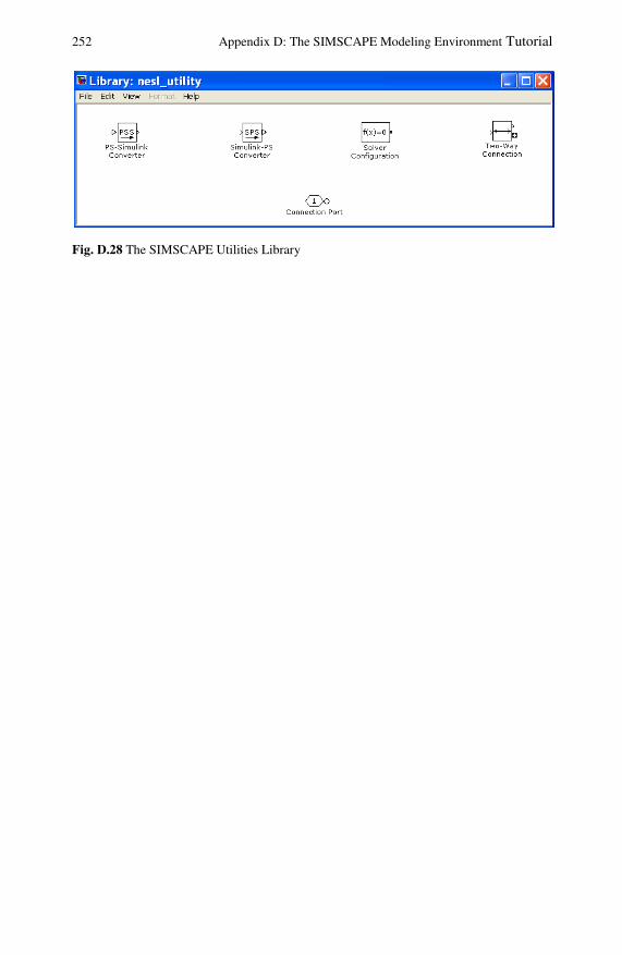
252 Appendix D: The SIMSCAPE Modeling Environment Tutorial
Fig. D.28 The SIMSCAPE Utilities Library

Index
A actuators, 137 B block diagrams, 76
reduction rules, 79
C
compensator. See gain control systems
proportional control, 108 Control systems, 137
bang-bang control, 140 closed loop systems, 138 controller, 138 integral control, 146 open loop systems, 139 PID Control, 142 Proportional control, 144
Control Systems Derivative control, 148
D
damping ratio, 100 E Electrical Systems, 19 error, 5, 107
position constant, 133 steady-state error, 131 velocity constant, 134
G
gain, 89, 158
H
Hydraulic Systems, 30
I initial conditions, 62
L
Laplace transform, 51
Final value theorem, 54 inverse transform, 55 properties, 52
M
Matlab commands
ginput, 155 initial, 88 lsim, 88 residue, 94 rlocus, 117 rltool, 158 roots, 127 step, 88
Mechanical Systems, 24
N
natural frequency, 100
P
Perturbations, 138 poles, 63, 93
dominance of, 106

254 Index
R
Response, 85 forced response, 86 natural response, 86 steady-state response, 85 transient response, 85
root locus technique, 107 angle condition, 110 asymptotes, 113 magnitude condition, 110 rupture points, 114
S
sensors, 137 Simulink Blocks
Abs, 227 Add, 226 Backlash, 230 Constant source, 221 Dead Zone, 230 Demux, 232 Derivative, 219 Digital clock, 222 Dispaly, 224 Divide, 226 Fcn, 234 From, 232 From file block source, 222 From workspace block source, 222 Gain, 226 Goto, 232 Inport, Outport, Subsystem, 234 Integrator, 219 Look table nD, 229 Lookup table, 228 Lookup table 2D, 228 Math function, 227 Matlab Fcn, 235 MinMax, 227 Mux, 231 PID controller, 237 PID controller (approximate
derivative), 237 Product, 226 Pulse Generator, 221 Ramp, 221 Rate Limiter, 230 Relay, 230 Saturation, 230 Scope, 223
Sign, 227 Signal builder, 222 Signal Generator, 223 Sine wave source, 221 State-Sapce (initial outputs), 236 State-Space, 219 Step, 221 Stop simulation, 224 Sum, 226 Switch, 232 To file block sink, 224 To workspace block sink, 224 Transfer Fcn (initial outputs), 236 Transfer Fcn (initial states), 236 Transfer function, 219 Transport Delay, 219 Trigonometric function, 227 XY Graph, 224 Zero-Pole, 219 Zero-Pole (initial outputs), 236 Zero-Pole (initial states), 236
stability, 126 Routh-Hürwitz theorem, 128
State Space, 67 state, 67 state equations, 69
system, 1 closed loop systems, 4, 138 continuous systems, 3 control systems, 5 critically damped systems, 101 deterministic system, 3 discrete systems, 3 dynamic systems, 3 event discrete systems, 4 First-order systems, 87 High-order systems, 105 Linear and Invariant Time systems,
45 linear and time invariant (LTI), 43 modeling, 13 multi-input multi-output systems, 67 multi-input, multi-output systems, 44 open loop systems, 4, 139 overdamped systems, 101 Second-order systems, 92 static systems, 2 stochastic systems, 3 type of a, 132
System identification, 121 First-order system identification, 121 Overshoot, 123

Index 255 Peak time, 123 Rise time, 123 Second-order system identification,
122 Settling time, 123 Steady state value, 124
System Simulation, 167 SIMSCAPE, 167 SIMULINK, 167
Systems description, 5 external description, 6 internal description, 8
Systems linearization, 46
T Thermal Systems, 33 time constant, 90 transfer function, 62
Z zeros, 63 Ziegler-Nichols techniques, 150
closed loop, 153 open loop, 151

![Washington, D.C. 20230 q]fffp](https://img.pdfslide.us/doc/110x75/6257bfc49a43555608096d0b/washington-dc-20230-qfffp.jpg)