APPENDIX A SAMPLING AND INSTRUMENTATION EQUIPMENT … · SAMPLING AND INSTRUMENTATION EQUIPMENT 1. ... 4. 36 x 28 x 1 in. ... to log-Tchebycheff rule TABLE B-1

A-1

APPENDIX A

SAMPLING AND INSTRUMENTATION EQUIPMENT

A-2

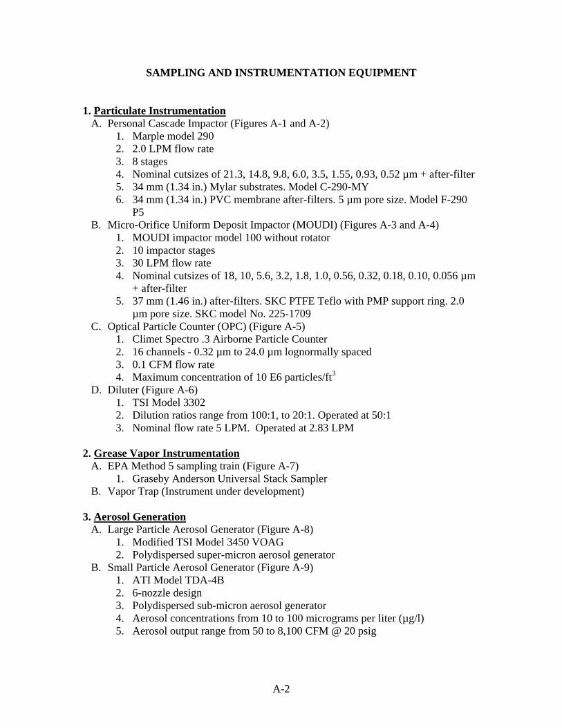
SAMPLING AND INSTRUMENTATION EQUIPMENT 1. Particulate Instrumentation

A. Personal Cascade Impactor (Figures A-1 and A-2) 1. Marple model 290 2. 2.0 LPM flow rate 3. 8 stages 4. Nominal cutsizes of 21.3, 14.8, 9.8, 6.0, 3.5, 1.55, 0.93, 0.52 µm + after-filter 5. 34 mm (1.34 in.) Mylar substrates. Model C-290-MY 6. 34 mm (1.34 in.) PVC membrane after-filters. 5 µm pore size. Model F-290

P5 B. Micro-Orifice Uniform Deposit Impactor (MOUDI) (Figures A-3 and A-4)

1. MOUDI impactor model 100 without rotator 2. 10 impactor stages 3. 30 LPM flow rate 4. Nominal cutsizes of 18, 10, 5.6, 3.2, 1.8, 1.0, 0.56, 0.32, 0.18, 0.10, 0.056 µm

+ after-filter 5. 37 mm (1.46 in.) after-filters. SKC PTFE Teflo with PMP support ring. 2.0

µm pore size. SKC model No. 225-1709 C. Optical Particle Counter (OPC) (Figure A-5)

1. Climet Spectro .3 Airborne Particle Counter 2. 16 channels - 0.32 µm to 24.0 µm lognormally spaced 3. 0.1 CFM flow rate 4. Maximum concentration of 10 E6 particles/ft3

D. Diluter (Figure A-6) 1. TSI Model 3302 2. Dilution ratios range from 100:1, to 20:1. Operated at 50:1 3. Nominal flow rate 5 LPM. Operated at 2.83 LPM

2. Grease Vapor Instrumentation

A. EPA Method 5 sampling train (Figure A-7) 1. Graseby Anderson Universal Stack Sampler

B. Vapor Trap (Instrument under development) 3. Aerosol Generation

A. Large Particle Aerosol Generator (Figure A-8) 1. Modified TSI Model 3450 VOAG 2. Polydispersed super-micron aerosol generator

B. Small Particle Aerosol Generator (Figure A-9) 1. ATI Model TDA-4B 2. 6-nozzle design 3. Polydispersed sub-micron aerosol generator 4. Aerosol concentrations from 10 to 100 micrograms per liter (µg/l) 5. Aerosol output range from 50 to 8,100 CFM @ 20 psig

A-3

4. Sampling Probes A. 2-stage isokinetic sampling probe, brass tapered inlet nozzle, 4.00 in. (101.6 mm)

bend radius. Probe for OPC, PCI, and MOUDI sampling. (Figures A-10 to A-15) B. In-duct isokinetic sampling probe (Figures A-16 and A-17)

1. Used in spatial uniformity tests 2. 13 markings along shaft at specific points for measuring probe in-duct

location C. Small sampling probe. Probe for EPA Method 5 sampling. (Figure A-18)

5. Griddle

A. Electric Griddle 1. Wolf Range Co. Model TME-36A 2. 47.5 amperes @ 208 V 3. 3 phase service 4. 36 x 28 x 1 in. (91.44 x 71.12 x 2.54 cm) cooking surface 5. 6 electric heater elements

6. Neutralization

A. Neutralization Assembly 1. Staticmaster (Figures A-19 and A-20)

a. 6- Model 2U500 b. Po210 ionizing unit c. Designed to bring aerosol charge to Boltzmann equilibrium

2. PVC Housing (Figure A-21) 7. Temperature

A. Type K thermocouple array. 20 gauge wire, glass braid insulation (900 °F, 482 °C) B. Digital multimeter with Type K thermocouple capability

1. Keithley Model 2700 Multimeter/Data Acquisition System 8. Duct Velocity Measurements

A. Portable hot-wire anemometer. (Figure A-22) 1. TSI model 8330 VelociCheck

B. Aerosol Sampling Probe with holder (Figure A-23) 9. Barometric Pressure

A. Manometer. Curtin Matheson Scientific Nova 10. Flow Measurements

A. Digital bubble flow meter (for calibrating EPA Method 5 and diluter flow rates) (Figure A-24)

1. Gilian Gilibrator 2 Control Base PN: 850190 2. Gilian Bubble Generator, range: 0-6000 cc/min PN: D800286 3. Gilian Bubble Generator, range: 0-250 cc/min PN: D800287

B. Dry Gas Meter (for calibrating MOUDI flow rate)

A-4

11. Relative Humidity

A. Portable humidity/temperature sensor. Vaisala model HMI 31 indicator unit, HMP-35 probe

12. Analytic

A. Analytic micro-balance. Cahn C-31, 0 – 250 mg, 0.1 µg resolution B. Fine analytic balance. Sartorius B-120 S, 0 – 110 g, 0.1 mg resolution C. Coarse analytic balance. Sartorius L-610, 0 – 610 g, 0.01 g resolution D. Gateway computer with serial port connection

13. Pictures and Schematic Drawings

Figure A-1. Components of the Model 290 Marple impactor

Note: The collection substrates and after-filter are not pictured. Mylar substrates were used, and the after-filter was a PVC membrane.

A-5

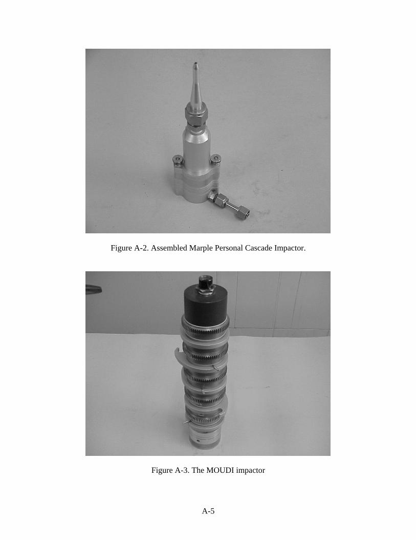
Figure A-2. Assembled Marple Personal Cascade Impactor.

Figure A-3. The MOUDI impactor

A-6

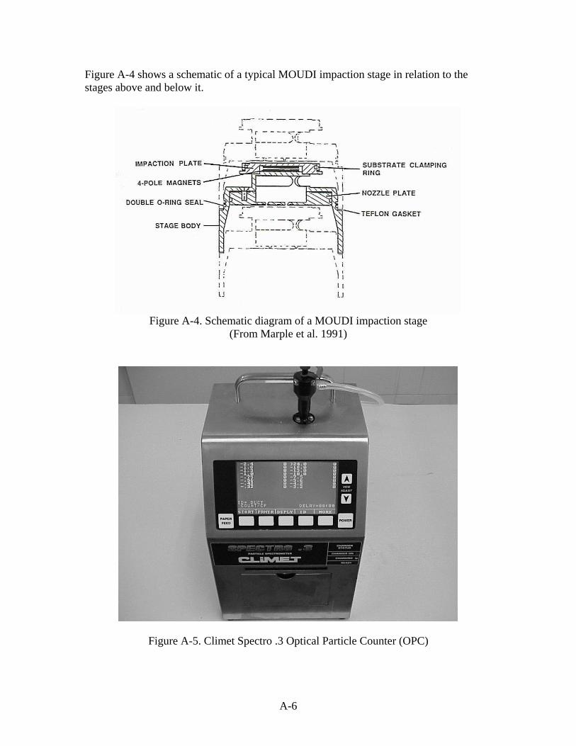
Figure A-4 shows a schematic of a typical MOUDI impaction stage in relation to the stages above and below it.

Figure A-4. Schematic diagram of a MOUDI impaction stage

(From Marple et al. 1991)

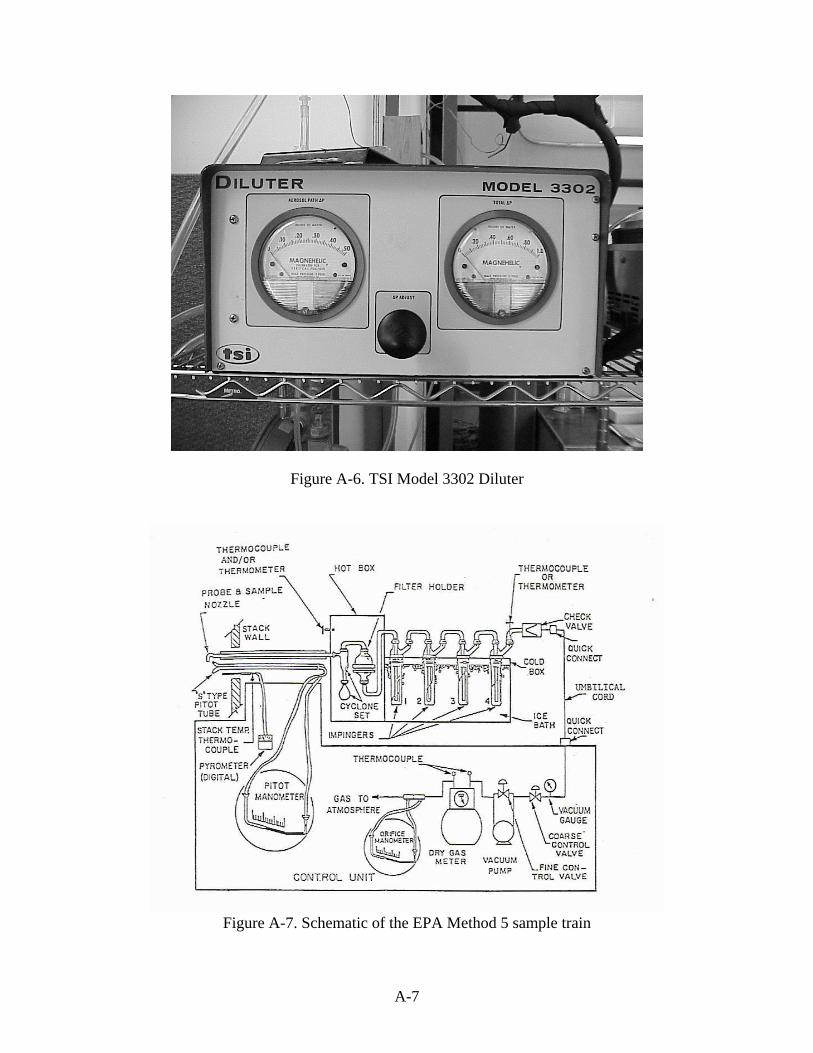
Figure A-5. Climet Spectro .3 Optical Particle Counter (OPC)

A-7

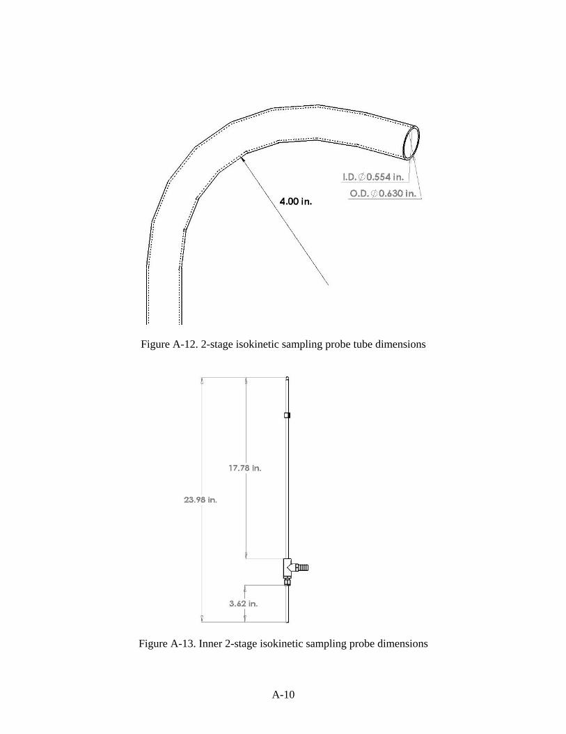
Figure A-6. TSI Model 3302 Diluter

Figure A-7. Schematic of the EPA Method 5 sample train

A-8

Figure A-8. Modified TSI Large Particle Aerosol Generator

Figure A-9. ATI Small Particle Aerosol Generator

A-9

Figure A-10. 2-stage isokinetic sampling probe assembly

Figure A-11. 2-stage isokinetic sampling probe nozzle

A-10

Figure A-12. 2-stage isokinetic sampling probe tube dimensions

Figure A-13. Inner 2-stage isokinetic sampling probe dimensions

A-11

Figure A-14. Inner 2-stage isokinetic sampling probe upper detail

Figure A-15. Inner 2-stage isokinetic sampling probe lower detail

A-12

Figure A-16. Isokinetic probe for aerosol spatial uniformity tests

Figure A-17. Isokinetic probe detail

A-13

Figure A-18. Small sampling probe for EPA Method 5 sampling

Figure A-19. Staticmaster Model 2U500 Ionizing Unit

A-14

Figure A-20. Charge neutralizer data [2]

Figure A-21. Schematic diagram of the spray jet atomizer charge neutralizer

A-15

Figure A-22. TSI VelociCheck portable hot-wire anemometer

Figure A-23. Aerosol sampling probe with holder

A-16

Figure A-24. Gilian digital bubble flow meter assembly

B-1

APPENDIX B

EXHAUST HOOD AND MAKEUP AIR FLOW RATE CALIBRATIONS

B-2

EXHAUST HOOD AND MAKEUP AIR FLOW RATE CALIBRATIONS

1. Exhaust Hood Air Flow Rate Calibration The exhaust hood ventilation system is shown in Figure B-1 and Figure B-2. The fan rotation speed is controlled by a variable frequency AC motor controller which is capable of adjusting the frequency from 0 to 60 Hz. in 0.1 Hz. increments. Ventilation airflow rate calibration consists of measuring the average exhaust velocity in the 12 in. diameter duct at a point 7 duct diameters downstream from the 90° elbow and 2 duct diameters upstream of the expansion section. The average exhaust velocity is used to determine the volumetric airflow rate, which is correlated to the controller frequency as well as the centerline velocity.

Figure B-1. Metal-Fab G Series exhaust duct schematic with part numbers

B-3

B-4

To determine the in-duct measurement positions, the log-Tchebycheff Rule was used. First, three holes were drilled into the duct; one along the vertical axis and two at 60° angles to the vertical, clockwise and counterclockwise, respectively. The hot-wire anemometer probe holder was attached to the duct at each hole location and the anemometer was inserted into the end. As shown in Figure B-3, the tube was divided into 3 equal area concentric circles, and velocity measurements were taken at 6 points across the duct traverse where the probe intersected the concentric circles. Velocity measurements were also taken at the centerline of the duct, 6 in. (15.24 cm) from each side wall. Table B-1 shows the position from the side wall inlet opening of each measuring point.

Figure B-3. Measurement locations in exhaust duct according

to log-Tchebycheff rule

TABLE B-1. POSITION OF MEASUREMENTS ACCORDING TO LOG-TCHEBYCHEFF RULE

1 0.384 (0.98)2 1.620 (4.11)3 3.852 (9.78)4 6.000 (15.24)5 8.148 (20.70)6 10.380 (26.37)7 11.616 (29.50)

Distance from side wall inlet opening, in. (cm)Measuring Point

The test protocol was as follows:

1) Turn on griddle and adjust thermostat settings to achieve an average surface temperature of 375 °F. Allow 1 hour to stabilize.

2) Adjust fan frequency to desired setting. Ensure that there are no filters in the

hood.

B-5

3) Close all doors and windows in the lab and set makeup airflow to approximately that required by kitchen ventilation system.

4) Use log-Tchebycheff Rule for velocity in-duct positions. 5) Perform measurements in triplicate. 6) Repeat steps 2-4 for other fan frequencies.

The measurements were made using a hot-wire anemometer. The average velocity is found by arithmetically averaging the velocities. The average airflow rate is determined by multiplying the average velocity by the duct cross-sectional area. During 4 separate tests, measurements were taken as the fan power frequency was varied from 19 to 45 Hz. Then the average airflow rate was determined. Figure B-4 shows the flow rate vs. the fan frequency.

Flow Rate vs Fan Power Frequency

Q duct = 40.889vR2 = 0.9969

0

200

400

600

800

1000

1200

1400

1600

1800

2000

0 5 10 15 20 25 30 35 40 45 50

Fan Power Frequency (Hz)

Flow

Rat

e (C

FM)

No Filters

1000 CFM

24.5

Hz

Figure B-4. Flow Rate vs. Fan Power Frequency using hot-wire anemometer Equation B-1 is the linear fit equation of the flow rate vs. fan frequency from Figure B-4. Qduct = 40.889v (B-1) where Qduct is the average volumetric flow rate in CFM, and v is the fan power frequency in Hz.

B-6

For the requisite 1000 CFM exhaust velocity, the corresponding fan power frequency is 24.5 Hz. This is simply found by dividing 40.889 by Qduct which is 1000 CFM in this case. The centerline velocity is measured at the center of the duct, 6 in. (15.24 cm) from the wall. Test conditions were the same, and the same four fan power frequencies were used. The exhaust flow rate can be set by adjusting the fan power frequency to the desired level determined by Equation B-1 while there are no filters in the hood. However, when filters are installed in the hood Figure B-4 is not longer valid. The pressure drop across the filters reduces the exhaust flow rate. Therefore, when filters are installed in the hood, the duct centerline velocity is measured and increased or decreased to 1381 ft/min by adjusting the fan power frequency. This centerline velocity corresponds to a total duct flow rate of 1000 CFM. A graph showing centerline velocity vs. flow rate is shown in Figure B-5.

Centerline Velocity vs Flow Rate

Q duct = 0.7239V cl

R2 = 0.999

0

200

400

600

800

1000

1200

1400

1600

1800

2000

0 500 1000 1500 2000 2500 3000

Centerline Velocity (ft/min)

Flow

Rat

e (C

FM)

1000 CFM

1381

ft/m

in

Figure B-5. Flow Rate vs. Centerline Velocity using hot-wire anemometer Equation B-2 is a linear fit equation of Figure B-5. Qduct = 0.7239Vcl (B-2) where Qduct is the average volumetric flow rate in CFM, and Vcl is the centerline velocity, as determined by the anemometer, in ft/min.

B-7

Figure B-6 shows typical measured velocities in the duct across the vertical diameter. These data were used to see if the velocities were symmetric about the centerline. The figure also shows the data points in relation to theory.

0 0.1 0.2 0.3 0.4 0.5 0.6 0.7 0.8 0.9 1 1.1-1

-0.5

0

0.5

1

Velocity Profile in Duct

Re = 1.1 x 105 (smooth duct; Schlichting, 1968)Re = 1.37 x 105 data

u/U

r/R Average Velocity = 1325 ft/min fan frequency = 26 HzFlow rate = 1040 CFM

Figure B-6. Velocity profile in duct across vertical diameter

Figure B-7 shows the average velocity profile and data for the vertical, 60º clockwise, and 60º counter-clockwise measurements according to the log-Tchebycheff Rule. These points were taken at a fan power of 19 Hz which corresponds to a flow rate of 750 CFM.

0 0.2 0.4 0.6 0.8 1-1

-0.5

0

0.5

1


overall average60 deg. ClockwiseVertical60 deg. Counter Clockwise

u/U

r/R

Average Velocity = 955 ft/min fan frequency = 19 HzFlow rate = 750 CFM

Figure B-7. Velocity profile in duct with a fan power frequency of 19 Hz.

B-8

Figure B-8 shows the average velocity profile and data for the vertical, 60º clockwise, and 60º counter-clockwise measurements. These points were taken at a fan speed of 26 Hz. This resulted in an average velocity of 1325 ft/min which, when taken times the cross-sectional area, corresponds to a flow rate of 1040 CFM.

0 0.2 0.4 0.6 0.8 1-1

-0.5

0

0.5

1


overall average60 deg ClockwiseVertical60 deg Counter Clockwise

u/U

r/R

Average Velocity = 1325 ft/min fan frequency = 26 HzFlow rate = 1040



0 0.2 0.4 0.6 0.8 1-1

-0.5

0

0.5

1


60 deg. ClockwiseVertical 60 deg. counter clockwise

overall average

u/U

r/R

Average Velocity =1640 ft/min fan frequency = 30 HzFlow rate = 1290 CFM


B-9


0 0.2 0.4 0.6 0.8 1-1

-0.5

0

0.5

1


overall average60 deg ClockwiseVertical60 deg Counter Clockwise

u/U

r/R

Average Velocity = 2320 ft/min fan frequency = 45 HzFlow rate = 1820 CFM


2. Makeup Air Flow Rate Calibration The average velocity in the makeup air duct was determined by measuring the velocity in the duct at 24 points spaced equally across a cross-section of the duct at several different fan power frequencies with the hot-wire anemometer. The measurement locations are shown in Figure B-11.

1 5 9 13 17 21

2 6 10 14 18 22

3 7 11 15 19 23

4 8 12 16 20 24

Figure B-11. Measurement locations in makeup air duct

B-10

These points were arithmetically averaged to find the average velocity. The volumetric flow rate of the makeup air was then determined by taking the average velocity times the cross-sectional area of the duct. If the flow rate was below or above 1000 CFM then the fan power frequency was raised or lowered and the procedure was repeated until the flow rate was approximately 1000 CFM. The calculated flow rate at a fan power frequency of 26 Hz. is shown below.

( )( )( )minft 1002

in. 12ft 1in. 20in. 12ft/min 601rate flow

32

=⎟⎠⎞

⎜⎝⎛=

C-1

APPENDIX C

AEROSOL SPATIAL UNIFORMITY

C-2

AEROSOL SPATIAL UNIFORMITY In order to accurately determine filter collection efficiency with a single point sample, the aerosol particles need to be well mixed and uniformly distributed throughout the duct cross-section at the sample location. To determine the uniformity of the aerosol distribution in the exhaust duct, two series of measurements were made. One set used aerosol with a mass mean diameter near 0.3 microns (small particles) produced by the ATI aerosol generator using 100% oleic acid. The second set used aerosol particles near 5 microns in diameter produced by the Alltech atomizer using a 2:1 mixture of oleic acid and isopropyl alcohol. In each set of tests, data were obtained with and without a set of baffle filters installed in the hood. The aerosol was injected on top of the heated griddle to simulate cooking aerosol. Figure C-1 shows the setup used for the aerosol sampling.

Figure C-1. Schematic of aerosol sampling system The probe inlet was positioned at the centerline of the 12” duct. The probe transported the aerosol sample to the diluter operating at a 50:1 dilution ratio. The output of the diluter was then sent to the optical particle counter. In the exhaust duct, samples were taken 7 duct diameters (7 ft.) downstream of the 90° elbow and 2 duct diameters (2 ft.) upstream of the 12” to 16” expansion section. Twelve measurement points were required in the horizontal and vertical directions according to EPA requirements, as shown in Figure C-2.

C-3

Figure C-2. EPA: Standards of Performance for New Stationary Sources, pp. 210-862. 40 CFR 60 (Rev. July 1, 1987)

The sample points were located at specific distances across each traverse, and velocity measurements were also taken at each location. The distances are shown in Figure C-3.

C-4

Figure C-3. EPA: Standards of Performance for New Stationary Sources, pp. 210-862. 40 CFR 60 (Rev. July 1, 1987)

Table C-1 shows the actual distances measured for a 12 in. (30.48 cm) round duct.

C-5

TABLE C-1. SAMPLE POINT LOCATIONS FOR DUCT AEROSOL SPATIAL UNIFORMITY TESTS

Measuring Point

(Vertical) Measuring Point

(Horizontal) Distance from side wall inlet opening, in. (cm)

1 13 0.252 (0.64 cm) 2 14 0.804 (2.04 cm) 3 15 1.416 (3.60 cm) 4 16 2.124 (5.39 cm) 5 17 3.000 (7.62 cm) 6 18 4.272 (10.85 cm) 7 19 7.728 (19.63 cm) 8 20 9.000 (22.86 cm) 9 21 9.876 (25.09 cm) 10 22 10.584 (26.88 cm) 11 23 11.196 (28.44 cm) 12 24 11.748 (29.84 cm)

Before any spatial uniformity measurements were taken, the aerosol concentration was measured at the centerline of the duct with the aerosol generator located in the center of the griddle for at least 30 minutes to check the stability of the aerosol generators. Figure C-4 shows the small particle aerosol generator time stability without baffles.

Small ParticlesAerosol Source at Center of Griddle

Probe at Centerline

0

20000

40000

60000

80000

100000

120000

0 5 10 15 20 25 30 35

Time, minutes

Part

icle

Cou

nt

.32-.42

.42-.56

.56-.750.75-1.01.0-1.31.3-1.81.8-2.42.4-3.23.2-4.24.2-5.65.6-7.57.5-10.010.0-13.013.0-18.018.0-24.0>24.0

Figure C-4. ATI small particle aerosol generator time stability without baffles

C-6

Figure C-5 shows the modified TSI large particle aerosol generator time stability with baffles.

Large Particle Uniformity Study-Aerosol Source at Center of Griddle, Probe at Centerline

0

100

200

300

400

500

600

700

800

900

1000

1 2 3 4 5 6 7 8 9 10 11 12 13 14 15 16 17 18 19 20 21 22 23 24 25 26 27 28 29 30

Time, minutes

PAR

TIC

LE C

OU

NT

.32-.42

.42-.56

.56-.750.75-1.01.0-1.31.3-1.81.8-2.42.4-3.23.2-4.24.2-5.65.6-7.57.5-10.010.0-13.013.0-18.018.0-24.0>24.0

4.2-5.6 µm Particles

5.6-7.5 µm Particles

Figure C-5. Modified TSI aerosol generator time stability for large particles with baffles

Following procedures outlined in ASHRAE standard 52.2, several aerosol source locations were tested for the spatial uniformity tests. Figure C-6 shows the source locations outlined in 52.2, and Figure C-7 shows the locations that were tested.

Figure C-6. Griddle surface aerosol source locations from ASHRAE 52.2

C-7

Figure C-7. Griddle surface aerosol source locations tested The following test protocol was used for the testing of aerosol spatial uniformity.

1) Set fan power frequency to 24.5 Hz. (without baffles) or 28 Hz. (with baffles) for exhaust duct flow rate of 1000 CFM.

2) Set air handler fan power frequency to 26 Hz. for 1000 CFM makeup air, turn on

filtration system, adjust RH and water heater to heat makeup air. 3) Turn on griddle to stabilize for one hour after cycling commences. 4) Sample background aerosol for 1 minute. 5) Use 100% oleic acid for ATI aerosol generator and 2:1 mixture of oleic acid and

isopropyl alcohol for TSI aerosol generator. 6) Place aerosol generator discharge at specified position on griddle, turn on and run

for 5 minutes prior to sampling in duct. 7) Sample aerosol in duct at centerline for 1 minute. 8) Move probe to top of duct for vertical traverse or far side of duct for horizontal

traverse. 9) Sample for 1 minute. 10) Move probe to next sample location. 11) Repeat steps 9 and 10 for each location.

C-8

12) Move probe back to centerline and take a final 1 minute sample. 13) Turn off atomizer and allow duct to purge for 5 minutes. 14) Sample background at centerline of duct. 15) Move aerosol source to next griddle position and repeat procedures 6 to 14 above.

A. Small Particle Aerosol Spatial Uniformity Figure C-8 shows the standard operating procedure check-sheet for small particle aerosol spatial uniformity tests.

Figure C-8. Standard operating procedure check-sheet for small particles

C-9

Figure C-9 shows the 25 points that were used for the spatial uniformity tests. These points are identical to the points used for the kitchen hood ventilation rate calibration outlined in appendix B.

Figure C-9. Sampling locations in exhaust duct for small particles without baffles

1. Small Particles - Without Baffles

Figures C-10 and C-11 show the aerosol spatial uniformity of small particles without baffles with the aerosol source at the center of the griddle along the vertical and horizontal traverses, following the test protocol outlined above.

C-10

AEROSOL SOURCE AT CENTER OF GRIDDLE, VERTICAL TRAVERSE

0

10000

20000

30000

40000

50000

60000

70000

80000

90000

1 2 3 4 5 6 7 8 9 10 11 12 13

Position In Duct

Part

icle

Cou

nt

(-Bac

kgro

und)

.32-.42

.42-.56

.56-.750.75-1.01.0-1.31.3-1.81.8-2.42.4-3.23.2-4.24.2-5.65.6-7.57.5-10.010.0-13.013.0-18.018.0-24.0>24.0

Figure C-10. Aerosol spatial uniformity across vertical traverse of small particles without

baffles with aerosol source at center of griddle

AEROSOL SOURCE AT CENTER OF GRIDDLE, HORIZONTAL TRAVERSE

0

10000

20000

30000

40000

50000

60000

70000

80000

90000

1 2 3 4 5 6 7 8 9 10 11 12 13

Position In Duct

Part

icle

Cou

nt

(-Bac

kgro

und)

.32-.42

.42-.56

.56-.750.75-1.01.0-1.31.3-1.81.8-2.42.4-3.23.2-4.24.2-5.65.6-7.57.5-10.010.0-13.013.0-18.018.0-24.0>24.0

Figure C-11. Aerosol spatial uniformity across horizontal traverse of small particles

without baffles with aerosol source at center of griddle Figures C-12 and C-13 show the aerosol spatial uniformity of small particles without baffles with the aerosol source at the back right of the griddle along the vertical and horizontal traverses.

C-11

AEROSOL SOURCE AT BACK RIGHT OF GRIDDLE, VERTICAL TRAVERSE

0

20000

40000

60000

80000

100000

120000

1 2 3 4 5 6 7 8 9 10 11 12 13

Position In Duct

Part

icle

Cou

nt

(-Bac

kgro

und)

.32-.42

.42-.56

.56-.750.75-1.01.0-1.31.3-1.81.8-2.42.4-3.23.2-4.24.2-5.65.6-7.57.5-10.010.0-13.013.0-18.018.0-24.0>24.0


baffles with aerosol source at back right of griddle

AEROSOL SOURCE AT BACK RIGHT OF GRIDDLE, HORIZONTAL TRAVERSE

0

20000

40000

60000

80000

100000

120000

1 2 3 4 5 6 7 8 9 10 11 12 13Position In Duct

Part

icle

Cou

nt

(-Bac

kgro

und)

.32-.42

.42-.56

.56-.750.75-1.01.0-1.31.3-1.81.8-2.42.4-3.23.2-4.24.2-5.65.6-7.57.5-10.010.0-13.013.0-18.018.0-24.0>24.0


without baffles with aerosol source at back right of griddle Figures C-14 and C-15 show the aerosol spatial uniformity of small particles without baffles with the aerosol source at the back left of the griddle along the vertical and horizontal traverses.

C-12

AEROSOL SOURCE AT BACK LEFT OF GRIDDLE, VERTICAL TRAVERSE

0

20000

40000

60000

80000

100000

120000

1 2 3 4 5 6 7 8 9 10 11 12 13

Position In Duct

Part

icle

Cou

nt

(-B

ackg

roun

d).32-.42.42-.56.56-.750.75-1.01.0-1.31.3-1.81.8-2.42.4-3.23.2-4.24.2-5.65.6-7.57.5-10.010.0-13.013.0-18.018.0-24.0>24.0


baffles with aerosol source at back left of griddle

AEROSOL SOURCE AT BACK LEFT OF GRIDDLE, HORIZONTAL TRAVERSE

0

20000

40000

60000

80000

100000

120000

1 2 3 4 5 6 7 8 9 10 11 12 13

Position In Duct

Part

icle

Cou

nt

(-B

ackg

roun

d)

.32-.42

.42-.56

.56-.750.75-1.01.0-1.31.3-1.81.8-2.42.4-3.23.2-4.24.2-5.65.6-7.57.5-10.010.0-13.013.0-18.018.0-24.0>24.0


without baffles with aerosol source at back left of griddle Figures C-16 and C-17 show the aerosol spatial uniformity of small particles without baffles with the aerosol source at the front left of the griddle along the vertical and horizontal traverses.

C-13

AEROSOL SOURCE AT FRONT LEFT OF GRIDDLE, VERTICAL TRAVERSE

0

20000

40000

60000

80000

100000

120000

1 2 3 4 5 6 7 8 9 10 11 12 13

Position In Duct

Part

icle

Cou

nt

(-B

ackg

roun

d).32-.42.42-.56.56-.750.75-1.01.0-1.31.3-1.81.8-2.42.4-3.23.2-4.24.2-5.65.6-7.57.5-10.010.0-13.013.0-18.018.0-24.0>24.0


baffles with aerosol source at front left of griddle

AEROSOL SOURCE AT FRONT LEFT OF GRIDDLE, HORIZONTAL TRAVERSE

0

20000

40000

60000

80000

100000

120000

1 2 3 4 5 6 7 8 9 10 11 12 13

Position In Duct

Part

icle

Cou

nt

(-B

ackg

roun

d)

.32-.42

.42-.56

.56-.750.75-1.01.0-1.31.3-1.81.8-2.42.4-3.23.2-4.24.2-5.65.6-7.57.5-10.010.0-13.013.0-18.018.0-24.0>24.0


without baffles with aerosol source at front left of griddle

Figures C-18 and C-19 show the aerosol spatial uniformity of small particles without baffles with the aerosol source at the front right of the griddle along the vertical and horizontal traverses.

C-14

AEROSOL SOURCE AT FRONT RIGHT OF GRIDDLE, VERTICAL TRAVERSE

0

10000

20000

30000

40000

50000

60000

70000

80000

90000

100000

1 2 3 4 5 6 7 8 9 10 11 12 13

Position In Duct

Part

icle

Cou

nt

(-B

ackg

roun

d).32-.42.42-.56.56-.750.75-1.01.0-1.31.3-1.81.8-2.42.4-3.23.2-4.24.2-5.65.6-7.57.5-10.010.0-13.013.0-18.018.0-24.0>24.0


baffles with aerosol source at front right of griddle

AEROSOL SOURCE AT FRONT RIGHT OF GRIDDLE, HORIZONTAL TRAVERSE

0

20000

40000

60000

80000

100000

120000

1 2 3 4 5 6 7 8 9 10 11 12 13

Position In Duct

Part

icle

Cou

nt

(-B

ackg

roun

d)

.32-.42

.42-.56

.56-.750.75-1.01.0-1.31.3-1.81.8-2.42.4-3.23.2-4.24.2-5.65.6-7.57.5-10.010.0-13.013.0-18.018.0-24.0>24.0


without baffles with aerosol source at front right of griddle Figure C-20 shows the sampling locations in the exhaust duct of small particles with baffles.

C-15

Figure C-20. Sampling locations in exhaust duct for small particles with baffles

2. Small Particles - With Baffles

Figures C-21 and C-22 show the aerosol spatial uniformity of small particles with baffles with the aerosol source at the center of the griddle along the vertical and horizontal traverses.

C-16


0

10000

20000

30000

40000

50000

60000

70000

80000

90000

100000

1 2 3 4 5 6 7 8 9 10 11 12 13 14 15

Position In Duct

Part

icle

Cou

nt

(-Bac

kgro

und)

.32-.42

.42-.56

.56-.750.75-1.01.0-1.31.3-1.81.8-2.42.4-3.23.2-4.24.2-5.65.6-7.57.5-10.010.0-13.013.0-18.018.0-24.0>24.0

Figure C-21. Aerosol spatial uniformity across vertical traverse of small particles with



0

10000

20000

30000

40000

50000

60000

70000

80000

90000

100000

1 2 3 4 5 6 7 8 9 10 11 12 13 14 15

Position In Duct

Part

icle

Cou

nt

(-Bac

kgro

und)

.32-.42

.42-.56

.56-.750.75-1.01.0-1.31.3-1.81.8-2.42.4-3.23.2-4.24.2-5.65.6-7.57.5-10.010.0-13.013.0-18.018.0-24.0>24.0

Figure C-22. Aerosol spatial uniformity across horizontal traverse of small particles with


Figures C-23 and C-24 show the aerosol spatial uniformity of small particles with baffles with the aerosol source at the front left of the griddle along the vertical and horizontal traverses.

C-17


0

10000

20000

30000

40000

50000

60000

70000

80000

90000

100000

1 2 3 4 5 6 7 8 9 10 11 12 13 14 15

Position In Duct

Part

icle

Cou

nt

(-Bac

kgro

und)

.32-.42

.42-.56

.56-.750.75-1.01.0-1.31.3-1.81.8-2.42.4-3.23.2-4.24.2-5.65.6-7.57.5-10.010.0-13.013.0-18.018.0-24.0>24.0




0

10000

20000

30000

40000

50000

60000

70000

80000

90000

100000

1 2 3 4 5 6 7 8 9 10 11 12 13 14 15

Position In Duct

Part

icle

Cou

nt

(-Bac

kgro

und)

.32-.42

.42-.56

.56-.750.75-1.01.0-1.31.3-1.81.8-2.42.4-3.23.2-4.24.2-5.65.6-7.57.5-10.010.0-13.013.0-18.018.0-24.0>24.0



Figures C-25 and C-26 show the aerosol spatial uniformity of small particles with baffles with the aerosol source at the back right of the griddle along the vertical and horizontal traverses.

C-18


0

10000

20000

30000

40000

50000

60000

70000

80000

90000

100000

1 2 3 4 5 6 7 8 9 10 11 12 13 14 15

Position In Duct

Part

icle

Cou

nt

(-B

ackg

roun

d).32-.42.42-.56.56-.750.75-1.01.0-1.31.3-1.81.8-2.42.4-3.23.2-4.24.2-5.65.6-7.57.5-10.010.0-13.013.0-18.018.0-24.0>24.0




0

10000

20000

30000

40000

50000

60000

70000

80000

90000

100000

1 2 3 4 5 6 7 8 9 10 11 12 13 14 15

Position In Duct

Part

icle

Cou

nt

(-Bac

kgro

und)

.32-.42

.42-.56

.56-.750.75-1.01.0-1.31.3-1.81.8-2.42.4-3.23.2-4.24.2-5.65.6-7.57.5-10.010.0-13.013.0-18.018.0-24.0>24.0



Table C-2 shows the summary of the aerosol spatial uniformity tests for small particles.

C-19

TABLE C-2. SUMMARY OF AEROSOL SPATIAL UNIFORMITY TESTS FOR SMALL PARTICLES

WITH BAFFLES

NO BAFFLES

WITH BAFFLES

NO BAFFLES

89000 76063 0.69 2.4487683 96143 0.74 3.51

- 102624 - 2.88- 90106 - 1.18

87919 99458 0.91 2.85Front Left

CenterBack RightBack Left

Front Right

POSITION ON GRIDDLE

MEAN PARTICLE COUNT STDEV/MEAN X 100, %0.32 - 0.42 µm PARTICLES, VERTICAL TRAVERSE

WITH BAFFLES

NO BAFFLES

WITH BAFFLES

NO BAFFLES

90973 79657 1.12 1.2387539 97523 0.52 5.03

- 96129 - 2.41- 92126 - 3.68

85928 96528 0.94 2.33Front Left


Front Right

POSITION ON GRIDDLE

MEAN PARTICLE COUNT STDEV/MEAN X 100, %0.32 - 0.42 µm PARTICLES, HORIZONTAL TRAVERSE

C-20

B. Large Particle Aerosol Spatial Uniformity

Figure C-27 shows the standard operating procedure check-sheet for large particle aerosol spatial uniformity tests.

Figure C-27. Standard operating procedure check-sheet for large particles Figure C-28 shows the sampling locations in the exhaust duct of large particles with and without baffles.

C-21

Figure C-28. Sampling locations in exhaust duct for large particles with and without baffles

1. Large Particles - Without Baffles

Figures C-29 and C-30 show the aerosol spatial uniformity of large particles without baffles with the aerosol source at the center of the griddle along the vertical and horizontal traverses.

C-22


0

100

200

300

400

500

600

700

800

900

1000

1 2 3 4 5 6 7 8 9 10 11 12 13 14 15

POSITION IN DUCT

PAR

TIC

LE C

OU

NT

.32-.42

.42-.56

.56-.750.75-1.01.0-1.31.3-1.81.8-2.42.4-3.23.2-4.24.2-5.65.6-7.57.5-10.010.0-13.013.0-18.018.0-24.0>24.0

Figure C-29. Aerosol spatial uniformity across vertical traverse of large particles without



0

100

200

300

400

500

600

700

800

900

1000

1 2 3 4 5 6 7 8 9 10 11 12 13 14 15

Position In Duct

PAR

TIC

LE C

OU

NT

.32-.42

.42-.56

.56-.750.75-1.01.0-1.31.3-1.81.8-2.42.4-3.23.2-4.24.2-5.65.6-7.57.5-10.010.0-13.013.0-18.018.0-24.0>24.0

Figure C-30. Aerosol spatial uniformity across horizontal traverse of large particles

without baffles with aerosol source at center of griddle

Figures C-31 and C-32 show the aerosol spatial uniformity of large particles without baffles with the aerosol source at the front left of the griddle along the vertical and horizontal traverses.

C-23


0

100

200

300

400

500

600

700

800

900

1000

1 2 3 4 5 6 7 8 9 10 11 12 13 14 15

POSITION IN DUCT

PAR

TIC

LE C

OU

NT

.32-.42

.42-.56

.56-.750.75-1.01.0-1.31.3-1.81.8-2.42.4-3.23.2-4.24.2-5.65.6-7.57.5-10.010.0-13.013.0-18.018.0-24.0>24.0




0

100

200

300

400

500

600

700

800

900

1000

1 2 3 4 5 6 7 8 9 10 11 12 13 14 15

POSITION IN DUCT

PAR

TIC

LE C

OU

NT

.32-.42

.42-.56

.56-.750.75-1.01.0-1.31.3-1.81.8-2.42.4-3.23.2-4.24.2-5.65.6-7.57.5-10.010.0-13.013.0-18.018.0-24.0>24.0


without baffles with aerosol source at front left of griddle Figures C-33 and C-34 show the aerosol spatial uniformity of large particles without baffles with the aerosol source at the back right of the griddle along the vertical and horizontal traverses.

C-24


0

100

200

300

400

500

600

700

800

900

1000

1 2 3 4 5 6 7 8 9 10 11 12 13 14 15

POSITION IN DUCT

PAR

TIC

LE C

OU

NT

.32-.42

.42-.56

.56-.750.75-1.01.0-1.31.3-1.81.8-2.42.4-3.23.2-4.24.2-5.65.6-7.57.5-10.010.0-13.013.0-18.018.0-24.0>24.0




0

100

200

300

400

500

600

700

800

900

1000

1 2 3 4 5 6 7 8 9 10 11 12 13 14 15

POSITION IN DUCT

PAR

TIC

LE C

OU

NT

.32-.42

.42-.56

.56-.750.75-1.01.0-1.31.3-1.81.8-2.42.4-3.23.2-4.24.2-5.65.6-7.57.5-10.010.0-13.013.0-18.018.0-24.0>24.0


without baffles with aerosol source at back right of griddle

2. Large Particles - With Baffles Figures C-35 and C-36 show the aerosol spatial uniformity of large particles with baffles with the aerosol source at the center of the griddle along the vertical and horizontal traverses.

C-25


0

100

200

300

400

500

600

700

800

900

1000

1 2 3 4 5 6 7 8 9 10 11 12 13 14 15

Position In Duct

PAR

TIC

LE C

OU

NT

.32-.42

.42-.56

.56-.750.75-1.01.0-1.31.3-1.81.8-2.42.4-3.23.2-4.24.2-5.65.6-7.57.5-10.010.0-13.013.0-18.018.0-24.0>24.0

Figure C-35. Aerosol spatial uniformity across vertical traverse of large particles with



0

100

200

300

400

500

600

700

800

900

1000

1 2 3 4 5 6 7 8 9 10 11 12 13 14 15

Position In Duct

PAR

TIC

LE C

OU

NT

.32-.42

.42-.56

.56-.750.75-1.01.0-1.31.3-1.81.8-2.42.4-3.23.2-4.24.2-5.65.6-7.57.5-10.010.0-13.013.0-18.018.0-24.0>24.0

Figure C-36. Aerosol spatial uniformity across horizontal traverse of large particles with

baffles with aerosol source at center of griddle Figures C-37 and C-38 show the aerosol spatial uniformity of large particles with baffles with the aerosol source at the back left of the griddle along the vertical and horizontal traverses.

C-26

AEROSOL SOURCE AT BACK LEFT OF GRIDDLE, VERTICAL TRAVERSE

0

100

200

300

400

500

600

700

800

900

1000

1 2 3 4 5 6 7 8 9 10 11 12 13 14 15

Position In Duct

PAR

TIC

LE C

OU

NT

.32-.42

.42-.56

.56-.750.75-1.01.0-1.31.3-1.81.8-2.42.4-3.23.2-4.24.2-5.65.6-7.57.5-10.010.0-13.013.0-18.018.0-24.0>24.0


baffles with aerosol source at back left of griddle

AEROSOL SOURCE AT BACK LEFT OF GRIDDLE, HORIZONTAL TRAVERSE

0

100

200

300

400

500

600

700

800

900

1000

1 2 3 4 5 6 7 8 9 10 11 12 13 14 15

Position In Duct

PAR

TIC

LE C

OU

NT

.32-.42

.42-.56

.56-.750.75-1.01.0-1.31.3-1.81.8-2.42.4-3.23.2-4.24.2-5.65.6-7.57.5-10.010.0-13.013.0-18.018.0-24.0>24.0


baffles with aerosol source at back left of griddle Figures C-39 and C-40 show the aerosol spatial uniformity of large particles with baffles with the aerosol source at the back right of the griddle along the vertical and horizontal traverses.

C-27


0

100

200

300

400

500

600

700

800

900

1000

1 3 5 7 9 11 13 15

POSITION IN DUCT

PAR

TIC

LE C

OU

NT

.32-.42

.42-.56

.56-.750.75-1.01.0-1.31.3-1.81.8-2.42.4-3.23.2-4.24.2-5.65.6-7.57.5-10.010.0-13.013.0-18.018.0-24.0>24.0




0

100

200

300

400

500

600

700

800

900

1000

1 2 3 4 5 6 7 8 9 10 11 12 13 14 15

POSITION IN DUCT

PAR

TIC

LE C

OU

NT

.32-.42

.42-.56

.56-.750.75-1.01.0-1.31.3-1.81.8-2.42.4-3.23.2-4.24.2-5.65.6-7.57.5-10.010.0-13.013.0-18.018.0-24.0>24.0


baffles with aerosol source at back right of griddle Figures C-41 and C-42 show the aerosol spatial uniformity of large particles with baffles with the aerosol source at the front left of the griddle along the vertical and horizontal traverses.

C-28


0

100

200

300

400

500

600

700

800

900

1000

1 2 3 4 5 6 7 8 9 10 11 12 13 14 15

POSITION IN DUCT

PAR

TIC

LE C

OU

NT

.32-.42

.42-.56

.56-.750.75-1.01.0-1.31.3-1.81.8-2.42.4-3.23.2-4.24.2-5.65.6-7.57.5-10.010.0-13.013.0-18.018.0-24.0>24.0




0

100

200

300

400

500

600

700

800

900

1000

1 2 3 4 5 6 7 8 9 10 11 12 13 14 15

POSITION IN DUCT

PAR

TIC

LE C

OU

NT

158 .32-.4250 .42-.5616 .56-.7515 0.75-1.07 1.0-1.36 1.3-1.81 1.8-2.41 2.4-3.20 3.2-4.20 4.2-5.60 5.6-7.50 7.5-10.00 10.0-13.00 13.0-18.00 18.0-24.00 >24.0


baffles with aerosol source at front left of griddle Figures C-43 and C-44 show the aerosol spatial uniformity of large particles with baffles with the aerosol source at the front right of the griddle along the vertical and horizontal traverses.

C-29

AEROSOL SOURCE AT FRONT RIGHT OF GRIDDLE, VERTICAL TRAVERSE

0

200

400

600

800

1000

1200

1400

1600

1800

2000

1 2 3 4 5 6 7 8 9 10 11 12 13 14 15

POSITION IN DUCT

PAR

TIC

LE C

OU

NT

.32-.42

.42-.56

.56-.750.75-1.01.0-1.31.3-1.81.8-2.42.4-3.23.2-4.24.2-5.65.6-7.57.5-10.010.0-13.013.0-18.018.0-24.0>24.0


baffles with aerosol source at front right of griddle

AEROSOL SOURCE AT FRONT RIGHT OF GRIDDLE, HORIZONTAL TRAVERSE

0

100

200

300

400

500

600

700

800

900

1000

1 2 3 4 5 6 7 8 9 10 11 12 13 14 15

POSITION IN DUCT

PAR

TIC

LE C

OU

NT

.32-.42

.42-.56

.56-.750.75-1.01.0-1.31.3-1.81.8-2.42.4-3.23.2-4.24.2-5.65.6-7.57.5-10.010.0-13.013.0-18.018.0-24.0>24.0


baffles with aerosol source at front right of griddle Table C-3 shows the summary of the aerosol spatial uniformity tests for large particles.

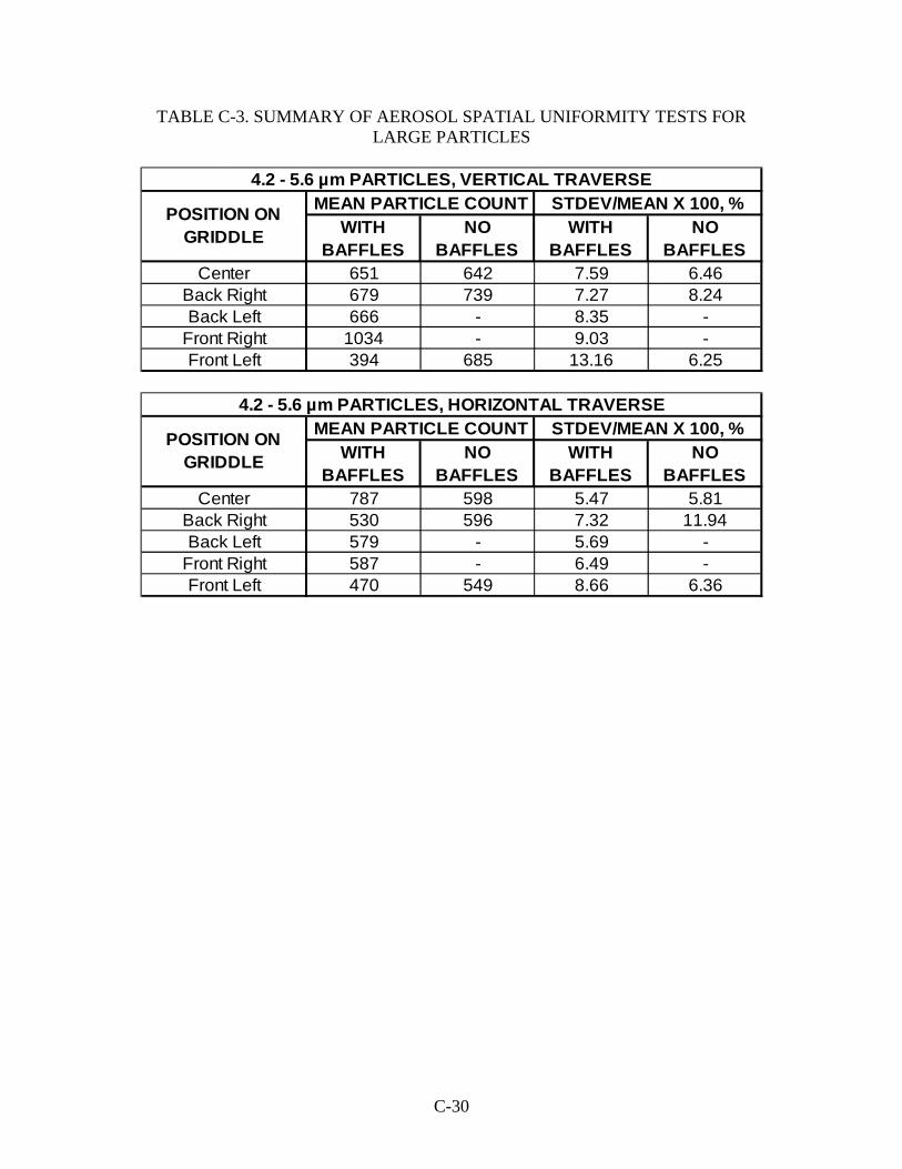
C-30

TABLE C-3. SUMMARY OF AEROSOL SPATIAL UNIFORMITY TESTS FOR LARGE PARTICLES

WITH BAFFLES

NO BAFFLES

WITH BAFFLES

NO BAFFLES

651 642 7.59 6.46679 739 7.27 8.24666 - 8.35 -

1034 - 9.03 -394 685 13.16 6.25

POSITION ON GRIDDLE

MEAN PARTICLE COUNT STDEV/MEAN X 100, %4.2 - 5.6 µm PARTICLES, VERTICAL TRAVERSE

Front Left


Front Right

WITH BAFFLES

NO BAFFLES

WITH BAFFLES

NO BAFFLES

787 598 5.47 5.81530 596 7.32 11.94579 - 5.69 -587 - 6.49 -470 549 8.66 6.36

POSITION ON GRIDDLE

MEAN PARTICLE COUNT STDEV/MEAN X 100, %4.2 - 5.6 µm PARTICLES, HORIZONTAL TRAVERSE

Front Left


Front Right

D-1

APPENDIX D

GRIDDLE CALIBRATION PROCEDURES

D-2

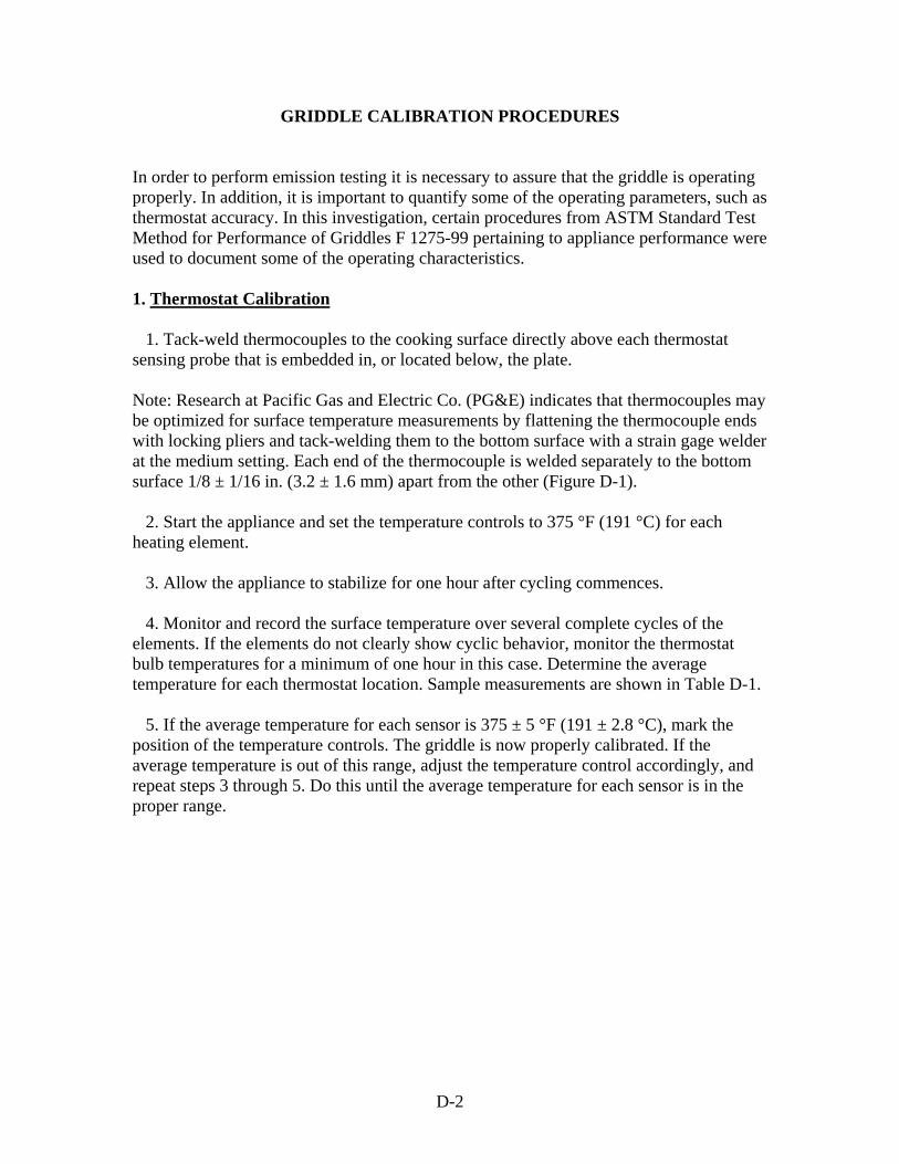
GRIDDLE CALIBRATION PROCEDURES

In order to perform emission testing it is necessary to assure that the griddle is operating properly. In addition, it is important to quantify some of the operating parameters, such as thermostat accuracy. In this investigation, certain procedures from ASTM Standard Test Method for Performance of Griddles F 1275-99 pertaining to appliance performance were used to document some of the operating characteristics. 1. Thermostat Calibration

1. Tack-weld thermocouples to the cooking surface directly above each thermostat sensing probe that is embedded in, or located below, the plate. Note: Research at Pacific Gas and Electric Co. (PG&E) indicates that thermocouples may be optimized for surface temperature measurements by flattening the thermocouple ends with locking pliers and tack-welding them to the bottom surface with a strain gage welder at the medium setting. Each end of the thermocouple is welded separately to the bottom surface 1/8 ± 1/16 in. (3.2 ± 1.6 mm) apart from the other (Figure D-1).

2. Start the appliance and set the temperature controls to 375 °F (191 °C) for each heating element.

3. Allow the appliance to stabilize for one hour after cycling commences.

4. Monitor and record the surface temperature over several complete cycles of the elements. If the elements do not clearly show cyclic behavior, monitor the thermostat bulb temperatures for a minimum of one hour in this case. Determine the average temperature for each thermostat location. Sample measurements are shown in Table D-1.

5. If the average temperature for each sensor is 375 ± 5 °F (191 ± 2.8 °C), mark the position of the temperature controls. The griddle is now properly calibrated. If the average temperature is out of this range, adjust the temperature control accordingly, and repeat steps 3 through 5. Do this until the average temperature for each sensor is in the proper range.

D-3

Figure D-1. Sample of Thermocouple Welding for a 3 by 2 ft (0.9 by 0.6 m) Griddle, from ASTM 1275-99

Table D-1 shows the measured temperatures taken at 5 minute increments on each heating element.

TABLE D-1. TEMPERATURE MEASUREMENTS FOR GRIDDLE CALIBRATION

1, °F 2, °F 3, °F 4, °F 5, °F 6, °F0 388 383 389 391 385 3795 384 382 394 389 383 37210 381 387 370 372 372 38515 366 389 380 381 382 38820 374 361 365 368 379 38625 387 375 384 385 388 37830 376 380 386 364 372 37835 366 382 373 377 374 38940 368 381 388 390 382 37545 382 363 368 368 388 38850 387 370 383 384 372 37355 366 375 390 375 376 38460 367 388 373 375 387 370

Avg. Temp. 376 378 380 378 380 380

Heating ElementTime, min.

E-1

APPENDIX E

PARTICLE COLLECTION EFFICIENCY TEST PROTOCOL

E-2

PARTICLE COLLECTION EFFICIENCY TEST PROTOCOL

A. Particle Collection Efficiency Test Protocol when Cooking Hamburger Note: The cooking procedures used are modeled after the ASTM Standard Test Method for Performance of Griddles, F 1275-99. Efforts were made to duplicate each step of this standard testing procedure, when possible.

1. Position the griddle properly under the exhaust hood. The griddle position is shown in Figure E-1.

2. Calibrate the thermostat settings according to the procedures given in Appendix D.

3. Determine the number of hamburger patties to be cooked for each batch. Follow the guideline given by 10.7.5 from the ASTM test method, for heavy load tests. It was determined that 24 patties, arranged 4 from front to back and 6 from left to right, constituted a heavy load test.

4. Determine the time it takes to cook the hamburgers to 35 % weight loss. The timing

was set up such that patties were sequentially placed on the cooking surface every five seconds for the first two minutes. The patties were allowed to cook for thirty seconds and then flipped at five second intervals. Immediately after the final patty was flipped, the first patty was removed at the same five second interval. Note that the patties must be flipped and removed in the same order that they were loaded. Record the procedure used.

5. Prepare enough food product for the run. Patties are placed on sheet pans 18 x 26 x

1 in. (45.7 x 66 x 2.5 cm), one batch (24 patties) per sheet, on two levels. Each level has twelve patties and is separated by a sheet of wax paper. Weigh two patties from each batch and record the total weight from all batches. It is important to keep track of which patties were weighed in each batch. Place these pans in the freezer until testing.

6. Prepare the appropriate sampling equipment according to appendix F. 7. Set exhaust and makeup air fans to correct frequency for 1000 CFM flow rate.

8. Start the appliance and ventilation system at least one hour before cooking. This

allows the appliance to stabilize. Set the thermostat to 375 °F (191 °C).

9. After the warm-up is complete, check and record the griddle surface temperature. 10. Take an OPC sample to determine background levels.

E-3

11. Bring out the food product. Record the food product temperature immediately before testing begins. It should be 0 ± 5 °F (-17.8 ± 2.8 °C).

12. Start all sampling equipment at the start of the test.

13. Load the hamburger patties sequentially onto the griddle surface. Use the procedure

for 35% weight loss.

14. Turn the hamburger patties sequentially after the given amount of time.

15. Unload the hamburger patties sequentially onto a drip tray after the appropriate time.

16. Turn off sampling equipment after cooking is complete.

17. Scrape the griddle surface and wait for the appliance to re-heat to the proper

temperature (when it resumes cycling). Also, monitor the particle counts until they have reached less than 1 % of their peak test value. Record the elapsed time between the previous load and new load.

18. Repeat steps 9 through 15 for the next test run.

19. Separate the hamburger patties that are to be weighed. Turn the patties in the drip

tray after one minute. Weigh the patties after an additional minute. Determine the weight loss percentage. It should be 35 ± 2 %.

Note 1: Sample time per run: 7 minutes. Note 2: Time to complete collection efficiency test in triplicate: approximately 8-9 hrs. (4 runs without filters and 3 runs with filters). It takes about 1 hour between tests for background levels of OPC 0.32-0.42 channel to reduce to 1% of levels while cooking). B. Particle Collection Efficiency Test Protocol Using Artificial Aerosol Generator

1. Set exhaust and makeup air fans to correct frequency for 1000 CFM flow rate. 2. Turn on griddle to stabilize for one hour after cycling commences (for tests with

griddle on).

3. Turn on OPC and sample background aerosol for 2 minutes.

4. Place large particle aerosol generator outlet in center of griddle and turn on (solution 2:1 oleic acid to isopropyl alcohol).

5. Allow aerosol to stabilize for 5 minutes.

E-4

6. Sample aerosol in exhaust duct for 2 minutes.

7. Insert filters.

8. Set exhaust fan frequency to correct setting for flow rate of 1000 CFM.

9. Allow 2-3 minutes to stabilize.

10. Sample aerosol for 2 minutes.

11. Repeat process for 6 runs without and 5 runs with filters in hood. Note 1: If aerosol is not stable (i.e., OPC 0.32-0.42 channel is not within 2 % of previous run) then repeat run. Note 2: Time to complete collection efficiency test: approximately 2-3 hrs.

E-5

F-1

APPENDIX F

INSTRUMENTATION CALIBRATION AND SAMPLING PROCEDURES

F-2

INSTRUMENTATION CALIBRATION AND SAMPLING PROCEDURES

A. EPA Method 5 1. Clean all glass impinger pieces and sampling probe lines thoroughly of all particles, grease, and sealant. 2. Weigh and record the clean impinger bottles. 3. Fill impingers 2 and 3 with approximately 100 ml (3.4 fl. oz.) DI water, weigh and

record. 4. Fill impinger 4 with approximately 200 g (0.44 lb.) of desiccated silica gel, weigh and

record. 5. Assemble impinger train as follows:

A. Place a small amount of vacuum grease on the ground glass area of the impinger stem. Spread it evenly across the surface.

B. Insert impinger stem into each impinger, twisting the stem back and forth until a good seal is obtained (when you can no longer see streaks from the vacuum grease).

C. Place impingers in the impinger holder. Impinger 1 must be near the front of the holder (where the holding slots are located), while impinger 4 must be near the side of the holder where the gas sample line attaches.

D. Lightly apply vacuum grease to the two ground glass surfaces of each impinger stem.

E. Place and clamp the remaining fittings (three 180° glass elbows, one glass connector to the filter holder, and the stainless steel connector to the large sampling pump unit) on the sample train. The connector to the filter holder must connect to the center (inlet) of impinger 1. The 180° elbows connect from the sides (outlets) of the lower number impingers to the center (inlets) of the next highest number impinger. Connect the stainless steel piece to the outlet of impinger 4.

G. Cover the inlet and outlet to prevent contamination. 6. Place the impinger holder onto the EPA Method 5 sampler by aligning the holding

slots. Fill with ice. 7. Assemble the large glass filter holder and place in the sampler oven. Grease the fittings

and connect the inlet to the sample probe and the outlet to the impinger train. Close the oven.

8. Check for leaks by blocking off the inlet nozzle and reading the pressure gauge on the

EPA sampler. Record the flow rate at 25 in. Hg vacuum.

F-3

9. Turn on the EPA Method 5 sampling train main power, the probe heater, and the oven heater. The probe heater setting should be 1, the lower oven setting should be 7, and the upper oven setting should be 1.

10. Check the probe and oven temperatures. Assure they reach a range of 140 °F (60 °C)

to 220 °F (104 °C). 11. The flow rate should be calibrated with the flow calibrator attached to the inlet

nozzle. Adjustments are made with the coarse and fine adjustment knobs on the EPA sampler. The flow should be 2 lpm (0.071 cfm). After calibration, turn off the sampler pump and let the pressure release.

12. Connect sampling line to sampling probe. B. Personal Cascade Impactor 1. Desiccate at least 10 Mylar substrates and two PVC after-filters for 24 hours or longer. 2. Assemble the impactor with a dummy filter installed and no substrates. Install in test

location. 3. The impactor should be calibrated with the flow calibrator attached to the inlet nozzle.

Adjustments are done with an adjustment knob on the vacuum line between the pump and the impactor. The flow should be 2.0 LPM (0.071 CFM).

4. Remove and disassemble the impactor. 5. Assure the impactor is clean. Wiping down the surfaces with isopropyl alcohol is

usually sufficient. 6. Reassemble the impactor, placing the desiccated filter and substrates and the proper

stages. Weigh and record each substrate and the filter. Seal inlet and outlet ports until ready for use.

C. Isokinetic Sampling Probe Calibration 1. Prepare two Personal Cascade Impactors using the procedure from Section B. 2. Install one impactor at the outlet end of the sampling probe, and install the other

impactor in the duct at the same axial location as the sampling probe inlet. 3. Run impactors simultaneously while cooking hamburger. 4. Run two tests consisting of three batches of hamburger patties (24 per batch).

F-4

5. Find the penetration of the particles through the probe by dividing mass collected on each impactor stage of the downstream probe by the mass collected on each impactor stage of the upstream probe.

D. Diluter/Optical Particle Counter (OPC) System 1. Place the diluter directly beneath the isokinetic sampling probe and connect the diluter

inlet to the sampling probe bottom outlet. 2. Place the OPC directly beneath the diluter and connect the diluter outlet to the OPC

inlet. Make the connecting tube as short and as straight as possible to avoid particle losses.

3. Connect the OPC to a computer via serial cable and set up a program to automatically

acquire data from the OPC during testing. OPC instruction manuals usually contain relevant information and/or sample programs.

4. Power up the OPC and set sampling time to desired time (7 minutes for cooking tests,

2 minutes for oleic acid tests, or 1 minute for spatial uniformity tests). Also set the particle count to count/CF and the initial delay to 5 seconds.

5. Calibrate diluter to a 50:1 dilution ratio using the diluter adjustment knob and record

dP Aerosol Path and dP Total for future reference. Refer to diluter operations manual for model specific calibration procedures.

E. Micro-Orifice Uniform Deposit Impactor (MOUDI) 1. Cut out at least thirteen 37 mm (1.46 in.) diameter aluminum foil substrates (1 mm,

0.039 in. thickness) and two 37 mm (1.46 in.) after-filters. Place in desiccator for at least 24 hours.

2. Carefully weigh and record the substrates and filters and place them in their respective

holders, ten substrates and one filter for each MOUDI run. 3. Connect the MOUDI inlet to the isokinetic sampling probe side outlet. 4. Connect the MOUDI outlet to the vacuum pump with a ‘T’ fitting and an adjustment

knob somewhere between the MOUDI and the EPA Method 5 adjustment knob. 5. Place “dummy” substrate holders and “dummy” filter in the impactor and adjust the

upper pressure drop to 20.1 in. H2O (0.71 psi), which corresponds to 30 lpm (1.06 CFM).

6. Make sure the lower pressure drop does not exceed 7 psi (193.8 in. H2O). If it does,

clean the last 4 stages of the impactor.

F-5

7. Remove and disassemble the MOUDI. After making sure everything is clean, install substrates and filter.

8. Seal inlet and outlet until testing to prevent substrate contamination. F. Test and Sampling Procedures 1. Position the griddle properly using a tape measure. Record position. 2. Turn on exhaust fan, determining the proper frequency for the flow rate according to

Appendix B. Record the frequency and the centerline velocity (using the anemometer). See that the centerline velocity agrees with the desired flow rate.

3. Make sure all windows and doors are closed. 4. Turn on multimeter and griddle. Pre-heat the griddle at 375 °F (191 °C) (calibrated

according to Appendix D) for one hour. 5. Place the sample probe inlets in their proper in duct positions using a tape measure and

record. Make sure probes are secured and nozzles are facing exactly parallel to exhaust flow.

6. Attach previously assembled and calibrated EPA Method 5 sample train, OPC/Diluter

system, and MOUDI to their respective sample probe (if applicable for particular test).

7. Turn on the EPA Method 5 sampling train main power (if used for test), the probe

heater, and the oven heater. Check the probe and oven temperatures. Assure they are at the correct settings and in the range of 140 to 220 °F (60 to 104 °C).

8. Turn on the OPC and the computer. Make sure all settings are correct, and set a path

and filename on the computer for the collected test run data. 9. Take a sample with the OPC to determine background levels. 10. Determine and record the following: A. Room temperature B. Room barometric pressure C. Room humidity D. Room conditions (doors, windows, AHU) E. Volumetric flow reading on the EPA sampler (if applicable). 11. Prepare for particular test using specified protocol from Appendix E. 12. Remove the covers from the control substrate and filter and place in a location that is

open to the air.

F-6

13. Close the kitchen door and prepare for testing. 14. Periodically check the upper and lower pressure drops of the MOUDI. If the upper

pressure drop changes, adjust it back to 20.1 in. H2O (0.71 psi). Simply record the lower pressure drop.

15. Record the following during testing: A. Cooking times (if applicable) 1. Time to put product on (once for each batch) 2. Time to turn product (once for each batch) 3. Time to remove product (once for each batch) 4. Time between batches 5. Cooking time on each side 6. Total sampling time B. Temperatures (taken at beginning, middle and end of test, if applicable, unless

noted otherwise) 1. Oven 2. Stack 3. Probe 4. Impinger outlet 5. Ambient air 6. Sampling Location 7. Hood 8. Griddle (taken once at beginning and once at end of test) 16. Terminate sampling by turning off the pumps. The OPC should automatically stop at

the set time. 17. Repeat procedure for subsequent tests. 18. After all testing has been completed, turn off appliance, and all pumps and heaters.

Perform a preliminary clean-up, and turn off ventilation hood when appliance cools. If test was not a cooking test, then skip to step 24. 19. Weigh and record hamburgers that were pre-weighed before cooking. Determine the

weight loss and thus doneness. Discard these patties. 20. Remove and disassemble the Personal Cascade Impactor (if applicable). Weigh and

record each substrate and filter. 21. Remove and disassemble the MOUDI. Weigh and record each substrate and filter. 22. Thoroughly clean the impactors. Clean the metal surfaces with isopropyl alcohol.

Rinse with DI water and blow dry. Clean o-rings, when necessary, with DI water.

F-7

23. Weigh and record 8 clean 150 ml glass beakers. Repeat 3 times for each, being sure to

discharge all static charges. Use the average weight for calculations. 24. Weigh the inlet probe. Wash out the inlet probe with acetone and collect in beaker 7. 25. Remove and disassemble the impinger train. Remove vacuum grease from all

surfaces during disassembly. 26. Weigh and record each impinger. 27. Empty water from impingers 2 and 3 into beakers 1 and 2 respectively. Fill beaker 3

(control beaker) with approximately the same amount of DI water. 28. Empty the silica get into a dish and place in the drying oven. 29. Wash all inside surfaces of impingers 1, 2, and 3 with acetone, and collect the acetone

in beakers 4, 5, and 6, respectively.

30. Determine whether beaker 4, 5, 6, or 7 has the most acetone and fill the others to an equal amount. Then, fill beaker 8 (control beaker) with an equal amount of acetone. All of the acetone should come from the same source.

31. Place all 8 beakers under the evaporating hood. 32. Rinse all impinger glassware with water, scrubbing off any obvious vacuum grease

and place in an ultrasonic cleaning bath. Clean for 20 to 30 minutes. Rinse with DI water and place in drying oven. When dry, reassemble impinger train without vacuum grease, and cover inlet and outlet with tape to avoid contamination.

33. Cover inlet and outlet of long sample probe to prevent contamination. 34. Weigh and record beakers 1 through 8 after evaporation has occurred. 35. Enter all data into the spreadsheet. 36. Thoroughly clean the appliance.

G-1

APPENDIX G

ANALYTIC PROCEDURES

G-2

ANALYTIC PROCEDURES

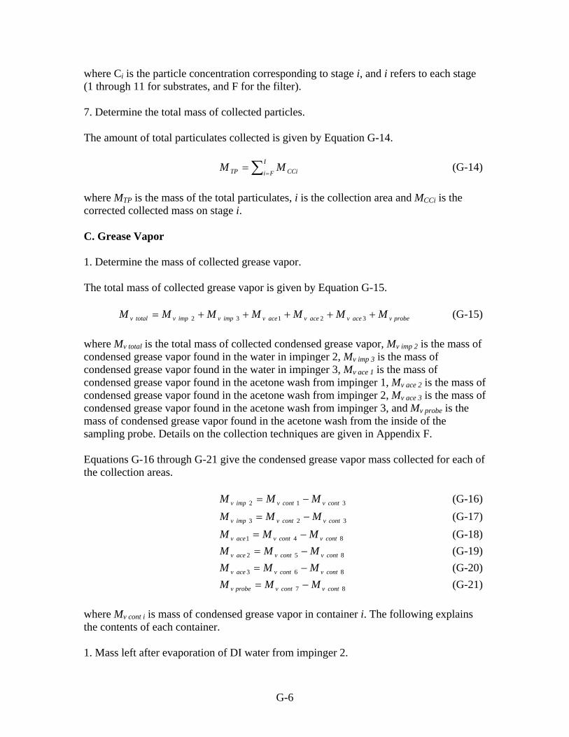
A. Particle Size Distribution from the Personal Cascade Impactor 1. Find the mass of grease collected on each impaction stage and the filter by determining the difference in mass before and after sample collection. Equation G-1 gives the mass of grease collected. BiAiCi MMM -= (G-1) where MC is the mass of grease collected on each stage, MA is the mass of each substrate or filter after sampling, MB is the mass of each substrate or filter before sampling, and i is each substrate or filter position (1 through 8 for substrates, and F for the filter). 2. Find the mass of collected particulates on the control substrate and filter by determining the difference in mass before and after sample collection. Equation G-2 gives the mass of collected particulates on the control substrate and filter. substratecontrolBsubstratecontrolAsubstratecontrol MMM -= (G-2) filtercontrolBfiltercontrolAiltercontrol MMM f -= where Mcontrol substrate is the mass collected on the control substrate, Mcontrol filter is the mass collected on the control filter, MB and MA are the mass before and after sample collection, respectively, for either the control substrate or filter. 3. Find the corrected mass collected by subtracting the mass collected on the control substrate (or filter) from each test substrate (or filter) stage. Equation G-3 gives the corrected mass collected for each stage. substratecontrolCicCi MMM −= (G-3) filtercontrolCFcCF MMM −= where McCi is the corrected mass collected on each stage, McCF is the corrected mass collected for the filter, and i is for substrate positions 1 through 8. 4. Find the particle losses for impaction stages. Surfaces other than impaction plates within the inertial impactor that collect particles must be considered. Rubow et. al. (1987) evaluated the Marple impactor for internal losses as a function of particle size. The main source of particle loss to the probe would be due to sampling efficiency. However, near isokinetic conditions exist at the probe inlet, and these losses are minimized. Table G-1 shows the cut size, dp50, of each stage, and the percentage of particles lost for impaction stages 1 through 8 and the filter.

G-3

TABLE G-1. PERSONAL CASCADE IMPACTOR INTERNAL LOSSES

Stage dp50 µm (in.)

CF (Particle losses) %

1 21.3 (8.4 x 10-4) 24 2 14.8 (5.8 x 10-4) 13 3 9.8 (3.9 x 10-4) 8 4 6.0 (2.4 x 10-4) 7 5 3.5 (1.4 x 10-4) 5 6 1.55 (6.10 x 10-5) 3.5 7 0.93 (3.7 x 10-5) 3 8 0.52 (2.0 x 10-5) 0.5 F 0.01 (3.9 x 10-7) 0

Equation G-4 gives the corrected collected mass for each of the impaction stages.

( )CFM

M cCiCCi −

=1

(G-4)

where MCCi is the corrected collected mass on stage i, and CF is the correction factor given in Table G-1. Note, for the mass collected on the filter, MCF, the corrected collected mass is determined by using a value of 0 for CF. 5. Determine the volume of gas sampled. The volume of gas sampled is given by Equation G-5. ss tQV ⋅= (G-5) where Vs is the air sample volume, Q is the air sampling flow rate, and ts is the total sampling time. 6. Find the particle concentration. The particle concentration is given by Equation G-6.

s

CCii V

MC = (G-6)

where Ci is the particle concentration corresponding to stage i, and i refers to each stage (1 through 8 for substrates, and F for the filter). 7. Determine the total mass of collected particles. The amount of total particulates collected is given by Equation G-7.

G-4

∑=

=1

Fi CCiTP MM (G-7) where MTP is the mass of the total particulates, i is the collection area and MCCi is the corrected collected mass on stage i. B. Particle Size Distribution from the MOUDI 1. Find the mass of grease collected on each impaction stage and the filter by determining the difference in mass before and after sample collection. Equation G-8 gives the mass of grease collected. BiAiCi MMM -= (G-8) where MC is the mass of grease collected on each stage, MA is the mass of each substrate or filter after sampling, MB is the mass of each substrate or filter before sampling, and i is each substrate, or filter position (1 through 11 for substrates, F for the filter). 2. Find the mass of collected particulates on the control substrate and filter by determining the difference in mass before and after sample collection. Equation G-9 gives the mass of collected particulates on the control substrate and filter. substratecontrolBsubstratecontrolAsubstratecontrol MMM -= (G-9) filtercontrolBfiltercontrolAiltercontrol MMM f -= where Mcontrol substrate is the mass collected on the control substrate, Mcontrol filter is the mass collected on the control filter, MB and MA are the mass before and after sample collection, respectively, for either the control substrate or filter. 3. Find the corrected mass collected by subtracting the mass collected on the control substrate (or filter) from each test substrate (or filter) stage. Equation G-10 gives the corrected mass collected for each stage. substratecontrolCicCi MMM −= (G-10) filtercontrolCFcCF MMM −= where McCi is the corrected mass collected on each stage, McCF is the corrected mass collected for the filter, and i is for substrate positions 1 through 11. 4. Find the particle losses for impaction stages. Surfaces other than impaction plates within the inertial impactor that collect particles must be considered. Marple et. al. (1991) evaluated the MOUDI for internal losses as a

G-5

function of particle size. Table G-2 shows the cut size, dp50, of each stage, and the percentage of particles lost for impaction stages 1 through 11 and the filter.

TABLE G-2. MOUDI INTERNAL LOSSES

Stage Dp50

µm (in.) CF (Particle losses)

% 1 18 (7.1 x 10-4) 33 2 10.0 (3.9 x 10-4) 20 3 5.6 (2.2 x 10-4) 9 4 3.2 (1.3 x 10-4) 2.5 5 1.8 (7.1 x 10-5) 1 6 1.00 (3.94 x 10-5) 1 7 0.56 (2.2 x 10-5) 1 8 0.32 (1.3 x 10-5) 1 9 0.18 (7.1 x 10-6) 1 10 0.100 (3.9 x 10-6) 3 11 0.056 (2.2 x 10-6) 8 F 0.01 (3.9 x 10-7) 0

Equation G-11 gives the corrected collected mass for each of the impaction stages.

( )CFM

M cCiCCi −

=1

(G-11)

where MCCi is the corrected collected mass on stage i, and CF is the correction factor given in Table G-2. Note, for the mass collected on the filter, MCF, the corrected collected mass is determined by using a value of 0 for CF. 5. Determine the volume of gas sampled. The volume of gas sampled is given by Equation G-12. ss tQV ⋅= (G-12) where Vs is the air sample volume, Q is the air sampling flow rate, and ts is the total sampling time. 6. Find the particle concentration. The particle concentration is given by Equation G-13.

s

CCii V

MC = (G-13)

G-6

where Ci is the particle concentration corresponding to stage i, and i refers to each stage (1 through 11 for substrates, and F for the filter). 7. Determine the total mass of collected particles. The amount of total particulates collected is given by Equation G-14. ∑=

=I

Fi CCiTP MM (G-14) where MTP is the mass of the total particulates, i is the collection area and MCCi is the corrected collected mass on stage i. C. Grease Vapor 1. Determine the mass of collected grease vapor. The total mass of collected grease vapor is given by Equation G-15. probevacevacevacevimpvimpvtotalv MMMMMMM 3 2 1 3 2 +++++= (G-15) where Mv total is the total mass of collected condensed grease vapor, Mv imp 2 is the mass of condensed grease vapor found in the water in impinger 2, Mv imp 3 is the mass of condensed grease vapor found in the water in impinger 3, Mv ace 1 is the mass of condensed grease vapor found in the acetone wash from impinger 1, Mv ace 2 is the mass of condensed grease vapor found in the acetone wash from impinger 2, Mv ace 3 is the mass of condensed grease vapor found in the acetone wash from impinger 3, and Mv probe is the mass of condensed grease vapor found in the acetone wash from the inside of the sampling probe. Details on the collection techniques are given in Appendix F. Equations G-16 through G-21 give the condensed grease vapor mass collected for each of the collection areas. 3 1 2 contvcontvimpv MMM −= (G-16) 3 2 3 contvcontvimpv MMM −= (G-17) 8 4 1 contvcontvacev MMM −= (G-18) 8 5 2 contvcontvacev MMM −= (G-19) 8 6 3 contvcontvacev MMM −= (G-20) 8 7 contvcontvprobev MMM −= (G-21) where Mv cont i is mass of condensed grease vapor in container i. The following explains the contents of each container. 1. Mass left after evaporation of DI water from impinger 2.

G-7

2. Mass left after evaporation of DI water from impinger 3. 3. Mass left after evaporation of DI water blank. 4. Mass left after evaporation of acetone wash from impinger 1. 5. Mass left after evaporation of acetone wash from impinger 2. 6. Mass left after evaporation of acetone wash from impinger 3. 7. Mass left after evaporation of acetone wash from sampling probe. 8. Mass left after evaporation of the acetone blank. The blanks are used to account for any residue that might be in the DI water or acetone, and any particulates that may fall in the containers during evaporation in the evaporation hood. Details are given in Appendix F. The mass left in the containers after evaporation is determined by Equation G-22. icontBicontAicontv MMM −= (G-22) where icontAM is the average mass of container i after evaporation, and icontBM is the average mass of container i before sample collection. It is important that care is taken in dissipating all static charge before weighing the glass containers. At least three weightings are recommended to determine the average weights. 2. Determine the volume of gas sampled. The volume of gas sampled is given by Equation G-23. ss tQV ⋅= (G-23) where Vs is the air sample volume, Q is the air sampling flow rate, and ts is the total sampling time. 3. Find the particle concentration. The particle concentration is given by Equation G-24.

s

totalv

VM

C = (G-24)

where C is the particle concentration. D. Determination of Particle Collection Efficiency Note: The following procedures are modeled after ANSI/ASHRAE Standard 52.2-99. Efforts were made to duplicate each step of the analytic procedures, when possible. The efficiency calculations are performed separately for each of the OPC size ranges.

G-8

1. Penetration calculations

The penetration is the fraction of particles that pass through the air cleaner. The tests should be performed at a flow rate of 1000 CFM with either the particle generator on, or with cooking taking place. The general equation for the penetration is

installed device(s)t test ion withouconcentrat particleinstalled device(s)est ion with tconcentrat particle

=P

where P is the penetration. Each test consists of three runs, a run without filters, a run with filters, and another run without filters. The average of the two without filter counts should be taken to obtain an estimate of the without filter count that would have occurred at the same time as the count with filters.

2

,),1(,,,,

toitoitei

WOWOWO ++

= (G-25)

where WOi,e,t is the estimated count without filters, WOi,o,t is the first without filter count, and WO(i+1),o,t is the second without filter count, taken after the count with filters. Simply average the background counts from before and after the aerosol generation test by using the following equations:

n

WOWO ni

boi

b

∑→== 1

,,

(G-26)

n

WW ni

boi

b

∑→== 1

,,

where bWO is the average of the background counts without filters, and bW is the average of the background counts with filters. Calculate the observed penetration for each with and without filter sample set using the observed count with filters, the count without filters, the average background count with filters, the average background count without filters, the sampling time without filters, and the sampling time with filters.

⎟⎟⎠

⎞⎜⎜⎝

⎛≤⋅

−

−=

∑→=

wo

wniuoi

uclb

w

wo

btei

btoioi T

Tn

WOW

TT

WOWOWW

P 1,,

,

,,

,,, 05.0 if (G-27a)

G-9

⎟⎟⎠

⎞⎜⎜⎝

⎛>⋅=

∑→=

wo

wniuoi

uclb

w

wo

tei

toioi T

Tn

WOW

TT

WOW

P 1,,

,

,,

,,, 05.0 if (G-27b)

where Pi,o is the observed penetration, Two is the sampling time without filters, and Tw is the sampling time with filters. The observed penetrations should be simply averaged to determine an average observed penetration value.

n

PP ni

oi

o

∑→== 1

,

(G-28)

where oP is the average observed penetration value, and n is the number of samples. The standard deviation of the observed penetration can be calculated as follows:

1

)(1

2,

−

−=

∑→=

n

PPni

ooi

tδ (G-29)

where δt is the standard deviation of the observed penetration. Find the standard deviation of the background counts with and without filters using the following equations:

1

)( 2

1,,

, −

−=

∑→=

n

WOWOni

bboi

bwoδ (G-30)

1

)( 2

1,,

, −

−=

∑→=

n

WWni

bboi

bwδ

where δwo,b is the standard deviation of the background counts without filters, and δw,b is the standard deviation of the background counts with filters.

G-10

TABLE G-3. t DISTRIBUTION VARIABLE

Number of Samples, n

Degrees of Freedom, v = n – 1

t

3 2 4.303 4 3 3.182 5 4 2.776 6 5 2.571 7 6 2.447 8 7 2.365 9 8 2.306 10 9 2.262 11 10 2.228 12 11 2.201 13 12 2.179 14 13 2.160 15 14 2.145 16 15 2.131 17 16 2.120 18 17 2.110 19 18 2.101 20 19 2.093 21 20 2.086 22 21 2.080 23 22 2.074 24 23 2.069 25 24 2.064 26 25 2.060 27 26 2.056 28 27 2.052 29 28 2.048 30 29 2.045 inf. inf. 1.960

The 95 % confidence limits of the penetration are determined by

ntPP tolcl ⋅−= δ (G-31)

ntPP toucl ⋅+= δ (G-32)

where lclP and uclP are the lower and upper confidence limits, respectively, of the final penetration, and t is found by using the t distribution chart, Table G-3, for a given n.

G-11

The 95 % upper confidence limits of the background counts are determined by

ntWOWO bwobuclb ⋅+= , , δ (G-33)

ntWW bwbuclb ⋅+= , , δ (G-34)

where uclbWO , and uclbW , are the 95 % upper confidence limits of the background counts with and without filters, respectively, and t is found by using the t distribution chart, Table G-3, for a given n. There should be at least three sample runs for the penetration to be accurate, and the penetration error limit is as follows:

8-1 numbers channelfor greater, is whichever0.05,or 07.0 ≤⋅≤⋅ ot Pntδ (G-35a)

10 and 9 numbers channelfor greater, is whichever0.05,or 15.0 ≤⋅≤⋅ ot Pntδ (G-35b)

12 and 11 numbers channelfor greater, is whichever0.05,or 20.0 ≤⋅≤⋅ ot Pntδ (G-35c)

where the channel number and corresponding OPC size ranges are given in Table G-4. This requirement should be satisfied before moving on to subsequent sample sets. If the above condition cannot be met, the upper confidence limit for penetration, uclP , shall be used to calculate efficiency for that size range. The 95% upper confidence limit of the background counts with and without the filter should be less than 1 % of the average estimated count when cooking.

100

, 1,,

,,⋅

<∑→=

n

WOWOW ni

tei

uclbuclb (G-36)

Note that there are no background constraints when using the aerosol generator. The sum of the estimated counts without a test device should be at least 500 in each of the particle size channels. If sufficient numbers of counts are not obtained, the sampling time or aerosol generation rate should be increased.

∑→=

≥ni

teiWO1

,, 500 (G-37)

G-12

TABLE G-4. CHANNEL NUMBERS AND OPC SIZE RANGES

1 0.32-0.422 0.42-0.563 0.56-0.754 0.75-1.05 1.0-1.36 1.3-1.87 1.8-2.48 2.4-3.29 3.2-4.210 4.2-5.611 5.6-7.512 7.5-10.013 10.0-13.014 13.0-18.0

Channel Number

Particle Size Range, µm

2. Particle collection efficiency calculations The collection efficiency is the fraction of particles that are captured in the air cleaner. The general equation is

100installed device(s)t test ion withouconcentrat particle

installed device(s)est ion with tconcentrat particle1efficiency collection ×⎟⎟⎠

⎞⎜⎜⎝

⎛−=

100)1( ×−= oP (G-38) where oP is the average observed penetration.

H-1

APPENDIX H

UNCERTAINTY ANALYSIS

H-2

UNCERTAINTY ANALYSIS

A. Particle Size Distribution from the Personal Cascade Impactor 1. Find the uncertainty associated with the mass of grease collected on each impaction stage and the filter. Equation G-1 is used to find the mass on each impaction stage. Equation G-1 involves the subtraction of two masses; therefore, Equation H-1 gives the absolute uncertainty associated with each mass.

( ) ( )22BiAiCi MMM ∆+∆=∆ (H-1)

The values for ∆MAi and ∆MBi are determined by the accuracy and precision of the scale used to obtain the masses. ∆MAi or Bi is estimated to be ± 0.005 mg (2.3 x 10-9 lb). 2. Find the uncertainty in the corrected collected particulate mass, MCCi. Uncertainties associated with the correction factor, CF, used to correct the collected mass on stages 1 through 8, must be determined. Equation G-4 gives the corrected collected mass, MCCi. It is necessary to calculate the absolute uncertainty in MCCi, because the collected mass could equal 0. Therefore, the relative uncertainty would be indeterminant. However, even if MCi and hence MCCi are 0, uncertainties still exist. If we consider the quotient, (1-CF), to be the one term (as opposed to considering CF independently) Equation H-2 gives the absolute uncertainty of MCCi.

2

2

2

)1()1(

)1(1

⎥⎦

⎤⎢⎣

⎡⎟⎟⎠

⎞⎜⎜⎝

⎛−−

−∆+⎥⎦

⎤⎢⎣

⎡⎟⎟⎠

⎞⎜⎜⎝

⎛−

∆=∆CFM

CFCF

MM cCicCiCCi (H-2)

The absolute uncertainty in (1-CF) is determined by estimating the error associated with the graph from which the values of CF, for each impaction stage, were read. Note, for the filter and the combined mass collection areas, CF is 0, therefore, ∆McCF is equal to ∆MCCF. 3. Find the uncertainty associated with the total mass. Equation G-7 gives the mass of the total particulates, MTP. It is simply the addition of all the corrected collected masses. Equation H-3 gives the absolute uncertainty in MTP.

( )∑=

∆=∆1

2

FiCCiTP MM (H-3)

H-3

B. Particle Size Distribution from the MOUDI 1. Find the uncertainty associated with the mass of grease collected on each impaction stage and the filter. Equation G-8 is used to find the mass on each impaction stage. Equation G-8 involves the subtraction of two masses; therefore, Equation H-4 gives the absolute uncertainty associated with each mass.

( ) ( )22BiAiCi MMM ∆+∆=∆ (H-4)

The values for ∆MAi and ∆MBi are determined by the accuracy and precision of the scale used to obtain the masses. ∆MAi or Bi is estimated to be ± 0.005 mg (2.3 x 10-9 lb). 2. Find the uncertainty in the corrected collected particulate mass, MCCi. Uncertainties associated with the correction factor, CF, used to correct the collected mass on stages 1 through 11, must be determined. Equation G-11 gives the corrected collected mass, MCCi. It is necessary to calculate the absolute uncertainty in MCCi, because the collected mass could equal 0. Therefore, the relative uncertainty would be indeterminant. However, even if MCi and hence MCCi are 0, uncertainties still exist. If we consider the quotient, (1-CF), to be the one term (as opposed to considering CF independently) Equation H-5 gives the absolute uncertainty of MCCi.

2

2

2

)1()1(

)1(1

⎥⎦

⎤⎢⎣

⎡⎟⎟⎠

⎞⎜⎜⎝

⎛−−

−∆+⎥⎦

⎤⎢⎣

⎡⎟⎟⎠

⎞⎜⎜⎝

⎛−

∆=∆CFM

CFCF

MM cCicCiCCi (H-5)

The absolute uncertainty in (1-CF) is determined by estimating the error associated with the graph from which the values of CF, for each impaction stage, were read. Note, for the filter and the combined mass collection areas, CF is 0, therefore, ∆McCF is equal to ∆MCCF. 3. Find the uncertainty associated with the total mass. Equation G-14 gives the mass of the total particulates, MTP. It is simply the addition of all the corrected collected masses. Equation H-6 gives the absolute uncertainty in MTP.

( )∑=

∆=∆I

FiCCiTP MM 2 (H-6)

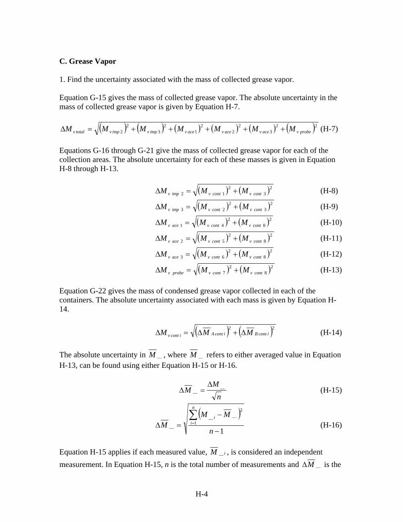
H-4

C. Grease Vapor 1. Find the uncertainty associated with the mass of collected grease vapor. Equation G-15 gives the mass of collected grease vapor. The absolute uncertainty in the mass of collected grease vapor is given by Equation H-7.

( ) ( ) ( ) ( ) ( ) ( )2 2

3 2

2 2

1 2

3 2

2 probevacevacevacevimpvimpvtotalv MMMMMMM +++++=∆ (H-7) Equations G-16 through G-21 give the mass of collected grease vapor for each of the collection areas. The absolute uncertainty for each of these masses is given in Equation H-8 through H-13.

( ) ( )23

21 2 contvcontvimpv MMM +=∆ (H-8)

( ) ( )23

22 3 contvcontvimpv MMM +=∆ (H-9)

( ) ( )28

24 1 contvcontvacev MMM +=∆ (H-10)

( ) ( )28


( ) ( )28


( ) ( )28

27 contvcontvprobev MMM +=∆ (H-13)

Equation G-22 gives the mass of condensed grease vapor collected in each of the containers. The absolute uncertainty associated with each mass is given by Equation H-14.

( ) ( )2 2

icontBicontAicontv MMM ∆+∆=∆ (H-14) The absolute uncertainty in __M , where __M refers to either averaged value in Equation H-13, can be found using either Equation H-15 or H-16.

n

MM __

__∆

=∆ (H-15)

( )

11

2____

__−

−=∆∑=

n

MMM

n

ii

(H-16)

Equation H-15 applies if each measured value, iM __ , is considered an independent measurement. In Equation H-15, n is the total number of measurements and __M∆ is the

H-5

absolute measurement uncertainty associated with each iM __ . Equation H-15 is valid when __M is the same for all measurements, as would apply to a scale. The uncertainty associated with the scale is used for determining __M∆ and was found to be ±0.5 mg (1.1x10-3 lb.). Equation H-16 gives the standard deviation of __M , where iM __ is the value of measurement i.

I-1

APPENDIX I

SAMPLE CALCULATIONS

I-2

SAMPLE CALCULATIONS

A complete set of sample calculations are given for the tests with the Personal Cascade Impactor, MOUDI, EPA Method 5, and the OPC while cooking hamburger and for the OPC while generating oleic acid particulates. The calculations follow the format presented in Appendices G and H. A. Particle Size Distribution from the Personal Cascade Impactor 1. The mass collected on each impactor stage substrate and the filter are determined using Equation G-1. Table I-1 shows the mass of the impactor stages before and after collection as well as the net mass collected.

TABLE I-1. MASS COLLECTED ON EACH PCI STAGE

Stage i MBi (mg) MAi (mg) MCi (mg) 1 24.680 24.688 0.008 2 24.621 24.624 0.003 3 24.632 24.670 0.038 4 24.377 24.417 0.040 5 24.635 24.690 0.055 6 24.985 25.044 0.059 7 24.754 24.765 0.011 8 24.460 24.525 0.065 F 12.141 12.356 0.215

2. The mass of collected particulates on the control substrate and filter is given by Equation G-2.

mg 000.0771.24771.24 =−=substratecontrolM mg 002.0326.11324.11f −=−=iltercontrolM

3. The mass collected on each stage corrected for the control substrate and filter, McCi, is given by Equation G-3. Table I-2 shows the collected mass, the control substrate and filter mass, and the corrected collected mass.

I-3

TABLE I-2. CORRECTED COLLECTED MASS WITH RESPECT TO CONTROL FILTER AND SUBSTRATE FOR THE PCI

Stage i MCi (mg) Mcontrol substrate or filter (mg) McCi (mg)

1 0.008 0.000 0.008 2 0.003 0.000 0.003 3 0.038 0.000 0.038 4 0.040 0.000 0.040 5 0.055 0.000 0.055 6 0.059 0.000 0.059 7 0.011 0.000 0.011 8 0.065 0.000 0.065 F 0.215 -0.002 0.217

4. The particle losses within the impactor are determined using Table G-1 and Equation G-4. Table I-3 shows the collected mass, the correction factor, and the corrected collected mass for the various impactor stages.

TABLE I-3. COLLECTED MASS, CORRECTION FACTOR, AND CORRECTED

COLLECTED MASS FOR THE VARIOUS PCI STAGES

Stage i McCi (mg) CF (%) MCCi (mg) 1 0.008 24 0.010 2 0.003 13 0.003 3 0.038 8 0.041 4 0.040 7 0.043 5 0.055 5 0.058 6 0.059 3.5 0.061 7 0.011 3 0.011 8 0.065 0.5 0.065 F 0.217 0 0.217

where McCi is the collected mass (corrected from control substrate and filter), CF is the correction factor related to the particle losses (Table G-1), and MCCi is the corrected collected mass. 5. The volume of gas sampled is determined by Equation G-5.

( ) ( ) 3m 0040.0l 0.4min 2lpm 0.2 ==⋅=sV 6. The particle concentration for each cut size is given by Equation G-6. The corrected collected mass for each stage is divided by the volume of air sampled. Table I-4 shows the associated concentration collected for each impactor stage.

I-4

TABLE I-4. PARTICLE CONCENTRATION FOR EACH PCI STAGE

Stage i MCCi (mg) Ci (mg/m3) 1 0.010 2.500 2 0.003 0.750 3 0.041 10.250 4 0.043 10.750 5 0.058 14.500 6 0.061 15.250 7 0.011 2.750 8 0.065 16.250 F 0.217 54.250

7. The total mass collected in the various particle size ranges are determined using Equation G-7. For the total particulates, the corrected collected mass within each size range is summed. Table I-5 shows the corrected collected mass for each size range, and their sum, giving the mass of total particulates collected.

TABLE I-5. TOTAL PARTICULATES COLLECTED FOR THE PCI

Stage i MCCi (mg) 1 0.010 2 0.003 3 0.041 4 0.043 5 0.058 6 0.061 7 0.011 8 0.065 F 0.215

TOTAL PARTICULATES 0.507 B. Particle Size Distribution from the MOUDI 1. The mass collected on each impactor stage substrate and the filter are determined using Equation G-8. Table I-6 shows the mass of the impactor stages before and after collection as well as the net mass collected.

I-5

TABLE I-6. MASS COLLECTED ON EACH MOUDI STAGE

Stage i MBi (mg) MAi (mg) MCi (mg) 1 75.634 75.682 0.048 2 75.935 76.074 0.139 3 75.735 76.913 1.178 4 76.256 79.450 3.194 5 71.065 73.021 1.956 6 70.786 71.815 1.029 7 70.754 71.023 0.269 8 71.034 71.191 0.157 9 70.472 70.831 0.359 10 70.285 70.359 0.074 11 70.260 70.333 0.073 F 101.365 101.392 0.027

2. The mass of collected particulates on the control substrate and filter is given by Equation G-9.

mg 005.0941.70936.70 −=−=substratecontrolM mg 008.0597.92589.92f −=−=iltercontrolM

3. The mass collected on each stage corrected for the control substrate and filter, McCi, is given by Equation G-10. Table I-7 shows the collected mass, the control substrate and filter mass, and the corrected collected mass.

TABLE I-7. CORRECTED COLLECTED MASS WITH RESPECT TO CONTROL FILTER AND SUBSTRATE FOR THE MOUDI

Stage i MCi (mg) Mcontrol substrate or filter (mg) McCi (mg)

1 0.048 -0.005 0.053 2 0.139 -0.005 0.144 3 1.178 -0.005 1.183 4 3.194 -0.005 3.199 5 1.956 -0.005 1.961 6 1.029 -0.005 1.034 7 0.269 -0.005 0.274 8 0.157 -0.005 0.162 9 0.359 -0.005 0.364 10 0.074 -0.005 0.079 11 0.073 -0.005 0.078 F 0.027 -0.008 0.035

I-6

4. The particle losses within the impactor are determined using Table G-2 and Equation G-11. Table I-8 shows the collected mass, the correction factor, and the corrected collected mass for the various impactor stages.

TABLE I-8. COLLECTED MASS, CORRECTION FACTOR, AND CORRECTED

COLLECTED MASS FOR THE VARIOUS MOUDI STAGES

Stage i McCi (mg) CF (%) MCCi (mg) 1 0.053 33 0.079 2 0.144 20 0.180 3 1.183 9 1.300 4 3.199 2.5 3.281 5 1.961 1 1.981 6 1.034 1 1.044 7 0.274 1 0.277 8 0.162 1 0.164 9 0.364 1 0.368 10 0.079 3 0.081 11 0.078 8 0.085 F 0.035 0 0.035

where McCi is the collected mass (corrected from control substrate and filter), CF is the correction factor related to the particle losses, and MCCi is the corrected collected mass. 5. The volume of gas sampled is determined by Equation G-12. 3 runs were conducted at 7 minutes each, therefore the total sampling time is 21 minutes.

( ) ( ) 3m 63.0l 630min 21lpm 30 ==⋅=sV 6. The particle concentration for each cut size is given by Equation G-13. The corrected collected mass for each stage is divided by the volume of air sampled. Table I-9 shows the associated concentration collected for each impactor stage.

I-7

TABLE I-9. PARTICLE CONCENTRATION FOR EACH MOUDI STAGE

Stage i MCCi (mg) Ci (mg/m3) 1 0.079 0.125 2 0.180 0.285 3 1.300 2.063 4 3.281 5.207 5 1.981 3.144 6 1.044 1.657 7 0.277 0.440 8 0.164 0.260 9 0.368 0.584 10 0.081 0.129 11 0.085 0.135 F 0.035 0.056

7. The total mass collected in the various particle size ranges are determined using Equation G-14. For the total particulates, the corrected collected mass within each size range is summed. Table I-10 shows the corrected collected mass for each size range, and their sum, giving the mass of total particulates collected.

TABLE I-10. TOTAL PARTICULATES COLLECTED FOR THE MOUDI

Stage i MCCi (mg) 1 0.079 2 0.180 3 1.300 4 3.281 5 1.981 6 1.044 7 0.277 8 0.164 9 0.368 10 0.081 11 0.085 F 0.035

TOTAL PARTICULATES 8.875

I-8

C. Grease Vapor 1. The mass of collected grease vapor is determined using Equations G-15 through G-22. Equation G-22 is used to calculate the mass of grease vapor collected in each container. Table I-11 shows the measured and average weight of each container, before and after collection and evaporation, and the net mass of grease vapor collected in each container.

TABLE I-11. DETERMINATION OF THE NET MASS COLLECTED IN EACH CONTAINER FOR GREASE VAPOR CALCULATIONS

Con-tainer

Before collection and evaporation After collection and evaporation

Weighing number icontBM Weighing number icontAM (i) 1 (g) 2 (g) 3 (g) Ave.

(g) 1 (g) 2 (g) 3 (g) Ave.

(g) Mv cont i (mg)

1 69.0152 69.0151 69.0151 69.0151 69.0177 69.0176 69.0174 69.0176 2.5 2 63.8973 63.8971 63.8975 63.8973 63.8989 63.8992 63.8992 63.8991 1.8 3 67.1594 67.1594 67.1593 67.1594 67.1608 67.1608 67.1609 67.1608 1.4 4 62.3552 62.3550 62.3551 62.3551 62.3588 62.3588 62.3587 62.3588 3.7 5 67.0133 67.0137 67.0135 67.0135 67.0168 67.0168 67.0167 67.0168 3.3 6 69.7857 69.7862 69.7865 69.7861 69.7898 69.7899 69.7897 69.7898 3.7 7 68.2992 68.2991 68.2992 68.2992 68.3028 68.3034 68.3031 68.3031 3.9 8 68.4819 68.4818 68.4818 68.4818 68.4842 68.4845 68.4842 68.4843 2.5

Equations G-16 through G-21 are used to determine the mass of collected grease vapor in each vapor collection area.

mg 1.14.15.22 =−=impvM mg 4.04.18.13 =−=impvM mg 2.15.27.31 =−=acevM mg 8.05.23.32 =−=acevM mg 2.15.27.33 =−=acevM mg 4.15.29.3 =−=probevM

Equation G-15 is used to calculate the total mass of grease vapor collected.

mg 1.64.12.18.02.14.01.1 =+++++=totalvM 2. The volume of gas sampled is determined by Equation G-23. 3 runs were conducted at 7 minutes each, therefore the total sampling time is 21 minutes.

( ) ( ) 3m 042.0l 42min 21lpm 2 ==⋅=sV

I-9

3. The particle concentration is given by Equation G-24.

33 mmg 2.145

m042.0mg 1.6

==C

D. Determination of Particle Collection Efficiency

1. Particle Collection Efficiency Calculations for Cooking Tests The data for the following calculations are taken from a hamburger cooking test, with baffles as the tested filtration device. Table I-12 shows the raw data from this test.

TABLE I-12. RAW DATA FROM COOKING TEST,

WITH BAFFLES INSTALLED

0.32-0.42 5,120 1,619,020 2,910 1,624,684 6,580 1,492,400 5,115 1,600,731 4,445 1,802,336 4,225 1,774,629 5,285 1,611,341 4,080

0.42-0.56 1,155 662,344 640 639,740 865 527,124 700 546,196 790 595,310 725 541,984 850 469,080 690

0.56-0.75 375 318,684 250 300,287 215 236,897 125 239,241 225 224,679 150 201,476 230 173,956 175

0.75-1.0 360 360,217 190 337,769 125 261,083 170 263,851 155 233,121 90 203,730 130 177,719 150

1.0-1.3 95 166,891 60 157,021 75 121,420 30 120,464 55 105,174 20 91,639 40 80,643 35

1.3-1.8 110 139,957 45 131,973 45 102,066 45 101,300 60 88,299 35 76,690 40 67,426 40

1.8-2.4 100 157,669 20 150,576 25 117,486 20 116,213 25 103,564 30 88,200 45 78,373 25

2.4-3.2 10 38,873 10 36,314 15 29,367 10 29,057 10 27,797 15 22,066 0 19,627 10

3.2-4.2 5 19,177 5 18,473 15 15,401 5 15,254 0 15,589 10 12,243 0 10,779 5

4.2-5.6 0 14,430 0 13,737 0 11,396 0 10,710 5 11,640 0 9,323 0 8,093 0

5.6-7.5 0 7,826 0 7,080 0 6,219 0 5,756 0 6,617 0 4,791 0 4,276 0

7.5-10.0 0 2,353 0 1,940 0 1,871 0 1,526 0 1,989 0 1,327 0 1,379 0

10.0-13.0 0 494 0 366 0 396 5 234 0 404 0 236 0 301 0

13.0-18.0 0 63 0 30 0 37 0 24 0 46 0 21 0 17 0

size range, µm bg

without baffles bg

with baffles bg

without baffles bg

with baffles bg

without baffles bg

with baffles bg

without baffles bg

The background counts, listed as (bg), are the background counts taken right before the proceeding run. Therefore, the background count without the test device installed is the background data immediately before the ‘without baffles’ data section, whereas the background count with the test device installed is the background data immediately before the ‘with baffles’ data section. 1. Penetration calculations The estimated count without baffles that would have theoretically occurred at the same time as the count with baffles is determined from Equation G-25. Table I-13 shows the estimated count without baffles for each particle size range.

I-10

TABLE I-13. ESTIMATED PARTICLE COUNTS

0.32-0.42 1,555,710 1,647,368 1,706,8390.42-0.56 594,734 561,217 532,1950.56-0.75 277,791 230,788 199,3180.75-1.0 310,650 247,102 205,4201.0-1.3 144,156 113,297 92,9091.3-1.8 121,012 95,183 77,8631.8-2.4 137,578 110,525 90,9692.4-3.2 34,120 28,582 23,7123.2-4.2 17,289 15,495 13,1844.2-5.6 12,913 11,518 9,8675.6-7.5 7,023 6,418 5,4477.5-10.0 2,112 1,930 1,684

10.0-13.0 445 400 35313.0-18.0 50 42 32

size range, µm WO 1,e,t WO 2,e,t WO 3,e,t

The average background counts are determined from Equation G-26. Table I-14 shows the average background count for each particle size range.

TABLE I-14. AVERAGE BACKGROUND COUNTS

0.32-0.42 5,850 4,013 5,513 4,670 4,865 4,1530.42-0.56 1,010 670 828 713 820 7080.56-0.75 295 188 220 138 228 1630.75-1.0 243 180 140 130 143 1201.0-1.3 85 45 65 25 48 281.3-1.8 78 45 53 40 50 381.8-2.4 63 20 25 25 35 282.4-3.2 13 10 13 13 5 133.2-4.2 10 5 8 8 0 84.2-5.6 0 0 3 0 3 05.6-7.5 0 0 0 0 0 07.5-10.0 0 0 0 0 0 0

10.0-13.0 0 3 0 3 0 013.0-18.0 0 0 0 0 0 0

size range, µm 1WO 1W 2WO 2W 3WO 3W

The observed penetration is calculated using Equation G-27. Table I-15 shows the observed penetration for each particle size range.

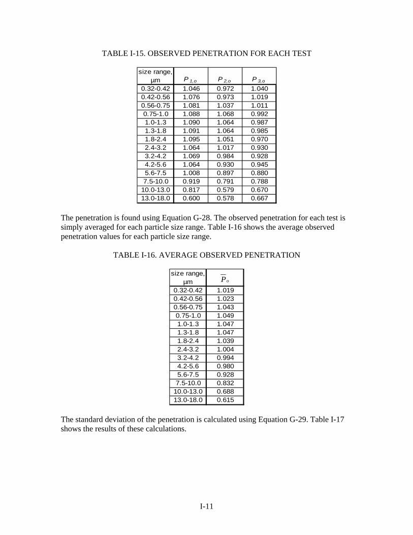
I-11

TABLE I-15. OBSERVED PENETRATION FOR EACH TEST

0.32-0.42 1.046 0.972 1.0400.42-0.56 1.076 0.973 1.0190.56-0.75 1.081 1.037 1.0110.75-1.0 1.088 1.068 0.9921.0-1.3 1.090 1.064 0.9871.3-1.8 1.091 1.064 0.9851.8-2.4 1.095 1.051 0.9702.4-3.2 1.064 1.017 0.9303.2-4.2 1.069 0.984 0.9284.2-5.6 1.064 0.930 0.9455.6-7.5 1.008 0.897 0.8807.5-10.0 0.919 0.791 0.788

10.0-13.0 0.817 0.579 0.67013.0-18.0 0.600 0.578 0.667

size range, µm P 1,o P 2,o P 3,o

The penetration is found using Equation G-28. The observed penetration for each test is simply averaged for each particle size range. Table I-16 shows the average observed penetration values for each particle size range.

TABLE I-16. AVERAGE OBSERVED PENETRATION

0.32-0.42 1.0190.42-0.56 1.0230.56-0.75 1.0430.75-1.0 1.0491.0-1.3 1.0471.3-1.8 1.0471.8-2.4 1.0392.4-3.2 1.0043.2-4.2 0.9944.2-5.6 0.9805.6-7.5 0.9287.5-10.0 0.832

10.0-13.0 0.68813.0-18.0 0.615

size range, µm oP

The standard deviation of the penetration is calculated using Equation G-29. Table I-17 shows the results of these calculations.

I-12

TABLE I-17. STANDARD DEVIATION OF PENETRATION

0.32-0.42 0.0410.42-0.56 0.0520.56-0.75 0.0360.75-1.0 0.0511.0-1.3 0.0541.3-1.8 0.0551.8-2.4 0.0642.4-3.2 0.0683.2-4.2 0.0714.2-5.6 0.0735.6-7.5 0.0707.5-10.0 0.075

10.0-13.0 0.12013.0-18.0 0.046

size range, µm δt

The standard deviation of the background counts are calculated using Equation G-30. Table I-18 shows the results of these calculations.

TABLE I-18. STANDARD DEVIATION OF BACKGROUND COUNTS

0.32-0.42 892.3 905.70.42-0.56 163.2 35.70.56-0.75 76.1 54.00.75-1.0 112.4 43.21.0-1.3 23.9 17.01.3-1.8 32.0 4.81.8-2.4 35.4 4.82.4-3.2 6.3 2.53.2-4.2 7.1 2.54.2-5.6 2.5 0.05.6-7.5 0.0 0.07.5-10.0 0.0 0.0

10.0-13.0 0.0 2.513.0-18.0 0.0 0.0

δwo,b δw,b

size range, µm

The 95% upper and lower confidence limits of the penetration are calculated using Equation G-31 and G-32. Table I-19 shows the values obtained for each particle size range.

I-13

TABLE I-19. 95% CONFIDENCE LIMITS OF THE PENETRATION

0.32-0.42 0.917 1.1210.42-0.56 0.895 1.1510.56-0.75 0.955 1.1320.75-1.0 0.924 1.1751.0-1.3 0.913 1.1801.3-1.8 0.910 1.1841.8-2.4 0.881 1.1972.4-3.2 0.835 1.1733.2-4.2 0.818 1.1704.2-5.6 0.798 1.1625.6-7.5 0.755 1.1027.5-10.0 0.647 1.018

10.0-13.0 0.390 0.98713.0-18.0 0.501 0.729

size range, µm lclP uclP

The 95% upper confidence limits of the background counts are calculated using Equation G-33 and G-34. Table I-20 shows the values obtained for each particle size range.

TABLE I-20. 95% UPPER CONFIDENCE LIMITS OF THE BACKGROUND COUNTS

0.32-0.42 6777.2 5523.50.42-0.56 1174.7 745.50.56-0.75 382.3 260.90.75-1.0 371.4 218.71.0-1.3 104.3 63.31.3-1.8 114.6 48.91.8-2.4 105.1 31.42.4-3.2 18.8 15.23.2-4.2 16.3 10.24.2-5.6 5.2 0.05.6-7.5 0.0 0.07.5-10.0 0.0 0.0

10.0-13.0 0.0 5.213.0-18.0 0.0 0.0

size range, µm uclbWO , uclbW ,

The acceptance criteria for the error limit of the penetration is calculated from Equations G-35a, G-35b, and G-35c. Table I-21 shows the calculations and the corresponding criteria for each particle size range. Note that only the greater of the criteria values have been displayed.

I-14

TABLE I-21. ACCEPTANCE CRITERIA OF THE PENETRATION

0.32-0.42 0.10 0.070.42-0.56 0.13 0.070.56-0.75 0.09 0.070.75-1.0 0.13 0.071.0-1.3 0.13 0.071.3-1.8 0.14 0.071.8-2.4 0.16 0.072.4-3.2 0.17 0.073.2-4.2 0.18 0.154.2-5.6 0.18 0.155.6-7.5 0.17 0.197.5-10.0 0.19 0.17

10.0-13.0 0.3013.0-18.0 0.11

stdev*t/sqrt(n) criteriasize range,

µm

As can be seen from Table I-21, the current test has not passed the acceptance criteria in most particle size ranges. More tests would need to be conducted for the data to be in the required range. The maximum background count criteria are determined using Equation G-36. As shown in Table I-22, the 95 % upper confidence limit of the background counts with and without the filter installed is less than 1 % of the average estimated count for each particle size range.

TABLE I-22. MAXIMUM BACKGROUND COUNT CRITERIA

0.32-0.42 6,777 5,524 16,3660.42-0.56 1,175 746 5,6270.56-0.75 382 261 2,3600.75-1.0 371 219 2,5441.0-1.3 104 63 1,1681.3-1.8 115 49 9801.8-2.4 105 31 1,1302.4-3.2 19 15 2883.2-4.2 16 10 1534.2-5.6 5 0 1145.6-7.5 0 0 63

7.5-10.0 0 0 1910.0-13.0 0 5 413.0-18.0 0 0 0

size range, µm

maximum background

countuclbWO , uclbW ,

I-15

The minimum particle count criteria are determined using Equation G-37. Table I-23 shows the results of these calculations for each particle size range.

TABLE I-23. MINIMUM PARTICLE COUNT CRITERIA

0.32-0.42 4,909,9170.42-0.56 1,688,1460.56-0.75 707,8960.75-1.0 763,1721.0-1.3 350,3611.3-1.8 294,0571.8-2.4 339,0712.4-3.2 86,4143.2-4.2 45,9684.2-5.6 34,2985.6-7.5 18,8877.5-10.0 5,726

10.0-13.0 1,19813.0-18.0 123

size range, µm

particle count

As shown in Table I-23, the minimum particle counts have been satisfied in all size ranges except the 13.0-18.0 µm range. 2. Particle collection efficiency calculations The collection efficiency is calculated using Equation G-38. Table I-24 shows the collection efficiency for each particle size range.

TABLE I-24. COLLECTION EFFICIENCY OF BAFFLES FOR COOKING TEST

0.32-0.42 -1.930.42-0.56 -2.280.56-0.75 -4.320.75-1.0 -4.911.0-1.3 -4.661.3-1.8 -4.681.8-2.4 -3.862.4-3.2 -0.383.2-4.2 0.624.2-5.6 2.035.6-7.5 7.187.5-10.0 16.76

10.0-13.0 31.1613.0-18.0 38.50

size range, µm

collection efficiency, %

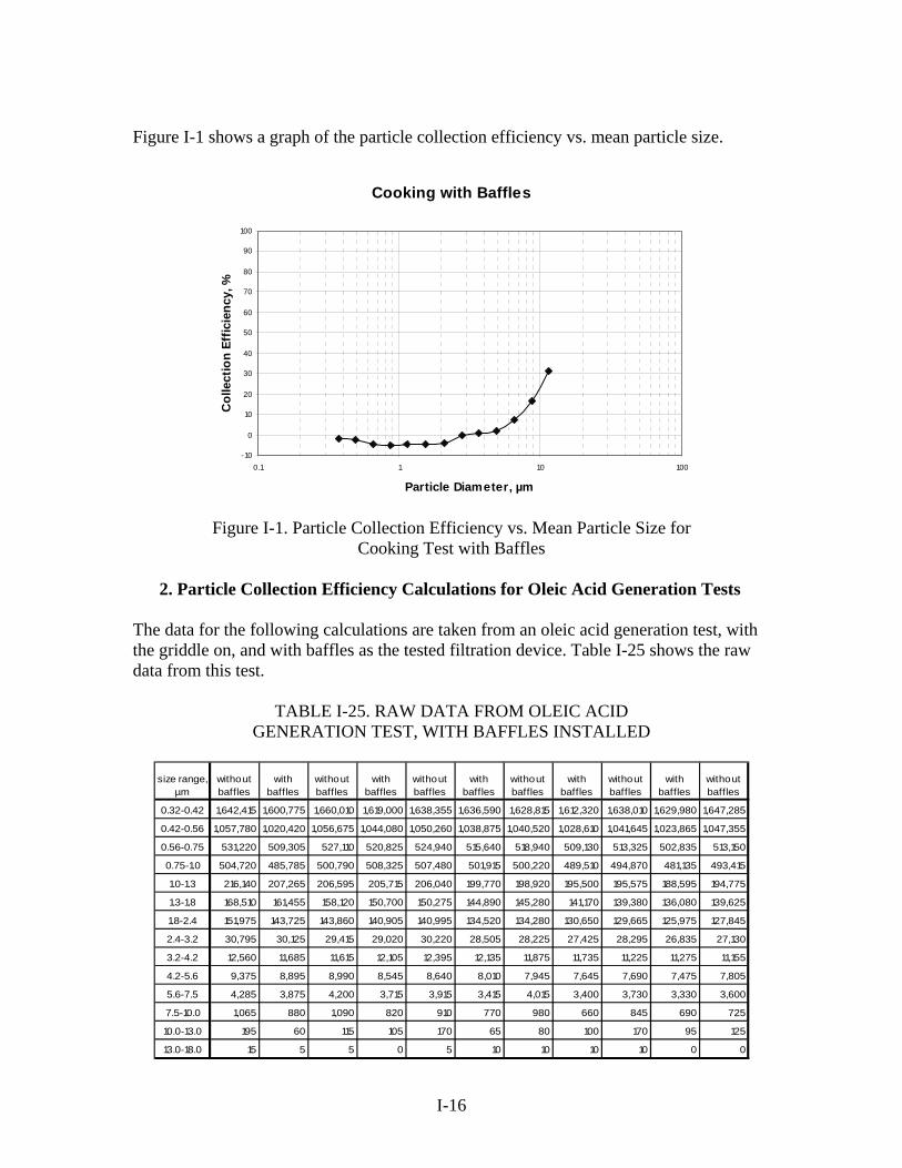
I-16

Figure I-1 shows a graph of the particle collection efficiency vs. mean particle size.

Cooking with Baffles

-10

0

10

20

30

40

50

60

70

80

90

100

0.1 1 10 100

Particle Diameter, µm

Col

lect

ion

Effic

ienc

y, %

Figure I-1. Particle Collection Efficiency vs. Mean Particle Size for

Cooking Test with Baffles

2. Particle Collection Efficiency Calculations for Oleic Acid Generation Tests The data for the following calculations are taken from an oleic acid generation test, with the griddle on, and with baffles as the tested filtration device. Table I-25 shows the raw data from this test.

TABLE I-25. RAW DATA FROM OLEIC ACID GENERATION TEST, WITH BAFFLES INSTALLED

0.32-0.42 1,642,415 1,600,775 1,660,010 1,619,000 1,638,355 1,636,590 1,628,815 1,612,320 1,638,010 1,629,980 1,647,285

0.42-0.56 1,057,780 1,020,420 1,056,675 1,044,080 1,050,260 1,038,875 1,040,520 1,028,610 1,041,645 1,023,865 1,047,355

0.56-0.75 531,220 509,305 527,110 520,825 524,940 515,640 518,940 509,130 513,325 502,835 513,150

0.75-1.0 504,720 485,785 500,790 508,325 507,480 501,915 500,220 489,510 494,870 481,135 493,415

1.0-1.3 216,140 207,265 206,595 205,715 206,040 199,770 198,920 195,500 195,575 188,595 194,775

1.3-1.8 168,510 161,455 158,120 150,700 150,275 144,890 145,280 141,170 139,380 136,080 139,625

1.8-2.4 151,975 143,725 143,860 140,905 140,995 134,520 134,280 130,650 129,665 125,975 127,845

2.4-3.2 30,795 30,125 29,415 29,020 30,220 28,505 28,225 27,425 28,295 26,835 27,130

3.2-4.2 12,560 11,685 11,615 12,105 12,395 12,135 11,875 11,735 11,225 11,275 11,155

4.2-5.6 9,375 8,895 8,990 8,545 8,640 8,010 7,945 7,645 7,690 7,475 7,805

5.6-7.5 4,285 3,875 4,200 3,715 3,915 3,415 4,015 3,400 3,730 3,330 3,600

7.5-10.0 1,065 880 1,090 820 910 770 980 660 845 690 725

10.0-13.0 195 60 115 105 170 65 80 100 170 95 125

13.0-18.0 15 5 5 0 5 10 10 10 10 0 0

without baffles

without baffles

without baffles

with baffles

with baffles

with baffles

with baffles

with baffles

size range, µm

without baffles

without baffles

without baffles

I-17

The background counts will not be taken into consideration for the oleic acid generation tests because of the difference in the test protocol from the cooking tests. This does not result in a significant change in results, as the particles are cleared from the room quickly between tests. All other calculations are identical. 1. Penetration calculations The estimated count without baffles that would have theoretically occurred at the same time as the count with baffles is determined from Equation G-25. Table I-26 shows the estimated count without baffles for each particle size range.

TABLE I-26. ESTIMATED PARTICLE COUNTS

0.32-0.42 1,651,213 1,649,183 1,633,585 1,633,413 1,642,6480.42-0.56 1,057,228 1,053,468 1,045,390 1,041,083 1,044,5000.56-0.75 529,165 526,025 521,940 516,133 513,2380.75-1.0 502,755 504,135 503,850 497,545 494,1431.0-1.3 211,368 206,318 202,480 197,248 195,1751.3-1.8 163,315 154,198 147,778 142,330 139,5031.8-2.4 147,918 142,428 137,638 131,973 128,7552.4-3.2 30,105 29,818 29,223 28,260 27,7133.2-4.2 12,088 12,005 12,135 11,550 11,1904.2-5.6 9,183 8,815 8,293 7,818 7,7485.6-7.5 4,243 4,058 3,965 3,873 3,6657.5-10.0 1,078 1,000 945 913 785

10.0-13.0 155 143 125 125 14813.0-18.0 10 5 8 10 5

size range, µm WO 1,e,t WO 2,e,t WO 3,e,t WO 4,e,t WO 5,e,t

The observed penetration is calculated using Equation G-27. Table I-27 shows the observed penetration for each particle size range.

I-18

TABLE I-27. OBSERVED PENETRATION FOR EACH TEST

0.32-0.42 0.969 0.982 1.002 0.987 0.9920.42-0.56 0.965 0.991 0.994 0.988 0.9800.56-0.75 0.962 0.990 0.988 0.986 0.9800.75-1.0 0.966 1.008 0.996 0.984 0.9741.0-1.3 0.981 0.997 0.987 0.991 0.9661.3-1.8 0.989 0.977 0.980 0.992 0.9751.8-2.4 0.972 0.989 0.977 0.990 0.9782.4-3.2 1.001 0.973 0.975 0.970 0.9683.2-4.2 0.967 1.008 1.000 1.016 1.0084.2-5.6 0.969 0.969 0.966 0.978 0.9655.6-7.5 0.913 0.916 0.861 0.878 0.9097.5-10.0 0.817 0.820 0.815 0.723 0.879

10.0-13.0 0.387 0.737 0.520 0.800 0.64413.0-18.0 0.500 0.000 1.333 1.000 0.000

P 4,o P 5,o

size range, µm P 1,o P 2,o P 3,o

The penetration is found using Equation G-28. The observed penetration for each test is simply averaged for each particle size range. Table I-28 shows the average observed penetration values for each particle size range.

TABLE I-28. AVERAGE OBSERVED PENETRATION

0.32-0.42 0.9860.42-0.56 0.9840.56-0.75 0.9810.75-1.0 0.9861.0-1.3 0.9841.3-1.8 0.9831.8-2.4 0.9812.4-3.2 0.9783.2-4.2 1.0004.2-5.6 0.9695.6-7.5 0.8957.5-10.0 0.811

10.0-13.0 0.61813.0-18.0 0.567

size range, µm oP

The standard deviation of the penetration is calculated using Equation G-29. Table I-29 shows the results of these calculations.

I-19

TABLE I-29. STANDARD DEVIATION OF PENETRATION

0.32-0.42 0.0120.42-0.56 0.0120.56-0.75 0.0110.75-1.0 0.0171.0-1.3 0.0121.3-1.8 0.0071.8-2.4 0.0082.4-3.2 0.0133.2-4.2 0.0194.2-5.6 0.0055.6-7.5 0.0247.5-10.0 0.056

10.0-13.0 0.16613.0-18.0 0.596

size range, µm δt

The 95% upper and lower confidence limits of the penetration are calculated using Equation G-31 and G-32. Table I-30 shows the values obtained for each particle size range.

TABLE I-30. 95% CONFIDENCE LIMITS OF THE PENETRATION

0.32-0.42 0.971 1.0010.42-0.56 0.969 0.9980.56-0.75 0.967 0.9950.75-1.0 0.965 1.0071.0-1.3 0.970 0.9991.3-1.8 0.974 0.9921.8-2.4 0.971 0.9912.4-3.2 0.961 0.9943.2-4.2 0.976 1.0244.2-5.6 0.963 0.9765.6-7.5 0.865 0.9267.5-10.0 0.742 0.880

10.0-13.0 0.411 0.82413.0-18.0 -0.174 1.307

size range, µm lclP uclP

The acceptance criteria for the error limit of the penetration is calculated from Equations G-35a, G-35b, and G-35c. Table I-31 shows the calculations and the corresponding criteria for each particle size range. Note that only the greater of the criteria values have been displayed.

I-20

TABLE I-31. ACCEPTANCE CRITERIA OF THE PENETRATION

0.32-0.42 0.01 0.070.42-0.56 0.01 0.070.56-0.75 0.01 0.070.75-1.0 0.02 0.071.0-1.3 0.01 0.071.3-1.8 0.01 0.071.8-2.4 0.01 0.072.4-3.2 0.02 0.073.2-4.2 0.02 0.154.2-5.6 0.01 0.155.6-7.5 0.03 0.187.5-10.0 0.07 0.16

10.0-13.0 0.2113.0-18.0 0.74

size range, µm stdev*t/sqrt(n) criteria

The minimum particle count criteria are determined using Equation G-37. Table I-32 shows the results of these calculations for each particle size range.

TABLE I-32. MINIMUM PARTICLE COUNT CRITERIA

0.32-0.42 8,210,0400.42-0.56 5,241,6680.56-0.75 2,606,5000.75-1.0 2,502,4281.0-1.3 1,012,5881.3-1.8 747,1231.8-2.4 688,7102.4-3.2 145,1183.2-4.2 58,9684.2-5.6 41,8555.6-7.5 19,8037.5-10.0 4,720

10.0-13.0 69513.0-18.0 38

size range, µm

particle count

As shown in Table I-32, the minimum particle counts have been satisfied in all size ranges except the 13.0-18.0 µm range. 2. Particle collection efficiency calculations The collection efficiency is calculated using Equation G-38. Table I-33 shows the collection efficiency for each particle size range.

I-21

TABLE I-33. COLLECTION EFFICIENCY OF BAFFLES

FOR OLEIC ACID GENERATION TEST

0.32-0.42 1.350.42-0.56 1.630.56-0.75 1.870.75-1.0 1.441.0-1.3 1.571.3-1.8 1.731.8-2.4 1.872.4-3.2 2.243.2-4.2 0.034.2-5.6 3.065.6-7.5 10.467.5-10.0 18.92

10.0-13.0 38.2413.0-18.0 43.33

size range, µm

collection efficiency, %

Figure I-2 shows a graph of the particle collection efficiency vs. mean particle size.

Oleic Acid with Baffles and Griddle On

0

10

20

30

40

50

60

70

80

90

100

0.1 1 10 100

Particle Diameter, µm

Col

lect

ion

Effic

ienc

y, %

Figure I-2. Particle Collection Efficiency vs. Mean Particle Size for

Oleic Acid Test with Baffles and Griddle On E. Particle Size Distribution Uncertainty from the Personal Cascade Impactor 1. The uncertainty associated with each impactor stage is determined using Equation H-1. Table I-34 shows the uncertainty associated with the mass measurements before mass

I-22

collection, after mass collection and desiccation, and the resulting uncertainty in the collected mass measurement. TABLE I-34. UNCERTAINTY IN THE MASS COLLECTED ON EACH PCI STAGE

Stage i ∆MBi (mg) ∆MAi (mg) ∆MCi (mg)

1 ±0.005 ±0.005 ±0.007 2 ±0.005 ±0.005 ±0.007 3 ±0.005 ±0.005 ±0.007 4 ±0.005 ±0.005 ±0.007 5 ±0.005 ±0.005 ±0.007 6 ±0.005 ±0.005 ±0.007 7 ±0.005 ±0.005 ±0.007 8 ±0.005 ±0.005 ±0.007 F ±0.005 ±0.005 ±0.007

The following is an example of the uncertainty calculation for stage 4.

( ) ( ) mg 007.0mg 005.0mg 005.0 224 ±=+=∆ CM

2. The uncertainties associated with the corrected collected particulate masses are determined using Equation H-2. The fourth stage from the cooking test with baffles is used for the sample calculation. The mass collected on the stage was 0.040 mg, the absolute uncertainty was ±0.007 mg, the correction factor was 0.07, or 7%, and the uncertainty in 1-CF was estimated to be ±0.020.

( )( )

mg 008.093.0

mg 040.0020.093.01mg 007.0

2

2

2

4 ±=⎥⎥⎦

⎤

⎢⎢⎣

⎡⎟⎟⎠

⎞⎜⎜⎝

⎛ −+⎥

⎦

⎤⎢⎣

⎡⎟⎠⎞

⎜⎝⎛=∆ CCM

Table I-35 shows the results for all the impactor stages, as well as the combined stage and filter.

I-23

TABLE I-35. UNCERTAINTIES ASSOCIATED WITH THE CORRECTED COLLECTED PARTICULATE MASS FOR EACH PCI STAGE

Stage i McCi (mg) ∆McCi (mg) 1-CF ∆(1-CF) ∆MCCi (mg)

1 0.008 ±0.007 0.760 ±0.020 ±0.009 2 0.003 ±0.007 0.870 ±0.020 ±0.008 3 0.038 ±0.007 0.920 ±0.020 ±0.008 4 0.040 ±0.007 0.930 ±0.020 ±0.008 5 0.055 ±0.007 0.950 ±0.020 ±0.007 6 0.059 ±0.007 0.965 ±0.020 ±0.007 7 0.011 ±0.007 0.970 ±0.020 ±0.007 8 0.065 ±0.007 0.995 ±0.010 ±0.007 F 0.217 ±0.007 1.000 ±0 ±0.007

4. The uncertainty associated with the total mass is determined using Equation H-3. Table I-35 shows the uncertainties associated with the corrected collected mass for each impactor stage. These values are used to solve Equation H-3.

( ) ( ) ( ) ( ) ( )( ) ( ) ( ) ( )

mg 023.0mg 007.0mg 007.0mg 007.0mg 007.0

mg 007.0mg 008.0mg 008.0mg 008.0mg 009.02222

22222

±=++++

++++=∆ TPM

F. Particle Size Distribution Uncertainty from the MOUDI 1. The uncertainty associated with each impactor stage is determined using Equation H-4. Table I-36 shows the uncertainty associated with the mass measurements before mass collection, after mass collection and desiccation, and the resulting uncertainty in the collected mass measurement.

TABLE I-36. UNCERTAINTY IN THE MASS COLLECTED ON EACH MOUDI STAGE

Stage i ∆MBi (mg) ∆MAi (mg) ∆MCi (mg)

1 ±0.005 ±0.005 ±0.007 2 ±0.005 ±0.005 ±0.007 3 ±0.005 ±0.005 ±0.007 4 ±0.005 ±0.005 ±0.007 5 ±0.005 ±0.005 ±0.007 6 ±0.005 ±0.005 ±0.007 7 ±0.005 ±0.005 ±0.007 8 ±0.005 ±0.005 ±0.007 9 ±0.005 ±0.005 ±0.007 10 ±0.005 ±0.005 ±0.007 11 ±0.005 ±0.005 ±0.007 F ±0.005 ±0.005 ±0.007

I-24

The following is an example of the uncertainty calculation for stage 4.

( ) ( ) mg 007.0mg 005.0mg 005.0 224 ±=+=∆ CM

2. The uncertainties associated with the corrected collected particulate masses are determined using Equation H-5. The fourth stage from the cooking test with baffles is used for the sample calculation. The mass collected on the stage was 3.199 mg, the absolute uncertainty was ±0.007 mg, the correction factor was 0.025, or 2.5 %, and the uncertainty in 1-CF was estimated to be ±0.020.

( )( )

mg 068.0975.0

mg 199.3020.0975.01mg 007.0

2

2

2

4 ±=⎥⎥⎦

⎤

⎢⎢⎣

⎡⎟⎟⎠

⎞⎜⎜⎝

⎛ −+⎥

⎦

⎤⎢⎣

⎡⎟⎠⎞

⎜⎝⎛=∆ CCM

Table I-37 shows the results for all the impactor stages, as well as the combined stage and filter.

TABLE I-37. UNCERTAINTIES ASSOCIATED WITH THE CORRECTED COLLECTED PARTICULATE MASS FOR EACH MOUDI STAGE

Stage i McCi (mg) ∆McCi (mg) 1-CF ∆(1-CF) ∆MCCi (mg)

1 0.053 ±0.007 0.670 ±0.020 ±0.011 2 0.144 ±0.007 0.800 ±0.020 ±0.010 3 1.183 ±0.007 0.910 ±0.020 ±0.030 4 3.199 ±0.007 0.975 ±0.020 ±0.068 5 1.961 ±0.007 0.990 ±0.010 ±0.021 6 1.034 ±0.007 0.990 ±0.010 ±0.013 7 0.274 ±0.007 0.990 ±0.010 ±0.008 8 0.162 ±0.007 0.990 ±0.010 ±0.007 9 0.364 ±0.007 0.990 ±0.010 ±0.008 10 0.079 ±0.007 0.970 ±0.020 ±0.007 11 0.078 ±0.007 0.920 ±0.020 ±0.008 F 0.035 ±0.007 1.000 ±0 ±0.007

3. The uncertainty associated with the total mass is determined using Equation H-6. Table I-37 shows the uncertainties associated with the corrected collected mass for each impactor stage. These values are used to solve Equation H-6.

( ) ( ) ( ) ( )( ) ( ) ( ) ( )( ) ( ) ( ) ( )

mg 082.0

mg 007.0mg 008.0mg 007.0mg 008.0

mg 007.0mg 008.0mg 013.0mg 021.0

mg 068.0mg 030.0mg 010.0mg 011.0

2222

2222

2222

±=

+++

++++

++++

=∆ TPM

I-25

G. Grease Vapor Uncertainty The uncertainty associated with the mass of collected grease vapor is determined using Equations H-7 though H-16. The first step to solving these equations is determining the absolute uncertainty associated with the mass of each container, before and after collection and evaporation. The larger of the uncertainties determined using Equations H-15 and H-16 is used for the remaining calculations. The uncertainty found using Equation H-15 is identical for all container weights. The absolute uncertainty in the scale was found to be ±0.5 mg, and there were 3 measurements for each container.

mg 3.03mg 5.0

__ ±==∆M

Equation H-16 gives the standard deviation associated with the average weight of each container, for weightings before and after collection and evaporation. Table I-38 shows the measured, average, and standard deviation of the weights associated with each container.

TABLE I-38. STANDARD DEVIATION ASSOCIATED WITH THE WEIGHT OF EACH CONTAINER USED FOR GREASE VAPOR MASS DETERMINATION

Before 1 2 3 4 5 6 7 81 (g) 69.0152 63.8973 67.1594 62.3552 67.0133 69.7857 68.2992 68.48192 (g) 69.0151 63.8971 67.1594 62.3550 67.0137 69.7862 68.2991 68.48183 (g) 69.0151 63.8975 67.1593 62.3551 67.0135 69.7865 68.2992 68.4818

Ave. (g) 69.0151 63.8973 67.1594 62.3551 67.0135 69.7861 68.2992 68.4818STD (mg) 0.06 0.20 0.06 0.10 0.20 0.40 0.06 0.06

After 1 2 3 4 5 6 7 81 (g) 69.0177 63.8989 67.1608 62.3588 67.0168 69.7898 68.3028 68.48422 (g) 69.0176 63.8992 67.1608 62.3588 67.0168 69.7899 68.3033 68.48453 (g) 69.0174 63.8992 67.1609 62.3587 67.0167 69.7897 68.3031 68.4842

Ave. (g) 69.0176 63.8991 67.1608 62.3588 67.0168 69.7898 68.3031 68.4843STD (mg) 0.15 0.17 0.06 0.06 0.06 0.10 0.25 0.17

Container

Comparing the standard deviations shown in Table I-38 to the uncertainty found using Equation H-15 shows that the value found using Equation H-15 is always larger than the standard deviations. Equation H-14 is used to determine the uncertainty associated with the net mass collected in a given container. Because the uncertainty found using Equation H-15 is the applicable uncertainty for the average mass of each container, the result of Equation H-14 is also applicable to the uncertainty in the net mass collected in each container.

( ) ( ) mg 4.0mg 3.0mg 3.0 22 ±=+=∆ icontvM

I-26

Equations H-8 through H-13, which give the absolute uncertainty associated with each collection area, are all dependent on the uncertainty associated with the net mass from two particular containers. Because these containers all have the same uncertainty, the uncertainties associated with each collection area are identical.

( ) ( ) mg 6.0mg 4.0mg 4.0 22 ±=+=∆ areacollectionvM

The uncertainty associated with the total mass of grease vapor collected is determined using Equation H-7.

( ) ( ) ( )( ) ( ) ( )

mg 5.1mg 6.0mg 6.0mg 6.0

mg 6.0mg 6.0mg 6.0222

222

=++

+++=∆ totalvM

J-1

APPENDIX J

FOOD PRODUCT TYPE AND DESCRIPTION

J-2

FOOD PRODUCT TYPE AND DESCRIPTION

TABLE J-1. DESCRIPTION OF FOOD PRODUCT

FOOD PRODUCT DESCRIPTION Beef hamburgers

(Whopper hamburger patties

supplied by Burger King)

Pure beef, finished grind, frozen Weight: 0.25 lb. (0.11 kg) Thickness: 0.25 in. (0.64 cm) Diameter: 6 in. ± 0.25 in. (15.2 cm ± 0.64 cm) Fat content: 23 ± 2 % Moisture content: 60 ± 2 % Adheres to ASTM 1275-99

Documents

APPENDIX A SAMPLING AND INSTRUMENTATION EQUIPMENT … · SAMPLING AND INSTRUMENTATION EQUIPMENT 1. ... 4. 36 x 28 x 1 in. ... to log-Tchebycheff rule TABLE B-1