A-1

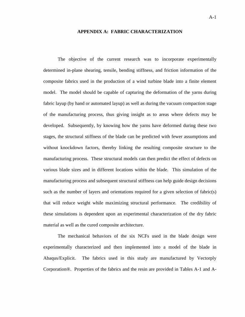
APPENDIX A: FABRIC CHARACTERIZATION

The objective of the current research was to incorporate experimentally

determined in-plane shearing, tensile, bending stiffness, and friction information of the

composite fabrics used in the production of a wind turbine blade into a finite element

model. The model should be capable of capturing the deformation of the yarns during

fabric layup (by hand or automated layup) as well as during the vacuum compaction stage

of the manufacturing process, thus giving insight as to areas where defects may be

developed. Subsequently, by knowing how the yarns have deformed during these two

stages, the structural stiffness of the blade can be predicted with fewer assumptions and

without knockdown factors, thereby linking the resulting composite structure to the

manufacturing process. These structural models can then predict the effect of defects on

various blade sizes and in different locations within the blade. This simulation of the

manufacturing process and subsequent structural stiffness can help guide design decisions

such as the number of layers and orientations required for a given selection of fabric(s)

that will reduce weight while maximizing structural performance. The credibility of

these simulations is dependent upon an experimental characterization of the dry fabric

material as well as the cured composite architecture.

The mechanical behaviors of the six NCFs used in the blade design were

experimentally characterized and then implemented into a model of the blade in

Abaqus/Explicit. The fabrics used in this study are manufactured by Vectorply

Corporation®. Properties of the fabrics and the resin are provided in Tables A-1 and A-

A-2

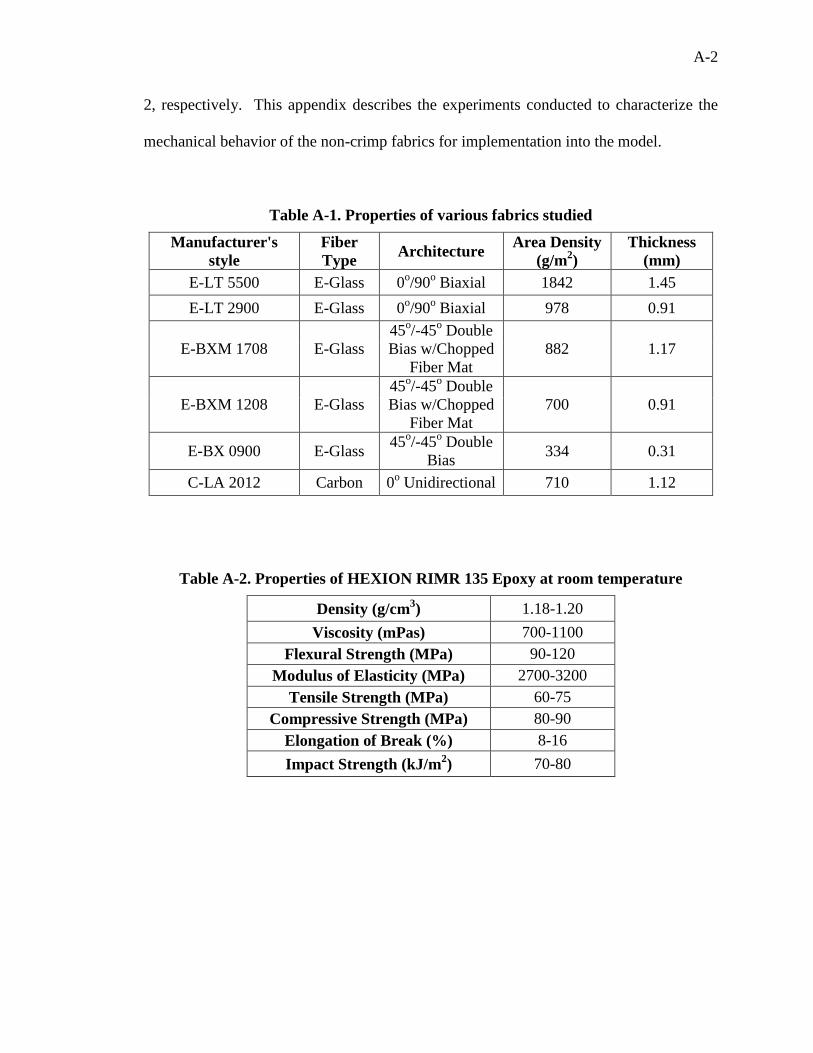
2, respectively. This appendix describes the experiments conducted to characterize the

mechanical behavior of the non-crimp fabrics for implementation into the model.

Table A-1. Properties of various fabrics studied

Manufacturer's

style

Fiber

Type Architecture

Area Density

(g/m2)

Thickness

(mm)

E-LT 5500 E-Glass 0o/90

o Biaxial 1842 1.45

E-LT 2900 E-Glass 0o/90

o Biaxial 978 0.91

E-BXM 1708 E-Glass

45o/-45

o Double

Bias w/Chopped

Fiber Mat

882 1.17

E-BXM 1208 E-Glass

45o/-45

o Double

Bias w/Chopped

Fiber Mat

700 0.91

E-BX 0900 E-Glass 45

o/-45

o Double

Bias 334 0.31

C-LA 2012 Carbon 0o Unidirectional 710 1.12

Table A-2. Properties of HEXION RIMR 135 Epoxy at room temperature

Density (g/cm3) 1.18-1.20

Viscosity (mPas) 700-1100

Flexural Strength (MPa) 90-120

Modulus of Elasticity (MPa) 2700-3200

Tensile Strength (MPa) 60-75

Compressive Strength (MPa) 80-90

Elongation of Break (%) 8-16

Impact Strength (kJ/m2) 70-80

A-3

1 DRY FABRIC MODELING

The discrete approach in the current research utilized a commercially available

finite element package (Abaqus), where standard beam and shell elements were used in

conjunction with a user-defined material subroutine to model the fabric blanks using a

hypoelastic description. The use of these common element types allows a similar

approach to be extended to other popular finite element packages with user material

subroutine capabilities such as LS-DYNA and ANSYS, without the need for any special-

purpose element types. Such an approach is attractive to industry because the method

uses commercially available finite element codes.

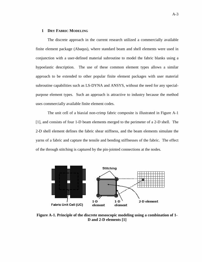
The unit cell of a biaxial non-crimp fabric composite is illustrated in Figure A-1

[1], and consists of four 1-D beam elements merged to the perimeter of a 2-D shell. The

2-D shell element defines the fabric shear stiffness, and the beam elements simulate the

yarns of a fabric and capture the tensile and bending stiffnesses of the fabric. The effect

of the through stitching is captured by the pin-jointed connections at the nodes.

Figure A-1. Principle of the discrete mesoscopic modeling using a combination of 1-

D and 2-D elements [1]

A-4

Regressions of experimental data were used to conclude empirical models that

were then implemented as user-defined material subroutines to capture the mechanical

behavior of the fabric material in the finite element solver [2]. Finite element models of

the various tests were completed to validate that the fabric model behavior can be

properly simulated using the finite element method. Additionally, the finite element

method allows for contact to be defined between layers of fabric [3].

2 FABRIC ARCHITECTURE

Table A-1 summarized the six non-crimp fabrics used in the manufacture of the 9-

meter CX-100 wind turbine blade.

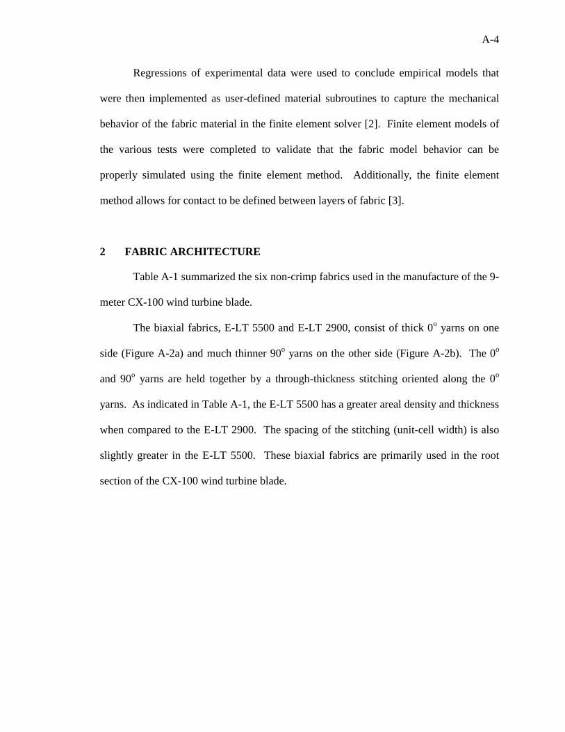
The biaxial fabrics, E-LT 5500 and E-LT 2900, consist of thick 0o yarns on one

side (Figure A-2a) and much thinner 90o yarns on the other side (Figure A-2b). The 0

o

and 90o yarns are held together by a through-thickness stitching oriented along the 0

o

yarns. As indicated in Table A-1, the E-LT 5500 has a greater areal density and thickness

when compared to the E-LT 2900. The spacing of the stitching (unit-cell width) is also

slightly greater in the E-LT 5500. These biaxial fabrics are primarily used in the root

section of the CX-100 wind turbine blade.

A-5

Figure A-2. Biaxial NCF architecture

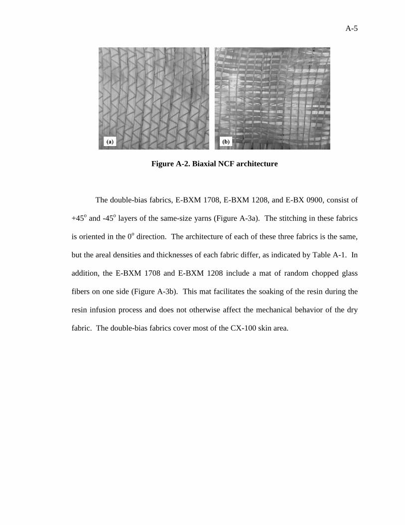
The double-bias fabrics, E-BXM 1708, E-BXM 1208, and E-BX 0900, consist of

+45o and -45

o layers of the same-size yarns (Figure A-3a). The stitching in these fabrics

is oriented in the 0o direction. The architecture of each of these three fabrics is the same,

but the areal densities and thicknesses of each fabric differ, as indicated by Table A-1. In

addition, the E-BXM 1708 and E-BXM 1208 include a mat of random chopped glass

fibers on one side (Figure A-3b). This mat facilitates the soaking of the resin during the

resin infusion process and does not otherwise affect the mechanical behavior of the dry

fabric. The double-bias fabrics cover most of the CX-100 skin area.

A-6

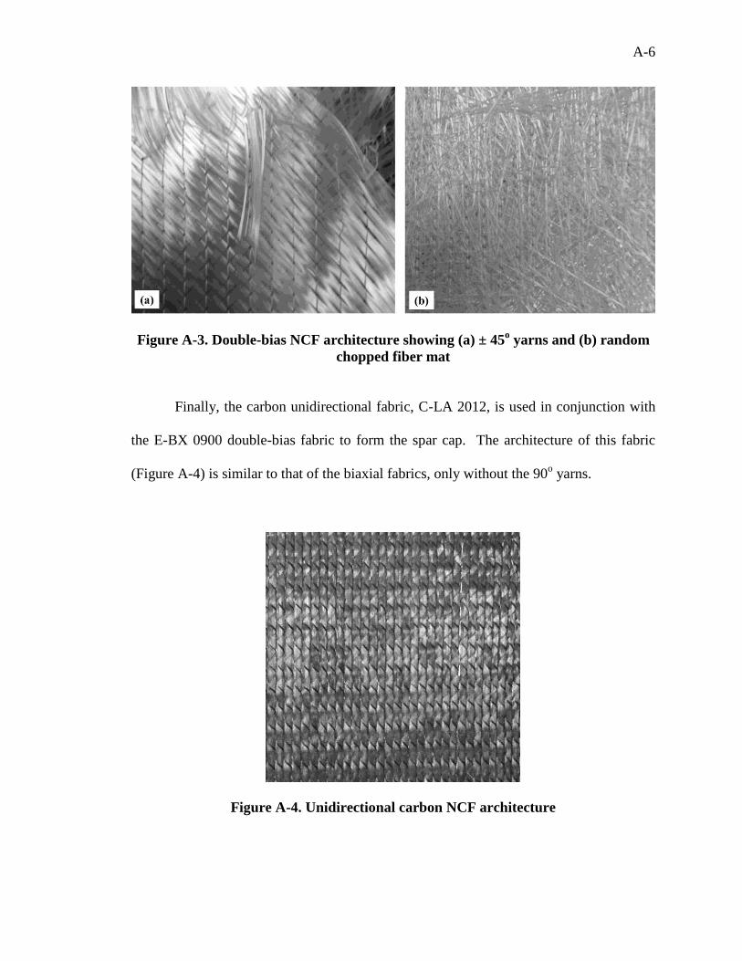
Figure A-3. Double-bias NCF architecture showing (a) ± 45o yarns and (b) random

chopped fiber mat

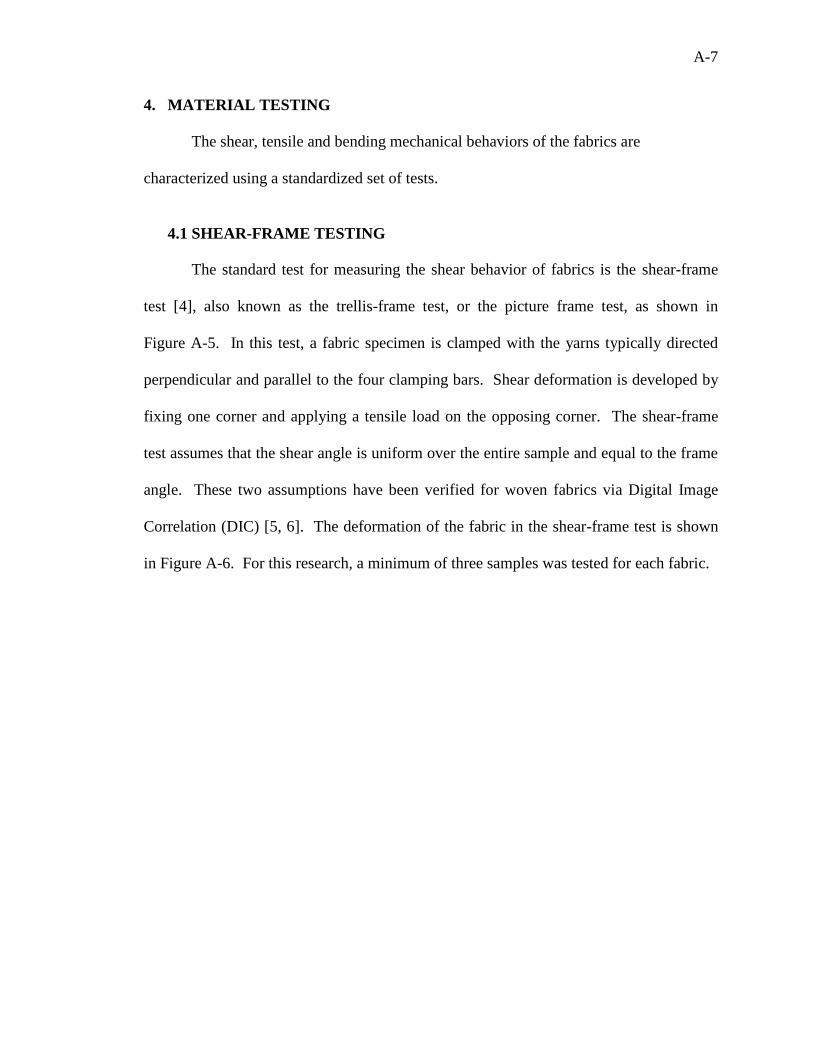
Finally, the carbon unidirectional fabric, C-LA 2012, is used in conjunction with

the E-BX 0900 double-bias fabric to form the spar cap. The architecture of this fabric

(Figure A-4) is similar to that of the biaxial fabrics, only without the 90o yarns.

Figure A-4. Unidirectional carbon NCF architecture

A-7

4. MATERIAL TESTING

The shear, tensile and bending mechanical behaviors of the fabrics are

characterized using a standardized set of tests.

4.1 SHEAR-FRAME TESTING

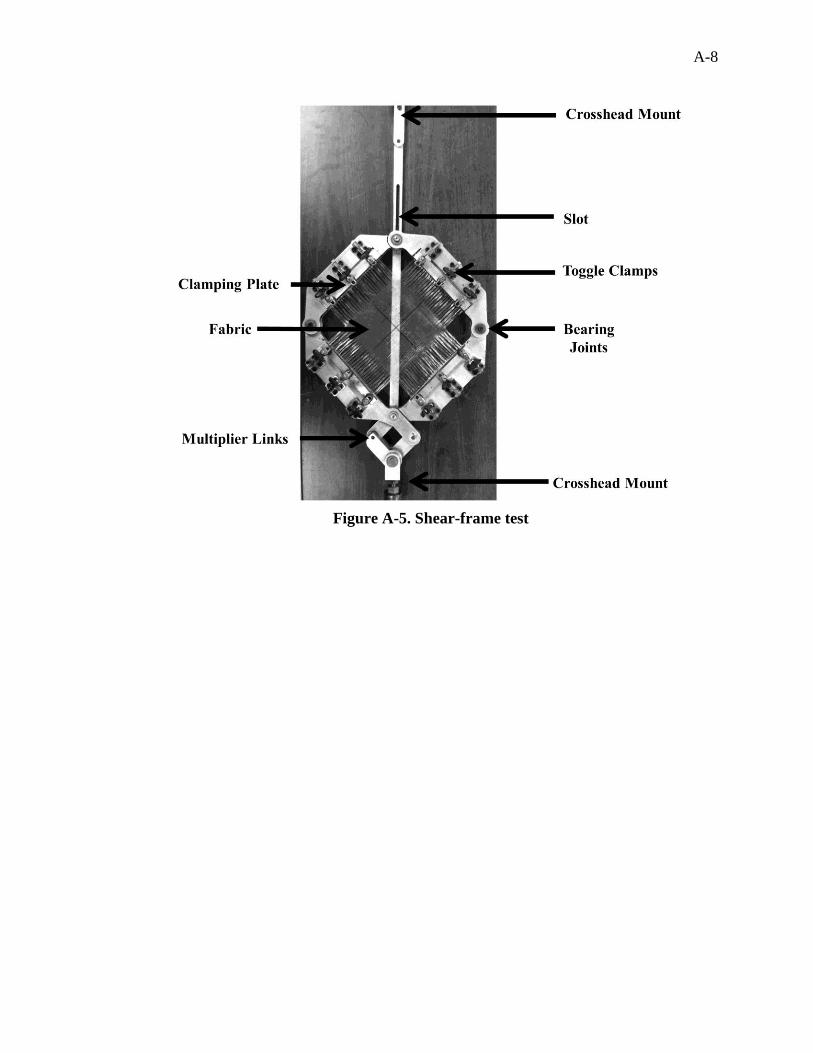
The standard test for measuring the shear behavior of fabrics is the shear-frame

test [4], also known as the trellis-frame test, or the picture frame test, as shown in

Figure A-5. In this test, a fabric specimen is clamped with the yarns typically directed

perpendicular and parallel to the four clamping bars. Shear deformation is developed by

fixing one corner and applying a tensile load on the opposing corner. The shear-frame

test assumes that the shear angle is uniform over the entire sample and equal to the frame

angle. These two assumptions have been verified for woven fabrics via Digital Image

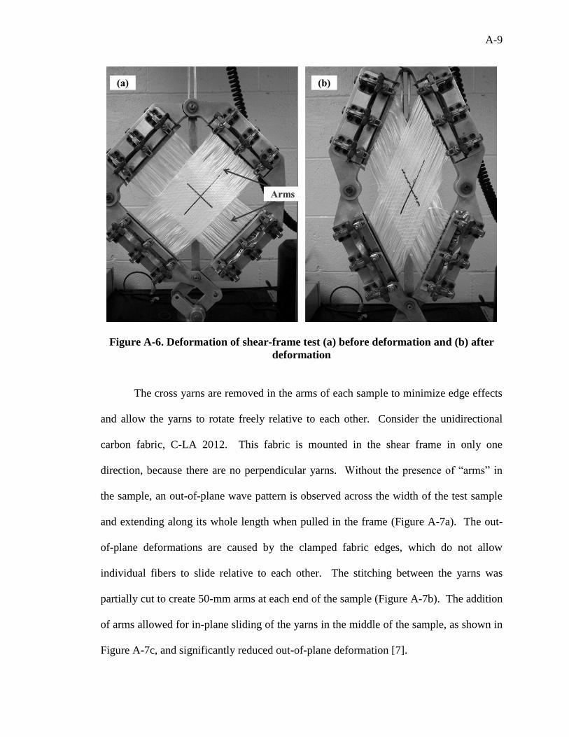
Correlation (DIC) [5, 6]. The deformation of the fabric in the shear-frame test is shown

in Figure A-6. For this research, a minimum of three samples was tested for each fabric.

A-8

Figure A-5. Shear-frame test

A-9

Figure A-6. Deformation of shear-frame test (a) before deformation and (b) after

deformation

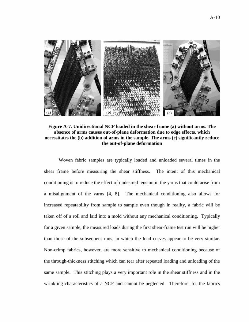
The cross yarns are removed in the arms of each sample to minimize edge effects

and allow the yarns to rotate freely relative to each other. Consider the unidirectional

carbon fabric, C-LA 2012. This fabric is mounted in the shear frame in only one

direction, because there are no perpendicular yarns. Without the presence of “arms” in

the sample, an out-of-plane wave pattern is observed across the width of the test sample

and extending along its whole length when pulled in the frame (Figure A-7a). The out-

of-plane deformations are caused by the clamped fabric edges, which do not allow

individual fibers to slide relative to each other. The stitching between the yarns was

partially cut to create 50-mm arms at each end of the sample (Figure A-7b). The addition

of arms allowed for in-plane sliding of the yarns in the middle of the sample, as shown in

Figure A-7c, and significantly reduced out-of-plane deformation [7].

A-10

Figure A-7. Unidirectional NCF loaded in the shear frame (a) without arms. The

absence of arms causes out-of-plane deformation due to edge effects, which

necessitates the (b) addition of arms in the sample. The arms (c) significantly reduce

the out-of-plane deformation

Woven fabric samples are typically loaded and unloaded several times in the

shear frame before measuring the shear stiffness. The intent of this mechanical

conditioning is to reduce the effect of undesired tension in the yarns that could arise from

a misalignment of the yarns [4, 8]. The mechanical conditioning also allows for

increased repeatability from sample to sample even though in reality, a fabric will be

taken off of a roll and laid into a mold without any mechanical conditioning. Typically

for a given sample, the measured loads during the first shear-frame test run will be higher

than those of the subsequent runs, in which the load curves appear to be very similar.

Non-crimp fabrics, however, are more sensitive to mechanical conditioning because of

the through-thickness stitching which can tear after repeated loading and unloading of the

same sample. This stitching plays a very important role in the shear stiffness and in the

wrinkling characteristics of a NCF and cannot be neglected. Therefore, for the fabrics

A-11

studied in this research, the samples were not mechanically conditioned, and the first

load-displacement curve was taken as the representative shear deformation curve.

The measured load is converted to a force that is normalized by the length of the

frame. This normalization accounts for various shear-frame sizes and allows for

comparison between labs with differing frame sizes. The normalized force can then be

divided by the thickness of the fabric sample to obtain the shear stress. Similarly, the

shear angle can be determined by knowing the length of the frame, length of the fabric

sample, and the measured displacement data. This angle can then be converted to a

logarithmic shear strain, which is consistent with the shear strain definition used by the

finite element code. After testing a minimum of three samples, the average shear stress

and logarithmic strain are calculated and plotted with error bars of one standard

deviation.

After all of the stress-logarithmic strain plots have been generated, polynomial fits

are made to these curves. These functions are implemented into Abaqus/Explicit via its

user-defined material subroutine, VUMAT, to capture the shear behavior of each fabric.

Abaqus/Explicit uses rate-independent constitutive equations, also called hypoelastic

laws, to model large deformation and strains. Stresses are updated using:

11 t

ij

t

ij

t

ij (1)

21

1 .

t

klijkl

t

ij C (2)

where ijt+1

is the stress increment at time step t+1, Cijkl is the constitutive matrix and

klt+½

is the midpoint strain increment obtained from the integration of the strain rate

tensor. The custom constitutive models obtained through regressions of experimental

A-12

data and implemented into the VUMAT subroutine are linked with the overall solver to

update the stress (Equation 2). The strain increment, klt+½

, is given by the solver to

VUMAT that subsequently returns the corresponding stress increment to the solver. The

stress update is made in the local reference frame for the element, i.e. a co-rotational

frame that rotates with the element. The summation of the strain increments gives a

logarithmic (or true) strain in the principal-stretch directions. Details associated with the

constitutive equations as they pertain to the 1-D and 2-D elements of the current unit-cell

model are provided in [2]. The VUMAT subroutine is provided in Appendix A.

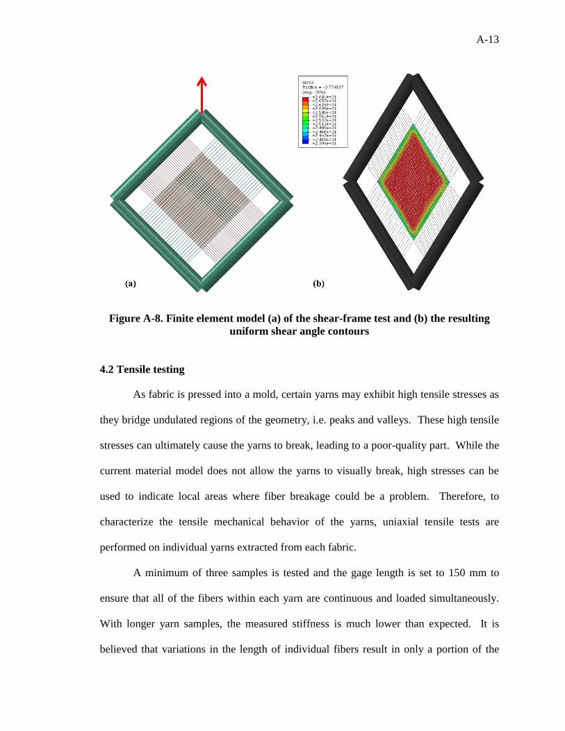
A finite element model of the fabric shear-frame test, including the “arms” of the

specimens, is generated to ensure that the 2-D shell elements are accurately capturing the

shear stiffness of each fabric (Figure A-8a). The arms are modeled using 1-D beam

elements, and the frame is modeled using four aluminum trusses with a cross section of

500 mm2. The constants that define the tangent shear modulus are obtained by deriving

the polynomial fits of the experimental stress-logarithmic strain curves and are defined in

the Abaqus input file material card. The model correlates with the assumption of pure

shear in the fabric sample (Figure A-8b).

A-13

Figure A-8. Finite element model (a) of the shear-frame test and (b) the resulting

uniform shear angle contours

4.2 Tensile testing

As fabric is pressed into a mold, certain yarns may exhibit high tensile stresses as

they bridge undulated regions of the geometry, i.e. peaks and valleys. These high tensile

stresses can ultimately cause the yarns to break, leading to a poor-quality part. While the

current material model does not allow the yarns to visually break, high stresses can be

used to indicate local areas where fiber breakage could be a problem. Therefore, to

characterize the tensile mechanical behavior of the yarns, uniaxial tensile tests are

performed on individual yarns extracted from each fabric.

A minimum of three samples is tested and the gage length is set to 150 mm to

ensure that all of the fibers within each yarn are continuous and loaded simultaneously.

With longer yarn samples, the measured stiffness is much lower than expected. It is

believed that variations in the length of individual fibers result in only a portion of the

A-14

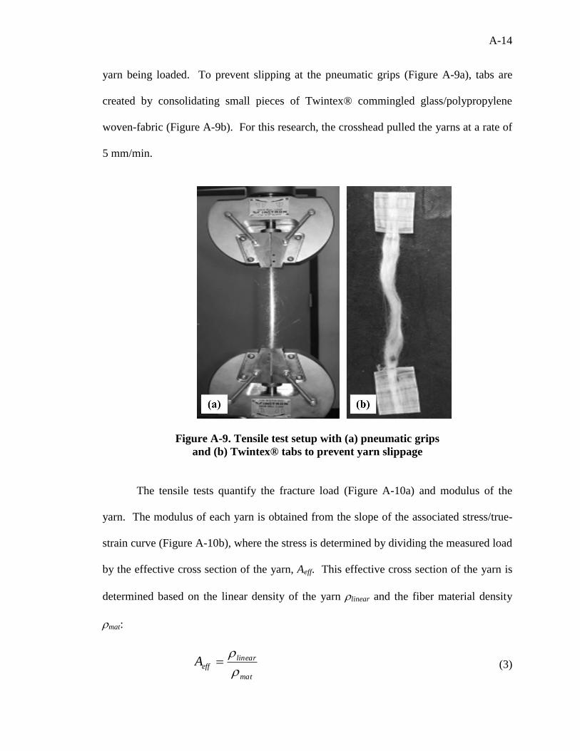
yarn being loaded. To prevent slipping at the pneumatic grips (Figure A-9a), tabs are

created by consolidating small pieces of Twintex® commingled glass/polypropylene

woven-fabric (Figure A-9b). For this research, the crosshead pulled the yarns at a rate of

5 mm/min.

Figure A-9. Tensile test setup with (a) pneumatic grips

and (b) Twintex® tabs to prevent yarn slippage

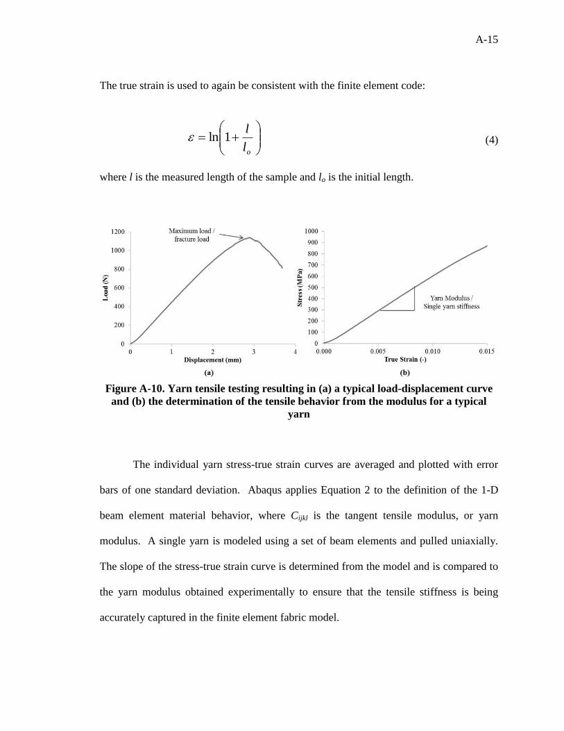
The tensile tests quantify the fracture load (Figure A-10a) and modulus of the

yarn. The modulus of each yarn is obtained from the slope of the associated stress/true-

strain curve (Figure A-10b), where the stress is determined by dividing the measured load

by the effective cross section of the yarn, Aeff. This effective cross section of the yarn is

determined based on the linear density of the yarn linear and the fiber material density

mat:

mat

lineareffA

(3)

A-15

The true strain is used to again be consistent with the finite element code:

ol

l1ln (4)

where l is the measured length of the sample and lo is the initial length.

Figure A-10. Yarn tensile testing resulting in (a) a typical load-displacement curve

and (b) the determination of the tensile behavior from the modulus for a typical

yarn

The individual yarn stress-true strain curves are averaged and plotted with error

bars of one standard deviation. Abaqus applies Equation 2 to the definition of the 1-D

beam element material behavior, where Cijkl is the tangent tensile modulus, or yarn

modulus. A single yarn is modeled using a set of beam elements and pulled uniaxially.

The slope of the stress-true strain curve is determined from the model and is compared to

the yarn modulus obtained experimentally to ensure that the tensile stiffness is being

accurately captured in the finite element fabric model.

A-16

4.3 Bending stiffness test

To use the finite element method for predicting the formation of in-plane and/or

out-of-plane waviness during the manufacture of composite wind turbine blades, the

overall mechanical behavior of the composite fabric reinforcements must be thoroughly

defined. The in-plane shearing behavior is often used as an indicator via the “locking

angle” as to when wrinkles may develop in the form of in-plane and/or out-of-plane

waves. As yarns rotate relative to one another, they eventually reach a point where they

can no longer rotate in-plane and must buckle out-of-plane. However, it has been shown

that simply relating wrinkling to the shear angle is not sufficient. The formation of

wrinkles and/or waves depends on the combination of in-plane shear, tension and

bending behaviors of the fabric [9]. Thus, it is important to characterize the bending

stiffness of the dry non-crimp fabrics.

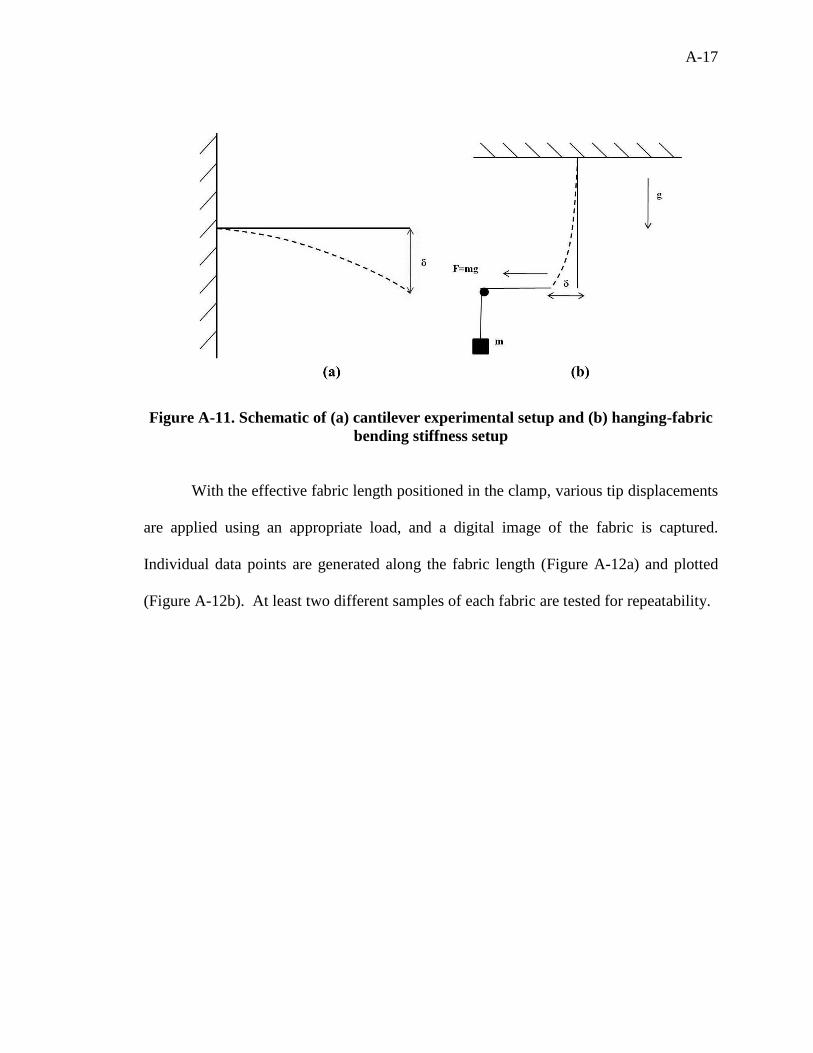
When characterizing the dry fabric bending stiffness, a cantilever “beam” method

is often used [10], where the fabric is allowed to bend due to its own weight (Figure A-

11a). However, depending on the length of the sample, the effective direction of the

distributed load on the sample changes due to the large deformations, and thus, a single

value for the fabric bending stiffness cannot be concluded for all lengths despite efforts to

compensate for the effect of gravity. An alternate method for characterizing the bending

stiffness is to align the length of the beam with gravity and thereby reduce the nonlinear

loading effects [11]. Fabric samples are clamped at one end and hung vertically. A

horizontal load is applied to displace the tip of the fabric a known amount. This load is

applied by attaching masses to a string tied to the tip of the fabric sample (Figure A-11b).

A-17

Figure A-11. Schematic of (a) cantilever experimental setup and (b) hanging-fabric

bending stiffness setup

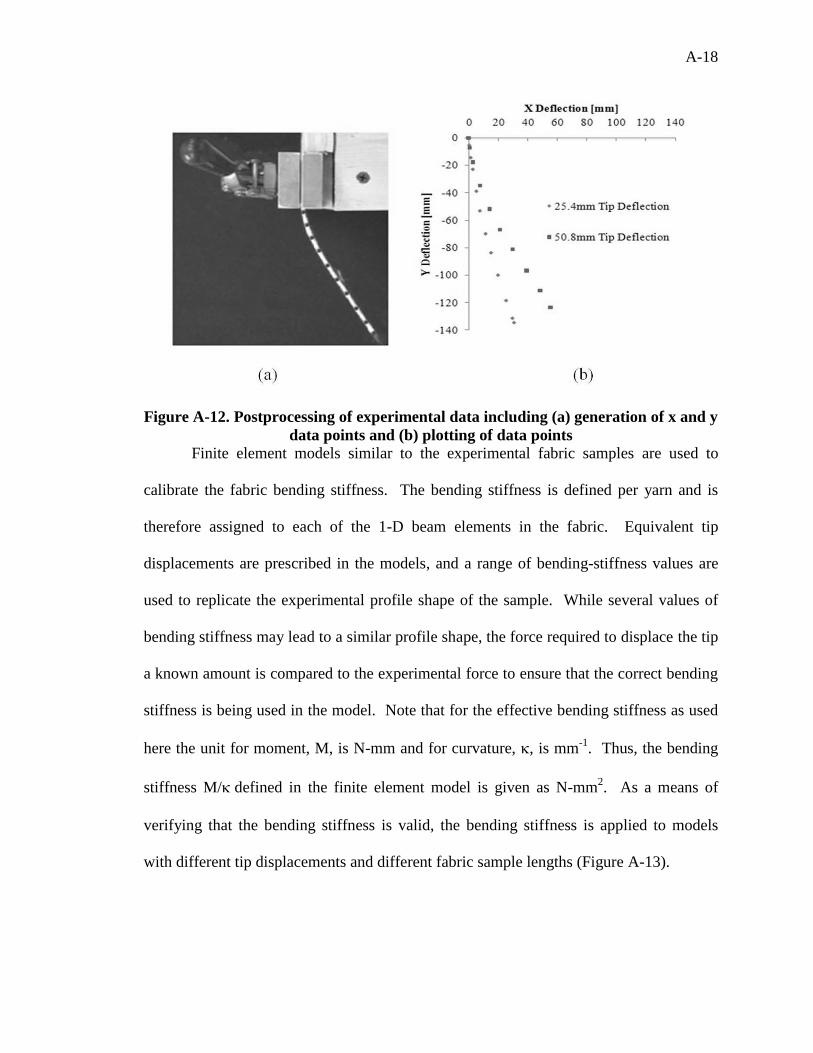
With the effective fabric length positioned in the clamp, various tip displacements

are applied using an appropriate load, and a digital image of the fabric is captured.

Individual data points are generated along the fabric length (Figure A-12a) and plotted

(Figure A-12b). At least two different samples of each fabric are tested for repeatability.

A-18

Figure A-12. Postprocessing of experimental data including (a) generation of x and y

data points and (b) plotting of data points

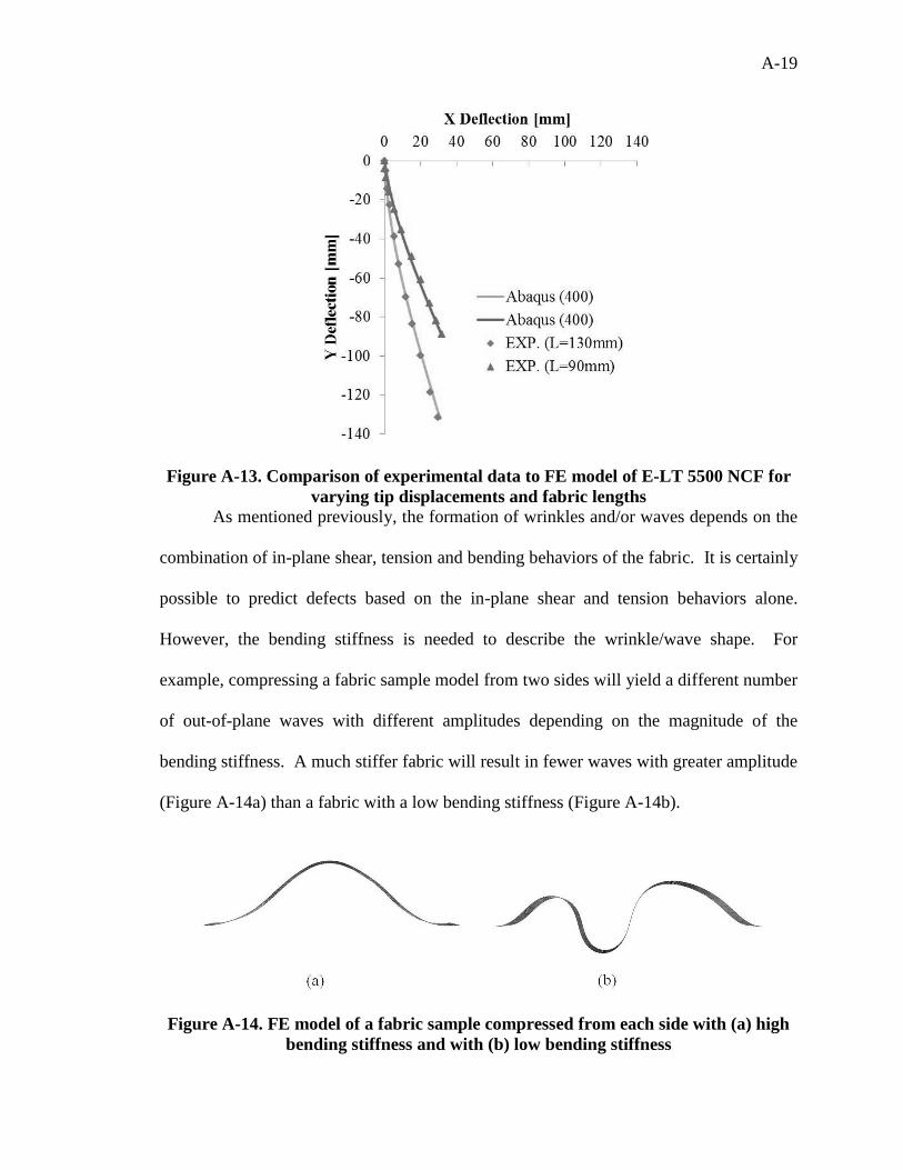
Finite element models similar to the experimental fabric samples are used to

calibrate the fabric bending stiffness. The bending stiffness is defined per yarn and is

therefore assigned to each of the 1-D beam elements in the fabric. Equivalent tip

displacements are prescribed in the models, and a range of bending-stiffness values are

used to replicate the experimental profile shape of the sample. While several values of

bending stiffness may lead to a similar profile shape, the force required to displace the tip

a known amount is compared to the experimental force to ensure that the correct bending

stiffness is being used in the model. Note that for the effective bending stiffness as used

here the unit for moment, M, is N-mm and for curvature, , is mm-1

. Thus, the bending

stiffness M/defined in the finite element model is given as N-mm2. As a means of

verifying that the bending stiffness is valid, the bending stiffness is applied to models

with different tip displacements and different fabric sample lengths (Figure A-13).

A-19

Figure A-13. Comparison of experimental data to FE model of E-LT 5500 NCF for

varying tip displacements and fabric lengths

As mentioned previously, the formation of wrinkles and/or waves depends on the

combination of in-plane shear, tension and bending behaviors of the fabric. It is certainly

possible to predict defects based on the in-plane shear and tension behaviors alone.

However, the bending stiffness is needed to describe the wrinkle/wave shape. For

example, compressing a fabric sample model from two sides will yield a different number

of out-of-plane waves with different amplitudes depending on the magnitude of the

bending stiffness. A much stiffer fabric will result in fewer waves with greater amplitude

(Figure A-14a) than a fabric with a low bending stiffness (Figure A-14b).

Figure A-14. FE model of a fabric sample compressed from each side with (a) high

bending stiffness and with (b) low bending stiffness

A-20

In the current unit-cell modeling approach, the 1-D beam elements carry the

bending stiffness of the fabric yarns. Without explicitly defining the bending stiffness as

part of the beam section properties, Abaqus will by default consider the product of the

elastic modulus, E, and the area moment of inertia, I, of the elements to define the

bending stiffness. This default definition is typically much higher than the measured

bending stiffness.

A-21

5 MATERIAL TEST RESULTS

The results of the material characterization results are summarized in the

following sections.

5.1 SHEAR FRAME TEST

The in-plane shearing of the fabric yarns is the principal mode of deformation as a

fabric layer conforms to the shape of a double-curvature geometry. This in-plane

shearing results in a change of the angle between the initially orthogonal yarns of a

biaxial non-crimp fabric. The shear-frame test is used to characterize this in-plane

shearing behavior. The measured load-displacement data are converted to stress-

logarithmic shear strain to be consistent with the definition of shear strain as used by the

finite element code. After testing a minimum of three samples, the average shear stress

and logarithmic strain are calculated and plotted with error bars of one standard deviation

(Figure A-15).

A-22

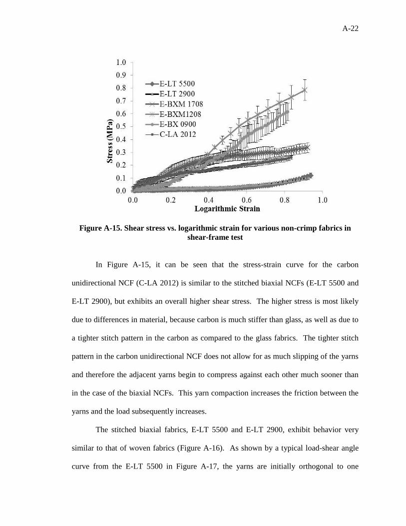
Figure A-15. Shear stress vs. logarithmic strain for various non-crimp fabrics in

shear-frame test

In Figure A-15, it can be seen that the stress-strain curve for the carbon

unidirectional NCF (C-LA 2012) is similar to the stitched biaxial NCFs (E-LT 5500 and

E-LT 2900), but exhibits an overall higher shear stress. The higher stress is most likely

due to differences in material, because carbon is much stiffer than glass, as well as due to

a tighter stitch pattern in the carbon as compared to the glass fabrics. The tighter stitch

pattern in the carbon unidirectional NCF does not allow for as much slipping of the yarns

and therefore the adjacent yarns begin to compress against each other much sooner than

in the case of the biaxial NCFs. This yarn compaction increases the friction between the

yarns and the load subsequently increases.

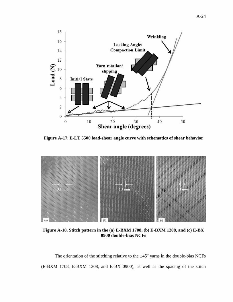
The stitched biaxial fabrics, E-LT 5500 and E-LT 2900, exhibit behavior very

similar to that of woven fabrics (Figure A-16). As shown by a typical load-shear angle

curve from the E-LT 5500 in Figure A-17, the yarns are initially orthogonal to one

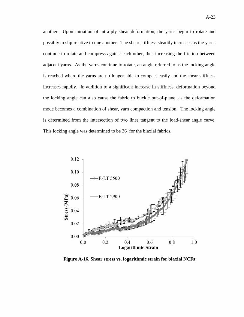
A-23

another. Upon initiation of intra-ply shear deformation, the yarns begin to rotate and

possibly to slip relative to one another. The shear stiffness steadily increases as the yarns

continue to rotate and compress against each other, thus increasing the friction between

adjacent yarns. As the yarns continue to rotate, an angle referred to as the locking angle

is reached where the yarns are no longer able to compact easily and the shear stiffness

increases rapidly. In addition to a significant increase in stiffness, deformation beyond

the locking angle can also cause the fabric to buckle out-of-plane, as the deformation

mode becomes a combination of shear, yarn compaction and tension. The locking angle

is determined from the intersection of two lines tangent to the load-shear angle curve.

This locking angle was determined to be 36o for the biaxial fabrics.

Figure A-16. Shear stress vs. logarithmic strain for biaxial NCFs

A-24

Figure A-17. E-LT 5500 load-shear angle curve with schematics of shear behavior

Figure A-18. Stitch pattern in the (a) E-BXM 1708, (b) E-BXM 1208, and (c) E-BX

0900 double-bias NCFs

The orientation of the stitching relative to the ±45o yarns in the double-bias NCFs

(E-BXM 1708, E-BXM 1208, and E-BX 0900), as well as the spacing of the stitch

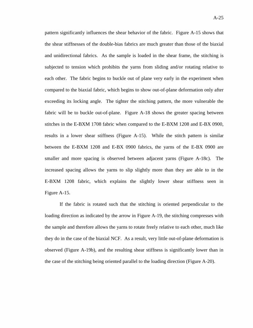
A-25

pattern significantly influences the shear behavior of the fabric. Figure A-15 shows that

the shear stiffnesses of the double-bias fabrics are much greater than those of the biaxial

and unidirectional fabrics. As the sample is loaded in the shear frame, the stitching is

subjected to tension which prohibits the yarns from sliding and/or rotating relative to

each other. The fabric begins to buckle out of plane very early in the experiment when

compared to the biaxial fabric, which begins to show out-of-plane deformation only after

exceeding its locking angle. The tighter the stitching pattern, the more vulnerable the

fabric will be to buckle out-of-plane. Figure A-18 shows the greater spacing between

stitches in the E-BXM 1708 fabric when compared to the E-BXM 1208 and E-BX 0900,

results in a lower shear stiffness (Figure A-15). While the stitch pattern is similar

between the E-BXM 1208 and E-BX 0900 fabrics, the yarns of the E-BX 0900 are

smaller and more spacing is observed between adjacent yarns (Figure A-18c). The

increased spacing allows the yarns to slip slightly more than they are able to in the

E-BXM 1208 fabric, which explains the slightly lower shear stiffness seen in

Figure A-15.

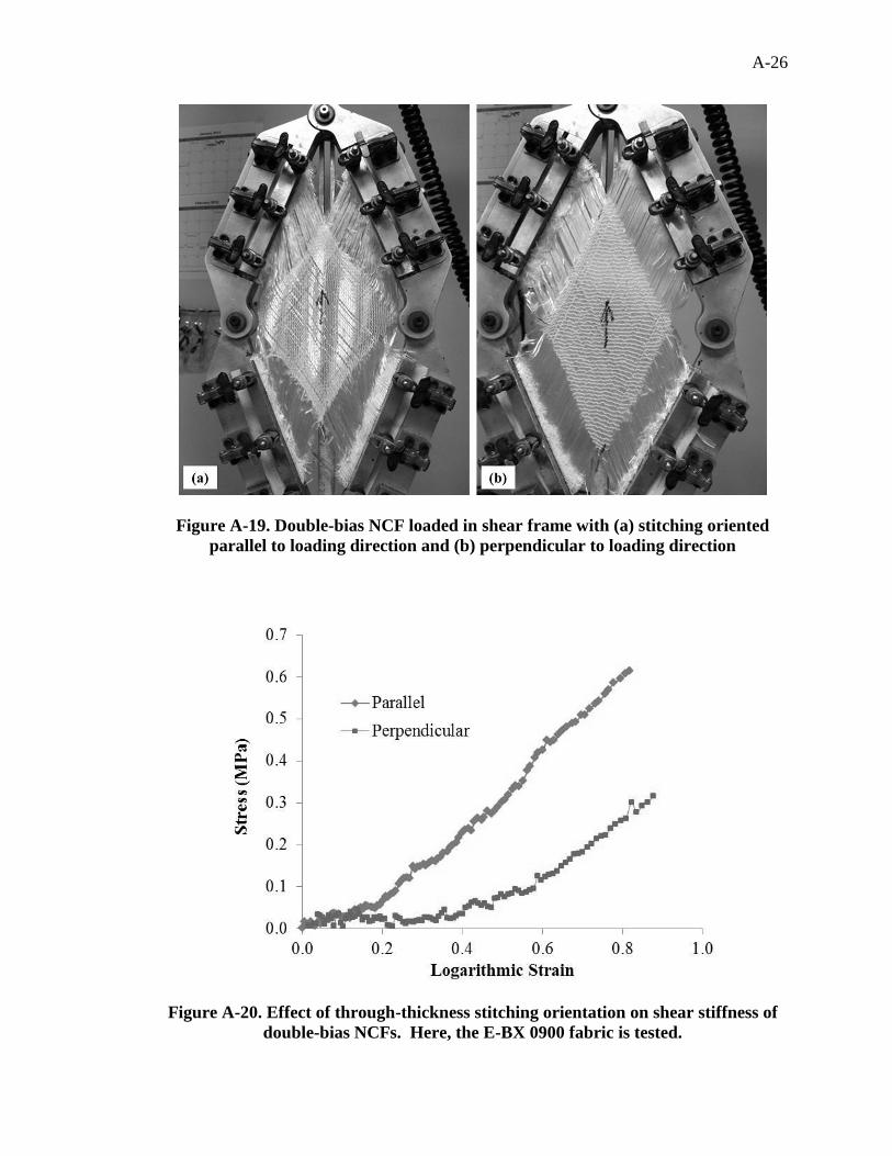
If the fabric is rotated such that the stitching is oriented perpendicular to the

loading direction as indicated by the arrow in Figure A-19, the stitching compresses with

the sample and therefore allows the yarns to rotate freely relative to each other, much like

they do in the case of the biaxial NCF. As a result, very little out-of-plane deformation is

observed (Figure A-19b), and the resulting shear stiffness is significantly lower than in

the case of the stitching being oriented parallel to the loading direction (Figure A-20).

A-26

Figure A-19. Double-bias NCF loaded in shear frame with (a) stitching oriented

parallel to loading direction and (b) perpendicular to loading direction

Figure A-20. Effect of through-thickness stitching orientation on shear stiffness of

double-bias NCFs. Here, the E-BX 0900 fabric is tested.

A-27

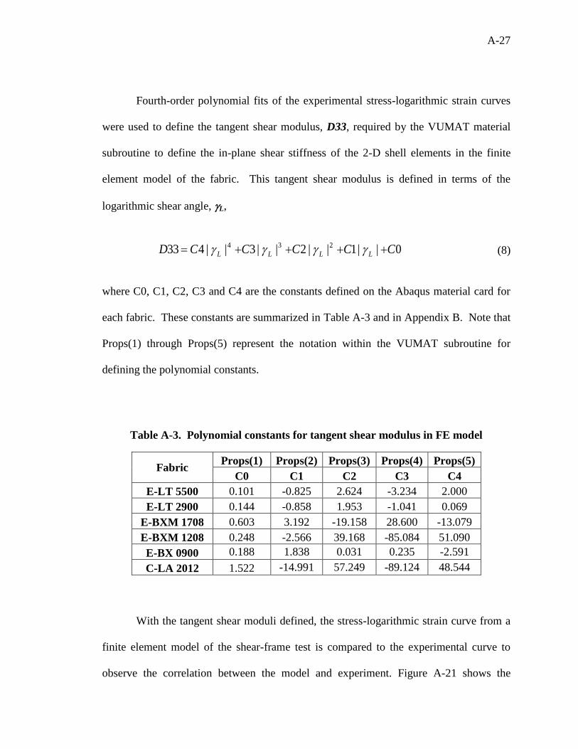
Fourth-order polynomial fits of the experimental stress-logarithmic strain curves

were used to define the tangent shear modulus, D33, required by the VUMAT material

subroutine to define the in-plane shear stiffness of the 2-D shell elements in the finite

element model of the fabric. This tangent shear modulus is defined in terms of the

logarithmic shear angle, L,

0||1||2||3||433 234 CCCCCD LLLL (8)

where C0, C1, C2, C3 and C4 are the constants defined on the Abaqus material card for

each fabric. These constants are summarized in Table A-3 and in Appendix B. Note that

Props(1) through Props(5) represent the notation within the VUMAT subroutine for

defining the polynomial constants.

Table A-3. Polynomial constants for tangent shear modulus in FE model

Fabric Props(1) Props(2) Props(3) Props(4) Props(5)

C0 C1 C2 C3 C4

E-LT 5500 0.101 -0.825 2.624 -3.234 2.000

E-LT 2900 0.144 -0.858 1.953 -1.041 0.069

E-BXM 1708 0.603 3.192 -19.158 28.600 -13.079

E-BXM 1208 0.248 -2.566 39.168 -85.084 51.090

E-BX 0900 0.188 1.838 0.031 0.235 -2.591

C-LA 2012 1.522 -14.991 57.249 -89.124 48.544

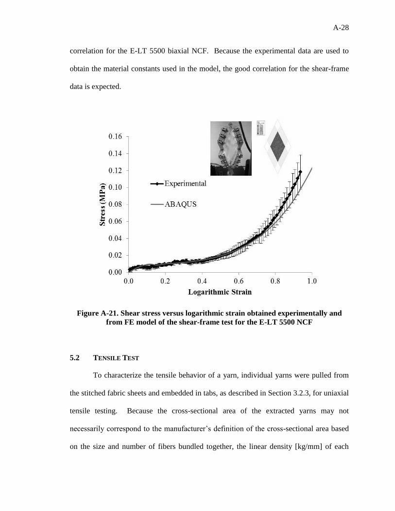
With the tangent shear moduli defined, the stress-logarithmic strain curve from a

finite element model of the shear-frame test is compared to the experimental curve to

observe the correlation between the model and experiment. Figure A-21 shows the

A-28

correlation for the E-LT 5500 biaxial NCF. Because the experimental data are used to

obtain the material constants used in the model, the good correlation for the shear-frame

data is expected.

Figure A-21. Shear stress versus logarithmic strain obtained experimentally and

from FE model of the shear-frame test for the E-LT 5500 NCF

5.2 TENSILE TEST

To characterize the tensile behavior of a yarn, individual yarns were pulled from

the stitched fabric sheets and embedded in tabs, as described in Section 3.2.3, for uniaxial

tensile testing. Because the cross-sectional area of the extracted yarns may not

necessarily correspond to the manufacturer’s definition of the cross-sectional area based

on the size and number of fibers bundled together, the linear density [kg/mm] of each

A-29

yarn was determined by measuring the mass and the length. This linear density was then

divided by the density of the material [kg/mm3] (Equation 3) to obtain the cross-sectional

area.

The measured uniaxial loads were divided by the cross-sectional area of each yarn

to determine the tensile stress. Similar to the case of the 2-D shell elements, the VUMAT

subroutine requires a tangent modulus, D11, for the 1-D beam elements to define the

tensile stiffness. This modulus is essentially the effective elastic modulus of the yarn for

that strain, taken from the slope of a linear regression of the experimental stress-true-

strain data.

Because all of the fabrics except the carbon unidirectional are made of E-glass

material, it was expected that the tensile modulus of the glass fabric yarns would be very

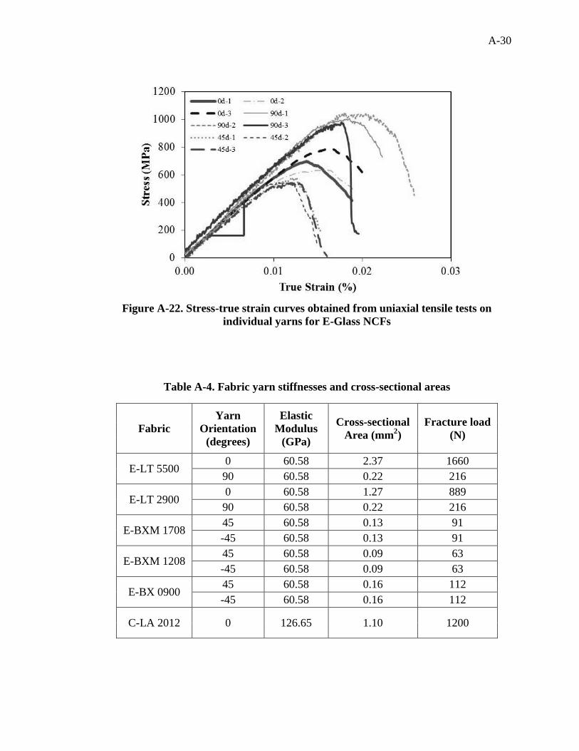
similar. Figure A-22 confirms this expectation that the slopes of the stress-true strain

curves from several different E-Glass NCFs are similar. Thus, the moduli were averaged

and found to be 60.58 GPa, which falls within the range of typical values for E-Glass

yarns [12]. For the carbon yarns (C-LA 2012 fabric), the elastic modulus was determined

to be 126.65 GPa, which also compares well to typical values [13]. The yarn moduli and

their respective cross sectional areas and fracture loads are summarized in Table A-4.

A-30

Figure A-22. Stress-true strain curves obtained from uniaxial tensile tests on

individual yarns for E-Glass NCFs

Table A-4. Fabric yarn stiffnesses and cross-sectional areas

Fabric

Yarn

Orientation

(degrees)

Elastic

Modulus

(GPa)

Cross-sectional

Area (mm2)

Fracture load

(N)

E-LT 5500 0 60.58 2.37 1660

90 60.58 0.22 216

E-LT 2900 0 60.58 1.27 889

90 60.58 0.22 216

E-BXM 1708 45 60.58 0.13 91

-45 60.58 0.13 91

E-BXM 1208 45 60.58 0.09 63

-45 60.58 0.09 63

E-BX 0900 45 60.58 0.16 112

-45 60.58 0.16 112

C-LA 2012 0 126.65 1.10 1200

A-31

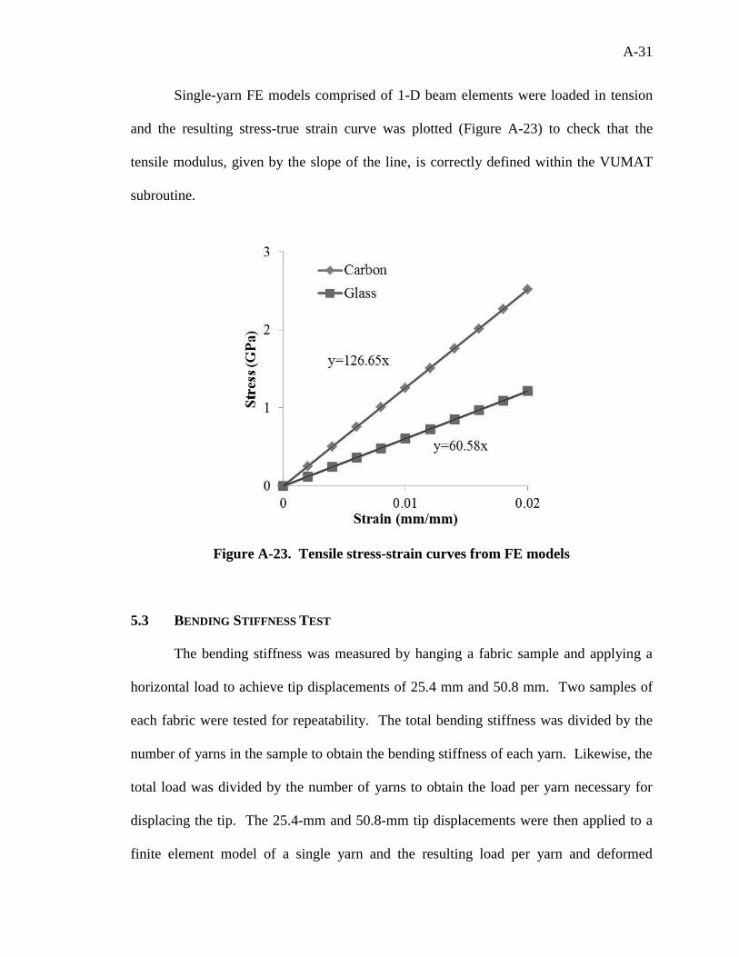
Single-yarn FE models comprised of 1-D beam elements were loaded in tension

and the resulting stress-true strain curve was plotted (Figure A-23) to check that the

tensile modulus, given by the slope of the line, is correctly defined within the VUMAT

subroutine.

Figure A-23. Tensile stress-strain curves from FE models

5.3 BENDING STIFFNESS TEST

The bending stiffness was measured by hanging a fabric sample and applying a

horizontal load to achieve tip displacements of 25.4 mm and 50.8 mm. Two samples of

each fabric were tested for repeatability. The total bending stiffness was divided by the

number of yarns in the sample to obtain the bending stiffness of each yarn. Likewise, the

total load was divided by the number of yarns to obtain the load per yarn necessary for

displacing the tip. The 25.4-mm and 50.8-mm tip displacements were then applied to a

finite element model of a single yarn and the resulting load per yarn and deformed

A-32

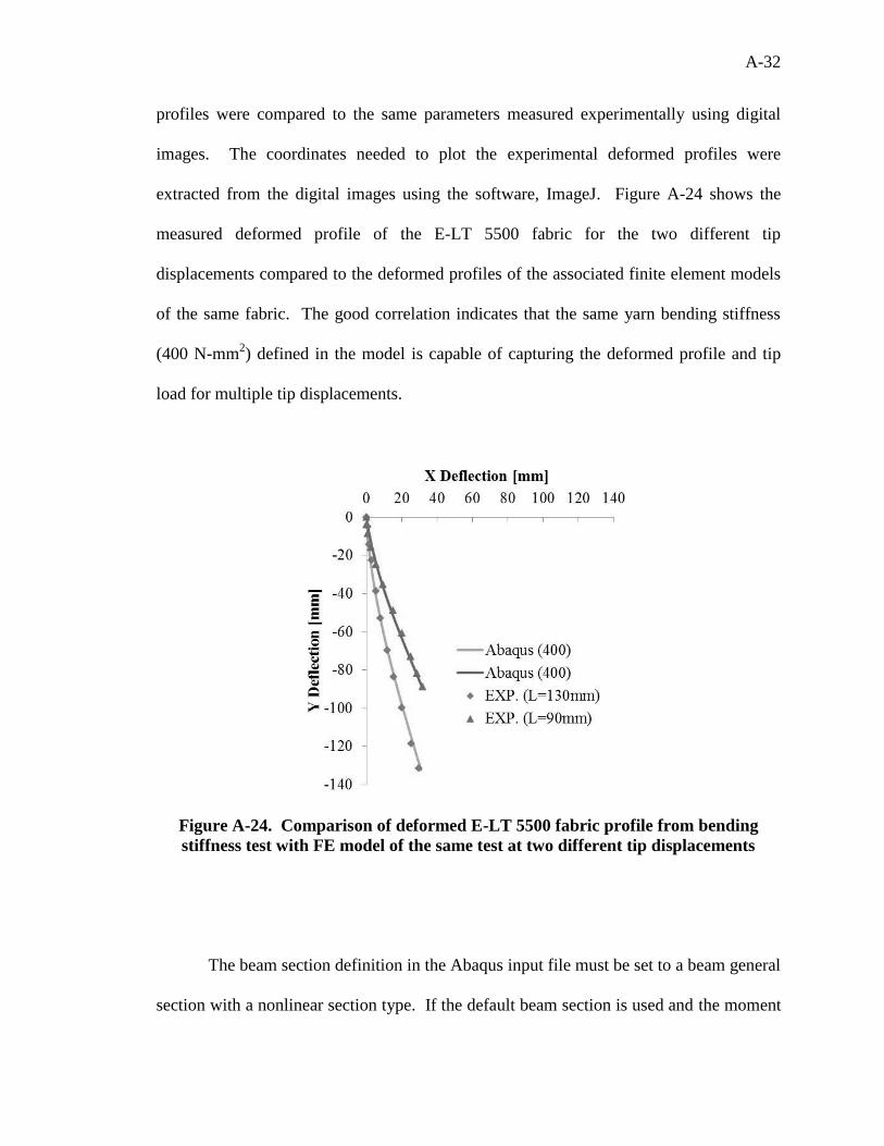
profiles were compared to the same parameters measured experimentally using digital

images. The coordinates needed to plot the experimental deformed profiles were

extracted from the digital images using the software, ImageJ. Figure A-24 shows the

measured deformed profile of the E-LT 5500 fabric for the two different tip

displacements compared to the deformed profiles of the associated finite element models

of the same fabric. The good correlation indicates that the same yarn bending stiffness

(400 N-mm2) defined in the model is capable of capturing the deformed profile and tip

load for multiple tip displacements.

Figure A-24. Comparison of deformed E-LT 5500 fabric profile from bending

stiffness test with FE model of the same test at two different tip displacements

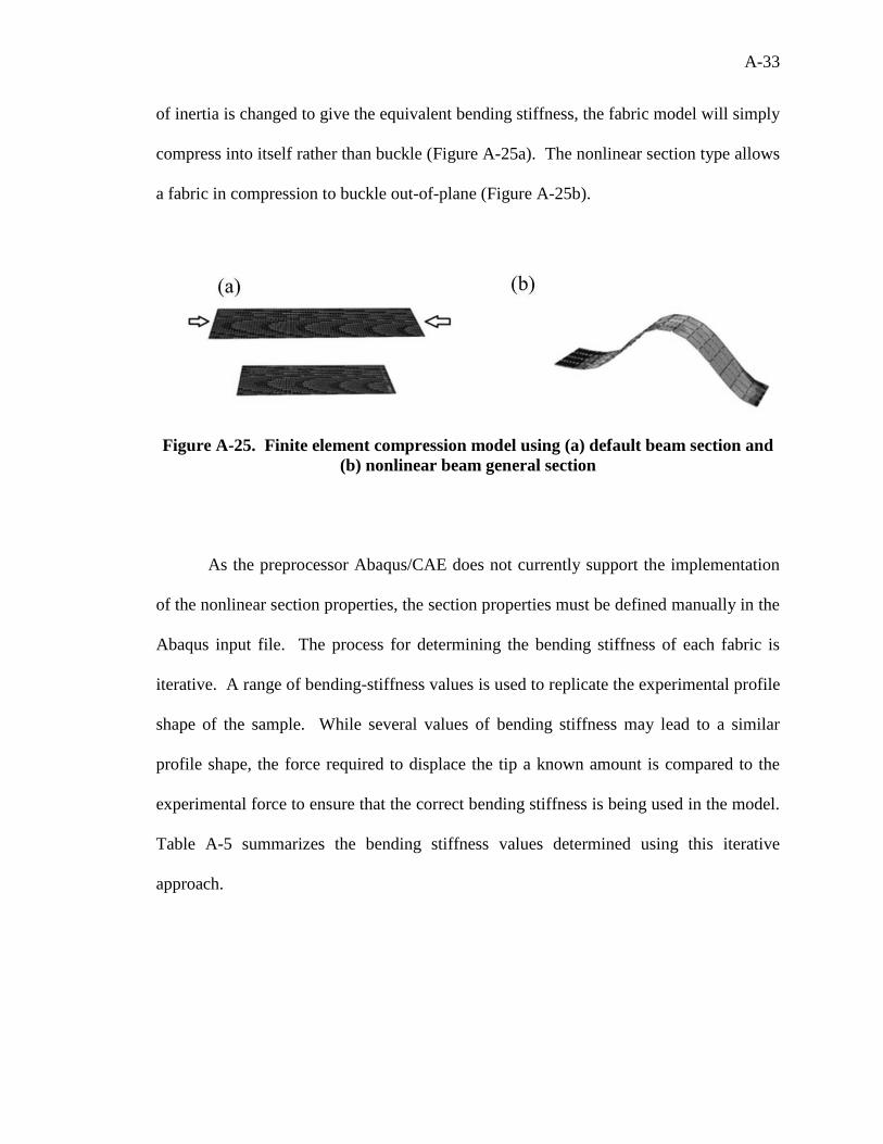
The beam section definition in the Abaqus input file must be set to a beam general

section with a nonlinear section type. If the default beam section is used and the moment

A-33

of inertia is changed to give the equivalent bending stiffness, the fabric model will simply

compress into itself rather than buckle (Figure A-25a). The nonlinear section type allows

a fabric in compression to buckle out-of-plane (Figure A-25b).

Figure A-25. Finite element compression model using (a) default beam section and

(b) nonlinear beam general section

As the preprocessor Abaqus/CAE does not currently support the implementation

of the nonlinear section properties, the section properties must be defined manually in the

Abaqus input file. The process for determining the bending stiffness of each fabric is

iterative. A range of bending-stiffness values is used to replicate the experimental profile

shape of the sample. While several values of bending stiffness may lead to a similar

profile shape, the force required to displace the tip a known amount is compared to the

experimental force to ensure that the correct bending stiffness is being used in the model.

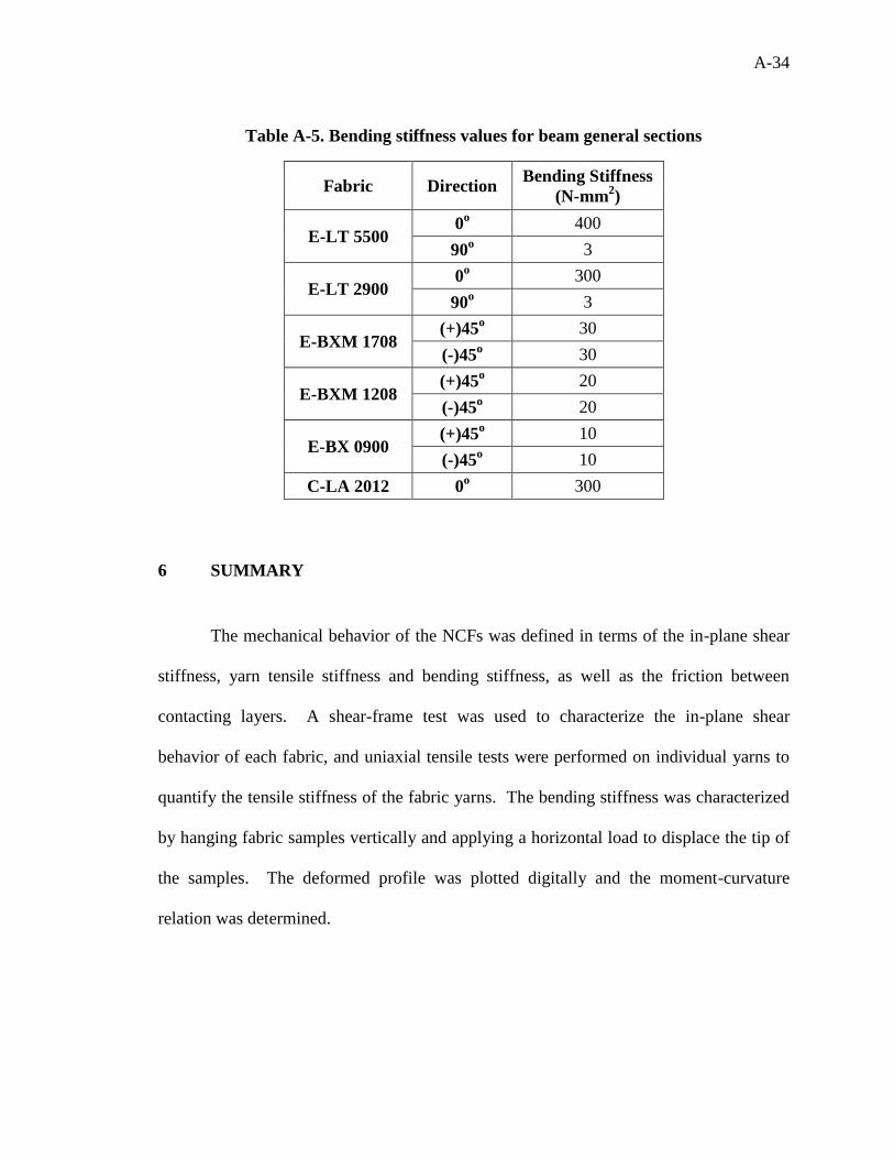
Table A-5 summarizes the bending stiffness values determined using this iterative

approach.

A-34

Table A-5. Bending stiffness values for beam general sections

Fabric Direction Bending Stiffness

(N-mm2)

E-LT 5500 0

o 400

90o 3

E-LT 2900 0

o 300

90o 3

E-BXM 1708 (+)45

o 30

(-)45o 30

E-BXM 1208 (+)45

o 20

(-)45o 20

E-BX 0900 (+)45

o 10

(-)45o 10

C-LA 2012 0o 300

6 SUMMARY

The mechanical behavior of the NCFs was defined in terms of the in-plane shear

stiffness, yarn tensile stiffness and bending stiffness, as well as the friction between

contacting layers. A shear-frame test was used to characterize the in-plane shear

behavior of each fabric, and uniaxial tensile tests were performed on individual yarns to

quantify the tensile stiffness of the fabric yarns. The bending stiffness was characterized

by hanging fabric samples vertically and applying a horizontal load to displace the tip of

the samples. The deformed profile was plotted digitally and the moment-curvature

relation was determined.

A-35

LITERATURE CITED

[1] Li, Xiang.: “Material Characterization of Woven-Fabric Composites and Finite

Element Analysis of the Thermostamping Process”, D.Eng. Dissertation, Dept. of

Mechanical Engineering, University of Massachusetts Lowell, 2005.

[2] Jauffrès, D., Sherwood, J.A., Morris, C.D., and Chen, J.: “Discrete mesoscopic

modelling for the simulation of woven-fabric reinforcement forming”, International

Journal of Material Forming, 2009.

[3] Fetfatsidis, K.A., Gamache, L., Sherwood, J.A., Jauffrès, D., and Chen J.: “Design

of an apparatus for measuring tool/fabric and fabric/fabric friction of woven-fabric

composites during the thermostamping process”. International Journal of Material

Forming (Accepted for Publication), 2011.

[4] Cao J., Akkerman R., Boisse P., Chen J., Cheng H. S., DeGraaf E. F., Gorczyca J.,

Harrison P., Hivet G., Launay J., Lee W., Liu L., Lomov S., Long A., Deluycker E.,

Morestin F., Padvoiskis J., Peng X. Q., Sherwood J., Stoilova T., Tao X. M.,

Verpoest I., Willems A., Wiggers J., Yu T. X., Zhu B.: Characterization of

mechanical behavior of woven fabrics: experimental methods and benchmark

results. Composites: Part A, 39:1037-1053, 2008.

[5] Jauffres D., Morris C. D., Sherwood J., Chen J. Simulation of the thermostamping of

woven composites: determination of the tensile and in-plane shearing behaviors.

12th ESAFORM Conference. Twente, Nederlands, 2009.

[6] Lomov S., Boisse P., Deluycker E., Morestin F., Vanclooster K., Vandepitte D.,

Verpoest I., Willems A.: Full-field strain measurements in textile deformability

studies. Composites: Part A, 39:1232-1244, 2008.

[7] Petrov, A.S., Sherwood, J.A., Fetfatsidis, K.A.: “Characterization and Finite Element

Modeling of Unidirectional Non-Crimp Fabric for Composite Manufacturing”,

Proceedings of the 15th

ESAFORM Conference, Erlangen, Germany, 2012.

[8] Lomov S., Willems A., Verpoest I., Zhu Y., Barburski M., Stoilova T.: Picture frame

test of woven composite reinforcements with full-field strain registration. Textile

Research Journal, 76:243-252, 2006.

[9] Boisse, P., Hamila, N., Vidal- Sallé, E., Dumont, F.: “Simulation of wrinkling during

textile composite reinforcement forming. Influence of tensile, in-plane shear and

A-36

bending stiffnesses”, Composites Sci. and Tech., 10.1016/j.compscitech.2011.01.011

(2010).

[10] de Bilbao, E., Soulat, D., Hivet, G., and Gasser, A.: Experimental Study of Bending

Behaviour of Reinforcements. Experimental Mechanics, March 2009.

[11] Soteropoulos, D., Fetfatsidis, K., Sherwood, J., and Langworthy, J.: “Digital Method

of Analyzing the Bending Stiffness of Non-Crimp Fabrics”, Proceedings of the 14th

ESAFORM Conference, Belfast, United Kingdom, 2011.

[12] The Engineering Toolbox

http://www.engineeringtoolbox.com/young-modulus-d_417.html (last checked April

9, 2012)

[13] Performance Composites, Ltd.

http://www.performance-composites.com/carbonfibre/mechanicalproperties_2.asp

(last checked April 9, 2012)