Appendix AAnswers to End-of-Chapter PracticeProblems

Chapter 1: Practice Problem #1 Answer (see Fig. A.1)

Fig. A.1 Answer to Chap. 1 Practice problem #1

T. J. Quirk et al., Excel 2010 for Biological and Life Sciences Statistics,DOI: 10.1007/978-1-4614-5779-4,� Springer Science+Business Media New York 2013

181

Chapter 1: Practice Problem #2 Answer (see Fig. A.2)

182 Appendix A: Answers to End-of-Chapter Practice Problems

Fig. A.2 Answer to Chap. 1 Practice problem #2

Chapter 1: Practice Problem #3 Answer (see Fig. A.3)

Appendix A: Answers to End-of-Chapter Practice Problems 183

Fig. A.3 Answer to Chap. 1 Practice problem #3

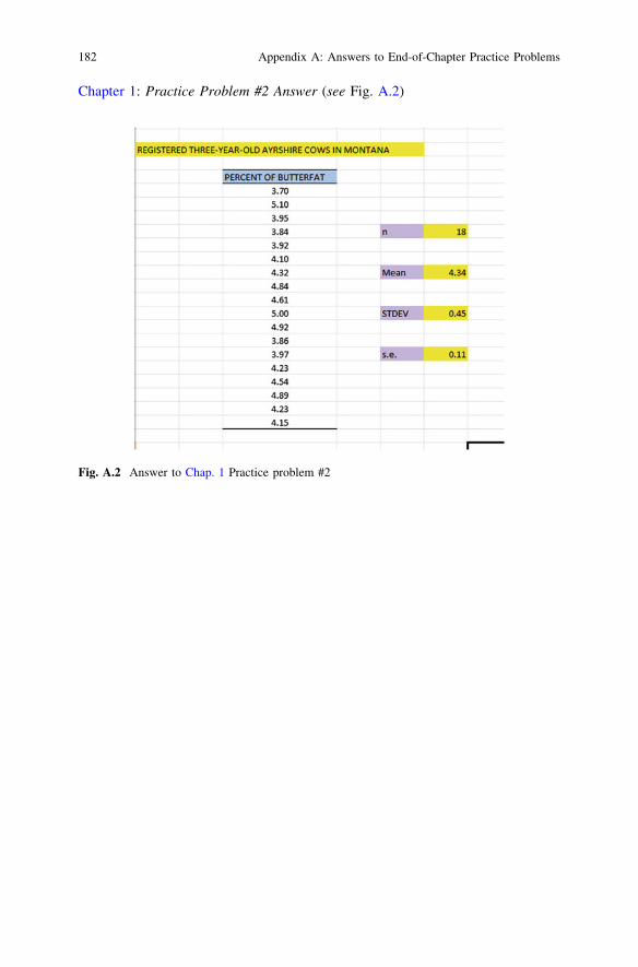
Chapter 2: Practice Problem #1 Answer (see Fig. A.4)

184 Appendix A: Answers to End-of-Chapter Practice Problems

Fig. A.4 Answer to Chap. 2 Practice problem #1

Chapter 2: Practice Problem #2 Answer (see Fig. A.5)

Appendix A: Answers to End-of-Chapter Practice Problems 185

Fig. A.5 Answer to Chap. 2 Practice problem #2

Chapter 2: Practice Problem #3 Answer (see Fig. A.6)

186 Appendix A: Answers to End-of-Chapter Practice Problems

Fig. A.6 Answer to Chap. 2 Practice problem #3

Chapter 3: Practice Problem #1 Answer (see Fig. A.7)

Appendix A: Answers to End-of-Chapter Practice Problems 187

Fig. A.7 Answer to Chap. 3 Practice problem #1

Chapter 3: Practice Problem #2 Answer (see Fig. A.8)

188 Appendix A: Answers to End-of-Chapter Practice Problems

Fig. A.8 Answer to Chap. 3 Practice problem #2

Chapter 3: Practice Problem #3 Answer (see Fig. A.9)

Appendix A: Answers to End-of-Chapter Practice Problems 189

Fig. A.9 Answer to Chap. 3 Practice problem #3

Chapter 4: Practice Problem #1 Answer (see Fig. A.10)

190 Appendix A: Answers to End-of-Chapter Practice Problems

Fig. A.10 Answer to Chap. 4 Practice problem #1

Chapter 4: Practice Problem #2 Answer (see Fig. A.11)

Appendix A: Answers to End-of-Chapter Practice Problems 191

Fig. A.11 Answer to Chap. 4 Practice problem #2

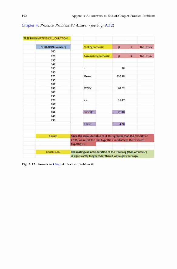
Chapter 4: Practice Problem #3 Answer (see Fig. A.12)

192 Appendix A: Answers to End-of-Chapter Practice Problems

Fig. A.12 Answer to Chap. 4 Practice problem #3

Chapter 5: Practice Problem #1 Answer (see Fig. A.13)

Appendix A: Answers to End-of-Chapter Practice Problems 193

Fig. A.13 Answer to Chap. 5 Practice problem #1

Chapter 5: Practice Problem #2 Answer (see Fig. A.14)

194 Appendix A: Answers to End-of-Chapter Practice Problems

Fig. A.14 Answer to Chap. 5 Practice problem #2

Chapter 5: Practice Problem #3 Answer (see Fig. A.15)

Appendix A: Answers to End-of-Chapter Practice Problems 195

Fig. A.15 Answer to Chap. 5 Practice problem #3

Chapter 6: Practice Problem #1 Answer (see Fig. A.16)

196 Appendix A: Answers to End-of-Chapter Practice Problems

Fig. A.16 Answer to Chap. 6 Practice problem #1

Chapter 6: Practice Problem #1 (continued)

1. r = +0.932. a = y-intercept = -0.0993. b = slope = 0.7654. Y = a + b X

Y = -0.099 + 0.765 X

5. Y = -0.099 + 0.765 (20)

Y = -0.099 + 15.3Y = 15.2 growth rings

Chapter 6: Practice Problem #2 Answer (see Fig. A.17)

Appendix A: Answers to End-of-Chapter Practice Problems 197

Fig. A.17 Answer to Chap. 6 Practice problem #2

198 Appendix A: Answers to End-of-Chapter Practice Problems

Chapter 6: Practice Problem #2 (continued)(2b) about 290 mg

1. r = +0.872. a = y-intercept = -8.283. b = slope = 14.584. Y = a + b X

Y = -8.28 + 14.58 X

5. Y = -8.28 + 14.58 (15)

Y = -8.28 + 218.7Y = 210.42 mg

Chapter 6: Practice Problem #3 Answer (see Fig. A.18)Chapter 6: Practice Problem #3 (continued)

1. r = +0.982. a = y-intercept = -1.3733. b = slope = 1.0204. Y = a + b X

Y = -1.373 + 1.020 X

5. Y = -1.373 + 1.020 (6.50)

Y = -1.373 + 6.630Y = 5.26 mm

Chapter 7: Practice Problem #1 Answer (see Fig. A.19)Chapter 7: Practice Problem #1 (continued)

1. Multiple correlation = 0.932. y-intercept = 0.56823. b1 = -0.00044. b2 = 0.00225. b3 = 0.05016. b4 = 0.00247. Y = a + b1 X 1 + b2 X2 + b3 X3 + b4 X4

Y = 0.5682 - 0.0004 X1 + 0.0022 X2 + 0.0501 X3 + 0.0024 X4

8. Y = 0.5682 - 0.0004 (610) + 0.0022 (550) + 0.0501 (3) + 0.0024 (610)

Y = 0.5682 - 0.244 + 1.21 + 0.150 + 1.464Y = 3.392 - 0.244Y = 3.15

9. 0.7910. 0.8711. 0.8312. 0.89

13. 0.7414. 0.7615. The best predictor of FIRST-YEAR GPA was GRE BIOLOGY (r = +0.89).16. The four predictors combined predict the FIRST-YEAR GPA at Rxy = 0.93,

and this is much better than the best single predictor by itself.

Fig. A.18 Answer to Chap. 6 Practice problem #3

Appendix A: Answers to End-of-Chapter Practice Problems 199

Chapter 7: Practice Problem #2 Answer (see Fig. A.20)Chapter 7: Practice Problem #2 (continued)

1. Rxy = 0.652. a = y-intercept = 322.2463. b1 = 1.044. b2 = 9.0055. Y = a + b1 X1 + b2 X2

Y = 322.246 + 1.04 X1 + 9.005 X2

6. Y = 322.246 + 1.04 (300) + 9.005 (2)

Y = 322.246 + 312 + 18.01Y = 652 g/meter squared/year

Fig. A.19 Answer to Chap. 7 Practice problem #1

200 Appendix A: Answers to End-of-Chapter Practice Problems

7. +0.628. +0.289. +0.14

10. Mean annual precipitation is the better predictor of productivity (r = +0.62)11. The two predictors combined predict productivity slightly better (Rxy = 0.65)

than the better single predictor by itself.

Chapter 7: Practice Problem #3 Answer (see Fig. A.21)Chapter 7: Practice Problem #3 (continued)

1. Multiple correlation = +0.952. a = y-intercept = -0.6843. b1 = -0.0034. b2 = 0.0025. b3 = 1.3786. b4 = -0.0487. Y = a + b1 X1 + b2 X2 + b3 X3 + b4 X4

Y = -0.684 - 0.003 X1 + 0.002 X2 + 1.378 X3 - 0.048 X4

8. Y = -0.684 - 0.003 (650) + 0.002 (630) + 1.378 (3.47) - 0.048 (4)

Fig. A.20 Answer to Chap. 7 Practice problem #2

Appendix A: Answers to End-of-Chapter Practice Problems 201

Y = -0.684 - 1.95 + 1.26 + 4.78 - 0.19Y = 6.04 - 2.824Y = 3.22

9. +0.5910. +0.6111. +0.8812. +0.4713. +0.80

Fig. A.21 Answer to Chap. 7 Practice problem #3

202 Appendix A: Answers to End-of-Chapter Practice Problems

14. +0.6115. +0.7116. +0.6517. The best single predictor of FROSH GPA was HS GPA (r = 0.88).18. The four predictors combined predict FROSH GPA at Rxy = 0.95, and this is

much better than the best single predictor by itself.

Chapter 8: Practice Problem #1 Answer (see Fig. A.22)Chapter 8: Practice Problem #1 (continued)

Let Group 1 = No Nitrogen, Group 2 = Low Nitrogen, and Group 3 = HighNitrogen

Appendix A: Answers to End-of-Chapter Practice Problems 203

Fig. A.22 Answer to Chap. 8 Practice problem #1

1. H0: l1 = l2 = l3

H1: l1 = l2 = l3

2. MSb = 2,322,790.773. MSw = 61,350.204. F = 2,322,790/61,350 = 37.865. critical F = 3.346. Result: Since 37.86 is greater than 3.34, we reject the null hypothesis and

accept the research hypothesis.7. There was a significant difference in the weight of the Daisy Fleabane between

the three treatments.

TREATMENT 2 vs. TREATMENT 3

8. H0: l2 = l3

H1: l2 = l3

9. 65510. 1416.6711. df = 31 - 3 = 2812. critical t = 2.04813. 1/10 + 1/12 = 0.10 + 0.08 = 0.18

s.e. = SQRT (61,350.20 * 0.18) = SQRT (11,043.04) = 105.086

14. ANOVA t = (655 - 1416.67)/105.086 = -761.67/105.086 = -7.2515. Result: Since the absolute value of -7.25 is greater than 2.048, we reject the

null hypothesis and accept the research hypothesis.16. Conclusion: Daisy Fleabane flowers weighed significantly more when the soil

contained high Nitrogen than when the soil contained low Nitrogen (1417 mgvs. 655 mg).

Chapter 8: Practice Problem #2 Answer (see Fig. A.23)Chapter 8: Practice Problem #2 (continued)

1. Null hypothesis: lA = lB = lC = lD

Research hypothesis: lA = lB = lC = lD

2. MSb = 0.723. MSw = 0.204. F = 0.72/0.20 = 3.605. critical F = 2.856. Since the F-value of 3.60 is greater than the critical F value of 2.85, we reject

the null hypothesis and accept the research hypothesis.7. There was a significant difference in cumulative GPA between the four groups

of students in their reasons for taking Introductory Biology.8. Null hypothesis: lA = lC

204 Appendix A: Answers to End-of-Chapter Practice Problems

Research hypothesis: lA = lC

9. 3.4010. 3.1211. degrees of freedom = 42 - 4 = 3812. critical t = 2.02413. s.e. ANOVA = SQRT(MSw x {1/10 + 1/11}) = SQRT (0.20 9 0.19) =

SQRT (0.038) = 0.20

14. ANOVA t = (3.40 - 3.12)/0.20 = 1.4215. Since the absolute value of 1.42 is LESS than the critical t of 2.024, we accept

the null hypothesis.16. There was no difference in cumulative GPA between Premed students and

Other Science majors in their reasons for taking the Introductory Biologycourse.

Fig. A.23 Answer to Chap. 8 Practice problem #2

Appendix A: Answers to End-of-Chapter Practice Problems 205

Chapter 8: Practice Problem #3 Answer (see Fig. A.24)

206 Appendix A: Answers to End-of-Chapter Practice Problems

Fig. A.24 Answer to Chap. 8 Practice problem #3

Chapter 8: Practice Problem #3 (continued)

Let 200 fish = Group 1, 350 fish = Group 2, 500 fish = Group 3, and700 fish = Group 4

1. Null hypothesis: l1 ¼ l2 ¼ l3 ¼ l4

Research hypothesis: l1 6¼ l2 6¼ l3 6¼ l4

2. MSb = 4.303. MSw = 0.044. F = 4.30/0.04 = 107.505. critical F = 2.816. Result: Since the F-value of 107.50 is greater than the critical F value of 2.81,

we reject the null hypothesis and accept the research hypothesis.7. Conclusion: There was a significant difference between the four types of

crowding conditions in the weight of the brown trout.8. Null hypothesis: l2 ¼ l3

Research hypothesis: l2 6¼ l3

9. 3.77 g10. 2.74 g11. degrees of freedom = 50 - 4 = 4612. critical t = 1.9613. s.e. ANOVA = SQRT(MSw x {1/12 + 1/14}) = SQRT (0.04 9 0.15)

= SQRT (0.006) = 0.0814. ANOVA t = (3.77 - 2.74)/0.08 = 12.8815. Since the absolute value of 12.88 is greater than the critical t of 1.96, we reject

the null hypothesis and accept the research hypothesis.16. Brown trout raised in a container with 350 fish weighed significantly more

than brown trout raised in a container with 500 fish (3.77 g versus 2.74 g).

Appendix A: Answers to End-of-Chapter Practice Problems 207

Appendix BPractice Test

Chapter 1: Practice Test

Suppose that you were hired as a research assistant on a project involvinghummingbirds, and that your responsibility on this team was to measure the width(at the widest part) of hummingbird eggs (measured in millimeters). You want totry out your Excel skills on a small sample of eggs and measure them. Thehypothetical data is given below (see Fig. B.1).

Fig. B.1 Worksheet data for Chap. 1 practice test (Practical example)

T. J. Quirk et al., Excel 2010 for Biological and Life Sciences Statistics,DOI: 10.1007/978-1-4614-5779-4,� Springer Science+Business Media New York 2013

209

(a) Create an Excel table for these data, and then use Excel to the right of the tableto find the sample size, mean, standard deviation, and standard error of themean for these data. Label your answers, and round off the mean, standarddeviation, and standard error of the mean to two decimal places.

(b) Save the file as: eggs3

Chapter 2: Practice Test

Suppose that you were hired to test the fluoride levels in drinking water inJefferson County, Colorado. Historically, there are a total of 42 water samplecollection sites. Because of budget constraints, you need to choose a randomsample of 12 of these 42 water sample collection sites.

(a) Set up a spreadsheet of frame numbers for these water samples with theheading: FRAME NUMBERS.

(b) Then, create a separate column to the right of these frame numbers whichduplicates these frame numbers with the title: Duplicate frame numbers.

(c) Then, create a separate column to the right of these duplicate frame numberscalled RAND NO. and use the = RAND() function to assign random numbersto all of the frame numbers in the duplicate frame numbers column, and changethis column format so that 3 decimal places appear for each random number.

(d) Sort the duplicate frame numbers and random numbers into a random order.(e) Print the result so that the spreadsheet fits onto one page.(f) Circle on your printout the I.D. number of the first 12 water sample locations

that you would use in your test.(g) Save the file as: RAND15

Important note: Note that everyone who does this problem will generate adifferent random order of water sample sites ID numbers sinceExcel assign a different random number each time the RAND()command is used. For this reason, the answer to this problemgiven in this Excel Guide will have a completely differentsequence of random numbers from the random sequence thatyou generate. This is normal and what is to be expected.

Chapter 3: Practice Test

Suppose that you have been asked to analyze some environmental impact datafrom the state of Texas in terms of the amount of SO2 concentration in theatmosphere in different sites of Texas compared to three years ago to see if thisconcentration (and the air the people who live there breathe) has changed. SO2 ismeasured in parts per billion (ppb). Three years ago, when this research was lastdone, the average concentration of SO2 in these sites was 120 ppb. Since then, thestate has undertaken a comprehensive program to improve the air that people inthese sites breathe, and you have been asked to ‘‘run the data’’ to see if any changehas occurred.

210 Appendix B: Practice Test

Is the air that people breathe in these sites now different from the air that peoplebreathed three years ago? You have decided to test your Excel skills on a sampleof hypothetical data given in Fig. B.2

(a) Create an Excel table for these data, and use Excel to the right of the table tofind the sample size, mean, standard deviation, and standard error of the meanfor these data. Label your answers, and round off the mean, standard deviation,and standard error of the mean to two decimal places in number format.

(b) By hand, write the null hypothesis and the research hypothesis on yourprintout.

(c) Use Excel’s TINV function to find the 95 % confidence interval about the meanfor these data. Label your answers. Use two decimal places for the confidenceinterval figures in number format.

(d) On your printout, draw a diagram of this 95 % confidence interval by hand,including the reference value.

(e) On your spreadsheet, enter the result.(f) On your spreadsheet, enter the conclusion in plain English.(g) Print the data and the results so that your spreadsheet fits onto one page.(h) Save the file as: PARTS3

Fig. B.2 Worksheet data for Chap. 3 practice test (Practical example)

Appendix B: Practice Test 211

Chapter 4: Practice Test

Suppose that you wanted to measure the evolution of birds after a severeenvironmental change. Specifically, you want to study the effect of a severedrought with very little rainfall on the beak depth of finches on a small island in thePacific. Let’s suppose that the drought has lasted six years and that before thedrought, the average beak depth of finches on this island was 9.2 mm. Has the beakdepth of finches changed after this environmental challenge? You measure thebeak depth of a sample of finches, and the hypothetical data is given in Fig. B.3.

212 Appendix B: Practice Test

Fig. B.3 Worksheet data for Chap. 4 practice test (Practical example)

(a) Write the null hypothesis and the research hypothesis on your spreadsheet.(b) Create a spreadsheet for these data, and then use Excel to find the sample size,

mean, standard deviation, and standard error of the mean to the right of thedata set. Use number format (3 decimal places) for the mean, standarddeviation, and standard error of the mean.

(c) Type the critical t from the t-table in Appendix E onto your spreadsheet, andlabel it.

(d) Use Excel to compute the t test value for these data (use 3 decimal places) andlabel it on your spreadsheet.

(e) Type the result on your spreadsheet, and then type the conclusion in plainEnglish on your spreadsheet.

(f) Save the file as: beak3

Chapter 5: Practice Test

Suppose that you wanted to study the duration of hibernation of a species ofhedgehogs (Erinaceus europaeus) in two regions of the United States (NORTH vs.SOUTH). Suppose, further, that researchers have captured hedgehogs in theseregions, attached radio tags to their bodies, and then released them back into thesite where they were captured. The researchers monitored the movements of thehedgehogs during the winter months to determine the number of days that they didnot leave their nests. The researchers have selected a random sample of hedgehogsfrom each region, and you want to test your Excel skills on the hypothetical datagiven in Fig. B.4.

(a) Write the null hypothesis and the research hypothesis.(b) Create an Excel table that summarizes these data.(c) Use Excel to find the standard error of the difference of the means.(d) Use Excel to perform a two-group t-test. What is the value of t that you obtain

(use two decimal places)?(e) On your spreadsheet, type the critical value of t using the t-table in Appendix E.(f) Type the result of the test on your spreadsheet.(g) Type your conclusion in plain English on your spreadsheet.(h) Save the file as: HEDGE3(i) Print the final spreadsheet so that it fits onto one page.

Chapter 6: Practice Test

How does elevation effect overall plant height? Suppose that you wanted to studythis question using the height of yarrow plants. The plants were germinated fromseeds collected at different elevations from 15 different sites in the western UnitedStates. The plants were reared in a greenhouse to control for the effect oftemperature on plant height. The hypothetical data are given in Fig. B.5.

Create an Excel spreadsheet, and enter the data.

(a) Create an XY scatterplot of these two sets of data such that:

Appendix B: Practice Test 213

Fig. B.4 Worksheet data for Chap. 5 practice test (Practical example)

Fig. B.5 Worksheet data for Chap. 6 practice test (Practical example)

214 Appendix B: Practice Test

• top title: RELATIONSHIP BETWEEN ELEVATION AND HEIGHT OFYARROW PLANTS

• x-axis title: Elevation (m)• y-axis title: Height (cm)• move the chart below the table• re-size the chart so that it is 7 columns wide and 25 rows long• delete the legend• delete the gridlines

(b) Create the least-squares regression line for these data on the scatterplot.(c) Use Excel to run the regression statistics to find the equation for the least-

squares regression line for these data and display the results below the charton your spreadsheet. Add the regression equation to the chart. Use numberformat (3 decimal places) for the correlation and for the coefficients.

Print just the input data and the chart so that this information fits onto one pagein portrait format.

Then, print just the regression output table on a separate page so that it fits ontothat separate page in portrait format.By hand:

(d) Circle and label the value of the y-intercept and the slope of the regression lineon your printout.

(e) Write the regression equation by hand on your printout for these data (usethree decimal places for the y-intercept and the slope).

(f) Circle and label the correlation between the two sets of scores in the regressionanalysis summary output table on your printout.

(g) Underneath the regression equation you wrote by hand on your printout, usethe regression equation to predict the average height of the yarrow plant youwould predict for an elevation of 2000 m.

(h) Read from the graph, the average height of the yarrow plant you would predictfor an elevation of 2,500 m, and write your answer in the space immediatelybelow:

(i) save the file as: Yarrow3

Chapter 7: Practice Test

Suppose that you have been hired by the United States Department of Agriculture(USDA) to analyze corn yields from Iowa farms over one year (a single growingseason). Suppose, further, that these data will represent a pilot study that will beincluded in a larger ongoing analysis of corn yield in the Midwest. You want todetermine if you can predict the amount of corn produced in bushels per acre(bu/acre) based on three predictors: (1) water measured in inches of rainfall peryear (in/year), (2) fertilizer measured in the amount of nitrogen applied to the soilin pounds per acre (lbs/acre), and (3) average temperature during the growingseason measured in degrees Fahrenheit (�F).

Appendix B: Practice Test 215

To check your skills in Excel, you have selected a random sample of corn fromeach of eleven farms selected randomly and recorded the hypothetical given inFig. B.6.

(a) Create an Excel spreadsheet using YIELD as the criterion (Y), and the othervariables as the three predictors of this criterion (X1 = RAINFALL,X2 = NITROGEN, and X3 = TEMPERATURE).

(b) Use Excel’s multiple regression function to find the relationship between thesefour variables and place the SUMMARY OUTPUT below the table.

(c) Use number format (2 decimal places) for the multiple correlation on theSummary Output, and use two decimal places for the coefficients in theSUMMARY OUTPUT.

(d) Save the file as: yield15(e) Print the table and regression results below the table so that they fit onto one page.

Answer the following questions using your Excel printout:

1. What is the multiple correlation Rxy?2. What is the y-intercept a?3. What is the coefficient for RAINFALL b1?4. What is the coefficient for NITROGEN b2?5. What is the coefficient for TEMPERATURE b3?6. What is the multiple regression equation?7. Predict the corn yield you would expect for rainfall of 28 inches per year,

nitrogen at 205 pounds/acre, and temperature of 83 degrees Fahrenheit.(f) Now, go back to your Excel file and create a correlation matrix for these four

variables, and place it underneath the SUMMARY OUTPUT.(g) Re-save this file as: yield15(h) Now, print out just this correlation matrix on a separate sheet of paper.

216 Appendix B: Practice Test

Fig. B.6 Worksheet data for Chap. 7 practice test (Practical example)

Answer to the following questions using your Excel printout. (Be sure to includethe plus or minus sign for each correlation):

8. What is the correlation between RAINFALL and YIELD?9. What is the correlation between NITROGEN and YIELD?10. What is the correlation between TEMPERATURE and YIELD?11. What is the correlation between NITROGEN and RAINFALL?12. What is the correlation between TEMPERATURE and RAINFALL?13. What is the correlation between TEMPERATURE and NITROGEN?14. Discuss which of the three predictors is the best predictor of corn yield.15. Explain in words how much better the three predictor variables combined

predict corn yield than the best single predictor by itself.

Chapter 8: Practice Test

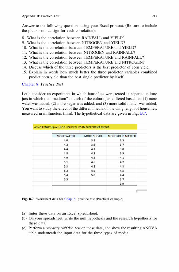
Let’s consider an experiment in which houseflies were reared in separate culturejars in which the ‘‘medium’’ in each of the culture jars differed based on: (1) morewater was added, (2) more sugar was added, and (3) more solid matter was added.You want to study the effect of the different media on the wing length of houseflies,measured in millimeters (mm). The hypothetical data are given in Fig. B.7.

(a) Enter these data on an Excel spreadsheet.(b) On your spreadsheet, write the null hypothesis and the research hypothesis for

these data.(c) Perform a one-way ANOVA test on these data, and show the resulting ANOVA

table underneath the input data for the three types of media.

Appendix B: Practice Test 217

Fig. B.7 Worksheet data for Chap. 8 practice test (Practical example)

(d) If the F-value in the ANOVA table is significant, create an Excel formula tocompute the ANOVA t-test comparing the more water added medium versusthe more solid matter added medium, and show the results below the ANOVAtable on the spreadsheet (put the standard error and the ANOVA t-test value onseparate lines of your spreadsheet, and use two decimal places for each value)

(e) Print out the resulting spreadsheet so that all of the information fits onto onepage.

(f) On your printout, label by hand the MS (between groups) and the MS (withingroups).

(g) Circle and label the value for F on your printout for the ANOVA of the inputdata.

(h) Label by hand on the printout the mean for more water added medium and themean for more solid matter added medium that were produced by yourANOVA formulas.

(i) Save the spreadsheet as: wing10

On a separate sheet of paper, now do the following by hand:

(j) find the critical value of F in the ANOVA Single Factor results table(k) write a summary of the result of the ANOVA test for the input data(l) write a summary of the conclusion of the ANOVA test in plain English for the

input data(m) write the null hypothesis and the research hypothesis comparing the more

water added medium versus the more solid matter added medium(n) compute the degrees of freedom for the ANOVA t-test by hand for three types

of media(o) use Excel to compute the standard error (s.e.) of the ANOVA t-test(p) Use Excel to compute the ANOVA t-test value(q) write the critical value of t for the ANOVA t-test using the table in Appendix E.(r) write a summary of the result of the ANOVA t-test(s) write a summary of the conclusion of the ANOVA t-test in plain English

ReferencesThere are no references at the end of the Practice Test.

218 Appendix B: Practice Test

Appendix CAnswers to Practice Test

Practice Test Answer: Chapter 1 (see. Fig. C.1)

Fig. C.1 Practice test answer to Chap. 1 problem

T. J. Quirk et al., Excel 2010 for Biological and Life Sciences Statistics,DOI: 10.1007/978-1-4614-5779-4,� Springer Science+Business Media New York 2013

219

Practice Test Answer: Chapter 2 (see. Fig. C.2)

Fig. C.2 Practice test answer to Chap. 2 problem

220 Appendix C: Answers to Practice Test

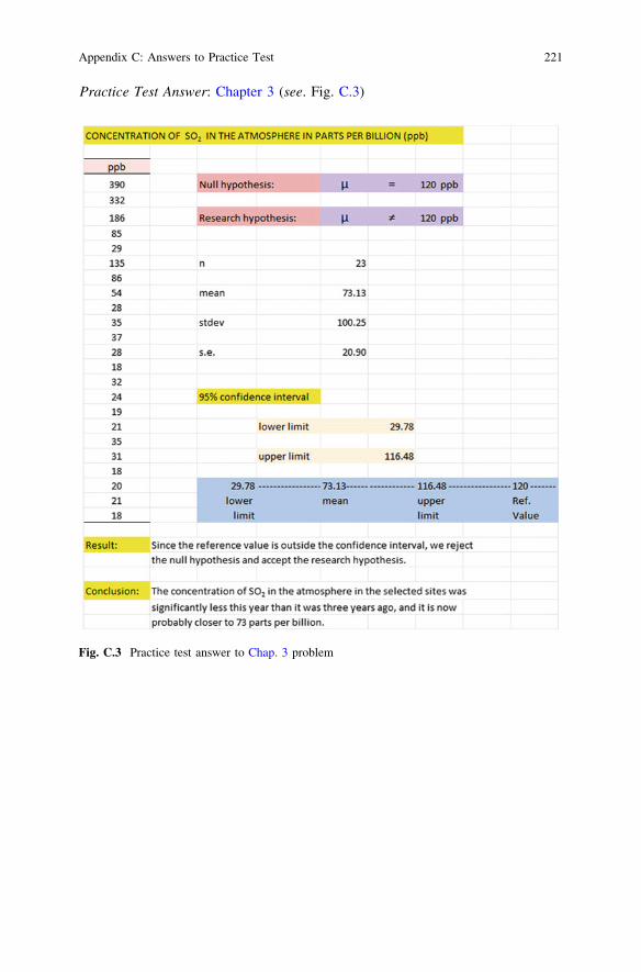
Practice Test Answer: Chapter 3 (see. Fig. C.3)

Appendix C: Answers to Practice Test 221

Fig. C.3 Practice test answer to Chap. 3 problem

Practice Test Answer: Chapter 4 (see. Fig. C.4)

222 Appendix C: Answers to Practice Test

Fig. C.4 Practice test answer to Chap. 4 problem

Practice Test Answer: Chapter 5 (see. Fig. C.5)

Appendix C: Answers to Practice Test 223

Fig. C.5 Practice test answer to Chap. 5 problem

Practice Test Answer: Chapter 6 (see. Fig. C.6)

224 Appendix C: Answers to Practice Test

Fig. C.6 Practice test answer to Chap. 6 problem

Practice Test Answer: Chapter 6 (continued)

(d) a = y-intercept = 111.293

b = slope = -0.035 (note the negative sign!)

(e) Y = a + b X

Y = 111.293 - 0.035 X

(f) r = correlation = -0.93 (note the negative sign!)(g) Y = 111.293 - 0.035 (2000)

Y = 111.293 - 70Y = 41.29 cm.

(h) About 23–25 cm.

Practice Test Answer: Chapter 7 (see. Fig. C.7)Practice Test Answer: Chapter 7 (continued)

1. Rxy = 0.782. a = y-intercept = 744.95

Appendix C: Answers to Practice Test 225

Fig. C.7 Practice test answer to Chap. 7 problem

3. b1 = 6.334. b2 = 0.515. b3 = -9.846. Y = a + b1 X1 + b2 X2 + b3 X3

Y = 744.95 + 6.33 X1 + 0.51 X2 - 9.84 X3

7. Y = 744.95 + 6.33 (28) + 0.51 (205) - 9.84 (83)

Y = 744.95 + 177.24 + 104.55 - 816.72Y = 1026.74 - 816.72Y = 210 bu/acre

8. +0.199. +0.31

10. -0.7011. +0.0312. +0.0013. -0.0514. The best predictor of corn yield was TEMPERATURE with a correlation of

-0.70. (Note: Remember to ignore the negative sign and just use 0.70.)15. The three predictors combined predict corn yield much better (Rxy = 0.78)

than the best single predictor by itself.

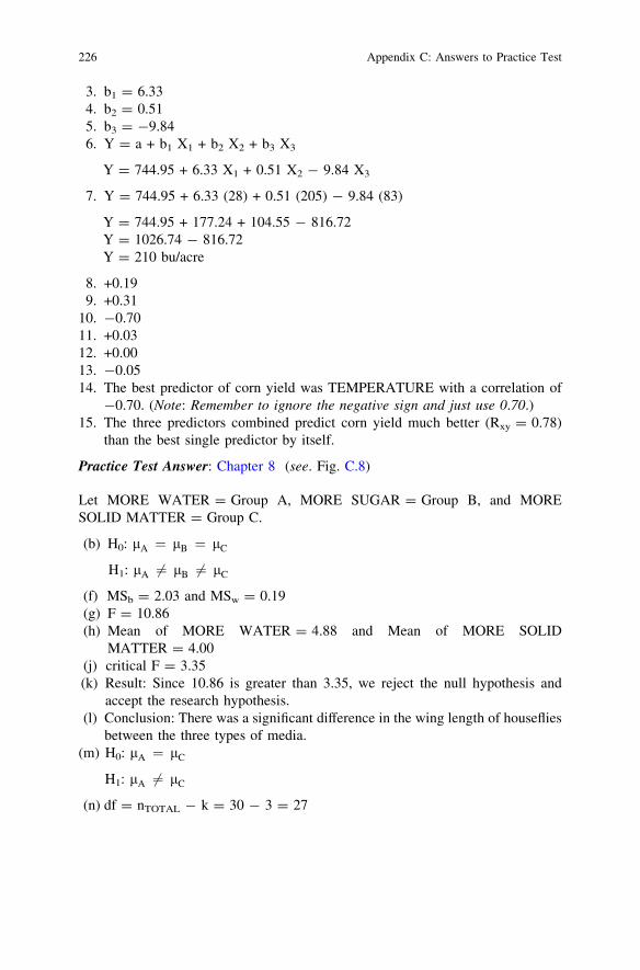
Practice Test Answer: Chapter 8 (see. Fig. C.8)

Let MORE WATER = Group A, MORE SUGAR = Group B, and MORESOLID MATTER = Group C.

(b) H0: lA ¼ lB ¼ lC

H1: lA 6¼ lB 6¼ lC

(f) MSb = 2.03 and MSw = 0.19(g) F = 10.86(h) Mean of MORE WATER = 4.88 and Mean of MORE SOLID

MATTER = 4.00(j) critical F = 3.35(k) Result: Since 10.86 is greater than 3.35, we reject the null hypothesis and

accept the research hypothesis.(l) Conclusion: There was a significant difference in the wing length of houseflies

between the three types of media.(m) H0: lA ¼ lC

H1: lA 6¼ lC

(n) df = nTOTAL - k = 30 - 3 = 27

226 Appendix C: Answers to Practice Test

Practice Test Answer: Chapter 8 (continued)

(o) 1/10 + 1/11 = 0.19

s.e = SQRT (0.19 * 0.19)s.e. = SQRT (0.036)s.e. = 0.19

(p) ANOVA t = (4.88 - 4.00)/0.19 = 4.66(q) critical t = 2.052(r) Result: Since the absolute value of 4.66 is greater than the critical t of 2.052,

we reject the null hypothesis and accept the research hypothesis.(s) Conclusion: The wing length of houseflies was significantly longer in the

MORE WATER ADDED medium than the MORE SOLID MATTERADDED medium (4.88 mm vs. 4.00 mm)

Fig. C.8 Practice test answer to Chap. 8 problem

Appendix C: Answers to Practice Test 227

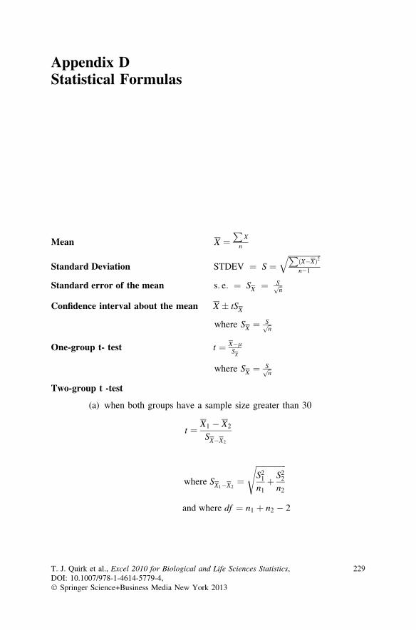
Appendix DStatistical Formulas

Mean X ¼P

X

n

Standard Deviation STDEV ¼ S ¼ffiffiffiffiffiffiffiffiffiffiffiffiffiffiffiffiffiPðX�XÞ2

n�1

q

Standard error of the mean s: e: ¼ SX ¼ Sffiffinp

Confidence interval about the mean X � tSX

where SX ¼ Sffiffinp

One-group t- test t ¼ X�lS

X

where SX ¼ Sffiffinp

Two-group t -test

(a) when both groups have a sample size greater than 30

t ¼ X1 � X2

SX�X2

where SX1�X2¼

ffiffiffiffiffiffiffiffiffiffiffiffiffiffiffiS2

1

n1þ S2

2

n2

s

and where df ¼ n1 þ n2 � 2

T. J. Quirk et al., Excel 2010 for Biological and Life Sciences Statistics,DOI: 10.1007/978-1-4614-5779-4,� Springer Science+Business Media New York 2013

229

(b) when one or both groups have a sample size less than 30

t ¼ X1 � X2

SX1�X2

where SX1�X2¼

ffiffiffiffiffiffiffiffiffiffiffiffiffiffiffiffiffiffiffiffiffiffiffiffiffiffiffiffiffiffiffiffiffiffiffiffiffiffiffiffiffiffiffiffiffiffiffiffiffiffiffiffiffiffiffiffiffiffiffiffiffiffiffiffiffiffiffiffiffiffin1 � 1ð ÞS2

1 þ n2 � 1ð ÞS22

n1 þ n2 � 21n1þ 1

n2

� �s

and where df ¼ n1 þ n2 � 2

Correlation r ¼1

n�1

PX�Xð ÞðY�YÞSxSy

where Sx = standard deviation of X

and where Sy = standard deviation of Y

Simple linear regression Y = a + b X

where a = y-intercept and b = slope of the line

Multiple regression equation Y = a + b1 X1 + b 2 X 2 + b 3 X 3 + etc.

where a = y-intercept

One-way ANOVA F-test F = MS b/MS w

ANOVA t test ANOVAt ¼ X1�X2s:e:ANOVA

where s:e:ANOVA ¼ffiffiffiffiffiffiffiffiffiffiffiffiffiffiffiffiffiffiffiffiffiffiffiffiffiffiffi

MSw1n1þ 1

n2

� �r

and where df ¼ nTOTAL � k

where nTOTAL = n1 + n2 + n3 + etc.

and where k = the number of groups

230 Appendix D: Statistical Formulas

Appendix Et-Table

Critical t-values needed for rejection of the null hypothesis (see Fig. E.1)

T. J. Quirk et al., Excel 2010 for Biological and Life Sciences Statistics,DOI: 10.1007/978-1-4614-5779-4,� Springer Science+Business Media New York 2013

231

Fig. E.1 Critical t-values needed for rejection of the null hypothesis

232 Appendix E: t-Table

Author’s Biography

At the beginning of his academic career, Prof. Quirk spent six years in educationalresearch at The American Institutes for Research and Educational Testing Service.He is currently a Professor of Marketing in the George Herbert Walker School ofBusiness & Technology at Webster University based in St. Louis, Missouri (USA)where he teaches Marketing Statistics, Marketing Research, and Pricing Strategies.He has written 60? textbook supplements in Marketing and Management,published 20? articles in professional journals, and presented 20? papers atprofessional meetings. He holds a B.S. in Mathematics from John CarrollUniversity, both an M.A. in Education and a Ph.D. in Educational Psychologyfrom Stanford University, and an M.B.A. from The University of Missouri-St.Louis. This is Professor Quirk’s seventh statistics book with Springer.

Meghan Quirk holds both a Ph.D. in Biological Education and an M.A. inBiological Sciences from the University of Northern Colorado (UNC) and a B.A.in Biology and Religion at Principia College in Elsah, Illinois. She has doneresearch on foodweb dynamics at Wind Cave National Park in South Dakota andresearch in agro-ecology in Southern Belize. She has co-authored an article onshortgrass steppe ecosystems in Photochemistry & Photobiology and has presentedpapers at the Shortgrass Steppe Symposium in Fort Collins, Colorado, the Long-term Ecological Research All Scientists Meeting in Estes Park, Colorado, andparticipated in the NSF Site Review of the Shortgrass Steppe Long TermEcological Research in Nunn, She was a National Science Foundation FellowGK-12, and currently teaches in Bailey, Colorado.

Howard Horton holds an MS in Biological Sciences from the University ofNorthern Colorado (UNC) and a BS in Biological Sciences from Mesa StateCollege. He has worked on research projects in Pawnee National Grasslands,Rocky Mountain National Park, Long Term Ecological Research at Toolik Lake,

T. J. Quirk et al., Excel 2010 for Biological and Life Sciences Statistics,DOI: 10.1007/978-1-4614-5779-4,� Springer Science+Business Media New York 2013

233

Alaska, and Wind Cave, South Dakota. He has co-authored articles in TheInternational Journal of Speleology and The Journal of Cave and Karst Studies.He was a National Science Foundation Fellow GK-12, and is currently a DistrictWildlife Manager with the Colorado Division of Parks and Wildlife.

234 Author’s Biography

Index

AAbsolute value of a number, 68–69Analysis of Variance, 165–169

ANOVA t-test formula (8.2), 172degrees of freedom, 172, 173Excel commands, 173formula (8.1), 169interpreting the Summary Table, 174s.e. formula for ANOVA t-test (8.3), 172

ANOVA. See Analysis of VarianceANOVA t-test. See Analysis of VarianceAverage function. See Mean

CCentering information within cells, 6, 7Chart

adding the regression equation, 138changing the width and height, 5creating a chart, 120–121drawing the regression line onto the chart,

120–121moving the chart, 125printing the spreadsheet, 129reducing the scale, 129scatter chart, 122titles, 124

Column width (changing), 5Confidence interval about the mean

drawing a picture, 45formula (3.2), 54lower limit, 38upper limit, 3895 % confident, 38

CORREL function. See CorrelationCorrelation, 109

formula (6.1), 1149 steps for computing, 114negative correlation, 109, 111, 112, 136,

140positive correlation, 109–111, 120, 140,

159COUNT function, 9Critical t-value, 61, 73

DData Analysis ToolPak, 131, 132, 149Data/Sort commands, 27Degrees of freedom, 87, 88

FFill/Series/Columns commands, 4

step value/stop value commands, 5, 22Formatting numbers

currency format, 15decimal format, 11

HHome/Fill/Series commands, 4Hypothesis testing

decision rule, 68, 86null hypothesis, 50, 51, 60, 68, 71, 86, 88rating scale hypotheses, 50, 52research hypothesis, 68, 897 steps for hypothesis testing, 53, 67

T. J. Quirk et al., Excel 2010 for Biological and Life Sciences Statistics,DOI: 10.1007/978-1-4614-5779-4,� Springer Science+Business Media New York 2013

235

H (cont.)stating the conclusion, 55stating the result, 54

MMean, 1–2

formula (1.1), 2Multiple correlation

correlation matrix, 156, 158–160, 162, 164Excel commands, 152, 156

Multiple regressioncorrelation matrix, 156equation (7.1), (7.2), 149Excel commands, 156predicting Y, 149

NNaming a range of cells, 8Null hypothesis. See Hypothesis testing

OOne-group t-test for the mean

absolute value of a number, 68–69formula (4.1), 67hypothesis testing, 677 steps for hypothesis testing, 67s.e. formula (4.2), 67

PPage Layout/Scale to Fit commands, 32Population mean, 37, 38, 40, 50, 51, 67, 69, 86,

93, 165, 170, 171, 173, 175Printing a spreadsheet

entire worksheet, 141part of the worksheet, 141printing a worksheet to fit onto one page,

129, 141

RRandom number generator, 21

duplicate frame numbers, 24–29, 35, 36

frame numbers, 21–29, 31, 35, 36sorting duplicate frame numbers, 27

RAND(). See Random number generatorRegression, 120, 121, 127, 130–142, 144–147,

149, 152, 155, 156, 160, 162, 163, 230Regression equation

adding it to the chart, 138, 139formula (6.3), 136negative correlation, 136, 140, 146predicting Y from x, 137slope, b, 136, 140, 146writing the regression equation using the

summary output, 133, 134–136, 140,142, 146

y-intercept, a, 136Regression line, 120, 121, 127, 136–138, 140,

144–147, 215Research hypothesis. See Hypothesis testing

SSample size

COUNT function, 9Saving a spreadsheet, 13Scale to Fit commands, 32, 46s.e. See Standard error of the meanStandard deviation, 2, 4, 10, 84

formula (1.2), 2Standard error of the mean, 3, 4

formula (1.3), 3STDEV. See Standard deviation

Tt-table (See Appendix E), 232Two-group t-test

basic table, 85degrees of freedom, 87drawing a picture of the means, 91formula (5.2), 92formula #1 (5.3), 92formula #2 (5.5), 102hypothesis testing, 83, 84, 1019 steps in hypothesis testing, 84s.e. formula (5.3), (5.5), 92, 105

236 Index