Embed Size (px)
Citation preview

APPENDIX 4-2
Hydrogeological Assessment
EPA Referral – January, 2017
A 19 FIELD STREET, BEACONSFIELD, WA 6162 P PO BOX 8110, FREMANTLE HIGH ST, FREMANTLE, WA 6160 T (+61 8) 9433 2222 F (+61 8) 9433 2322 ABN 97 107 493 292
REPORT ON
Prepared for
Hastings Technology Metals Limited
c/o Wave International
306 Murray Street,
Perth WA 6000
Report Distribution
No. Copies
1 Hastings Technology Metals Limited (electronic)
1 Groundwater Resource Management Pty Ltd(electronic)
J160014R01 February 2017
DFS STUDY – STAGE I HYDROGEOLOGICAL
ASSESSMENT
YANGIBANA RARE EARTHS PROJECT
J160014R01 i February 2017
EXECUTIVE SUMMARY
Hastings Technology Metals Limited is currently undertaking a Definitive Feasibility Study (DFS) an the basis of developing their Yangibana Rare Earths Project, comprising three proposed pits (Fraser’s, Bald Hills and Yangibana), with on-site processing, a camp and an airstrip. The Project has a proposed Life of Mine (LoM) of seven years, and an estimated annual water demand of 2.5 GL/annum (79.3 L/sec). Hastings has commissioned Groundwater Resource Management Pty Ltd (GRM) to undertake the hydrogeological components of the DFS, which is being conducted in two stages. The Stage I DFS study comprised a dewatering assessment, including field investigations, a preliminary water supply assessment involving re-use of mine water and a post closure pit lake assessment.
The field testing programme comprised groundwater exploration drilling of 6 drill-holes; hydraulic testing of 12 drill-holes; installation of two test production bores; test pumping of three production bores; and the collection of groundwater samples for laboratory analysis. The results indicate that modest permeability is associated with the extensive ironstone dykes (which also host the mineralisation). The fractured and vuggy ironstone dykes are semi-confined, regionally extensive, and outcrop to the north east of the proposed pits and plunge to the south west. The data suggests generally low permeability conditions within the overlying and underlying granitic sequences. The groundwater is fresh to slightly brackish, ranging from 920 to 1,200 mg/L TDS, and the groundwater flow direction is to the south south-west (towards the Lyons River). Groundwater samples for isotope analysis, for the purpose of age dating, have been collected and submitted to ANSTO for assessment.
The results of the field testing programme were used to develop a 3D groundwater flow model for the proposed pits which indicate dewatering rates of between 6 L/sec during the year 2, when mining extends below the water table, to 51 L/sec during year 7. The drawdown extents at the end of mining are asymmetrical which reflects the geometry of the aquifer, with the predicted 5 m drawdown contour extending up to 1.5 km from the pit perimeter at Fraser’s, up to 1.25 km from the pit perimeter at Bald Hills and up to 2 km from the pit perimeter at Yangibana. The simulated drawdown contours suggest that other groundwater users in the area (for stock watering purposes) should not be impacted by mine dewatering. The modelling indicates that dewatering will be best achieved by a combination of ex-pit dewatering bores and sump pumping.
A pit lake model was developed for each pit and run over a 500 year period to estimate pit lake conditions after mine closure. The results indicate that the risk of impact (i.e. discharge of pit lake water) to the groundwater environment post closure is low. However pit catchment areas have not been delineated or characterised for the Project, and consequently the models were based on a nominal catchment size of 20% of the pit area. Considering that the residual drawdown in the pits is a function of the ex-pit catchment parameters, the pit lake modelling will require re-running once the ex-pit catchment parameters are established.
The Project will require additional water supply sources to supplement the dewatering supply and met the Projects total water demand. The ironstone aquifer potentially has limited storage and sufficient water supply contingency will be necessary to accommodate for this. Additional water supply options have been identified which include extended use of dewatering bores and sump pumping; a sacrificial bore at Yangibana; water supply bore/s at Auer North; a water supply borefield in the Western Belt, and a water supply borefield in the Lyons Palaeochannel. It is expected the demand can be met from these sources. However, further field investigations as part of the Stage II DFS study will be necessary to confirm the water supply potential of these sources.
J160014R01 ii February 2017
GLOSSARY OF HYDROGEOLOGICAL TERMS
Aquifer A saturated geological unit that is permeable enough to yield economic quantities of water.
Aquitard A geological unit that is permeable enough to transmit water but not sufficient to yield economic quantities.
Aquiclude A geological unit that is impermeable, i.e. cannot transmit water.
Confined Aquifer An aquifer bounded above and below by an aquiclude, where the water level in the aquifer extends above the aquifer top and is represented by a pressure head, i.e. the aquifer is completely saturated.
Drawdown The change in hydraulic head observed at a well in an aquifer, typically due to pumping.
Leaky Aquifer or Semi-Confined Aquifer
An aquifer with upper and/or lower boundaries as an aquitard, where the water level in the aquifer extends above the aquifer top and is represented by a pressure head. Pumping from the aquifer induces leakage from the neighbouring aquitard units.
Unconfined or Watertable Aquifer
An aquifer that is bounded below by an aquiclude, but is not restricted on its upper boundary, which is represented by the water table.
Hydraulic Conductivity (K) [Permeability]
The volume of water that will flow in a unit time under a unit hydraulic gradient through a unit area. Analogous to the permeability with respect to fresh water (units commonly m/d or m/s).
Transmissivity (T) The product of the hydraulic conductivity and the saturated aquifer thickness (units commonly m3/d/m or m2/d)
Specific Storage (Ss) The volume of water released from a unit volume of aquifer under a unit decline in hydraulic head, assuming confined aquifer conditions. Water is released because of compaction of the aquifer under effective stress and expansion of the water due to decreasing pressure (units commonly m-1).
Storativity (S) The volume of water released from a unit area of aquifer, i.e the aquifer column, per unit decline in hydraulic head (dimensionless parameter).
Specific Yield (Sy) The volume of water released from an unconfined aquifer per unit decline in the water table. The release of water is mostly from aquifer draining. Contributions from aquifer compaction are generally small. Analogous with effective porosity (dimensionless parameter).
Terms referenced from Kruseman GP and deRidder NA (1994) 2nd edition, Analysis and Evaluation of Pumping Test Data.
ILRI Publication 47 The Netherlands.

J160014R01 iii February 2017
TABLE OF CONTENTS
SECTION PAGE
1.0 INTRODUCTION ......................................................................................... 1 2.0 BACKGROUND ........................................................................................... 2
2.1 Project Description .................................................................................. 2
2.2 Climate .................................................................................................... 2
2.3 Geology ................................................................................................... 3
2.4 Regional Hydrogeology ........................................................................... 4
2.5 Other Groundwater Users ....................................................................... 5
2.6 Department of Water Register ................................................................ 8
2.7 Groundwater Dependent Ecosystems .................................................... 9
3.0 SELECTION OF TESTING LOCATIONS ................................................. 10 4.0 STAGE 1 FIELD INVESTIGATIONS ........................................................ 11
4.1 Exploration Drilling ................................................................................ 11
4.2 Hydraulic Testing .................................................................................. 12
4.3 Test Bore Installation ............................................................................ 16
4.4 Test Pumping ........................................................................................ 17
4.5 Groundwater Quality ............................................................................. 20
4.5.1 Laboratory Analysis ................................................................... 21
4.5.2 Groundwater Isotope Analysis .................................................. 21
4.6 Groundwater Levels .............................................................................. 22
5.0 CONCEPTUAL MODEL ............................................................................ 24 6.0 GROUNDWATER MODELLING ............................................................... 25
6.1 Model Mesh and Layers ........................................................................ 25
6.2 Hydraulic Parameters ........................................................................... 26
6.3 Boundary Conditions ............................................................................. 26
6.4 Model Recharge .................................................................................... 26
6.5 Mine Dewatering ................................................................................... 27
6.6 Model Layer Type ................................................................................. 28
6.7 Model Run Time .................................................................................... 28
6.8 Predictive Simulations ........................................................................... 28
6.8.1 Model Runs ............................................................................... 28
6.8.2 Predicted Dewatering Requirement .......................................... 31
6.8.3 Predicted Groundwater Level Drawdown .................................. 34
7.0 PIT LAKE MODELLING ............................................................................ 35 7.1 Water Balance Set-Up .......................................................................... 35
7.1.1 Pit Lake Storage Volume .......................................................... 36
7.1.2 Groundwater Inflows and Outflows ........................................... 36
7.1.3 Rainfall and Runoff .................................................................... 37
7.1.4 Evaporative Outflows ................................................................ 38
7.1.5 Pit Geometry ............................................................................. 38
7.1.6 Solute Balance Set-Up .............................................................. 39
J160014R01 iv February 2017
7.2 Water Balance Modelling Results ......................................................... 40
8.0 DEWATERING STRATEGY ..................................................................... 44 9.0 WATER SUPPLY OPTIONS ..................................................................... 45 10.0 SUMMARY AND CONCLUSIONS............................................................ 47
TABLES Table 1 Long Term Average Rainfall and Evaporation Data 3Table 2 WIR Bores Within 20 km 6Table 3 Livestock Bore Data 7Table 4 Nearby Groundwater Well Licence 8Table 5 Exploration Drilling Results 12Table 6 Hydraulic Testing Data 13Table 7 Hydraulic Test Results 14Table 8 Test Production Bore Schedule 17Table 9 Test Pumping Summary 18Table 10 Test Pumping Analysis Results 19Table 11 Bore Details and Pumping Rates 20Table 12 Groundwater Quality 21Table 13 Groundwater Level Data 23Table 14 Adopted Baseline Hydraulic Parameters 26Table 15 Interpolated Drain Elevations 27Table 16 Fraser’s Sensitivity Analysis Hydraulic Parameters 29Table 17 Bald Hills Sensitivity Analysis Hydraulic Parameters 30Table 18 Yangibana Sensitivity Analysis Hydraulic Parameters 31Table 19 Predicted Base Case Dewatering Rates 32Table 20 Sensitivity Analysis Results 33Table 21 Baseline Groundwater Flow Parameters 37Table 22 Pit and Assumed External Catchments 37Table 23 Pit Geometry Data 39Table 24 Model Runs 41Table 25 Predicted Lake Levels and Residual Drawdowns 43 FIGURES Figure 1 Location Plan Figure 2 Site Layout Figure 3 Other Groundwater Users Figure 4 Fraser’s Drilling Results Figure 5 Bald Hills Drilling Results Figure 6 Yangibana Drilling Results Figure 7 Schematic Conceptual Model Figure 8 Fraser’s Model Simulated Drawdown End of Mining Figure 9 Bald Hills Model Simulated Drawdown End of Mining Figure 10 Yangibana Model Simulated Drawdown End of Mining Figure 11 Model Simulated Drawdown Regional Plan Figure 12 Fraser’s Model Simulate Post Closure Pit Lake Figure 13 Bald Hills Model Simulated Post Closure Pit Lake

J160014R01 v February 2017
Figure 14 Yangibana Model Simulated Post Closure Pit Lake APPENDICES Appendix A Groundwater Dependant Ecosystems Report Appendix B Licence to Construct a Well Appendix C Bore Logs Appendix D Hydraulic Test Analysis Appendix E Laboratory Certificates
INTRODUCTION
J160014R01 - 1 - February 2017
1.0 INTRODUCTION
Hastings Technology Metals Limited (Hastings) owns the Yangibana Rare Earths Project (the Project), located approximately 150 km north east of Gascoyne Junction, in the Upper Gascoyne region of Western Australia (Figure 1).
The Project’s tenement package covers approximately 650 km2, and hosts extensive rare-earths-bearing ferrocarbonatite/ironstone veins containing neodymium, praseodymium and dysprosium in a monazite ore. The elements are of interest to the rare earths magnet market, and the advancing technologies in electric vehicles, wind turbines, robotics and digital services.
Hastings is currently undertaking a Definitive Feasibility Study (DFS) on the basis of developing three proposed pits; Fraser’s, Bald Hills and Yangibana (Figure 2), with on-site processing, FIFO / DIDO mine camp and an airstrip.
The pits will be developed using conventional open cut methods to depths of 70 m below ground level at Fraser’s and 95 m below ground level at both Bald Hills and Yangibana. The three pits extend well below the ambient groundwater level and will require pit dewatering to maintain dry mining conditions.
On-site processing will produce a rare earth elements (REE) concentrate, via a crushing, grinding and flotation circuit. The plant has a proposed annual throughput of 1 Mtpa, producing approximately 12,000 to 13,000 tpa of REE concentrate. The Project’s proposed Life of Mine (LoM) is seven years.
The project has an estimated water demand of up to 2.5 GL/annum (79.3 L/sec), for the purposes of mineral processing, dust suppression and camp / potable supply (via reverse osmosis treatment).
A desktop hydrogeological report for the Project was completed by Global Groundwater in 2016. Hastings has subsequently commissioned Groundwater Resource Management Pty Ltd (GRM) to assist them with the hydrogeological components of the DFS, which includes:
A dewatering assessment for the proposed pits.
A water supply options assessment for the project.
An assessment of pit void conditions post closure.
A site water balance model.
This report presents the Stage I study results, which includes the dewatering assessment, preliminary post closure pit void assessment, preliminary water supply assessment, and recommendations for the subsequent Stage II study.
BACKGROUND
J160014R01 - 2 - February 2017
2.0 BACKGROUND
2.1 Project Description
The Project is situated approximately 270 east north-east of Carnarvon, and 150 km north east of Gascoyne Junction. The Mount Augustus National Park is approximately 80 km south east of the project and the Kennedy Range National Park is approximately 100 km to the south west.
The Project is located within tenure covering an area of some 650 km2, with mining activities proposed across six tenements (M09/157to M09/162) and associated infrastructure across ten general purpose and miscellaneous tenements.
The tenements comprising the Project are within the Gifford Creek and Wanna pastoral stations. There are no other mining developments in the local Shire of Upper Gascoyne, with the nearest mining operation being the Useless Loop (in the Shire of Shark Bay) and Lake Macleod (north of Carnarvon) areas.
The topography in the Project area has been influenced by the Lyons River to the south (Figure 2), and a small range of hills to the north of Fraser’s and Bald Hills. The remainder of the area is characterised by subdued topography, with rounded granitic hills and open flat areas, cross cut by small dendritic drainages.
The Project is situated within the Lyons River catchment. The Lyons River itself is located about 10 km south of the Project and flows westward, ultimately discharging to the Gascoyne River. Several smaller creeks, including Fraser Creek and Yangibana Creek cross the Project site in a roughly north to south direction, discharging to the Lyons River (Figure 2). The creeks and rivers in the region are ephemeral, only flowing following significant rainfall events.
2.2 Climate
The Gascoyne region is semi-arid to arid, characterised by cool daytime temperatures in winter, and hot daytime temperatures in summer. Rainfall is typically bi-modal, whereby intense summer rainfall can result from the passage of tropical cyclones from the north west, whilst winter rainfall is typically less intense, and associated with cold winter fronts from the south west.
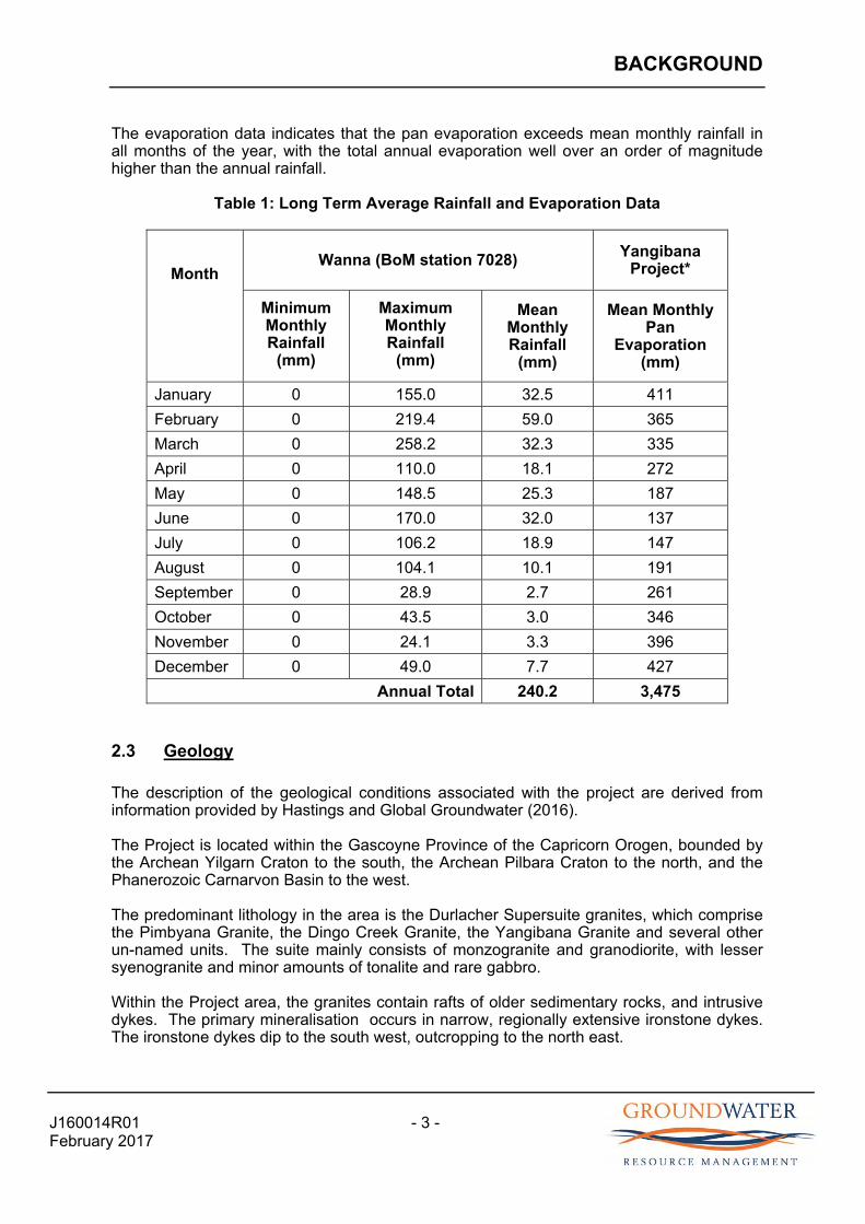
The nearest registered Bureau of Meteorological (BoM) weather station is Wanna (station number 7028), located approximately 12 km south of the Project. The station has a 98% complete data set for the 63 year period between 1 Jan 1946 to 31 October 2009. Minimum, maximum and mean monthly rainfall data is provided in Table 1. The data from Wanna indicates that the average annual rainfall is around 240 mm, with the highest rainfall occurring from January to March, closely followed by May and June.
Evaporation data is recorded at Paraburdoo (station number 7178), located 160 km north east of the Project, and Learmonth Airport (station number 5007), 290 km north west of the Project. The data from Paraburdoo and Learmonth has been scaled, based upon distance, to develop an estimate of average monthly evaporation for Yangibana, as provided in Table 1.
BACKGROUND
J160014R01 - 3 - February 2017
The evaporation data indicates that the pan evaporation exceeds mean monthly rainfall in all months of the year, with the total annual evaporation well over an order of magnitude higher than the annual rainfall.
Table 1: Long Term Average Rainfall and Evaporation Data
Month Wanna (BoM station 7028) Yangibana
Project*
Minimum Monthly Rainfall
(mm)
Maximum Monthly Rainfall
(mm)
Mean Monthly Rainfall
(mm)
Mean Monthly Pan
Evaporation (mm)
January 0 155.0 32.5 411
February 0 219.4 59.0 365
March 0 258.2 32.3 335
April 0 110.0 18.1 272
May 0 148.5 25.3 187
June 0 170.0 32.0 137
July 0 106.2 18.9 147
August 0 104.1 10.1 191
September 0 28.9 2.7 261
October 0 43.5 3.0 346
November 0 24.1 3.3 396
December 0 49.0 7.7 427
Annual Total 240.2 3,475
2.3 Geology
The description of the geological conditions associated with the project are derived from information provided by Hastings and Global Groundwater (2016).
The Project is located within the Gascoyne Province of the Capricorn Orogen, bounded by the Archean Yilgarn Craton to the south, the Archean Pilbara Craton to the north, and the Phanerozoic Carnarvon Basin to the west.
The predominant lithology in the area is the Durlacher Supersuite granites, which comprise the Pimbyana Granite, the Dingo Creek Granite, the Yangibana Granite and several other un-named units. The suite mainly consists of monzogranite and granodiorite, with lesser syenogranite and minor amounts of tonalite and rare gabbro.
Within the Project area, the granites contain rafts of older sedimentary rocks, and intrusive dykes. The primary mineralisation occurs in narrow, regionally extensive ironstone dykes. The ironstone dykes dip to the south west, outcropping to the north east.
BACKGROUND
J160014R01 - 4 - February 2017
The dykes carry anomalous rare earths within the monazite mineralisation. The dykes are understood to be a younger intrusive phase which has cross cut slightly older feroocarbonatite dykes, possibly leaching and upgrading rare earths (and base metals) from them. The carbonatite dykes (which form the Gifford Creek Carbonatite Complex), along with associated fenitic alteration, is considered to be sourced from (an as yet undiscovered) carbonatite intrusion at depth, which could potentially host significant rare earths and base metals.
2.4 Regional Hydrogeology
The description of the regional hydrogeological conditions are derived from publicly available information provided by Hastings, and the desktop study completed by Global Groundwater (2016).
The project is located within the Bangemall/Capricorn Groundwater subarea of the Gascoyne Groundwater area. Groundwater resources within the subarea comprise alluvium, calcrete, palaeochannel and fractured rock aquifers.
The hydrogeology of the area is characterised by a south westerly draining system, coincident with the Lyons River surface water catchment. Alluvial cover is typically thin or absent across the majority of the area, but thickens near the creeks and major drainages.
Groundwater occurrences in the area predominantly occur as fractured bedrock aquifers, whereby permeability in the natural rock is enhanced by fracturing, dissolution and chemical weathering. Away from the fractures permeability in the bedrock is typically low. In the Project are the extensive ironstone dykes form a potentially significant fractured rock aquifer. The ironstone aquifer is discussed in more detail later in this report.
Groundwater occurrences are also known to occur in calcrete aquifers in the area. Thorpe (1990) identified that calcrete extends to depths of 30 m within the Edmund and Lyons Rivers, and likely extends over large areas beneath the alluvial cover.
Small amounts of groundwater can occur in alluvium associated with the larger drainage systems. However away from the larger drainage systems the alluvium is typically absent or of insufficient thickness to extend below the water table.
Groundwater is recharged by direct rainfall infiltration or by stream flow during episodic rainfall events. Recharge is expected to be highest following streamflow events, in locations where the alluvium overlies more permeable units (such as calcrete or fractured basement). Groundwater recharge by direct infiltration of rainfall is likely to be minor.
Groundwater quality in the area is typically fresh to brackish, with salinities ranging from about 900 to 4,000 mg/L Total Dissolved Solids (TDS). The lowest salinity groundwater occurs closest to the areas of recharge, with salinity increasing away from the recharge areas.
BACKGROUND
J160014R01 - 5 - February 2017
2.5 Other Groundwater Users
A search of bore records within a 20 km radius of Bald Hills was carried using the Water Information Reporting (WIR) database, which is managed by the Department of Water (DoW).
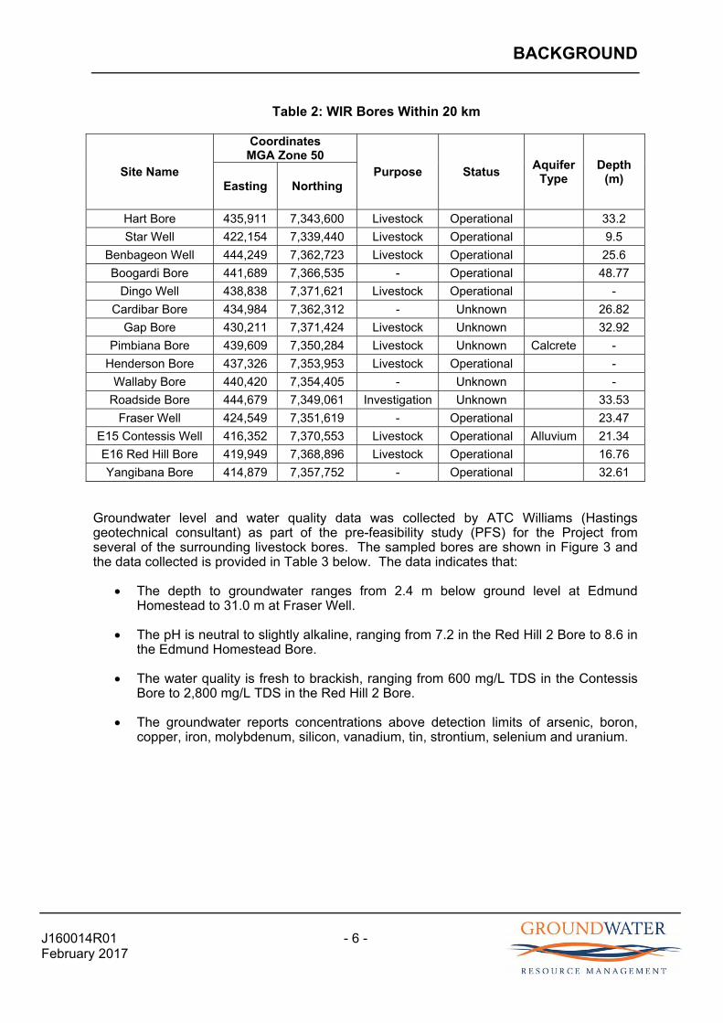
The WIR data indicates that there are 15 registered bores within 20 km of the project tenements. A summary of the bore information is provided in Table 2 below, and the bore locations closest to the Project area are shown in Figure 3.
The WIR data indicates that:
The closest bores to the proposed pits are Yangibana Bore and Fraser Well, located 5 km south of Yangibana and 5 km west of Fraser’s deposits, respectively. The bores are listed as being of unknown type and status. However it is believed the bores are operational livestock bores.
Nine of the 15 bores are listed as livestock bores. The Roadside bore is listed as an investigation bore, and the remaining five bores are of unknown type. However it is presumed that the bores listed as unknown type are also livestock bores, given the land use in the area.
Pimbiana Bore is registered as being installed into a calcrete aquifer, and is located approximately 10 km east of Fraser’s. Pimbiana Bore is not near the Lyons or Edmund Rivers (as shown in Figure 3) and occurrence of calcrete in this location suggests calcrete may not be restricted to the major rivers, and may extend over larger distances beneath the alluvial cover, as suggested by Thorpe (1990).
Contessis Well is listed as installed into an alluvial aquifer, and is located approximately 9 km north of Yangibana.
The remainder of the listed bores are of unknown aquifer type. However, based upon the shallow drilled depths and the locations, it is likely the bores are installed into either alluvial, calcrete or shallow bedrock aquifers.
BACKGROUND
J160014R01 - 6 - February 2017
Table 2: WIR Bores Within 20 km
Site Name
Coordinates MGA Zone 50
Purpose Status Aquifer
Type Depth
(m) Easting Northing
Hart Bore 435,911 7,343,600 Livestock Operational 33.2
Star Well 422,154 7,339,440 Livestock Operational 9.5
Benbageon Well 444,249 7,362,723 Livestock Operational 25.6
Boogardi Bore 441,689 7,366,535 - Operational 48.77
Dingo Well 438,838 7,371,621 Livestock Operational -
Cardibar Bore 434,984 7,362,312 - Unknown 26.82
Gap Bore 430,211 7,371,424 Livestock Unknown 32.92
Pimbiana Bore 439,609 7,350,284 Livestock Unknown Calcrete -
Henderson Bore 437,326 7,353,953 Livestock Operational -
Wallaby Bore 440,420 7,354,405 - Unknown -
Roadside Bore 444,679 7,349,061 Investigation Unknown 33.53
Fraser Well 424,549 7,351,619 - Operational 23.47
E15 Contessis Well 416,352 7,370,553 Livestock Operational Alluvium 21.34
E16 Red Hill Bore 419,949 7,368,896 Livestock Operational 16.76
Yangibana Bore 414,879 7,357,752 - Operational 32.61
Groundwater level and water quality data was collected by ATC Williams (Hastings geotechnical consultant) as part of the pre-feasibility study (PFS) for the Project from several of the surrounding livestock bores. The sampled bores are shown in Figure 3 and the data collected is provided in Table 3 below. The data indicates that:
The depth to groundwater ranges from 2.4 m below ground level at Edmund Homestead to 31.0 m at Fraser Well.
The pH is neutral to slightly alkaline, ranging from 7.2 in the Red Hill 2 Bore to 8.6 in the Edmund Homestead Bore.
The water quality is fresh to brackish, ranging from 600 mg/L TDS in the Contessis Bore to 2,800 mg/L TDS in the Red Hill 2 Bore.
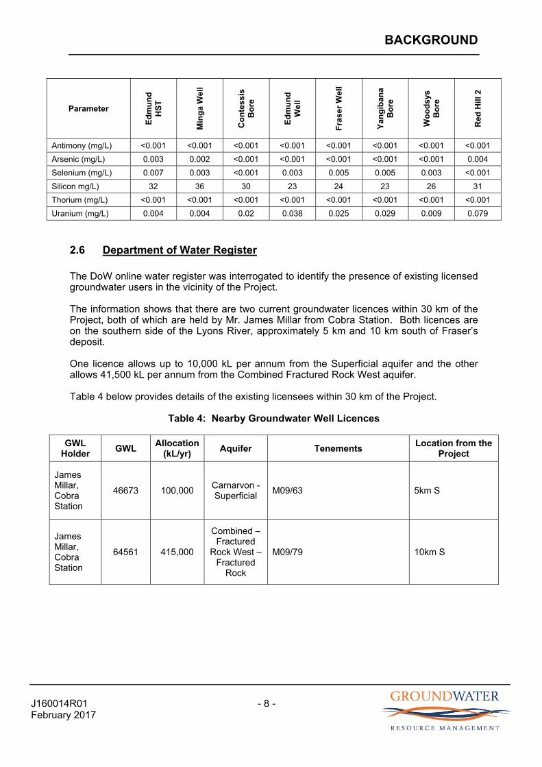
The groundwater reports concentrations above detection limits of arsenic, boron, copper, iron, molybdenum, silicon, vanadium, tin, strontium, selenium and uranium.

BACKGROUND
J160014R01 - 7 - February 2017
Table 3: Livestock Bore Data
Parameter
Ed
mu
nd
H
ST
Min
ga
Wel
l
Co
nte
ssis
B
ore
Ed
mu
nd
W
ell
Fra
ser
Wel
l
Yan
gib
ana
Bo
re
Wo
od
sys
Bo
re
Red
Hill
2
Easting (MGA z50) 410,186 407,894 416,349 405,351 424,854 414,866 413,896 419,832
Northing(MGA z50) 7,371,981 7,368,128 7,370,735 7,354,106 7,351,570 7,357,878 7,346,769 7,368,605
SWL (June 2015) 2.40 2.60 14.90 9.10 31.90 10.6 7.30 9.20
pH 8.6 8.2 8.5 7.9 8.0 7.5 7.7 7.2
TDS (mg/L) 1,400 920 600 2,200 1,600 1,600 1,800 2,800
TSS (mg/L) <5 <5 7 17 <5 <5 <5 76
Alkalinity (mgCaCO3/L)
300 520 360 430 410 360 440 440
Acidity(mgCaCO3/L) 82 120 77 130 93 120 140 200
Phosphorus (mg/L) 0.09 0.12 0.06 0.07 0.14 0.04 0.12 0.39
Sulphate (mg/L) 330 110 45 320 160 180 250 830
Chloride (mg/L) 270 110 95 810 570 530 590 710
Fluoride (mg/L) 1.4 2.3 2.5 2.9 3 2.2 1.3 4
Nitrate (mg/L) 8.97 6.5 0.05 17 12 18 12.98 -
Hardness (mgCaCO3/L)
535 336 273 609 282 608 728 1,160
Aluminium (mg/L) <0.1 <0.1 <0.1 0.2 <0.1 <0.1 <0.1 0.9
Total Iron (mg/L) 0.15 0.07 0.03 0.22 0.02 0.02 <0.01 1.5
Sulphur (mg/L) 96 38 17 110 52 60 79 250
Calcium (mg/L) 66 39 30 79 47 120 110 250
Magnesium (mg/L) 90 58 48 100 40 75 110 130
Sodium (mg/L) 280 150 70 610 550 350 380 620
Beryllium (mg/L) <0.1 <0.1 <0.1 <0.1 <0.1 <0.1 <0.1 <0.1
Boron (mg/L) 1 0.5 0.26 1.4 0.83 0.55 0.8 2.1
Chromium (mg/L <0.01 <0.01 <0.01 <0.01 <0.01 <0.01 <0.01 <0.01
Cadmium (mg/L) <0.002 <0.002 <0.002 <0.002 <0.002 <0.002 <0.002 <0.002
Cobalt (mg/L) <0.01 <0.01 <0.01 <0.01 <0.01 <0.01 <0.01 <0.01
Copper (mg/L) <0.01 <0.01 0.02 0.04 <0.01 <0.01 <0.01 <0.01
Iron (mg/L) 0.07 <0.01 <0.01 <0.01 <0.01 <0.01 <0.01 0.19
Lead (mg/L) <0.01 <0.01 <0.01 <0.01 <0.01 <0.01 <0.01 <0.01
Manganese (mg/L) <0.01 <0.01 <0.01 <0.01 <0.01 <0.01 <0.01 0.87
Molybdenum(mg/L) <0.01 0.01 0.01 0.01 0.02 <0.01 <0.01 0.01
Nickel (mg/L) <0.01 <0.01 <0.01 <0.01 <0.01 <0.01 <0.01 <0.01
Silver (mg/L) <0.01 <0.01 <0.01 <0.01 <0.01 <0.01 <0.01 <0.01
Strontium (mg/L) 0.76 0.41 0.3 1.1 0.52 0.92 0.82 2.2
Tin (mg/L) <0.01 <0.01 0.02 <0.01 <0.01 <0.01 <0.01 <0.01
Titanium (mg/L) <0.01 <0.01 <0.01 <0.01 <0.01 <0.01 <0.01 <0.01
Vanadium (mg/L) 0.04 0.05 <0.01 0.03 <0.01 <0.01 0.01 <0.01
Zinc (mg/L) <0.01 <0.01 <0.01 <0.01 <0.01 <0.01 <0.01 <0.01
BACKGROUND
J160014R01 - 8 - February 2017
Parameter
Ed
mu
nd
H
ST
Min
ga
Wel
l
Co
nte
ssis
B
ore
Ed
mu
nd
W
ell
Fra
ser
Wel
l
Yan
gib
ana
Bo
re
Wo
od
sys
Bo
re
Red
Hill
2
Antimony (mg/L) <0.001 <0.001 <0.001 <0.001 <0.001 <0.001 <0.001 <0.001
Arsenic (mg/L) 0.003 0.002 <0.001 <0.001 <0.001 <0.001 <0.001 0.004
Selenium (mg/L) 0.007 0.003 <0.001 0.003 0.005 0.005 0.003 <0.001
Silicon mg/L) 32 36 30 23 24 23 26 31
Thorium (mg/L) <0.001 <0.001 <0.001 <0.001 <0.001 <0.001 <0.001 <0.001
Uranium (mg/L) 0.004 0.004 0.02 0.038 0.025 0.029 0.009 0.079
2.6 Department of Water Register
The DoW online water register was interrogated to identify the presence of existing licensed groundwater users in the vicinity of the Project.
The information shows that there are two current groundwater licences within 30 km of the Project, both of which are held by Mr. James Millar from Cobra Station. Both licences are on the southern side of the Lyons River, approximately 5 km and 10 km south of Fraser’s deposit.
One licence allows up to 10,000 kL per annum from the Superficial aquifer and the other allows 41,500 kL per annum from the Combined Fractured Rock West aquifer.
Table 4 below provides details of the existing licensees within 30 km of the Project.
Table 4: Nearby Groundwater Well Licences
GWL Holder
GWL Allocation
(kL/yr) Aquifer Tenements
Location from the Project
James Millar, Cobra Station
46673 100,000 Carnarvon - Superficial
M09/63 5km S
James Millar, Cobra Station
64561 415,000
Combined – Fractured
Rock West – Fractured
Rock
M09/79 10km S

BACKGROUND
J160014R01 - 9 - February 2017
2.7 Groundwater Dependent Ecosystems
A review of the Bureau of Meteorology’s (BoM’s) GDE Atlas indicates that the Project area is classified as having:
No to low potential for groundwater interaction with vegetation reliant on subsurface groundwater.
No identified vegetation GDE’s reliant of surface expression of groundwater (rivers, springs, wetlands).
No identified subterranean GDEs (caves or aquifers).
The nearest significant GDE is along the Lyons River (to the south of the Project) and the Edmund River (to the west of the Project), which both report vegetation GDE’s reliant on surface water and groundwater.
A copy of the GDE Atlas report, for an area of 25 km from 428,000 mE and 7,356,000 mN (Bald Hills) is provided as Appendix A.
Ecoscape (Australia) Pty Ltd (2015)1 completed a flora and vegetation assessment of the broad Project region, including the proposed development envelope. The assessment reported the presence of one vegetation type which represents a GDE (presence of Eucalyptus camaldulensis), and three other vegetation types represent potential GDEs (presence of Eucalyptus victrix). General GDE vegetation types are located outside the proposed disturbance footprint, except where linear infrastructure crosses the Lyons River, Fraser Creek and Yangibana Creek.
Hastings has initiated subterranean fauna studies in the Project area, as part of the DFS process, and the outcomes will be discussed further in the Stage II study report.
1 Ecoscape (Australia) Pty Ltd (2015) “Yangibana Project Biological Assessment: Flora and Vegetation” unpublished report prepared for Hastings Technology Metals Limited, December 2015
SELECTION OF TESTING LOCATIONS
J160014R01 - 10 - February 2017
3.0 SELECTION OF TESTING LOCATIONS
A review was carried out by GRM of the available hydrogeological and geological data collected for the deposits to gain an understanding of likely hydrogeological conditions and confirm suitable testing locations.
The information used for the review included the geological drill-hole database, records of groundwater intersects in resource drill-holes, preliminary testing locations proposed by ATC Williams (geotechnical consultants), and information provided by Hastings geologists.
The available information was qualitative but indicated consistent groundwater inflows associated with the ironstone dykes, and generally low permeability conditions in the footwall and hanging wall granite.
The results of the review were used to revise the preliminary testing locations provided by ATC Williams, to develop a Stage I field testing programme.
The Stage I programme was aimed at providing sufficient data for 3D groundwater flow modelling, and consequently included small scale hydraulic testing and 48 hour test pumping, to provide an indication of hydraulic parameters for input to the groundwater flow model.
The details of the field investigations are discussed in Section 4.0.
STAGE I FIELD INVESTIGATIONS
J160014R01 - 11 - February 2017
4.0 STAGE 1 FIELD INVESTIGATIONS
Field investigations to assess the likely dewatering rates for the three proposed pits comprised the following:
Groundwater exploration drilling to collect hydrogeological data, and identify potential test bore locations (Fraser’s and Bald Hills). Note no exploration drilling was required at Yangibana as an existing drilling supply bore was available for testing purposes.
Airlift recovery testing of groundwater exploration holes and/or from selected existing mineral exploration drill-holes to provide a range of estimates of hydraulic conductivity within the mining area.
Install test bores at Fraser’s and Bald Hills, and undertake test pumping (all pits) to estimate hydraulic parameters for the fractured rock aquifer and identify any potential boundary conditions.
Collection of groundwater samples for laboratory analysis from the deposits.
4.1 Exploration Drilling
Hydrogeological data was collected during the drilling of 6 groundwater exploration drill-holes (two at Fraser’s and four at Bald Hill), which varied in depth from 70 to 102 m deep. The selected drill-holes targeted the ironstone dyke on the down-dip side of the pit, for the purpose of collecting hydrogeological information as well as locating suitable test bore locations.
The drilling was undertaken by Three Rivers Drilling between 20 October and 13 November 2016, using reverse circulation (RC) methods. The programme was overseen by GRM and Hastings field personnel who were responsible for the collection and field assessment of geological and hydrogeological data.
The exploration holes were drilled under a granted Licence to Construct or Alter a Well CAW183123(1), issued by the DoW on 3 August 2016. The CAW is provided in Appendix B.
A summary of the drilling results is provided in Table 5 and the bore logs are provided in Appendix C.
The exploration drilling results indicate the following:
Groundwater inflows were associated with the ironstone dykes.
Away from the ironstone dykes, the granite reported low groundwater inflows.
There were no reported inflows associated with alluvium or calcrete.
The two most prospective drill-holes (FRW01 at Fraser’s and BHW04 at Bald Hill) reported modest groundwater inflows, with airlift yields of between 1.5 and 2.2 L/sec.
The exploration drilling results support the presence of a discrete fractured rock aquifer associated with the ironstone dykes.

STAGE I FIELD INVESTIGATIONS
J160014R01 - 12 - February 2017
It should be noted that RC drilling generally under-predicts yields, due to the narrow annulus between the drill rod and the drill-hole. Higher yields were reported during airlift recovery testing, as discussed in Section 4.2
Table 5: Exploration Drilling Results
Location Hole mE MGA
Zn50 mN MGA
Zn50 RL
(mAHD)Depth (m)
Max Airlift Yield During
Drilling (L/sec)
Fraser’s FRW1 429,941 7,351,211 350.5 110 1.5
FRW2 429,804 7,351,086 343.0 96 1.2
Bald Hill
BHW1 427,958 7,356,494 355.7 70 <1
BHW2 428,017 7,356,253 353.6 85 <1
BHW3 428,064 7,356,105 350.5 100 <1
BHW4 428,189 7,356,019 346.7 102 2.9
4.2 Hydraulic Testing
Airlift recovery testing of 12 drill-holes, comprising 3 locations at Fraser’s, seven locations at Bald Hill and two locations at Yangibana, was conducted between October and December 2016. The locations comprised both existing resource drill-holes and the water exploration drill-holes completed as part of this programme.
The testing was undertaken by a combination of GRM and Hastings personnel, using the services of Three Rivers Drilling.
The testing methodology comprised:
i. A water level measurement was collected prior to testing.
ii. Galvanised pipe (50 mm diameter) was run down the existing drill-hole to about 12 m above the base of the hole.
iii. The drill-hole was airlifted until the flow stabilised (around an hour).
iv. During airlifting yield measurements (using a V Notch weir) and water quality parameters were recorded at regular intervals.
v. At the completion of airlifting the galvanized pipe was un-coupled and groundwater recovery measurements collected through the inner tube using a combination of pressure transducers and manual measurements, until the recovery came to within 90% of the standing water level.
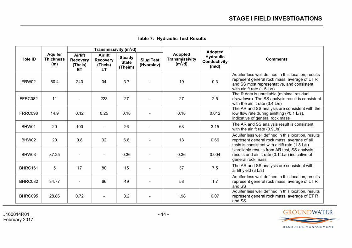
The test data was analysed using a combination of standard analytical methods including Theis (1935) and the Theim steady state method. The resulting transmissivities from the various testing methods were then reviewed and an adopted hydraulic conductivity value was assigned for each test location.
It should be noted, the recovery data for drill-hole BHRC097 was erroneous and consequently a slug test was conducted for this drill-hole. The slug test data was analysed using Hvorslev (1951).
STAGE I FIELD INVESTIGATIONS
J160014R01 - 13 - February 2017
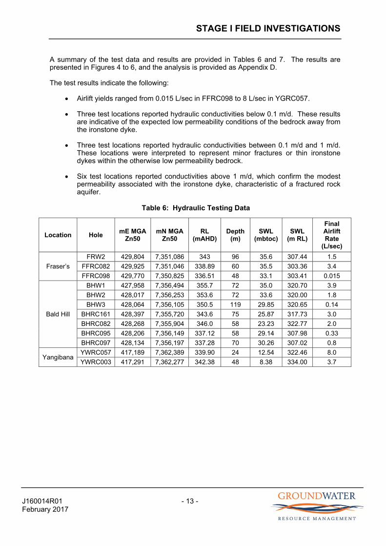
A summary of the test data and results are provided in Tables 6 and 7. The results are presented in Figures 4 to 6, and the analysis is provided as Appendix D.
The test results indicate the following:
Airlift yields ranged from 0.015 L/sec in FFRC098 to 8 L/sec in YGRC057.
Three test locations reported hydraulic conductivities below 0.1 m/d. These results are indicative of the expected low permeability conditions of the bedrock away from the ironstone dyke.
Three test locations reported hydraulic conductivities between 0.1 m/d and 1 m/d. These locations were interpreted to represent minor fractures or thin ironstone dykes within the otherwise low permeability bedrock.
Six test locations reported conductivities above 1 m/d, which confirm the modest permeability associated with the ironstone dyke, characteristic of a fractured rock aquifer.
Table 6: Hydraulic Testing Data
Location Hole mE MGA
Zn50 mN MGA
Zn50 RL
(mAHD) Depth
(m) SWL
(mbtoc) SWL
(m RL)
Final Airlift Rate
(L/sec)
Fraser’s
FRW2 429,804 7,351,086 343 96 35.6 307.44 1.5
FFRC082 429,925 7,351,046 338.89 60 35.5 303.36 3.4
FFRC098 429,770 7,350,825 336.51 48 33.1 303.41 0.015
Bald Hill
BHW1 427,958 7,356,494 355.7 72 35.0 320.70 3.9
BHW2 428,017 7,356,253 353.6 72 33.6 320.00 1.8
BHW3 428,064 7,356,105 350.5 119 29.85 320.65 0.14
BHRC161 428,397 7,355,720 343.6 75 25.87 317.73 3.0
BHRC082 428,268 7,355,904 346.0 58 23.23 322.77 2.0
BHRC095 428,206 7,356,149 337.12 58 29.14 307.98 0.33
BHRC097 428,134 7,356,197 337.28 70 30.26 307.02 0.8
Yangibana YWRC057 417,189 7,362,389 339.90 24 12.54 322.46 8.0
YWRC003 417,291 7,362,277 342.38 48 8.38 334.00 3.7
STAGE I FIELD INVESTIGATIONS
J160014R01 - 14 - February 2017
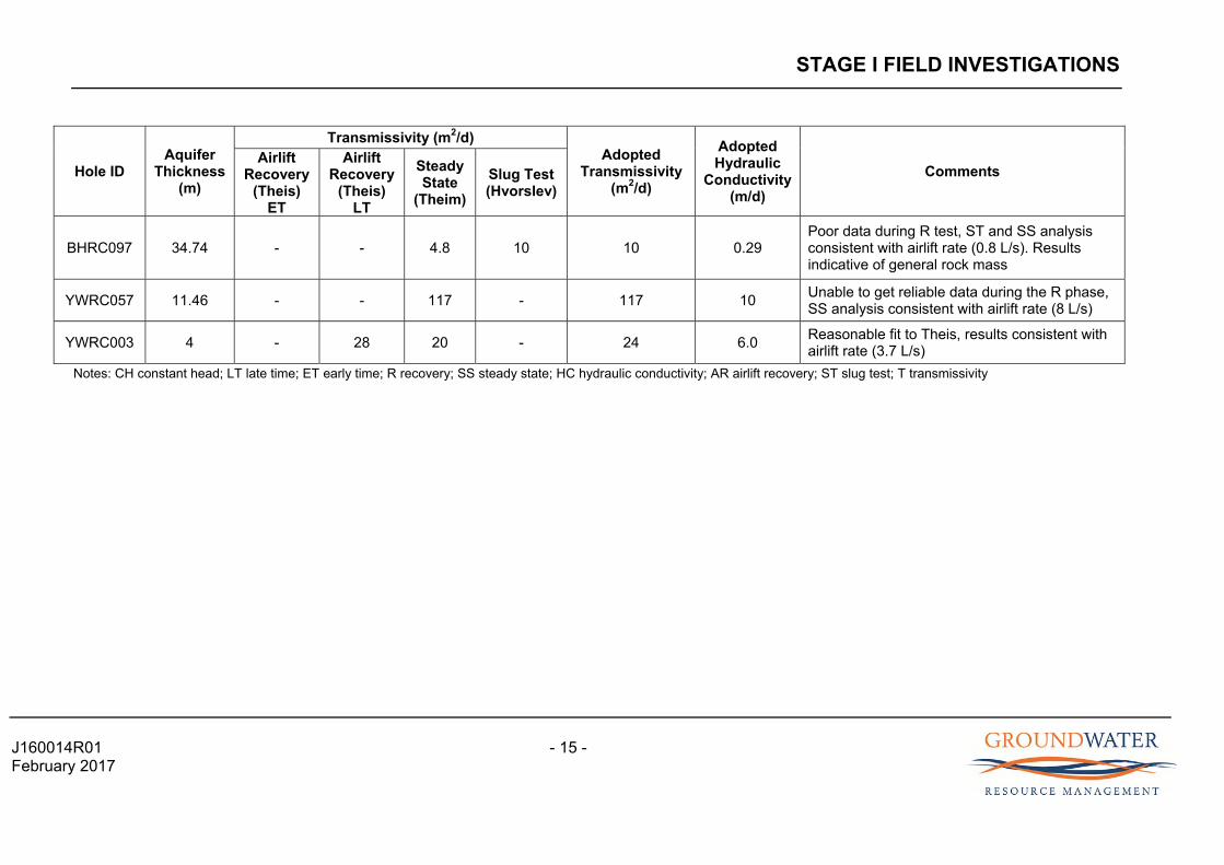
Table 7: Hydraulic Test Results
Hole ID Aquifer
Thickness (m)
Transmissivity (m2/d) Adopted
Transmissivity (m2/d)
Adopted Hydraulic
Conductivity (m/d)
Comments Airlift
Recovery (Theis)
ET
Airlift Recovery
(Theis) LT
Steady State
(Theim)
Slug Test (Hvorslev)
FRW02 60.4 243 34 3.7 - 19 0.3
Aquifer less well defined in this location, results represent general rock mass, average of LT R and SS most representative, and consistent with airlift rate (1.5 L/s)
FFRC082 11 - 223 27 - 27 2.5 The R data is unreliable (minimal residual drawdown). The SS analysis result is consistent with the airlift rate (3.4 L/s)
FRRC098 14.9 0.12 0.25 0.18 - 0.18 0.012 The AR and SS analysis are consistent with the low flow rate during airlifting (<0.1 L/s), indicative of general rock mass
BHW01 20 100 - 26 - 63 3.15 The AR and SS analysis result is consistent with the airlift rate (3.9L/s)
BHW02 20 0.8 32 6.8 - 13 0.66 Aquifer less well defined in this location, results represent general rock mass, average of all tests is consistent with airlift rate (1.8 L/s)
BHW03 87.25 - - 0.36 - 0.36 0.004 Unreliable results from AR test, SS analysis results and airlift rate (0.14L/s) indicative of general rock mass
BHRC161 5 17 80 15 - 37 7.5 The AR and SS analysis are consistent with airlift yield (3 L/s)
BHRC082 34.77 - 66 49 - 58 1.7 Aquifer less well defined in this location, results represent general rock mass, average of LT R and SS
BHRC095 28.86 0.72 - 3.2 - 1.98 0.07 Aquifer less well defined in this location, results represent general rock mass, average of ET R and SS
STAGE I FIELD INVESTIGATIONS
J160014R01 - 15 - February 2017
Hole ID Aquifer
Thickness (m)
Transmissivity (m2/d) Adopted
Transmissivity (m2/d)
Adopted Hydraulic
Conductivity (m/d)
Comments Airlift
Recovery (Theis)
ET
Airlift Recovery
(Theis) LT
Steady State
(Theim)
Slug Test (Hvorslev)
BHRC097 34.74 - - 4.8 10 10 0.29 Poor data during R test, ST and SS analysis consistent with airlift rate (0.8 L/s). Results indicative of general rock mass
YWRC057 11.46 - - 117 - 117 10 Unable to get reliable data during the R phase, SS analysis consistent with airlift rate (8 L/s)
YWRC003 4 - 28 20 - 24 6.0 Reasonable fit to Theis, results consistent with airlift rate (3.7 L/s)
Notes: CH constant head; LT late time; ET early time; R recovery; SS steady state; HC hydraulic conductivity; AR airlift recovery; ST slug test; T transmissivity
STAGE I FIELD INVESTIGATIONS
J160014R01 - 16 - February 2017
4.3 Test Bore Installation
Two test production bores, FRW03 and BHW05, were installed adjacent to the two highest yielding exploration drill-holes (FRW01 and BHW04). Please note that FRW03 was referred to as FRW01 during the field investigations, but has subsequently been re-named to maintain consistent nomenclature and differentiate it from the original FRW01 drill-hole.
Drill-holes FRW01 and BHW04 were constructed as temporary monitoring bores for the purposes of test pumping, with the installation of 50 mm uPVC casing.
The test production bores were drilled and constructed by Three Rivers Drilling and overseen by GRM and Hastings personnel. The bores were installed under a granted Licence to Construct or Alter a Well CAW183123(1), issued by the DoW on 3 August 2016. The CAW is provided as Appendix B.
The production bore installation methodology comprised:
Collaring to 3 m, using 15.5 inch diameter air rotary methods.
Installation of 10 inch diameter steel surface casing to 2 to 3 m depth, cement grouted.
Drilling a pilot hole and then reaming out to 10 inch diameter hole to depth using air rotary methods.
Installation of 155 mm class 9 uPVC casing, slotted over the aquifer sequence, as identified from drill-cuttings and from geological logs from the original exploration hole, and capped at its base using an external uPVC end-cap.
Installation of +3.2 to 6.4 mm graded gravel pack in the annulus from the base of the bore to just below surface.
Placement of an annular bentonite seal from the top of the gravel packed interval to surface to prevent surface water ingress.
Airlift development of the bore for a period of at least 2 hours, to remove fine sediment from within the gravel pack and adjacent formation.
Completion of the bore with a concrete plinth, and uPVC end-cap.
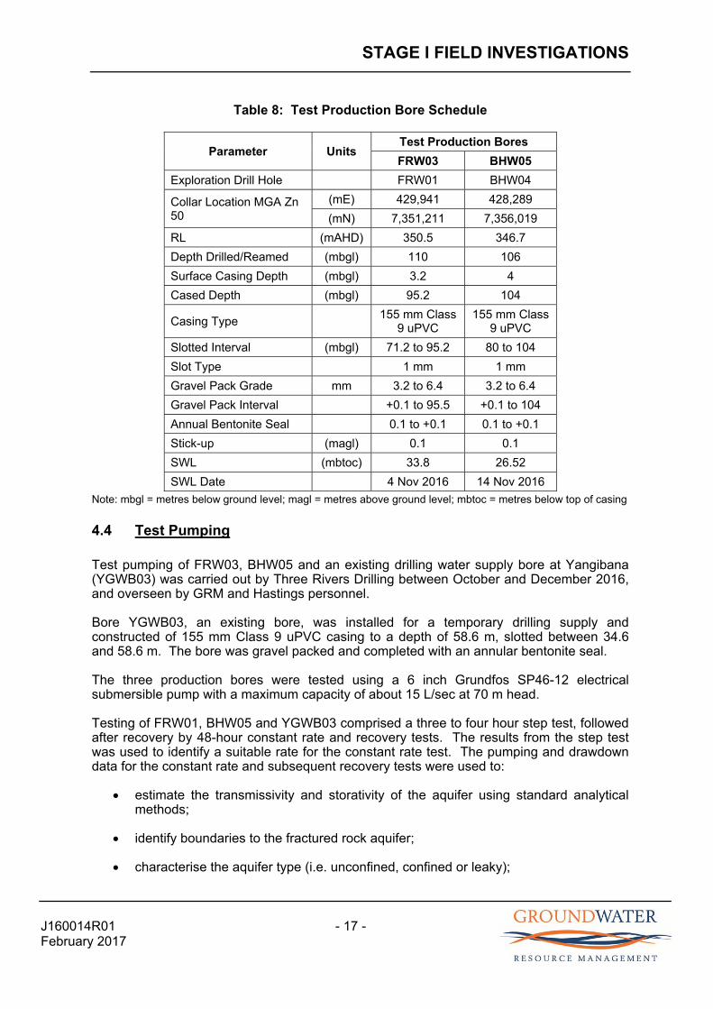
The details of the installed test bores are provided in Table 8, and bore logs are provided in Appendix C.
STAGE I FIELD INVESTIGATIONS
J160014R01 - 17 - February 2017
Table 8: Test Production Bore Schedule
Parameter Units Test Production Bores
FRW03 BHW05
Exploration Drill Hole FRW01 BHW04
Collar Location MGA Zn 50
(mE) 429,941 428,289
(mN) 7,351,211 7,356,019
RL (mAHD) 350.5 346.7
Depth Drilled/Reamed (mbgl) 110 106
Surface Casing Depth (mbgl) 3.2 4
Cased Depth (mbgl) 95.2 104
Casing Type
155 mm Class 9 uPVC
155 mm Class 9 uPVC
Slotted Interval (mbgl) 71.2 to 95.2 80 to 104
Slot Type 1 mm 1 mm
Gravel Pack Grade mm 3.2 to 6.4 3.2 to 6.4
Gravel Pack Interval +0.1 to 95.5 +0.1 to 104
Annual Bentonite Seal 0.1 to +0.1 0.1 to +0.1
Stick-up (magl) 0.1 0.1
SWL (mbtoc) 33.8 26.52
SWL Date 4 Nov 2016 14 Nov 2016
Note: mbgl = metres below ground level; magl = metres above ground level; mbtoc = metres below top of casing
4.4 Test Pumping
Test pumping of FRW03, BHW05 and an existing drilling water supply bore at Yangibana (YGWB03) was carried out by Three Rivers Drilling between October and December 2016, and overseen by GRM and Hastings personnel.
Bore YGWB03, an existing bore, was installed for a temporary drilling supply and constructed of 155 mm Class 9 uPVC casing to a depth of 58.6 m, slotted between 34.6 and 58.6 m. The bore was gravel packed and completed with an annular bentonite seal.
The three production bores were tested using a 6 inch Grundfos SP46-12 electrical submersible pump with a maximum capacity of about 15 L/sec at 70 m head.
Testing of FRW01, BHW05 and YGWB03 comprised a three to four hour step test, followed after recovery by 48-hour constant rate and recovery tests. The results from the step test was used to identify a suitable rate for the constant rate test. The pumping and drawdown data for the constant rate and subsequent recovery tests were used to:
estimate the transmissivity and storativity of the aquifer using standard analytical methods;
identify boundaries to the fractured rock aquifer;
characterise the aquifer type (i.e. unconfined, confined or leaky);
STAGE I FIELD INVESTIGATIONS
J160014R01 - 18 - February 2017
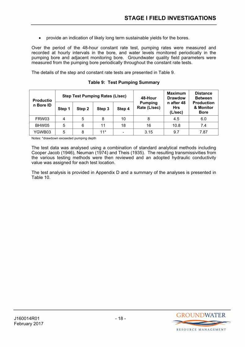
provide an indication of likely long term sustainable yields for the bores.
Over the period of the 48-hour constant rate test, pumping rates were measured and recorded at hourly intervals in the bore, and water levels monitored periodically in the pumping bore and adjacent monitoring bore. Groundwater quality field parameters were measured from the pumping bore periodically throughout the constant rate tests.
The details of the step and constant rate tests are presented in Table 9.
Table 9: Test Pumping Summary
Production Bore ID
Step Test Pumping Rates (L/sec) 48-Hour Pumping
Rate (L/sec)
Maximum Drawdown after 48
Hrs (L/sec)
Distance Between
Production & Monitor
Bore Step 1 Step 2 Step 3 Step 4
FRW03 4 5 8 10 8 4.5 6.0
BHW05 5 6 11 18 16 10.8 7.4
YGWB03 5 8 11* - 3.15 9.7 7.87
Notes: *drawdown exceeded pumping depth
The test data was analysed using a combination of standard analytical methods including Cooper Jacob (1946), Neuman (1974) and Theis (1935). The resulting transmissivities from the various testing methods were then reviewed and an adopted hydraulic conductivity value was assigned for each test location.
The test analysis is provided in Appendix D and a summary of the analyses is presented in Table 10.

STAGE I FIELD INVESTIGATIONS
J160014R01 - 19 - February 2017
Table 10: Test Pumping Analysis Results
Hole ID Aquifer
Thickness (m)
Transmissivity (m2/d)
Adopted Transmissivity
(m2/d)
Adopted Hydraulic
Conductivity (m/d)
Storativity (S)
Comments Constant Rate ET (Cooper Jacob)
Constant Rate LT (Cooper Jacob)
Constant Rate
(Neuman)
Recovery ET
(Theis)
Recovery LT
(Theis)
FRW03 11 - 28 - 329 197 28 2.5 -
CRT indicates boundary condition at about 1000 mins, LT data for CRT most representative
FRW01 11 - 28 - - - 28 2.5 - Results consistent with pumping bore, CRT LT data most representative
BHW05 20 236 75 - 207 217 75 3.75 1.0 E-04
CRT indicated boundary condition at about 1000 mins, LT data for CRT most representative
BHW04 20 214 75 - 232 - 75 3.75 4.0 E-04 Results consistent with pumping bore
YGWB03 10 - 55 - 30 83 56 5.6 1.0 E-06 Poor curve fitting, average of all test data
YGWB03obs 10 - 36 10 23 78 37 3.7 - Good curve fit with Neuman, results consistent with pumping bore
Notes: CRT constant rate test; ET Early time; LT late time
STAGE I FIELD INVESTIGATIONS
J160014R01 - 20 - February 2017
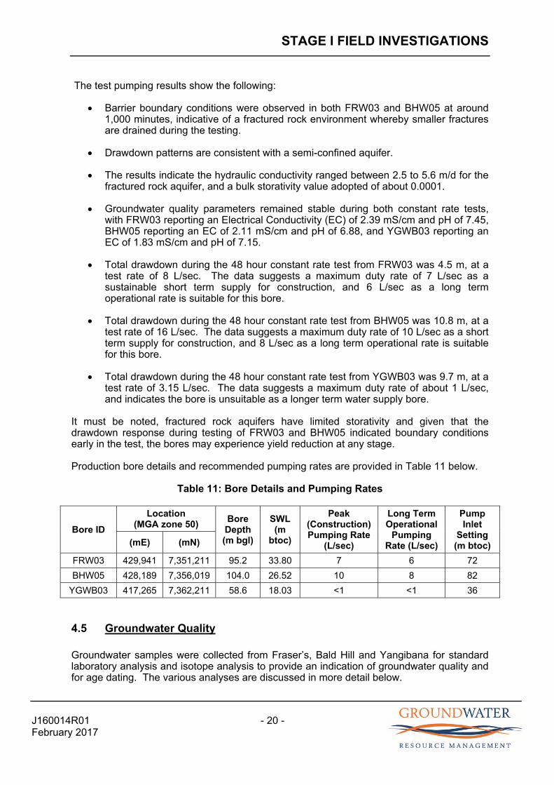
The test pumping results show the following:
Barrier boundary conditions were observed in both FRW03 and BHW05 at around 1,000 minutes, indicative of a fractured rock environment whereby smaller fractures are drained during the testing.
Drawdown patterns are consistent with a semi-confined aquifer.
The results indicate the hydraulic conductivity ranged between 2.5 to 5.6 m/d for the fractured rock aquifer, and a bulk storativity value adopted of about 0.0001.
Groundwater quality parameters remained stable during both constant rate tests, with FRW03 reporting an Electrical Conductivity (EC) of 2.39 mS/cm and pH of 7.45, BHW05 reporting an EC of 2.11 mS/cm and pH of 6.88, and YGWB03 reporting an EC of 1.83 mS/cm and pH of 7.15.
Total drawdown during the 48 hour constant rate test from FRW03 was 4.5 m, at a test rate of 8 L/sec. The data suggests a maximum duty rate of 7 L/sec as a sustainable short term supply for construction, and 6 L/sec as a long term operational rate is suitable for this bore.
Total drawdown during the 48 hour constant rate test from BHW05 was 10.8 m, at a test rate of 16 L/sec. The data suggests a maximum duty rate of 10 L/sec as a short term supply for construction, and 8 L/sec as a long term operational rate is suitable for this bore.
Total drawdown during the 48 hour constant rate test from YGWB03 was 9.7 m, at a test rate of 3.15 L/sec. The data suggests a maximum duty rate of about 1 L/sec, and indicates the bore is unsuitable as a longer term water supply bore.
It must be noted, fractured rock aquifers have limited storativity and given that the drawdown response during testing of FRW03 and BHW05 indicated boundary conditions early in the test, the bores may experience yield reduction at any stage.
Production bore details and recommended pumping rates are provided in Table 11 below.
Table 11: Bore Details and Pumping Rates
4.5 Groundwater Quality
Groundwater samples were collected from Fraser’s, Bald Hill and Yangibana for standard laboratory analysis and isotope analysis to provide an indication of groundwater quality and for age dating. The various analyses are discussed in more detail below.
Bore ID
Location (MGA zone 50)
Bore Depth (m bgl)
SWL (m
btoc)
Peak (Construction) Pumping Rate
(L/sec)
Long Term Operational
Pumping Rate (L/sec)
Pump Inlet
Setting (m btoc) (mE) (mN)
FRW03 429,941 7,351,211 95.2 33.80 7 6 72
BHW05 428,189 7,356,019 104.0 26.52 10 8 82
YGWB03 417,265 7,362,211 58.6 18.03 <1 <1 36
STAGE I FIELD INVESTIGATIONS
J160014R01 - 21 - February 2017
4.5.1 Laboratory Analysis
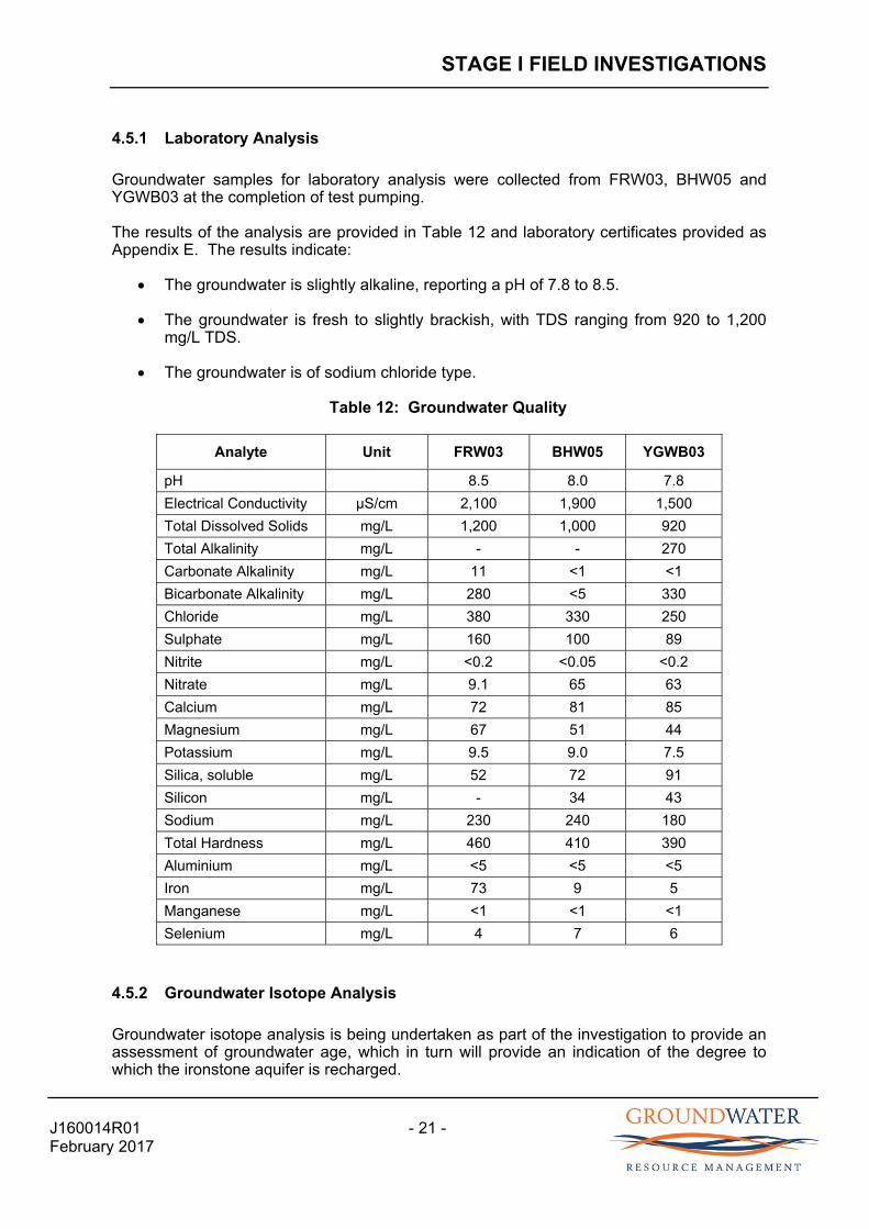
Groundwater samples for laboratory analysis were collected from FRW03, BHW05 and YGWB03 at the completion of test pumping.
The results of the analysis are provided in Table 12 and laboratory certificates provided as Appendix E. The results indicate:
The groundwater is slightly alkaline, reporting a pH of 7.8 to 8.5.
The groundwater is fresh to slightly brackish, with TDS ranging from 920 to 1,200 mg/L TDS.
The groundwater is of sodium chloride type.
Table 12: Groundwater Quality
Analyte Unit FRW03 BHW05 YGWB03
pH 8.5 8.0 7.8
Electrical Conductivity µS/cm 2,100 1,900 1,500
Total Dissolved Solids mg/L 1,200 1,000 920
Total Alkalinity mg/L - - 270
Carbonate Alkalinity mg/L 11 <1 <1
Bicarbonate Alkalinity mg/L 280 <5 330
Chloride mg/L 380 330 250
Sulphate mg/L 160 100 89
Nitrite mg/L <0.2 <0.05 <0.2
Nitrate mg/L 9.1 65 63
Calcium mg/L 72 81 85
Magnesium mg/L 67 51 44
Potassium mg/L 9.5 9.0 7.5
Silica, soluble mg/L 52 72 91
Silicon mg/L - 34 43
Sodium mg/L 230 240 180
Total Hardness mg/L 460 410 390
Aluminium mg/L <5 <5 <5
Iron mg/L 73 9 5
Manganese mg/L <1 <1 <1
Selenium mg/L 4 7 6
4.5.2 Groundwater Isotope Analysis
Groundwater isotope analysis is being undertaken as part of the investigation to provide an assessment of groundwater age, which in turn will provide an indication of the degree to which the ironstone aquifer is recharged.
STAGE I FIELD INVESTIGATIONS
J160014R01 - 22 - February 2017
GRM approached Ms. Karina Meredith1 (ANSTO Hydrogeologist) for advice regarding isotope analysis and was advised that given the construction of the bores (i.e. the ironstone aquifer is not physically isolated from the overlying granite), the groundwater in the bore will likely be a mix of different aged groundwater, and consequently age dating using radiocarbon methods will likely give misleading results.
GRM was advised that the most appropriate method of groundwater dating in this situation would be to use tritium detection dating, whereby positive detection of tritium indicates that the groundwater is less than 50 years old. Ms. Meredith suggested collecting a sample at the commencement of test pumping to assess the groundwater close to the bore (which may be a mix of groundwater from the ironstone and overlying granite) and a second sample at the end of test pumping which should represent groundwater drawn from the ironstone aquifer (given the low permeability of the granite).
A positive detection of tritium in both samples would indicate that the groundwater in the ironstone aquifer is less than 50 years old, which would suggest recent recharge.
Samples were collected during test pumping and have been submitted to the ANSTO laboratory for tritium detection. It is anticipated the results will be available by April 2017, and will be discussed in the Stage II report.
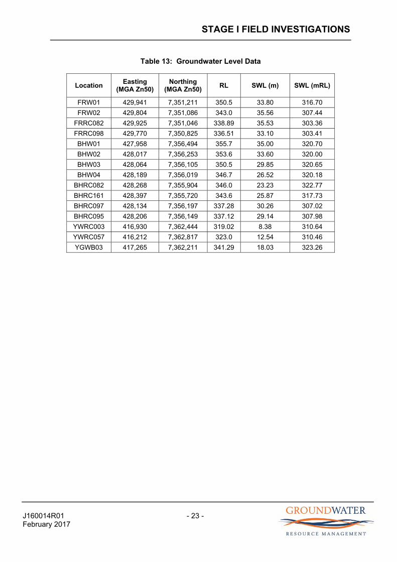
4.6 Groundwater Levels
Groundwater level measurements were collected during testing. The data is provided in Table 13, and presented in Figures 4 to 6.
The data indicates the groundwater level across the deposits range from about 309 mRL at Fraser’s, 316 mRL at Bald Hill and 323 mRL at Yangibana. The recorded groundwater levels are consistent with a regional groundwater flow direction towards the south south-west (i.e. towards the Lyons River).
1 Co-author of “Evolution of chemical and isotope composition of inorganic carbon in a complex semi-arid zone environment: Consequences for groundwater dating using radiocarbon” K.T. Meredith, L.F. Han, S.E. Hollins, D.I. Cendon, G.E. Jacobsen, A. Baker.
STAGE I FIELD INVESTIGATIONS
J160014R01 - 23 - February 2017
Table 13: Groundwater Level Data
Location Easting
(MGA Zn50) Northing
(MGA Zn50) RL SWL (m) SWL (mRL)
FRW01 429,941 7,351,211 350.5 33.80 316.70
FRW02 429,804 7,351,086 343.0 35.56 307.44
FRRC082 429,925 7,351,046 338.89 35.53 303.36
FRRC098 429,770 7,350,825 336.51 33.10 303.41
BHW01 427,958 7,356,494 355.7 35.00 320.70
BHW02 428,017 7,356,253 353.6 33.60 320.00
BHW03 428,064 7,356,105 350.5 29.85 320.65
BHW04 428,189 7,356,019 346.7 26.52 320.18
BHRC082 428,268 7,355,904 346.0 23.23 322.77
BHRC161 428,397 7,355,720 343.6 25.87 317.73
BHRC097 428,134 7,356,197 337.28 30.26 307.02
BHRC095 428,206 7,356,149 337.12 29.14 307.98
YWRC003 416,930 7,362,444 319.02 8.38 310.64
YWRC057 416,212 7,362,817 323.0 12.54 310.46
YGWB03 417,265 7,362,211 341.29 18.03 323.26
CONCEPTUAL MODEL
J160014R01 - 24 - February 2017
5.0 CONCEPTUAL MODEL
The conceptual model for the Project deposits is derived from information collected during the desktop study and the field investigations.
The conceptual model for the area recognises three hydrogeological units, which are shown schematically in Figure 7, and described below:
Hydrogeological Unit (HU) 1 comprises the alluvium and calcrete units. This unit is discontinuous within the Project area, with alluvium typically occupying low lying areas in creeks and drainage channels. Alluvium is typically absent or less than a few metres thick across the remainder of the Project area. In locations where the alluvium is sufficiently thick to extend below the water table (i.e. in the larger creeks), permeability in this unit can be modest, depending upon the composition of the alluvium, as evidenced by several stock watering bores installed into this unit. It is likely this unit could fluctuate between saturated and unsaturated seasonally, in response to streamflow. Calcrete is known to occur adjacent to the major drainages (Lyons and Edmund Rivers) and may extend over large areas beneath the alluvial cover. The calcrete is known to extend to depths of up to 30 m and permeability in this unit is likely to be modest to high. Groundwater quality within the HU1 is expected to be fresh, and there is likely to be some degree of hydraulic connection between the HU1 and HU2. The HU1 is thin to absent in the immediate area of the proposed pits, and is not shown in the schematic model provided as Figure 7.
HU2 comprises discrete ironstone units within the fresh bedrock. The ironstone units are narrow, but regionally extensive, and pinch and swell along strike as well as at depth. The ironstone thickness varies from about 1m to 20m, with an average thickness of about 4 to 5m. The ironstone outcrops to the north east, plunging to the south west, and is highly fractured and vuggy. Groundwater inflows from the HU2 are generally modest. However storage characteristics can be low, given the discrete nature of the feature. Groundwater quality in the HU2 is typically fresh to brackish, with salinity increasing away from recharge areas. Recharge to the HU2 will primarily occur where the HU2 is in contact with saturated HU1. Direct rainfall recharge (where the HU2 outcrops) and recharge from the HU3 is expected to be minimal. The HU2 is a semi-confined aquifer, somewhat confined by the overlying low permeability HU3.
HU3 comprises the intact fresh bedrock sequences (excluding the HU2 feature). The HU3 comprises granites, granodiorite and monzanites, which form the hangingwall and footwall units to the HU2. Permeability within this unit is very low, with low storage characteristics. The depth of weathering in the HU3 is quite shallow (i.e. typically less than 10 m) and whilst weathering can often enhance permeability in some regions, this has not been observed in the Project area as the weathered zone is poorly developed and typically does not extend below the water table.
The groundwater salinity in the Project area is around 1,000 mg/L TDS, with salinity typically increasing away from recharge areas.
The groundwater levels at the proposed pits are about 309 mRL at Frasers, 316 mRL at Bald Hills and 323 mRL at Yangibana, with a groundwater flow direction towards the south south― west, towards the Lyons River.

GROUNDWATER MODELLING
J160014R01 - 25 - February 2017
6.0 GROUNDWATER MODELLING
A series of three numerical groundwater flow models were constructed for the deposits and surrounding groundwater system to simulate the impacts upon the groundwater environment from mining below the water table. The models comprised:
Model 1: Fraser’s pit
Model 2: Bald Hill pit
Model 3: Yangibana pit
The models were constructed using the MODFLOW 3D finite-difference code PMWIN pre-processor.
The numerical modelling was based upon a conceptual understanding of the groundwater system (Figure 7), developed using the data collected during recent investigations. No calibration data was available. However, sensitivity analyses were run to assess the implications of varying hydraulic properties.
The numerical model setup and results are discussed below.
6.1 Model Mesh and Layers
The models was constructed using three layers, with Layer 1 (L1) representing the hanging wall HU3, L2 representing HU2, and L3 representing the footwall HU3. The geometry of the layers reflected the conceptual model (Figure 7), with L2 outcropping on the northern / western boundaries of the proposed pits and plunging to south / south-east. The thickness of the L2 was set at a uniform 5 m for Fraser’s and 4 m for Bald Hill and Yangibana.
The HU1 was not represented in the model as it is not known to extend below the water table in the immediate vicinity of the pits.
The model limits were set to about 5 km from the proposed pits, such that interference from regional boundaries would not influence the simulated impacts from dewatering.
The layer slices were constructed from:
Fraser’s Model: 24,975 rectangular cells (225 columns and 111 rows), covering an area of approximately 115 km2. The cell sizes range from 10 m by 10 m in the area of the pit to 500 m by 500 m near the model boundary.
Bald Hill Model: 37,185 rectangular cells (185 columns and 201 rows), covering an area of approximately 120 km2. The cell sizes ranged from 10 m by 10 m in the area of the pits, to 500 by 500 m near the model boundary.
Yangibana Model: 57,285 rectangular cells (285 columns and 201 rows), covering an area of approximately 131 km2. The cell sizes range from 10 m by 10 m in the area of the pit to 500 m by 500 m near the model boundary.
The ambient pre-mining water level for each model was set at the average ambient water level recorded during the field investigations, namely; 309 mRL for the Fraser’s model, 316 mRL for the Bald Hills model and 323 mRL for the Yangibana model. The lower boundary was set at about 10 m below the base of the proposed pits.

GROUNDWATER MODELLING
J160014R01 - 26 - February 2017
6.2 Hydraulic Parameters
Values for hydraulic conductivity and storage were assigned to each layer. The baseline values used for horizontal hydraulic conductivity were based upon the average results of the hydraulic testing analysis presented in Section 4.2, whilst vertical hydraulic conductivity was set at 10% of the corresponding horizontal conductivity value.
Values for aquifer storage were based upon a combination of the test data, published values (Kruseman and de Ridder 1994) and experience with other modelling studies.
In addition to the baseline simulation, sensitivity analysis was carried out on the model to assess the impacts from variation in hydraulic parameters. The parameter values used in the baseline and sensitivity runs are presented in Table 14.
Table 14: Adopted Baseline Hydraulic Parameters
Pit Model Layer Baseline Model Parameters
Kh (m/d) Kv (m/d) Sy Ss
Fraser’s
L1 0.012 0.0012 0.01 0.0001
L2 2.5 0.25 0.01 0.0001
L3 0.001 0.0001 0.01 0.0001
Bald Hill
L1 0.03 0.003 0.01 0.0001
L2 5 0.5 0.01 0.0001
L3 0.001 0.0001 0.01 0.0001
Yangibana
L1 0.03 0.003 0.01 0.0001
L2 5 0.5 0.01 0.0001
L3 0.001 0.0001 0.01 0.0001
Note Kh = horizontal hydraulic conductivity, Kv = vertical hydraulic conductivity, Sy = specific yield, Ss = specific storage.
6.3 Boundary Conditions
All lateral boundaries were designated as constant head boundaries, using the ambient groundwater levels of 309 mRL, 316 mRL and 323 mRL for the three pits, Fraser’s, Bald Hill and Yangibana respectively. A no flow boundary was adopted for the base of the models.
6.4 Model Recharge
Groundwater recharge was not included in the model given the low hydraulic conductivity of the fresh bedrock and the short LoM. This is a conservative approach with respect to drawdown impacts, which will be reduced under recharge conditions. However, the model is not conservative with respect to the dewatering rate, which may show periodic increases in response to rainfall recharge. Though, these increases are expected to be short lived during and immediately after rainfall events.

GROUNDWATER MODELLING
J160014R01 - 27 - February 2017
6.5 Mine Dewatering
The mine dewatering strategy adopted for the purpose of modelling comprised:
Two dewatering bores installed into the higher permeability HU2 zone, adjacent to the Fraser’s and Bald Hill pits (i.e. FRW03 and BHW05).
Sump pumping in all pits.
Mine dewatering was simulated using a combination of MODFLOW’s well and drain packages.
The MODFLOW well package applies pumping rates to the layer model cells associated with the assigned production bore locations. A maximum pumping rate of 6 L/sec was applied to FRW03 and 8 L/sec to BRW05 initially. This rate was adjusted downward as drawdown was achieved to prevent the model cell drying out and to maintain sufficient drawdown ahead of mining.
The MODFLOW drain package simulates dewatering by sump pumping methods, by allowing flow out of the model domain based upon a drain head elevation and a conductance term. The drain head is equivalent to the elevation of the pit floor, and was adjusted at each stress period to simulate mining progress in the pits.
The drain head elevations used to simulate lowering of the pit floors were based on the scoping study mining schedule, provided by Snowden. The schedule comprised maximum pit depths for each year that the pits are operational. The schedule indicates that Bald Hill will be mined in year’s 1 to 4, Fraser’s in year’s 2 to 4, and Yangibana in years 3 to 7.
The conductance term describes the conductivity at this boundary (i.e. the inverse of the resistance to outflow from the model domain). For the numerical models a high conductance value of 20 m2/d was adopted, allowing the water levels in the model drain cells to equilibrate with the fixed head specified for the drain, whilst maintaining sufficient resistance to assist in model convergence.
A summary of the drain elevations adopted in the models are provided in Table 15. The final pit outline as provided by Snowden, is presented for each pit in Figures 8 to 10.
Table 15: Interpolated Drain Elevations
Mining Year Drain Elevation (mRL)
Fraser’s Bald Hills Yangibana
1 - 355 -
2 325 335 -
3 300 305 340
4 255 280 315
5 - - 290
6 - - 250
7 - - 250
GROUNDWATER MODELLING
J160014R01 - 28 - February 2017
6.6 Model Layer Type
An unconfined model layer type was used for L1, and confined/unconfined for L2 and L3. The model layers were set to calculate transmissivity.
6.7 Model Run Time
The model simulations were run for the period of active mining below the ambient groundwater level, which included:
Fraser’s model was run for 2 years representing the final two years of mining (i.e. years 3 and 4), comprising one stress period of 365 days and 4 stress periods of 91.25 days.
Bald Hill model was run for 1.5 years representing the final 1.5 years of mining (i.e. half of year 3 and year 4), comprising 6 stress periods of 91.25 days.
Yangibana model was run for 3.5 years representing the final 3.5 years of mining (i.e. half of year 4 to year 7), comprising 7 stress periods of 182 days.
6.8 Predictive Simulations
6.8.1 Model Runs
Five model runs for each of the three models were undertaken, comprising a baseline run using the expected hydraulic parameter values for each layer and three sensitivity runs to investigate variations (within likely limits) in hydraulic parameters.
The sensitivity runs are described as follows:
Model Run R02: reduced the hydraulic conductivity in the HU2 (L2) outside of the pit area.
Model Run R03: increased the hydraulic conductivity in the HU2 (L2) for Fraser’s and Bald Hill, and reduced the hydraulic conductivity in the HU2 (L2) for Yangibana.
Model Run R04: increased specific storage, based upon a factor of 1.5.
Model Run R05: decreased specific storage, based upon a factor of 0.5.
The decision to reduce the hydraulic conductivity for the Yangibana R03 model (rather than increase it, as per the other two pits) was based upon the large pit area and limited test locations for this pit. The field testing indicated the permeability was similar to Bald Hill (i.e. higher than Fraser’s) and so it was more appropriate to decrease the hydraulic conductivity, in line with the Fraser’s values, rather than increase it.
The values used in the sensitivity runs are provided in Tables 16 18.

GROUNDWATER MODELLING
J160014R01 - 29 - February 2017
Table 16: Fraser’s Sensitivity Analysis Hydraulic Parameters
Model Layer
Model Parameters
Kh (m/d) Kv (m/d) Sy Ss
R01 Baseline
L1 0.012 0.0012 0.01 0.0001
L2 2.5 0.25 0.01 0.0001
L3 0.001 0.0001 0.01 0.0001
Sensitivity Run R02 Reduced ex-pit K
L1 0.012 0.0012 0.01 0.0001
L2 pit 2.5 0.25 0.01 0.0001
L2 ex-pit 1 0.1 0.01 0.0001
L3 0.001 0.0001 0.01 0.0001
Sensitivity Run R03 High K
L1 0.012 0.0012 0.01 0.0001
L2 5 0.5 0.01 0.0001
L3 0.001 0.0001 0.01 0.0001
Sensitivity Run R04 High Ss
L1 0.012 0.0012 0.01 0.0002
L2 2.5 0.25 0.01 0.0002
L3 0.001 0.0001 0.01 0.0002
Sensitivity Run R05 Low Ss
L1 0.012 0.0012 0.01 0.00005
L2 2.5 0.25 0.01 0.00005
L3 0.001 0.0001 0.01 0.00005
Note Kh = horizontal hydraulic conductivity, Kv = vertical hydraulic conductivity, Sy = specific yield, Ss = specific storage.

GROUNDWATER MODELLING
J160014R01 - 30 - February 2017
Table 17: Bald Hills Sensitivity Analysis Hydraulic Parameters
Model Layer
Model Parameters
Kh (m/d) Kv (m/d) Sy Ss
R01 Baseline
L1 0.03 0.003 0.01 0.0001
L2 5 0.5 0.01 0.0001
L3 0.001 0.0001 0.01 0.0001
Sensitivity Run R02 Reduced ex-pit K
L1 0.03 0.003 0.01 0.0001
L2 pit 5 0.5 0.01 0.0001
L2 ex-pit 1 0.1 0.01 0.0001
L3 0.001 0.0001 0.01 0.0001
Sensitivity Run R03 High K
L1 0.03 0.003 0.01 0.0001
L2 8 0.8 0.01 0.0001
L3 0.001 0.0001 0.01 0.0001
Sensitivity Run R04 High Ss
L1 0.03 0.003 0.01 0.0002
L2 5 0.5 0.01 0.0002
L3 0.001 0.0001 0.01 0.0002
Sensitivity Run R05 Low Ss
L1 0.03 0.003 0.01 0.00005
L2 5 0.5 0.01 0.00005
L3 0.001 0.0001 0.01 0.00005
Note Kh = horizontal hydraulic conductivity, Kv = vertical hydraulic conductivity, Sy = specific yield, Ss = specific storage.
GROUNDWATER MODELLING
J160014R01 - 31 - February 2017
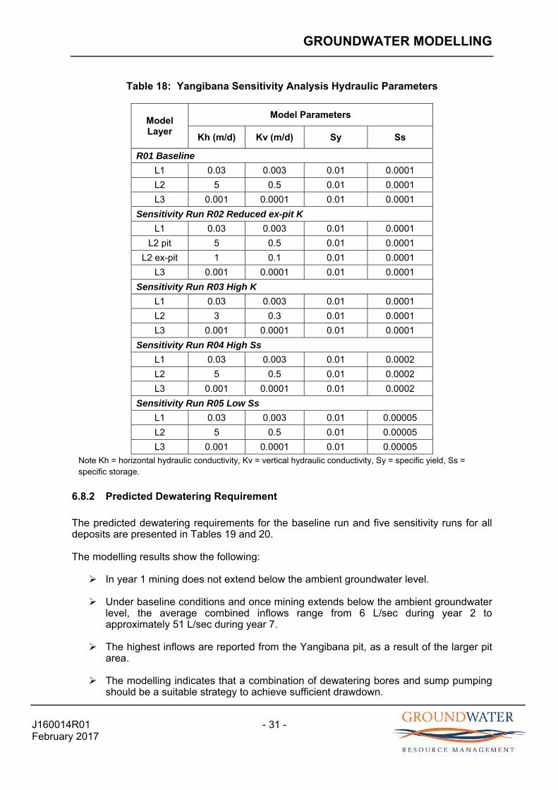
Table 18: Yangibana Sensitivity Analysis Hydraulic Parameters
Model Layer
Model Parameters
Kh (m/d) Kv (m/d) Sy Ss
R01 Baseline
L1 0.03 0.003 0.01 0.0001
L2 5 0.5 0.01 0.0001
L3 0.001 0.0001 0.01 0.0001
Sensitivity Run R02 Reduced ex-pit K
L1 0.03 0.003 0.01 0.0001
L2 pit 5 0.5 0.01 0.0001
L2 ex-pit 1 0.1 0.01 0.0001
L3 0.001 0.0001 0.01 0.0001
Sensitivity Run R03 High K
L1 0.03 0.003 0.01 0.0001
L2 3 0.3 0.01 0.0001
L3 0.001 0.0001 0.01 0.0001
Sensitivity Run R04 High Ss
L1 0.03 0.003 0.01 0.0002
L2 5 0.5 0.01 0.0002
L3 0.001 0.0001 0.01 0.0002
Sensitivity Run R05 Low Ss
L1 0.03 0.003 0.01 0.00005
L2 5 0.5 0.01 0.00005
L3 0.001 0.0001 0.01 0.00005
Note Kh = horizontal hydraulic conductivity, Kv = vertical hydraulic conductivity, Sy = specific yield, Ss = specific storage.
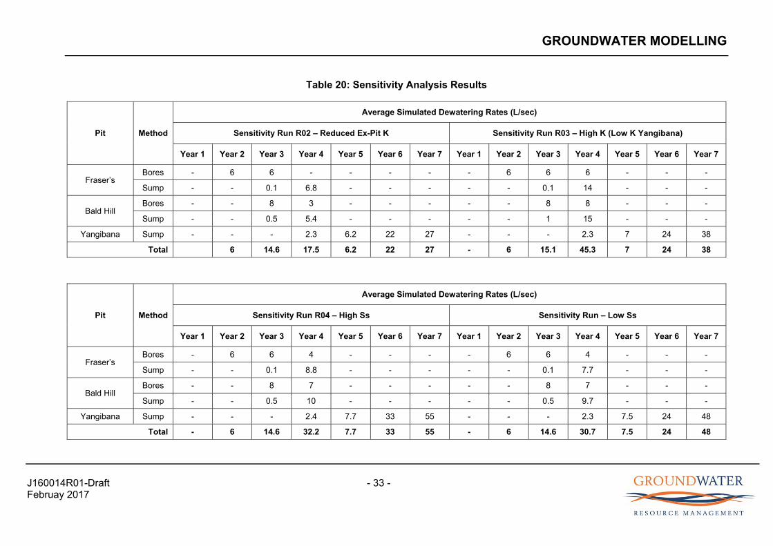
6.8.2 Predicted Dewatering Requirement
The predicted dewatering requirements for the baseline run and five sensitivity runs for all deposits are presented in Tables 19 and 20.
The modelling results show the following:
In year 1 mining does not extend below the ambient groundwater level.
Under baseline conditions and once mining extends below the ambient groundwater level, the average combined inflows range from 6 L/sec during year 2 to approximately 51 L/sec during year 7.
The highest inflows are reported from the Yangibana pit, as a result of the larger pit area.
The modelling indicates that a combination of dewatering bores and sump pumping should be a suitable strategy to achieve sufficient drawdown.

GROUNDWATER MODELLING
J160014R01 - 32 - February 2017
The model is moderately sensitive to changes in hydraulic conductivity, with inflows from year 4 reducing from 31.8 L/sec to 17.5 L/sec under low ex-pit K conditions and increasing to 45.3 L/sec under high K conditions.
It is important to note that the model does not allow for rainfall recharge, which is a conservative modelling approach with regard to drawdown impacts. Increased groundwater inflows following significant rainfall events are likely. For this reason it would be prudent to allow contingency for groundwater inflows of up to 50 L/sec following high rainfall events.
Additional contingency will also be necessary to account for surface water inflows (rainfall and runoff) following high rainfall events. It is understood Hastings is initiating a surface water assessment in early 2017, to assess potential surface water catchments and inflows.
Table 19: Predicted Base Case Dewatering Rates
Pit Method Average Simulated Dewatering Rate (L/sec)
Year 1 Year 2 Year 3 Year 4 Year 5 Year 6 Year 7
Fraser’s Bores - 6 6 4 - - -
Sump - - 0.1 8.5 - - -
Bald Hill Bores - - 8 7 - - -
Sump - - 0.5 10 - - -
Yangibana Sump - - - 2.3 7.5 25 51
Total - 6 14.6 31.8 7.5 25 51
GROUNDWATER MODELLING
J160014R01-Draft - 33 - Februay 2017
Table 20: Sensitivity Analysis Results
Pit Method
Average Simulated Dewatering Rates (L/sec)
Sensitivity Run R02 – Reduced Ex-Pit K Sensitivity Run R03 – High K (Low K Yangibana)
Year 1 Year 2 Year 3 Year 4 Year 5 Year 6 Year 7 Year 1 Year 2 Year 3 Year 4 Year 5 Year 6 Year 7
Fraser’s Bores - 6 6 - - - - - 6 6 6 - - -
Sump - - 0.1 6.8 - - - - - 0.1 14 - - -
Bald Hill Bores - - 8 3 - - - - - 8 8 - - -
Sump - - 0.5 5.4 - - - - - 1 15 - - -
Yangibana Sump - - - 2.3 6.2 22 27 - - - 2.3 7 24 38
Total 6 14.6 17.5 6.2 22 27 - 6 15.1 45.3 7 24 38
Pit Method
Average Simulated Dewatering Rates (L/sec)
Sensitivity Run R04 – High Ss Sensitivity Run – Low Ss
Year 1 Year 2 Year 3 Year 4 Year 5 Year 6 Year 7 Year 1 Year 2 Year 3 Year 4 Year 5 Year 6 Year 7
Fraser’s Bores - 6 6 4 - - - - 6 6 4 - - -
Sump - - 0.1 8.8 - - - - - 0.1 7.7 - - -
Bald Hill Bores - - 8 7 - - - - - 8 7 - - -
Sump - - 0.5 10 - - - - - 0.5 9.7 - - -
Yangibana Sump - - - 2.4 7.7 33 55 - - - 2.3 7.5 24 48
Total - 6 14.6 32.2 7.7 33 55 - 6 14.6 30.7 7.5 24 48

GROUNDWATER MODELLING
J160014R01 - 34 - February 2017
6.8.3 Predicted Groundwater Level Drawdown
The predicted groundwater level drawdown for the baseline runs at the end of mining are presented as contour plots in Figures 8 to 10. The plot shows the following:
The asymmetrical drawdown reflects the geometry of the aquifer, with the steep hydraulic gradient corresponding to the ironstone extending above the water table, whilst the drawdown propagates along strike and down-dip of the ironstone aquifer.
At the end of mining the predicted 5 m drawdown contour extends up to 1.5 km from the pit perimeter at Fraser’s, 1.25 km from the pit perimeter at Bald Hill and 2 km from the pit perimeter at Yangibana (Figures 8 to 10).
Steep hydraulic gradients are predicted in the fresh basement (HU3) beyond the outcropping ironstone, with the 5 m contour extending only about 500 m from the pit perimeter (Figure 8 to 10).
The groundwater drawdown contours suggest that other groundwater users in the area are not expected to be impacted by dewatering (Figure 11). The nearest identified other groundwater user (Yangibana Bore) is located 2.7 km from the predicted 5 m drawdown contour.

PIT LAKE MODELLING
J160014R01 - 35 - February 2017
7.0 PIT LAKE MODELLING
The pit lake model was developed using the generic systems modelling package GoldSim, which is ideally suited to coupled water and solute balance modelling. The model was run over a 500 year period to estimate pit lake conditions after mine closure.
The final mining depth in the three planned pits lies below the ambient groundwater level. At mine closure pumping will cease and the pits will start to flood forming a pit lake. Flooding will be primarily from the inflow of groundwater, which in conjunction with sporadic inflows from rainfall and runoff, will initially exceed losses from evaporation. This regime will be maintained until the combined inflow is balanced by the combined outflow, allowing for seasonal variability.
In the Gascoyne region, where evaporation far exceeds rainfall, the main drivers controlling the pit lake level will be groundwater inflow and evaporative outflow. Once the pit lake level stabilises one of two conditions are likely to develop. If the hydraulic conductivity of the groundwater systems associated with the pit lakes is sufficiently low, then a steep hydraulic gradient will be required to provide the necessary groundwater inflow to balance the evaporative loss. This will result in a depressed lake level and the development of a local groundwater sink (i.e. where the lake level lies below the groundwater level down-gradient of the pit), with no discharge of lake water to the groundwater environment.
Alternatively, if the hydraulic conductivity of the pit walls is sufficiently high then the hydraulic gradient needed to balance groundwater inflow against evaporative outflow will be low. In this instance, it is possible that the pit lake level will lie above the ambient groundwater level on the down-gradient side of the pit, thereby allowing pit lake water to discharge to the environment, forming a flow through cell.
If pit lake water is released, then there is a risk that any groundwater resources in the area could become impacted by mixing with pit water that may be contaminated.
7.1 Water Balance Set-Up
The GoldSim pit lake model includes three sub-models that simulate the development of pit void lakes in the three proposed pits. The model comprises the following components.
Pit lake storage volumes.
Inflows to the pits comprising:
groundwater inflows, which occur when the pit lake water level lies below the ambient groundwater level;
direct (incidental) rainfall onto the pit lakes;
rainfall runoff from the pit catchments into the pit void lakes.
Outflows from the pit comprising:
evaporation from the pit lakes;
groundwater outflows, which occur if the pit lake water level exceeds the ambient groundwater level.

PIT LAKE MODELLING
J160014R01 - 36 - February 2017
7.1.1 Pit Lake Storage Volume
The volume stored in the pit lake is estimated by the model based upon the total inflows and outflows to the lake over a time step, and the volume of the lake at the previous time step. At time zero (i.e. the start of the model run) the lake is assumed to have a nominal volume of 50 m3. GoldSim requires a volume at the start of the model run for the solute balance calculations.
The water balance equation used to calculate the stored volume is presented below.
Where Storagei = the pit lake volume at the current time step
Inflow = the total inflow to the pit lake
Outflow = the total outflow from the pit lake
Storagei-1 = the pit lake volume at the previous time step
7.1.2 Groundwater Inflows and Outflows
Estimation of seepage outflows and inflows from the pit lakes were calculated based upon the Dupuit equation for horizontal groundwater flow in an unconfined aquifer:
2
Where,
Q = seepage flow rate
P = pit perimeter length
K = hydraulic conductivity of the geological units adjacent to the pit lake
hB = difference in height between the ambient groundwater level and the base of aquifer (assumed to be equivalent to the pit floor elevation)
hA =difference in height between the pit lake water level and the base of pit lake (i.e. the lake depth)
L = flow path length.
All parameters in the equation, apart from hA, are applied as constants by the water balance. The perimeter length was estimated from mine plans provided by Snowden.
The height of the ambient groundwater level, which represents the natural water level unaffected by mining or groundwater production, was taken from monitoring data collected during the field investigation. Hydraulic conductivity and flow path length were based upon modelling studies completed during the dewatering assessment (Section 6.0) and adjusted during model verification.
The parameter values used in the water balance models are provided in Table 21.
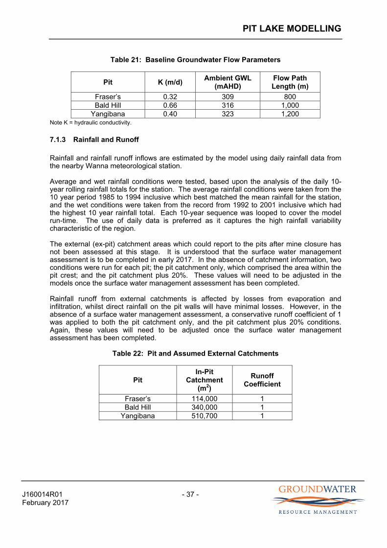
PIT LAKE MODELLING
J160014R01 - 37 - February 2017
Table 21: Baseline Groundwater Flow Parameters
Pit K (m/d) Ambient GWL
(mAHD) Flow Path Length (m)
Fraser’s 0.32 309 800 Bald Hill 0.66 316 1,000
Yangibana 0.40 323 1,200 Note K = hydraulic conductivity.
7.1.3 Rainfall and Runoff
Rainfall and rainfall runoff inflows are estimated by the model using daily rainfall data from the nearby Wanna meteorological station.
Average and wet rainfall conditions were tested, based upon the analysis of the daily 10-year rolling rainfall totals for the station. The average rainfall conditions were taken from the 10 year period 1985 to 1994 inclusive which best matched the mean rainfall for the station, and the wet conditions were taken from the record from 1992 to 2001 inclusive which had the highest 10 year rainfall total. Each 10-year sequence was looped to cover the model run-time. The use of daily data is preferred as it captures the high rainfall variability characteristic of the region.
The external (ex-pit) catchment areas which could report to the pits after mine closure has not been assessed at this stage. It is understood that the surface water management assessment is to be completed in early 2017. In the absence of catchment information, two conditions were run for each pit; the pit catchment only, which comprised the area within the pit crest; and the pit catchment plus 20%. These values will need to be adjusted in the models once the surface water management assessment has been completed.
Rainfall runoff from external catchments is affected by losses from evaporation and infiltration, whilst direct rainfall on the pit walls will have minimal losses. However, in the absence of a surface water management assessment, a conservative runoff coefficient of 1 was applied to both the pit catchment only, and the pit catchment plus 20% conditions. Again, these values will need to be adjusted once the surface water management assessment has been completed.
Table 22: Pit and Assumed External Catchments
Pit In-Pit
Catchment (m2)
Runoff Coefficient
Fraser’s 114,000 1 Bald Hill 340,000 1
Yangibana 510,700 1
PIT LAKE MODELLING
J160014R01 - 38 - February 2017
7.1.4 Evaporative Outflows
Evaporation losses are estimated by the model using the synthetic monthly evaporation rates estimated for the project area (Section 2.2), which uses the scaled mean of measured values at Paraburdoo and Learmonth. The monthly data is adjusted for pan to lake effects, using a coefficient of 0.7, and a salinity factor based on an empirical relationship developed by Turk (1970)1. The solute balance used to estimate the pit lake salinities is described in a later section below.
The adjusted evaporation rates were applied to the estimate area of the pit lakes, which were calculated from the relationship between lake volume and surface area at each time step (discussed in the following section).
7.1.5 Pit Geometry
The water balance uses the relationships between the pit volume (the independent variable), which is tracked by the model at each time step, and elevation and pit area (dependant variables) to estimate the groundwater-pit lake interaction, rainfall/runoff inflows and evaporative losses.
The pit geometry data (as provided by Snowden) is provided in Table 23.
1 LJ Turk 1970. “Evaporation of brine: a field study of the Bonneville salt flats, Utah”, August 1970. Water Resources Research 6(4), pp 1209-1215.
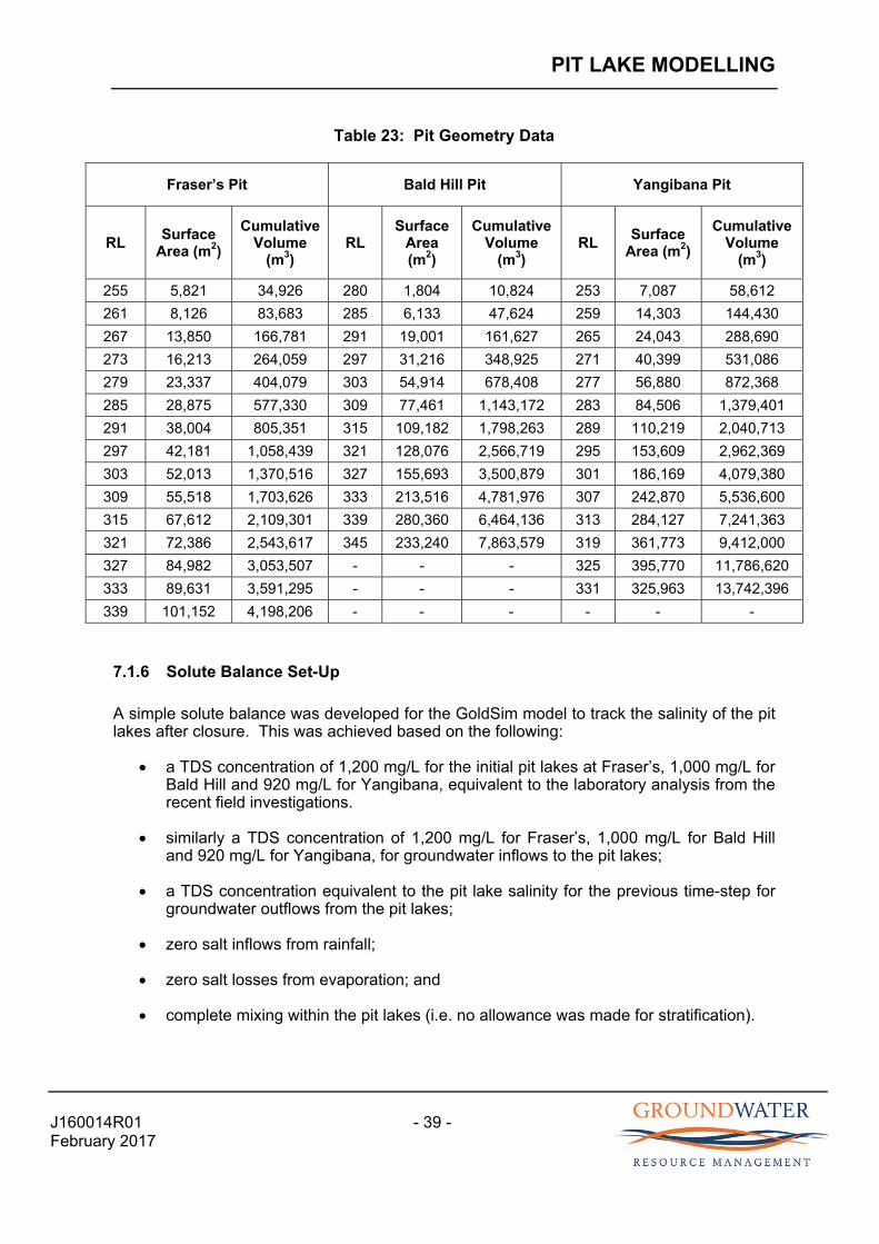
PIT LAKE MODELLING
J160014R01 - 39 - February 2017
Table 23: Pit Geometry Data
Fraser’s Pit Bald Hill Pit Yangibana Pit
RL Surface
Area (m2)
Cumulative Volume
(m3) RL
Surface Area (m2)
Cumulative Volume
(m3) RL
Surface Area (m2)
Cumulative Volume
(m3)
255 5,821 34,926 280 1,804 10,824 253 7,087 58,612
261 8,126 83,683 285 6,133 47,624 259 14,303 144,430
267 13,850 166,781 291 19,001 161,627 265 24,043 288,690
273 16,213 264,059 297 31,216 348,925 271 40,399 531,086
279 23,337 404,079 303 54,914 678,408 277 56,880 872,368
285 28,875 577,330 309 77,461 1,143,172 283 84,506 1,379,401
291 38,004 805,351 315 109,182 1,798,263 289 110,219 2,040,713
297 42,181 1,058,439 321 128,076 2,566,719 295 153,609 2,962,369
303 52,013 1,370,516 327 155,693 3,500,879 301 186,169 4,079,380
309 55,518 1,703,626 333 213,516 4,781,976 307 242,870 5,536,600
315 67,612 2,109,301 339 280,360 6,464,136 313 284,127 7,241,363
321 72,386 2,543,617 345 233,240 7,863,579 319 361,773 9,412,000
327 84,982 3,053,507 - - - 325 395,770 11,786,620
333 89,631 3,591,295 - - - 331 325,963 13,742,396
339 101,152 4,198,206 - - - - - -
7.1.6 Solute Balance Set-Up
A simple solute balance was developed for the GoldSim model to track the salinity of the pit lakes after closure. This was achieved based on the following:
a TDS concentration of 1,200 mg/L for the initial pit lakes at Fraser’s, 1,000 mg/L for Bald Hill and 920 mg/L for Yangibana, equivalent to the laboratory analysis from the recent field investigations.
similarly a TDS concentration of 1,200 mg/L for Fraser’s, 1,000 mg/L for Bald Hill and 920 mg/L for Yangibana, for groundwater inflows to the pit lakes;
a TDS concentration equivalent to the pit lake salinity for the previous time-step for groundwater outflows from the pit lakes;
zero salt inflows from rainfall;
zero salt losses from evaporation; and
complete mixing within the pit lakes (i.e. no allowance was made for stratification).
PIT LAKE MODELLING
J160014R01 - 40 - February 2017
7.2 Water Balance Modelling Results
A run time of 500 years was adopted for the water balance model simulations, using a one day time step.
Twelve model runs were completed, comprising:
three base case runs (one per pit) using the pit only catchment and expected conditions
three sensitivity runs (one per pit) using the pit only catchment and high rainfall conditions
three sensitivity runs (one per pit) using the pit plus 20% catchment and expected conditions
three sensitivity runs (one per pit) using the pit plus 20% catchment high rainfall conditions
The groundwater inflow rates predicted by the water balance for the three pits was verified by comparing the inflow rate against the dewatering requirements estimated in the groundwater flow models. The water balance inflow rates approximate those derived from the dewatering assessment at the end of mining.

PIT LAKE MODELLING
J160014R01 - 41 - February 2017
Table 24: Model Runs
Run No Pit Rainfall Catchment Run Type
01 Fraser’s Average Pit Only Baseline
02 Fraser’s Wet Pit Only Sensitivity
03 Fraser’s Average Pit plus 20% Sensitivity
04 Fraser’s Wet Pit plus 20% Sensitivity
05 Bald Hill Average Pit Only Baseline
06 Bald Hill Wet Pit Only Sensitivity
07 Bald Hill Average Pit plus 20% Sensitivity
08 Bald Hill Wet Pit plus 20% Sensitivity
09 Yangibana Average Pit Only Baseline
10 Yangibana Wet Pit Only Sensitivity
11 Yangibana Average Pit plus 20% Sensitivity
12 Yangibana Wet Pit plus 20% Sensitivity
The predicted pit lake water levels for model Runs 01 to 12 are presented as time series plots in Figures 12 to 14. The figures also present the adopted ambient groundwater level at the deposits. The pit lake water levels and lake residual drawdowns2 for the 12 model runs are presented in Table 17. The figures and table show the following:
All model runs show a similar pattern following the cessation of mining:
A rapid pit lake level rise over the initial 10 years when groundwater inflow rates far exceed evaporation rates, because of the high groundwater hydraulic gradient and the comparatively small lake area available for evaporation.
The rate of rise reduces between 10 and 15 years after cessation of dewatering due to increased evaporation rates, because of the expanded pit lake area as the pit fills, and the reduced groundwater inflow rate in response to the lowering of the groundwater gradient towards the pit.
2 The residual drawdown represents the vertical distance from the ambient groundwater level to the pit lake level. Positive values indicate the lake will form a groundwater sink, while negative values, where lake levels lie above the surrounding groundwater level, suggests seepage from the pit lake to the groundwater system will occur.
PIT LAKE MODELLING
J160014R01 - 42 - February 2017
The pit lake water levels equilibrate after 20 years as the falling groundwater and rainfall inflows are balanced by the evaporative losses.
By the end of the 500 year model run, the pit lake levels have stabilised, with minor seasonal and annual variations in response to variation in rainfall and evaporation.
For the baseline condition the final predicted pit lake level ranges from 300.9 mAHD in Fraser’s, to 311.1 mAHD in Bald Hill, to 311.5 mAHD in Yangibana, which gives a residual drawdown range of 8.0 m (Fraser’s), to 4.9 m (Bald Hill), to 11.5 m (Yangibana), indicating that all pits act as groundwater sinks under baseline conditions.
For the sensitivity analyses relating to wet years (Runs 02, 04, 06, 08, 10, 12), the residual drawdown ranges from 2.5 m (Bald Hill) to 10.4 m (Yangibana), indicating that the pits continue to act as groundwater sinks under high rainfall conditions.
The model also provides an estimate of TDS concentrations post-closure, based upon evaporative concentration in the pit lakes. The results indicate that after 500 years post closure the TDS in Fraser’s increase from 1,200 mg/L to about 44,000 mg/L TDS, in Bald Hill increase from 1,000 mg/L to about 48,000 mg/L TDS, and in Yangibana increase from 920 mg/L to about 37,000 mg/L TDS.
The results of the pit lake modelling indicate that the risk of impact (i.e. discharge of lake water) to the groundwater environment post closure is low. However, it should be noted that the residual drawdown is a function of the ex-pit catchment parameters, i.e. pits with larger ex-pit catchments and lower rainfall coefficients report higher final predicted pit lake levels and corresponding lower residual drawdowns. Therefore the pit lake modelling will require re-running once the ex-pit catchment parameters are established as part of the pending surface water management assessment for the Project.
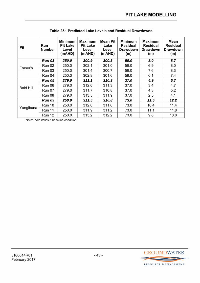
PIT LAKE MODELLING
J160014R01 - 43 - February 2017
Table 25: Predicted Lake Levels and Residual Drawdowns
Pit Run Number
Minimum Pit Lake
Level (mAHD)
Maximum Pit Lake
Level (mAHD)
Mean Pit Lake Level
(mAHD)
Minimum Residual
Drawdown (m)
Maximum Residual
Drawdown (m)
Mean Residual
Drawdown (m)
Fraser’s
Run 01 250.0 300.9 300.3 59.0 8.0 8.7 Run 02 250.0 302.1 301.0 59.0 6.9 8.0 Run 03 250.0 301.4 300.7 59.0 7.6 8.3 Run 04 250.0 302.9 301.6 59.0 6.1 7.4
Bald Hill
Run 05 279.0 311.1 310.3 37.0 4.9 5.7 Run 06 279.0 312.6 311.3 37.0 3.4 4.7 Run 07 279.0 311.7 310.8 37.0 4.3 5.2 Run 08 279.0 313.5 311.9 37.0 2.5 4.1
Yangibana
Run 09 250.0 311.5 310.8 73.0 11.5 12.2 Run 10 250.0 312.6 311.6 73.0 10.4 11.4 Run 11 250.0 311.9 311.2 73.0 11.1 11.8 Run 12 250.0 313.2 312.2 73.0 9.8 10.8
Note: bold italics = baseline condition
DEWATERING STRATEGY
J160014R01 - 44 - February 2017
8.0 DEWATERING STRATEGY
The inflow rates predicted by the groundwater flow models indicate dewatering of the proposed pits will be best achieved by a combination of ex-pit dewatering bores and sump pumping methods.
Sufficient additional contingency of at least 50 L/sec should be considered to allow for short term, higher than anticipated groundwater inflow rates upon interception of additional water bearing features in the fresh bedrock, and to manage increases in groundwater inflows following high rainfall events. Further contingency will need to be considered to account for surface water inflows as a result of rainfall and runoff to the pits.
The dewatering bores should be positioned into a thick (preferably greater than 10 m) sequence of ironstone, and located just outside the crest of the pits, on the down dip side. One to two dewatering bores would be suitable for each of Fraser’s and Bald Hill, and two to three bores would be suitable for Yangibana. Additional dewatering bores could be considered if higher than predicted inflow rates are observed during operations.
The test bores FRW03 and BHW05 are suitably located as dewatering bores. However given that they were constructed for testing purposes only, using uPVC casing, they may not withstand the pressure of blasting during mining. The test bores will be suitable during the construction phase but will likely require replacement or refurbishment prior to mining.
The dewatering bores should be constructed using 6” schedule 40 steel casing (7.1 mm wall thickness). The steel casing should be slotted across the main aquifer zone (as per the test bore construction), with the bore annulus gravel packed to just below the surface. The annulus will need to be sealed at the surface, with cement grout or bentonite, to prevent surface water ingress.
It is recommended the dewatering bores are installed at least 6 months prior to mining to achieve sufficient drawdown. However the bores can be operated prior to this, to provide additional make-up water to meet the Project demand if necessary (discussed further in Section 9.0), which will further aid mine dewatering.
Sump pumping will require ongoing management during the operational life of the pits. Sumps should be strategically located at low points along the pit floor.
All dewatering discharge will be transferred to a process water dam at the surface for use by the operation for dust suppression and mineral processing. At the predicted dewatering rates there should be no requirement to discharge mine water to the environment.
A monitoring programme will be required during mining to help assess the impacts upon the groundwater environment from groundwater abstraction as a result of dewatering activities. As part of the monitoring programme a network of monitoring bores will need to be installed to provide an indication of drawdown impacts upon the surrounding groundwater system. An operating strategy will be required as part of the conditions of a future groundwater abstraction (5C) licence, based upon the DoW guidelines (Operational Policy 5.08). A monitoring programme and operating strategy should be prepared upon completion of the Stage II DFS study.
WATER SUPPLY OPTIONS
J160014R01 - 45 - February 2017
9.0 WATER SUPPLY OPTIONS
The Project’s estimated total water demand is in the order of 2.5 GL/annum (79.3 L/sec) of fresh to brackish quality groundwater, for the purposes of processing, dust suppression and domestic / potable use.
As discussed in Section 6.8.1, mine dewatering is anticipated to provide a water supply for the project after year 2, with average estimated dewatering rates ranging from 6 L/sec during year 2 to approximately 51 L/sec during year 7. Consequently an alternate water supply will be necessary to provide the full demand (79.3 L/sec) for the first year of operation, and part of the demand for the remainder of the LoM.
Additional water supply options for the Project include:
Extended use of dewatering bores. It is recommended (Section 7.0) that the dewatering bores are operated at least 6 months prior to mining to achieve sufficient drawdown. However, at Yangibana, and to a lesser extent Fraser’s, the dewatering bores could be operated from year 1, which could provide an additional supply of about 20 to 30 L/sec during the first few years of mining. Additional field investigations will be necessary to confirm suitable bore locations (other than at FRW03 and BHW05).
Sacrificial bore at Yangibana. During the Stage I field investigations, a location for a potential sacrificial bore was identified (at YWRC057) within the pit area. The drill-hole yielded 8 L/sec during airlift recovery testing and could potentially provide a supply of 10 to 15 L/sec for years 1 to 3, prior to the commencement of mining at Yangibana.
Extended use of sump pumping. Groundwater abstraction from the Fraser’s and Bald Hill pits could continue after mining, providing an additional water supply during years 5 to 7. Groundwater modelling indicates that groundwater inflows to pit at the end of mining are about 10 L/sec at Fraser’s and 14 L/sec at Bald Hill, potentially providing an additional 24 L/sec during the latter stages of the Project.
Water supply bores Auer North. Auer North is located approximately 5 km west of Fraser’s (Figure 11) and anecdotally reported groundwater inflows similar to those reported in Bald Hill. Further field investigations would be necessary to confirm the water supply potential from this area. However, anecdotal information suggests there is the potential for 1 to 2 bores at about 8 L/sec per bore. The proximity of Auer North to Fraser Well will need to be considered in the Stage II study.
Water supply borefield Western Belt. Hastings has identified an area of approximately 12 km of ironstone strike length, referred to as the Western Belt (Figure 11), extending east of Yangibana. Resource drilling has indicated similar characteristics (i.e. thick sequence of fractured and vuggy ironstone) to those observed at Yangibana, suggesting the Belt may be suitable for a borefield. A borefield of up to 10 bores along the Belt could provide up to 60 L/sec for the duration of the Project. However additional field investigations will be necessary to confirm the water supply potential of this area.
Palaeochannel water supply borefield. The WASANT Palaeovalley Map, produced by the National Water Commission, indicates that the Lyons Palaeovalley lies to the west of Yangibana and to the south of Bald Hill and Fraser’s. Whilst there is

WATER SUPPLY OPTIONS
J160014R01 - 46 - February 2017
very little data on likely yields from palaeochannel aquifers in the immediate area, palaeochannel aquifers provide reliable yields in other regions. The benefit of a palaeochannel borefield for the Project is that it removes the reliance on the ironstone aquifer, which potentially has limited storage. However, groundwater quality in palaeochannel aquifers are typically poorer; there is the potential for interaction with GDE’s, and additional tenure may need to be acquired. Further investigations would be necessary, should Hastings wish to pursue this option, which would likely include an initial assessment of publicly available geophysical surveys to identify target transects, followed by further ground surveys (if necessary) and aircore drilling to identify the deepest part of the palaeochannel.
It is expected that the Project’s water supply demand can be met from a combination of dewatering and some of the above-mentioned additional sources. However further hydrogeological investigations would be necessary to confirm this.
SUMMARY AND CONCLUSIONS
J160014R01 - 47 - February 2017
10.0 SUMMARY AND CONCLUSIONS
Hastings owns the Yangibana Rare Earths Project (the Project), located approximately 270 km east north-east of Carnarvon, in the Upper Gascoyne region of Western Australia.
The project has an estimated annual water demand of up to 2.5 GL/annum (79.3 L/sec), for the purposes of mineral processing, dust suppression and camp / potable supply (via reverse osmosis treatment).
The results of the Stage I study are as follows:
The results of the exploration drilling confirmed modest groundwater inflows associated with the ironstone dykes, and identified suitable test bore locations at Fraser’s and Bald Hill.
The results of the hydraulic testing indicated; airlift yields ranged from 0.015 L/sec to 8 L/sec; three test locations reported low permeability conditions (hydraulic conductivity below 0.1 m/day); three test locations reported low to modest permeability conditions (hydraulic conductivity between 0.1 and 1 m/day); and six test locations reported modest permeability conditions (hydraulic conductivity above 1 m/day).
Two test production bores were installed (FRW03 at Fraser’s and BHW05 at Bald Hill), intercepting the ironstone aquifer, down-dip from the proposed pits. The bores were constructed using 155 mm Class 9 uPVC casing to depths of 95.2 and 104 m respectively.
Three bores were test pumped (FRW03, BHW05 and the existing drilling supply bore YGWB03). Testing comprised a 3 to 4 hour step test and 48 hour constant rate test, and recovery test. The test pumping indicated drawdown patterns consistent with a semi-confined aquifer, with barrier boundary conditions observed in the Fraser’s and Bald Hill bores, indicative of a fractured rock environment whereby smaller fractures are drained during testing. The results indicate a hydraulic conductivity range of 2.5 to 5.6 m/day, which is consistent with the hydraulic testing results.
Estimated long term duty rates for FRW03 are 7 L/sec for peak use, and 6 L/sec for long term operational use, and for BHW05 are 10 L/sec for peak use, and 8 L/sec for long term operational use. YGWB03 is low yielding and probably unsuitable for a long term operational supply.
It must be understood that the ironstone aquifer potentially has limited storage, and sufficient water supply contingency will be necessary for the Project to account for this.
The groundwater salinity in the three production bores varies from about 920 mg/L TDS at Yangibana, 1,000 mg/L TDS at Bald Hill, and 1,200 mg/L TDS at Fraser’s.
Groundwater samples have been collected and submitted to ANSTO for isotope analysis to provide an indication of groundwater age. Results are expected in April 2017.
SUMMARY AND CONCLUSIONS
J160014R01 - 48 - February 2017
The groundwater level along the deposits range from about 309 mRL at Fraser’s to 316 mRL at Bald Hill and 323 mRL at Yangibana. The groundwater flow direction is south south-west towards the Lyons River.
The results of the field testing programme were used to construct a 3D groundwater flow model for the deposits and surrounding groundwater system to simulate the impacts upon the groundwater environment from mining below the water table. Sensitivity analyses were run to assess the implications of varying hydraulic properties. The results of the modelling indicate:
Under baseline conditions the average inflows range from 0 L/sec during the first year to 51 L/sec during year 7. Additional contingency of about 50 L/sec will be necessary to allow for short term, higher than anticipated inflow rates. Additional contingency will be necessary to manage incidental rainfall into the pit void and rainfall runoff.
The drawdown extents at the end of mining are asymmetrical which reflects the geometry of the aquifer, with the steep hydraulic gradient corresponding to the ironstone extending above the water table, whilst the drawdown propagates along strike and down-dip of the ironstone.
At the end of mining the predicted 5 m drawdown contour extends up to 1.5 km from the pit perimeter at Fraser’s, 1.25 km from the pit perimeter at Bald Hill and 2 km from the pit perimeter at Yangibana.
Steep hydraulic gradients are predicted in the fresh basement beyond the outcropping ironstone, with the 5 m contour extending only about 500 m from the pit perimeter.
The groundwater drawdown contours suggest that other groundwater users in the area are not expected to be impacted by dewatering.
A pit lake model was developed for each pit using the systems modelling package GoldSim. The models were run over a 500 year period to estimate pit lake conditions after mine closure. The results indicate that the risk of impact (i.e. discharge of lake water) to the groundwater environment post closure is low. However pit catchment areas have not yet been characterised for the project, and so the models were based on a nominal ex-pit catchment size of 20% of the pit area. Considering that the residual drawdown in the pits is a function of the ex-pit catchment parameters, i.e. pits with larger ex-pit catchments and lower rainfall coefficients report higher final predicted pit lake levels and corresponding lower residual drawdowns, the pit lake modelling will require re-running once the ex-pit catchment parameters are established.
The recommended dewatering strategy for the Project, based upon the groundwater inflow rates predicted by the modelling, is a combination of ex-pit dewatering bores and sump pumping. One to two dewatering bores would be suitable for each of Fraser’s and Bald Hills, and two to three bores would be suitable for Yangibana. Additional dewatering bores could be considered if higher than predicted inflow rates are observed during operations. The dewatering bores should be constructed at least 6 months prior to mining to achieve sufficient drawdown, and constructed using 6“ mild steel casing to prevent damage during blasting. Sump pumping will be required in all pits for the duration of mining.

SUMMARY AND CONCLUSIONS
J160014R01 - 49 - February 2017
The Project will require additional water supply sources to supplement the dewatering supply and meet the Projects total water demand of 2.5 GL/annum (79.3 L/sec). Additional water supply options have been identified which include extended use of dewatering bores and sump pumping; a sacrificial bore at Yangibana; water supply bore/s at Auer North; a water supply borefield in the Western Belt; or a palaeochannel water supply borefield. The benefit of a palaeochannel borefield for the Project is that it removes the reliance on the ironstone aquifer, which potentially has limited storage. However, groundwater quality in palaeochannel aquifers are typically poorer; there is the potential for interaction with GDE’s, and additional tenure may need to be acquired. Further investigations will be necessary to confirm additional water supply sources for the Project.
Groundwater Resource Management Pty Ltd
Kathy McDougall Rob Garnham
SENIOR HYDROGEOLOGIST PRINCIPAL HYDROGEOLOGIST F:\J160014_YANGIBANA\REPORT\FINAL\J160014R01_FINAL.DOCX
This report has been printed on paper that contains a proportion of recycled material as a gesture of Groundwater Resource
Management’s commitment to sustainable management of the environment.

Yangibana DFS Stage I (J160014R01)
Hastings Technology Minerals Ltd
FIGURE 1KM Jan 17
SITE LOCATION PLAN
FILE:\\G:\Jobs2016\J160014_YangibanaFS/figures/other/locplan.pptx
YangibanaRare Earths
Project

412,000 414,000 416,000 418,000 420,000 422,000 424,000 426,000 428,000 430,000 432,000
Easting (MGA94 Zone 50)
7,342,000
7,344,000
7,346,000
7,348,000
7,350,000
7,352,000
7,354,000
7,356,000
7,358,000
7,360,000
7,362,000
7,364,000
7,366,000
7,368,000
7,370,000
7,372,000N
orth
ing
(MG
A94
Zon
e 50
)
YANGIBANA
FRASERS
BALD HILL
LEGEND
Proposed Pits

Yangibana
Bald Hills
Fraser's
BENBAGEON WELL (W16)
BOOGARDI BORE (W17)
DINGO WELL (W18)
CARDIBAR BORE W12
GAP BORE (E17)
PIMBIANA BORE W10
HENDERSON BORE W11
(W13) WALLABY BORE
ROADSIDE BORE (W14)
FRASER WELL F1
E15 CONTESSE WELL
E16 RED HILL BORE
YANGIBANA BORE F2
Edmund HST
Minga Well
Contessi Bore
Edmund Well
Frasers Well
Yangibana Bore
Woodsys Bore
Red Hill 2
405,000 410,000 415,000 420,000 425,000 430,000 435,000 440,000 445,000
Easting (MGA94 Zone 50)
7,350,000
7,355,000
7,360,000
7,365,000
7,370,000
Nor
thin
g (M
GA
94 Z
one
50)
LEGEND
WIR Bores
Bores Sampled During PFS
Proposed Pits
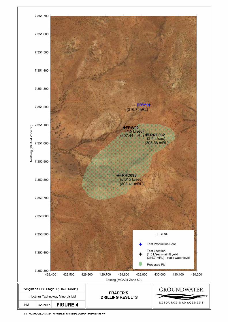
FRW02
FRRC082
FRRC098
(1.5 L/sec)
(3.4 L/sec)
(0.015 L/sec)
(316.7 mRL)
(307.44 mRL)
(303.36 mRL)
(303.41 mRL)
FRW1
429,400 429,500 429,600 429,700 429,800 429,900 430,000 430,100 430,200
Easting (MGA94 Zone 50)
7,350,300
7,350,400
7,350,500
7,350,600
7,350,700
7,350,800
7,350,900
7,351,000
7,351,100
7,351,200
7,351,300
7,351,400
7,351,500
7,351,600
7,351,700
No
rth
ing
(M
GA
94
Zo
ne
50
)
LEGEND
Test Production Bore
Test Location(1.5 L/sec) - airlift yeild(316.7 mRL) - static water level
Proposed Pit

BHW01
BHW02
BHW03
BHW04
BHRC082
BHRC161
BHRC097
BHRC095
(3.9 L/sec)
(1.8 L/sec)
(0.14 L/sec)
(2 L/sec)
(3 L/sec)
(0.8 L/sec)
(0.33 L/sec)
(320.7 mRL)
(320 mRL)
(320.65 mRL)
(320.18 mRL)
(322.77 mRL)
(317.73 mRL)
(307.02 mRL)
(307.98 mRL)
BHW05
427,800 428,000 428,200 428,400 428,600 428,800
Easting (MGA94 Zone 50)
7,355,200
7,355,400
7,355,600
7,355,800
7,356,000
7,356,200
7,356,400
7,356,600
7,356,800
7,357,000
7,357,200
Nor
thin
g (M
GA
94 Z
one
50)
LEGEND
Test Production Bore
Test Location(3.9 L/sec) - airlift yield(320.7 mRL) - static water level
Proposed Pits
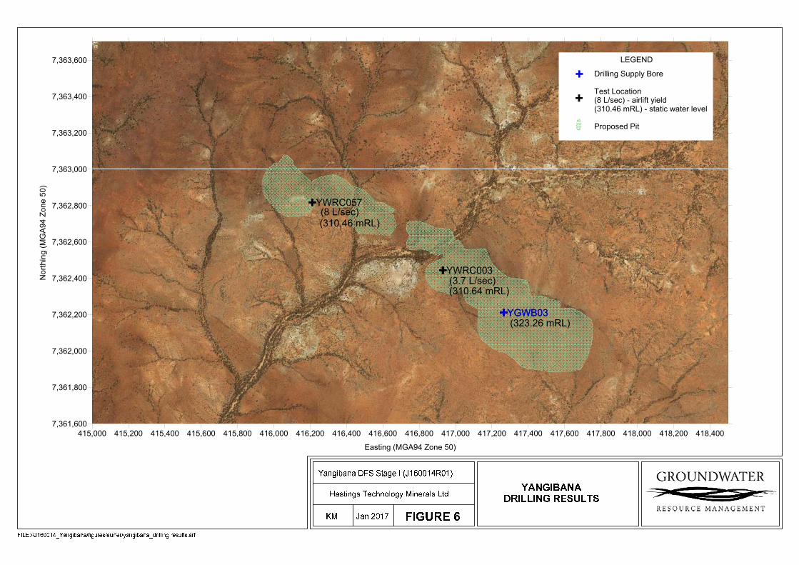
YWRC003
YWRC057
YGWB03
(3.7 L/sec)
(8 L/sec)
(310.64 mRL)
(310.46 mRL)
(323.26 mRL)YGWB03
415,000 415,200 415,400 415,600 415,800 416,000 416,200 416,400 416,600 416,800 417,000 417,200 417,400 417,600 417,800 418,000 418,200 418,400
Easting (MGA94 Zone 50)
7,361,600
7,361,800
7,362,000
7,362,200
7,362,400
7,362,600
7,362,800
7,363,000
7,363,200
7,363,400
7,363,600
Nor
thin
g (M
GA
94 Z
one
50)
LEGEND
Drilling Supply Bore
Test Location(8 L/sec) - airlift yield(310.46 mRL) - static water level
Proposed Pit
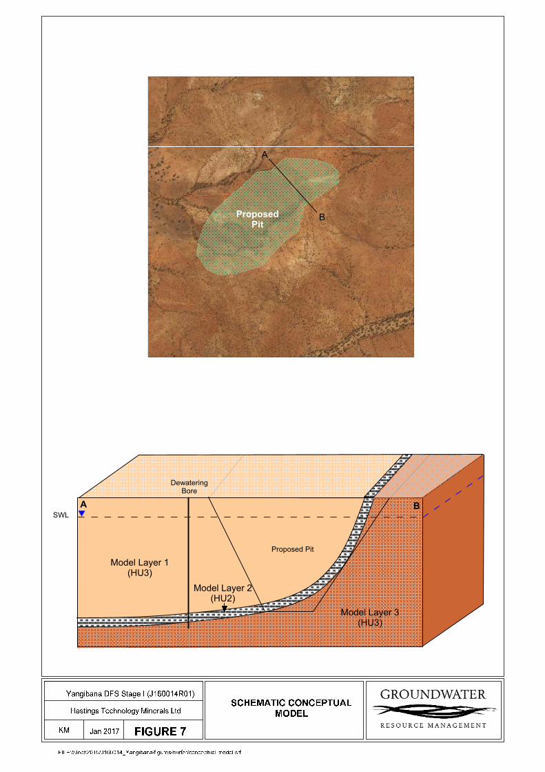
A
BProposedPit
DewateringBore
A B
Model Layer 1(HU3)
Model Layer 2(HU2)
Model Layer 3(HU3)
SWL
Proposed Pit

FRW1
5 m
5 m
5 m
5 m
5 m
5 m
10 m
10 m
10 m
10 m
15 m
15 m
15 m
20 m
20 m
20 m
25 m
25 m
30 m
30 m
35 m
40 m
428,000 428,500 429,000 429,500 430,000 430,500
Easting (MGA94 Zone 50)
7,349,500
7,350,000
7,350,500
7,351,000
7,351,500
7,352,000
7,352,500
7,353,000
7,353,500N
ort
hin
g (
MG
A9
4 Z
on
e 5
0)
LEGEND
Simulated Drawdon ContoursEnd of Mining
Production Bore
Proposed Pit

5 m
5 m
5 m
5 m
5 m
5 m
5 m10 m
10 m
10 m
10 m
15 m
15 m
15 m
20 m
20 m
25 m BHW05
426,500 427,000 427,500 428,000 428,500 429,000
Easting (MGA94 Zone 50)
7,354,500
7,355,000
7,355,500
7,356,000
7,356,500
7,357,000
7,357,500
7,358,000N
orth
ing
(MG
A94
Zon
e 50
)
LEGEND
Simulated Drawdown ContousEnd of Mining
Production Bore
Proposed Pits
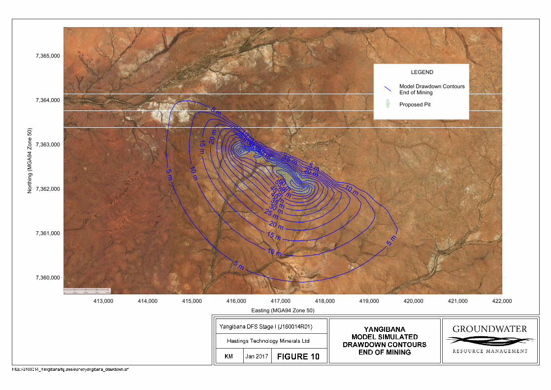
5 m
5 m
5 m
5 m
5 m
10 m
10 m
10 m
10 m
15 m
15
m
15 m
20 m
20 m
20 m
25 m
25 m
30 m
30 m
35 m
35 m
40 m
40 m
45 m50 m
55 m
60 m
413,000 414,000 415,000 416,000 417,000 418,000 419,000 420,000 421,000 422,000
Easting (MGA94 Zone 50)
7,360,000
7,361,000
7,362,000
7,363,000
7,364,000
7,365,000
Nor
thin
g (M
GA
94 Z
one
50)
LEGEND
Model Drawdown ContoursEnd of Mining
Proposed Pit
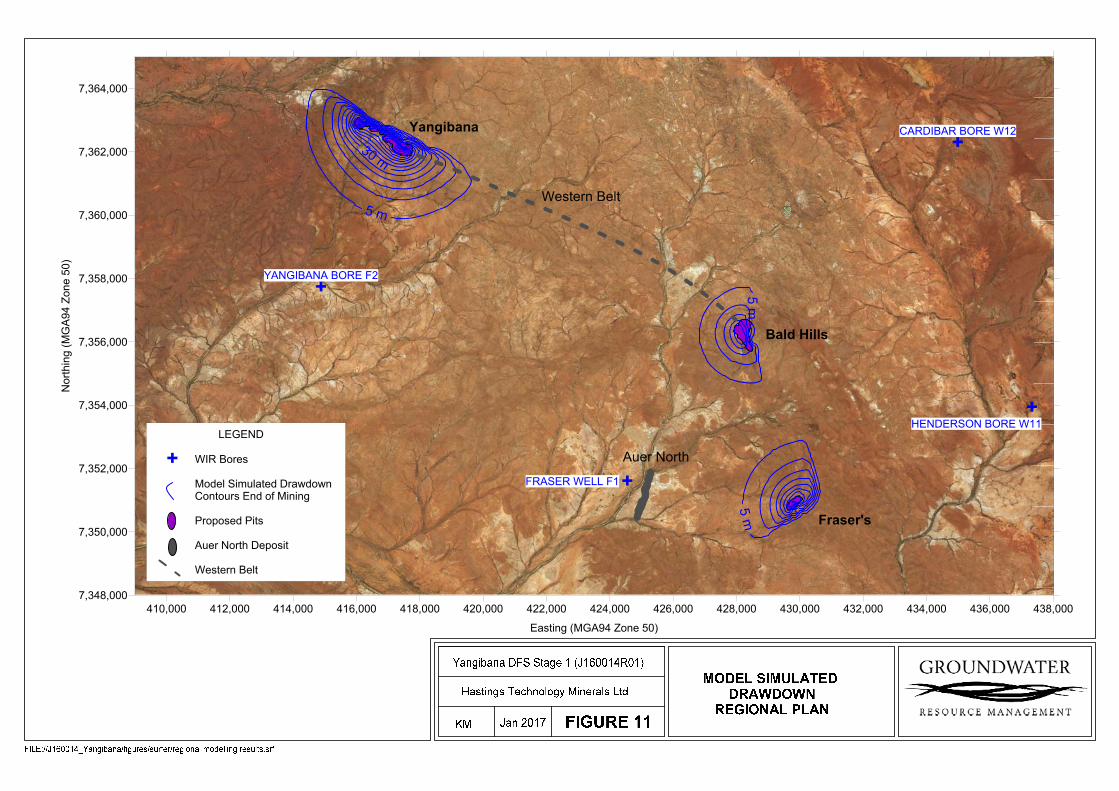
Yangibana
Bald Hills
Fraser's
CARDIBAR BORE W12
HENDERSON BORE W11
FRASER WELL F1
YANGIBANA BORE F2
5 m
5 m
5 m
30 m
410,000 412,000 414,000 416,000 418,000 420,000 422,000 424,000 426,000 428,000 430,000 432,000 434,000 436,000 438,000
Easting (MGA94 Zone 50)
7,348,000
7,350,000
7,352,000
7,354,000
7,356,000
7,358,000
7,360,000
7,362,000
7,364,000
Nor
thin
g (M
GA
94 Z
one
50)
LEGEND
WIR Bores
Model Simulated DrawdownContours End of Mining
Proposed Pits
Auer North Deposit
Western Belt
Auer North
Western Belt
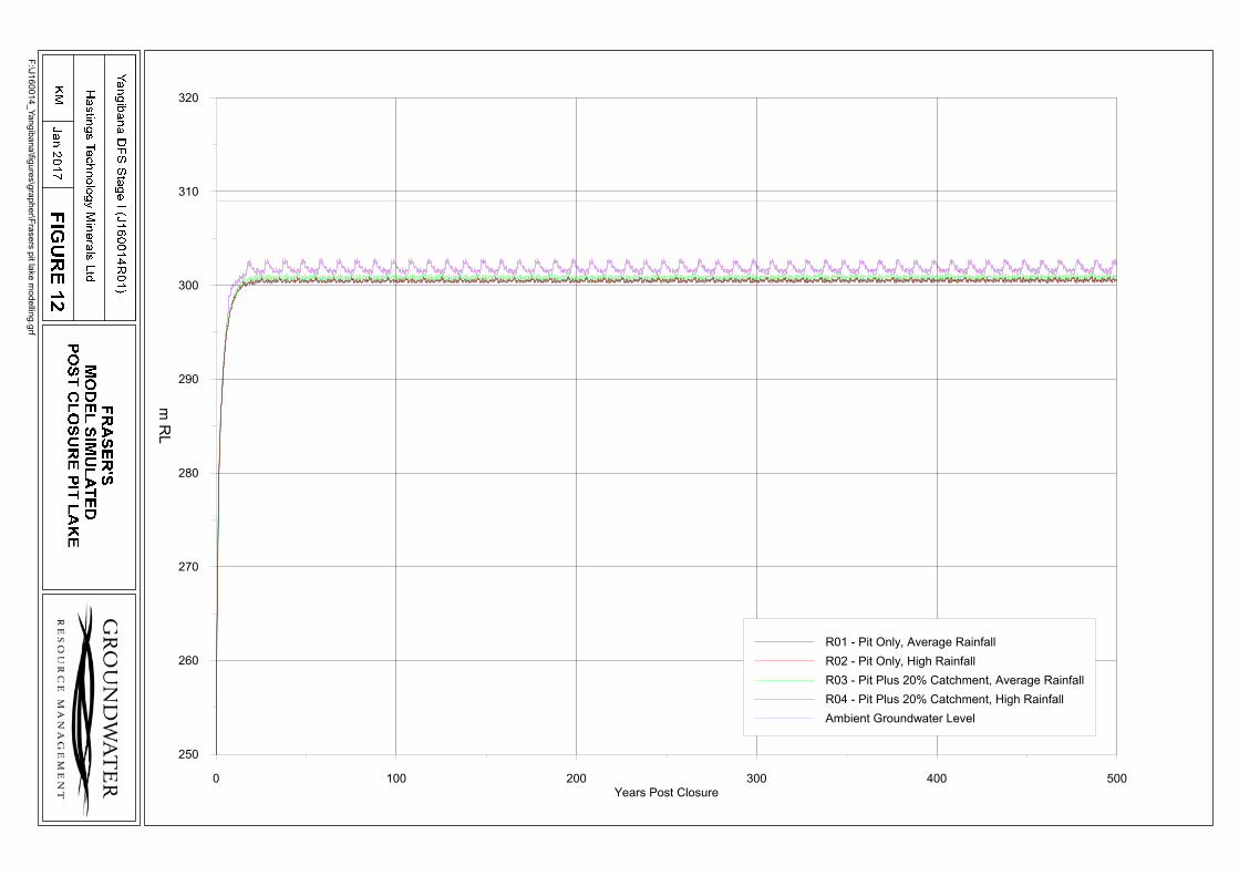
F:\J1
60014_Yangibana\figures\grapher\F
rasers pit lake modelling
.grf
0 100 200 300 400 500Years Post Closure
250
260
270
280
290
300
310
320
m R
L
R01 - Pit Only, Average Rainfall
R02 - Pit Only, High Rainfall
R03 - Pit Plus 20% Catchment, Average Rainfall
R04 - Pit Plus 20% Catchment, High Rainfall
Ambient Groundwater Level
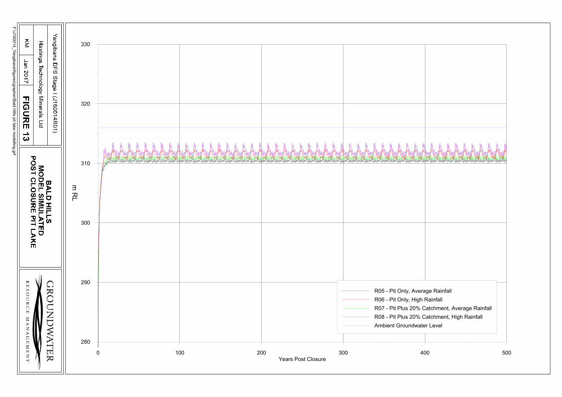
F:\J1
60014_Yangibana\figures\grapher\B
ald Hills pit lake m
odelling.grf
0 100 200 300 400 500Years Post Closure
280
290
300
310
320
330
m R
L
R05 - Pit Only, Average Rainfall
R06 - Pit Only, High Rainfall
R07 - Pit Plus 20% Catchment, Average Rainfall
R08 - Pit Plus 20% Catchment, High Rainfall
Ambient Groundwater Level
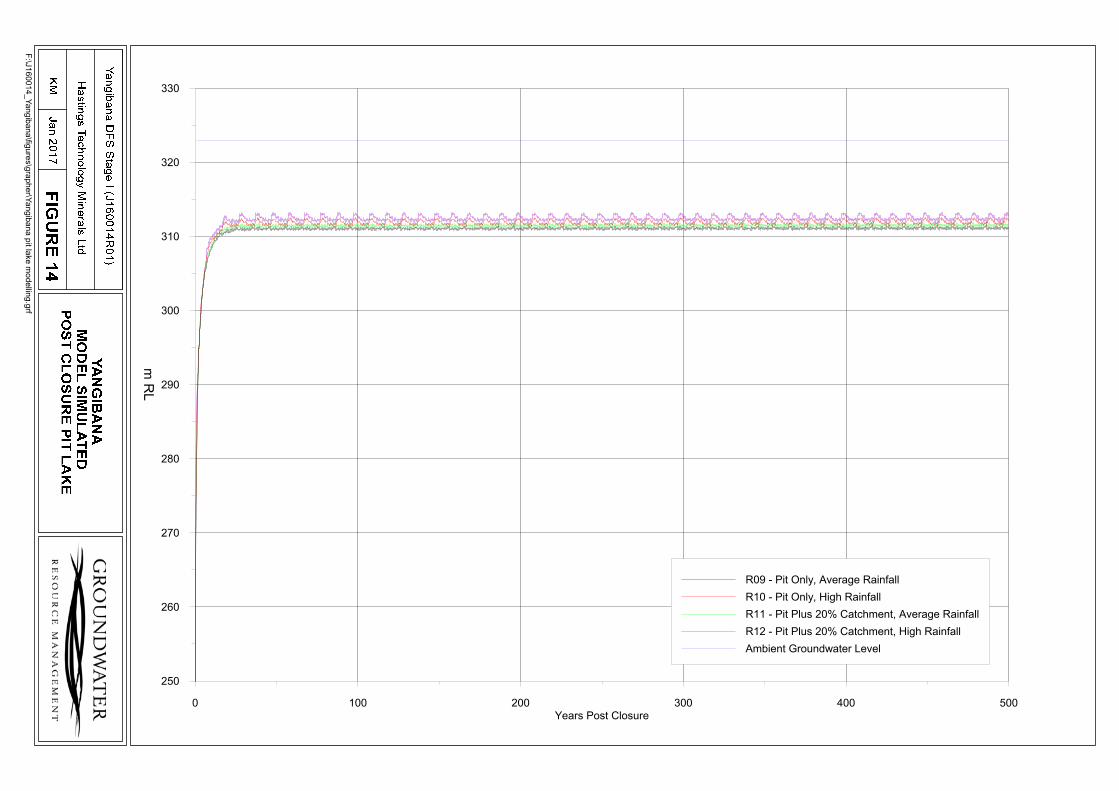
F:\J1
60014_Yangibana\figures\grapher\Y
angibana pit lake modelling.grf
0 100 200 300 400 500Years Post Closure
250
260
270
280
290
300
310
320
330
m R
L
R09 - Pit Only, Average Rainfall
R10 - Pit Only, High Rainfall
R11 - Pit Plus 20% Catchment, Average Rainfall
R12 - Pit Plus 20% Catchment, High Rainfall
Ambient Groundwater Level

J160014R01 A-1 February 2017
APPENDIX A
BoM GDE Report
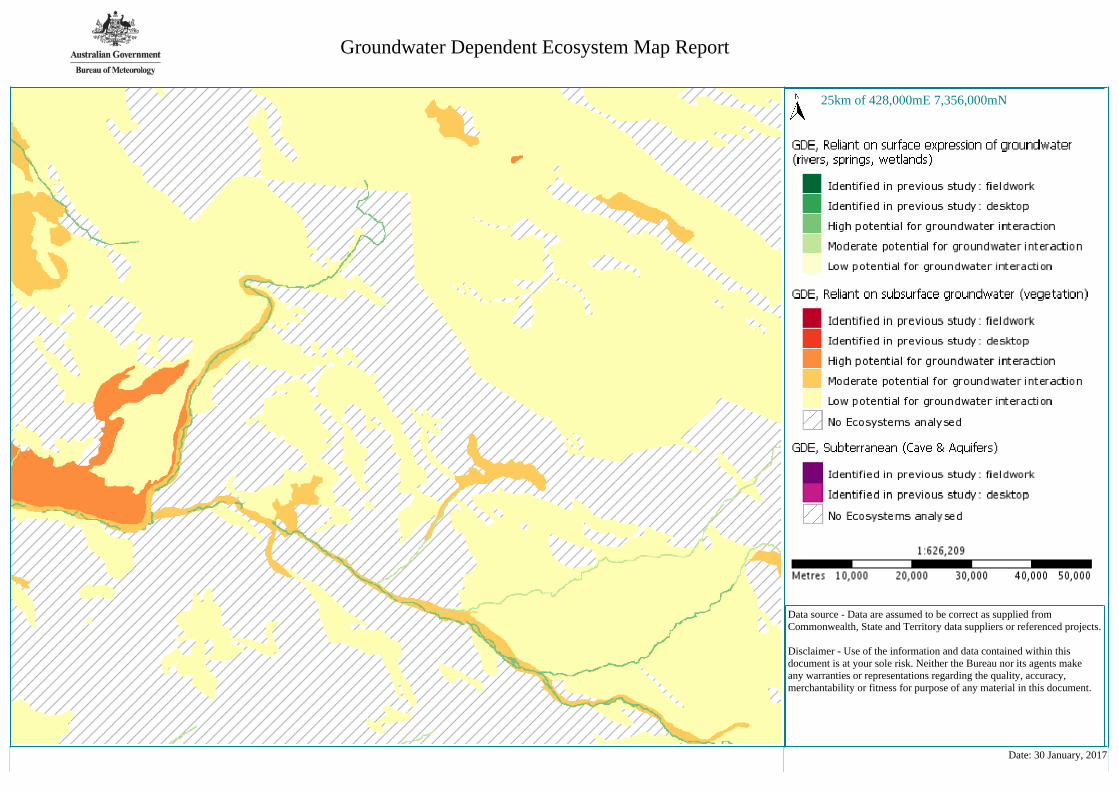
Groundwater Dependent Ecosystem Map Report
25km of 428,000mE 7,356,000mN
Data source - Data are assumed to be correct as supplied from Commonwealth, State and Territory data suppliers or referenced projects. Disclaimer - Use of the information and data contained within this document is at your sole risk. Neither the Bureau nor its agents make any warranties or representations regarding the quality, accuracy, merchantability or fitness for purpose of any material in this document.
Date: 30 January, 2017
J160014R01-Draft B-1 February 2017
APPENDIX B
Licence to Construct or Alter a Well
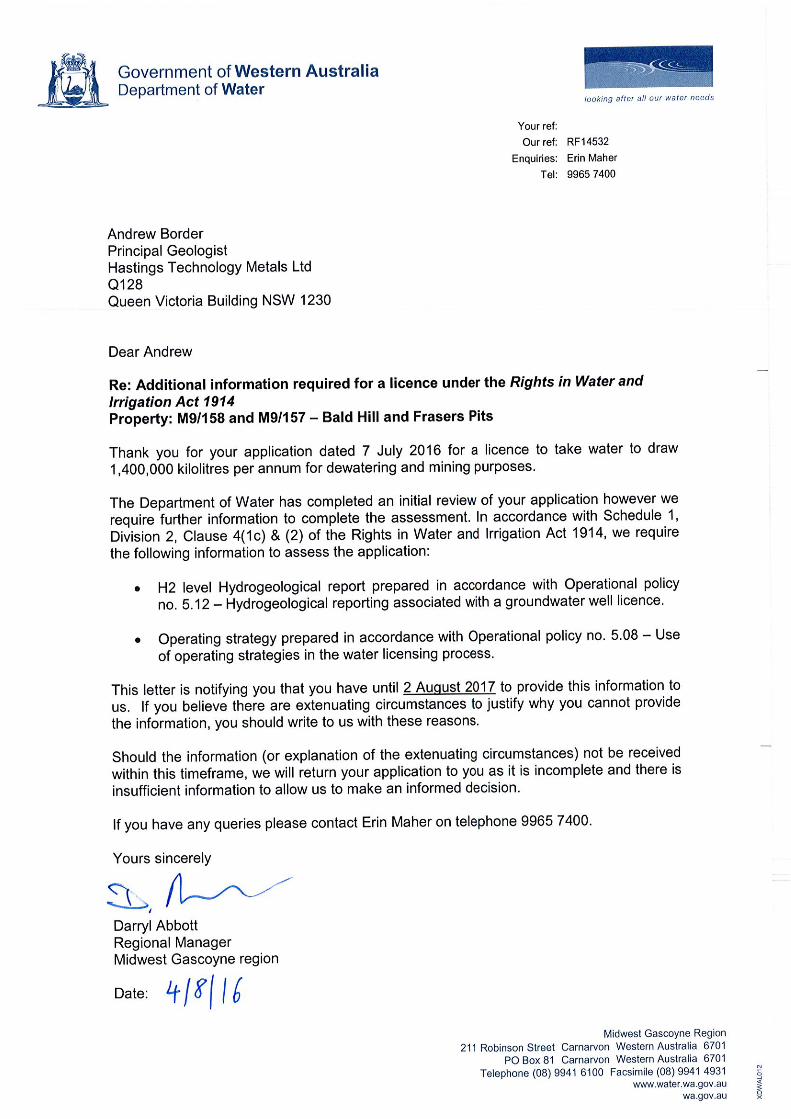
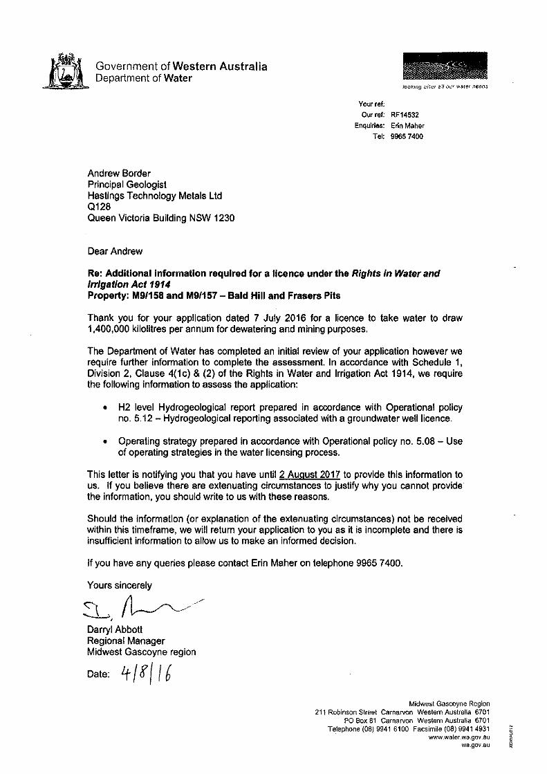

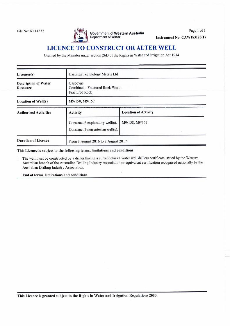

J160014R01 C-1 February 2017
APPENDIX C
Bore Logs
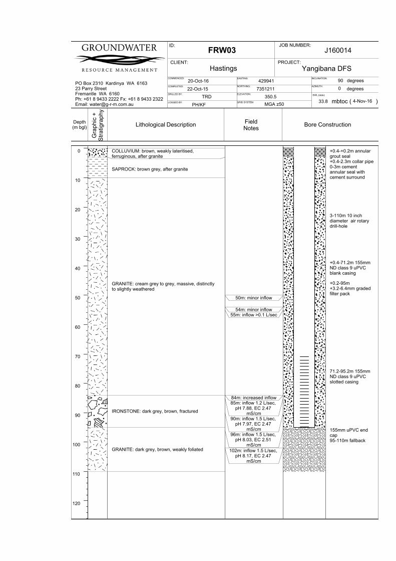
120
110
100
90
80
70
60
50
40
30
20
10
0 COLLUVIUM: brown, weakly lateritised,ferruginous, after granite
SAPROCK: brown grey, after granite
GRANITE: cream grey to grey, massive, distinctlyto slightly weathered
IRONSTONE: dark grey, brown, fractured
GRANITE: dark grey, brown, weakly foliated
50m: minor inflow
54m: minor inflow55m: inflow >0.1 L/sec
84m: increased inflow85m: inflow 1.2 L/sec,
pH 7.88, EC 2.47mS/cm
90m: inflow 1.5 L/sec,pH 7.97, EC 2.47
mS/cm96m: inflow 1.5 L/sec,
pH 8.03, EC 2.51mS/cm
102m: inflow 1.5 L/sec,pH 8.17, EC 2.47
mS/cm
+0.4-+0.2m annulargrout seal+0.4-2.3m collar pipe0-3m cementannular seal withcement surround
3-110m 10 inchdiameter air rotarydrill-hole
+0.4-71.2m 155mmND class 9 uPVCblank casing
+0.2-95m+3.2-6.4mm gradedfilter pack
71.2-95.2m 155mmND class 9 uPVCslotted casing
155mm uPVC endcap95-110m fallback
PO Box 2310 Kardinya WA 616323 Parry StreetFremantle WA 6160Ph: +61 8 9433 2222 Fx: +61 8 9433 2322Email: [email protected]
Depth(m bgl)
Gra
phic
+S
trat
igra
phy
Lithological Description FieldNotes
Bore Construction
ID: JOB NUMBER:
CLIENT: PROJECT:
COMMENCED:
COMPLETED:
DRILLED BY:
LOGGED BY:
INCLINATION:
AZIMUTH:
EASTING:
NORTHING:
ELEVATION:
GRID SYSTEM:
FRW03 J160014
Hastings Yangibana DFS
22-Oct-15
TRD
PH/KF
SWL (date):
7351211
350.5
MGA z50
90 degrees
degrees0
mbtoc ( )
42994120-Oct-16
4-Nov-1633.8

120
110
100
90
80
70
60
50
40
30
20
10
0 COLLUVIUM: brown, weakly lateritised,ferruginous, after granite
SAPROCK: brown grey, after granite
GRANITE: cream grey to grey, massive, distinctlyto slightly weathered, fractures 27-30m; 33-36m;and 41-45m
GRANITE: grey, massive, fresh to slightlyweathered
IRONSTONE: dark grey, brown, fractured
GRANITE: dark grey, brown, weakly foliated
36m: minor inflow38m: inflow <0.1 L/sec
42m: inflow <0.1 L/sec
48m: inflow 0.2 L/sec
55m: inflow 0.2 L/sec
63m: inflow 0.1 L/sec
68m: inflow 0.8 L/sec
76m: inflow 1 L/sec78m: inflow 1.2 L/sec
81m: inflow 2.9 L/sec83m: inflow 1.8 L/sec84m: inflow 2.2 L/sec
+0.4-+0.2m annulargrout seal+0.4-2.3m collar pipe0-3m cementannular seal withcement surround
3-110m 10 inchdiameter air rotarydrill-hole
+0.4-80m 155mmND class 9 uPVCblank casing
+0.2-104m+3.2-6.4mm gradedfilter pack
80-104m 155mmND class 9 uPVCslotted casing
155mm uPVC endcap104-110m fallback
PO Box 2310 Kardinya WA 616323 Parry StreetFremantle WA 6160Ph: +61 8 9433 2222 Fx: +61 8 9433 2322Email: [email protected]
Depth(m bgl)
Gra
phic
+S
trat
igra
phy
Lithological Description FieldNotes
Bore Construction
ID: JOB NUMBER:
CLIENT: PROJECT:
COMMENCED:
COMPLETED:
DRILLED BY:
LOGGED BY:
INCLINATION:
AZIMUTH:
EASTING:
NORTHING:
ELEVATION:
GRID SYSTEM:
BHW05 J160014
Hastings Yangibana DFS
13-Nov-16
TRD
PH/KF
SWL (date):
7356019
346.7
MGA z50
90 degrees
degrees0
mbtoc ( )
42818911-Nov-16

J160014R01 D-1 February 2017
APPENDIX D
Test Analysis
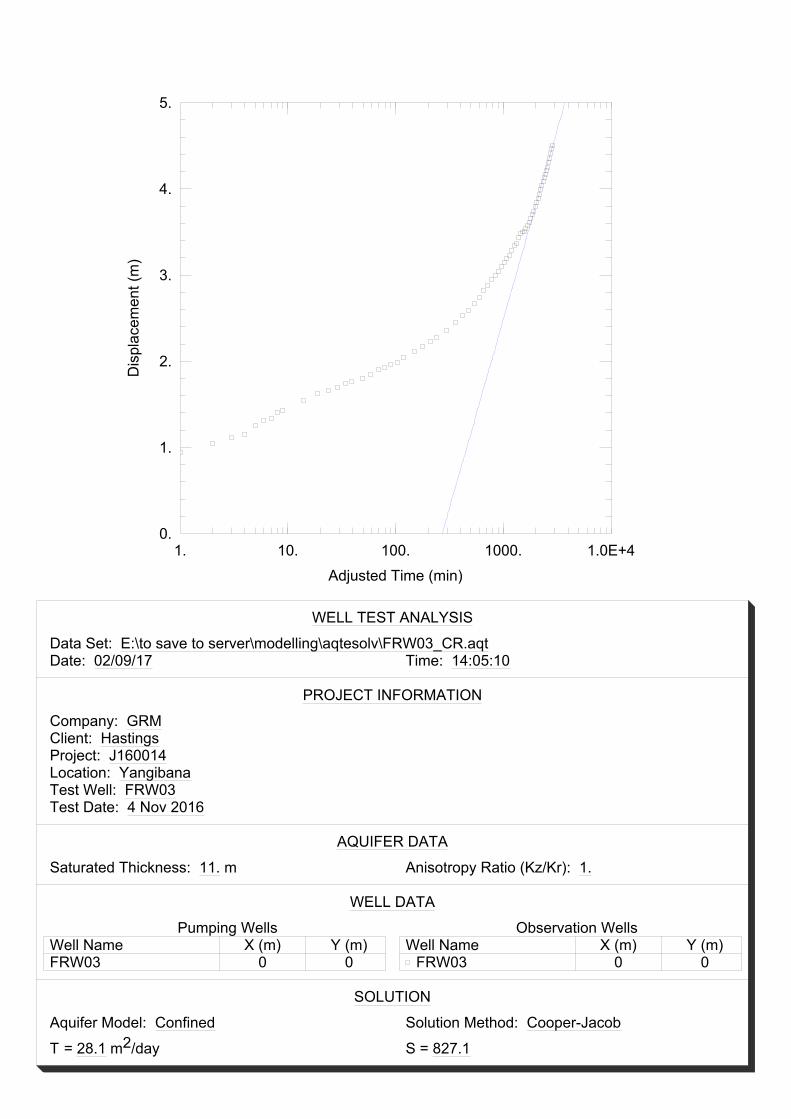
1. 10. 100. 1000. 1.0E+40.
1.
2.
3.
4.
5.
Adjusted Time (min)
Dis
plac
emen
t (m
)
WELL TEST ANALYSIS
Data Set: E:\to save to server\modelling\aqtesolv\FRW03_CR.aqtDate: 02/09/17 Time: 14:05:10
PROJECT INFORMATION
Company: GRMClient: HastingsProject: J160014Location: YangibanaTest Well: FRW03Test Date: 4 Nov 2016
AQUIFER DATA
Saturated Thickness: 11. m Anisotropy Ratio (Kz/Kr): 1.
WELL DATA
Pumping WellsWell Name X (m) Y (m)FRW03 0 0
Observation WellsWell Name X (m) Y (m)
FRW03 0 0
SOLUTION
Aquifer Model: Confined Solution Method: Cooper-Jacob
T = 28.1 m2/day S = 827.1

1. 10. 100. 1000. 1.0E+40.
1.
2.
3.
4.
5.
Time, t/t'
Res
idua
l Dra
wdo
wn
(m)
WELL TEST ANALYSIS
Data Set: E:\to save to server\modelling\aqtesolv\FRW03_recET.aqtDate: 02/09/17 Time: 14:07:30
PROJECT INFORMATION
Company: GRMClient: HastingsProject: J160014Location: YangibanaTest Well: FRW03Test Date: 6 Nov 2016
AQUIFER DATA
Saturated Thickness: 11. m Anisotropy Ratio (Kz/Kr): 1.
WELL DATA
Pumping WellsWell Name X (m) Y (m)FRW03 0 0
Observation WellsWell Name X (m) Y (m)
FRW03 0 0
SOLUTION
Aquifer Model: Confined Solution Method: Theis (Recovery)
T = 329.4 m2/day S/S' = 1.66E-9

1. 10. 100. 1000. 1.0E+40.
1.
2.
3.
4.
5.
Time, t/t'
Res
idua
l Dra
wdo
wn
(m)
WELL TEST ANALYSIS
Data Set: E:\to save to server\modelling\aqtesolv\FRW03_recLT.aqtDate: 02/09/17 Time: 14:09:08
PROJECT INFORMATION
Company: GRMClient: HastingsProject: J160014Location: YangibanaTest Well: FRW03Test Date: 6 Nov 2016
AQUIFER DATA
Saturated Thickness: 11. m Anisotropy Ratio (Kz/Kr): 1.
WELL DATA
Pumping WellsWell Name X (m) Y (m)FRW03 0 0
Observation WellsWell Name X (m) Y (m)
FRW03 0 0
SOLUTION
Aquifer Model: Confined Solution Method: Theis (Recovery)
T = 197.6 m2/day S/S' = 3.162E-5

1. 10. 100. 1000. 1.0E+40.
0.8
1.6
2.4
3.2
4.
Adjusted Time (min)
Dis
plac
emen
t (m
)
WELL TEST ANALYSIS
Data Set: E:\to save to server\modelling\aqtesolv\FRW01obs_CR.aqtDate: 02/09/17 Time: 14:10:34
PROJECT INFORMATION
Company: GRMClient: HastingsProject: J160014Location: YangibanaTest Well: FRW03Test Date: 4 Nov 2016
AQUIFER DATA
Saturated Thickness: 11. m Anisotropy Ratio (Kz/Kr): 1.
WELL DATA
Pumping WellsWell Name X (m) Y (m)FRW03 0 0
Observation WellsWell Name X (m) Y (m)
FRW01 6 0
SOLUTION
Aquifer Model: Confined Solution Method: Cooper-Jacob
T = 28.37 m2/day S = 0.4489
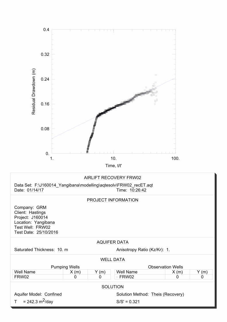
1. 10. 100.0.
0.08
0.16
0.24
0.32
0.4
Time, t/t'
Res
idua
l Dra
wdo
wn
(m)
AIRLIFT RECOVERY FRW02
Data Set: F:\J160014_Yangibana\modelling\aqtesolv\FRW02_recET.aqtDate: 01/14/17 Time: 10:26:42
PROJECT INFORMATION
Company: GRMClient: HastingsProject: J160014Location: YangibanaTest Well: FRW02Test Date: 25/10/2016
AQUIFER DATA
Saturated Thickness: 10. m Anisotropy Ratio (Kz/Kr): 1.
WELL DATA
Pumping WellsWell Name X (m) Y (m)FRW02 0 0
Observation WellsWell Name X (m) Y (m)
FRW02 0 0
SOLUTION
Aquifer Model: Confined Solution Method: Theis (Recovery)
T = 242.3 m2/day S/S' = 0.321
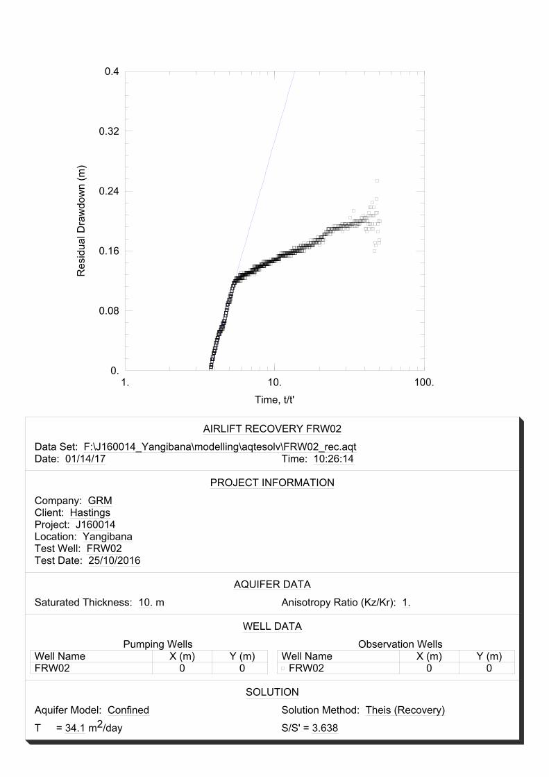
1. 10. 100.0.
0.08
0.16
0.24
0.32
0.4
Time, t/t'
Res
idua
l Dra
wdo
wn
(m)
AIRLIFT RECOVERY FRW02
Data Set: F:\J160014_Yangibana\modelling\aqtesolv\FRW02_rec.aqtDate: 01/14/17 Time: 10:26:14
PROJECT INFORMATION
Company: GRMClient: HastingsProject: J160014Location: YangibanaTest Well: FRW02Test Date: 25/10/2016
AQUIFER DATA
Saturated Thickness: 10. m Anisotropy Ratio (Kz/Kr): 1.
WELL DATA
Pumping WellsWell Name X (m) Y (m)FRW02 0 0
Observation WellsWell Name X (m) Y (m)
FRW02 0 0
SOLUTION
Aquifer Model: Confined Solution Method: Theis (Recovery)
T = 34.1 m2/day S/S' = 3.638

1. 10. 100. 1000. 1.0E+40.
0.1
0.2
0.3
0.4
0.5
Time, t/t'
Res
idua
l Dra
wdo
wn
(m)
AIRLIFT RECOVERY FFRC082
Data Set: F:\J160014_Yangibana\modelling\aqtesolv\FRC082_rec_logger.aqtDate: 01/06/17 Time: 15:39:04
PROJECT INFORMATION
Company: GRMClient: HastingsProject: J160014Location: YangibanaTest Well: FFRC082Test Date: 26/10/2016
AQUIFER DATA
Saturated Thickness: 6. m Anisotropy Ratio (Kz/Kr): 1.
WELL DATA
Pumping WellsWell Name X (m) Y (m)FFRC082 0 0
Observation WellsWell Name X (m) Y (m)
FFRC082 0 0
SOLUTION
Aquifer Model: Confined Solution Method: Theis (Recovery)
T = 226.6 m2/day S/S' = 2.057

1. 10. 100.6.
8.
10.
12.
14.
16.
Time, t/t'
Res
idua
l Dra
wdo
wn
(m)
AIRLIFT RECOVERY FFRC098
Data Set: F:\J160014_Yangibana\modelling\aqtesolv\FRC098_rec_logger.aqtDate: 01/14/17 Time: 12:32:36
PROJECT INFORMATION
Company: GRMClient: HastingsProject: J160014Location: YangibanaTest Well: FFRC082Test Date: 26/10/2016
AQUIFER DATA
Saturated Thickness: 14.9 m Anisotropy Ratio (Kz/Kr): 1.
WELL DATA
Pumping WellsWell Name X (m) Y (m)FFRC098 0 0
Observation WellsWell Name X (m) Y (m)
FFRC098 0 0
SOLUTION
Aquifer Model: Confined Solution Method: Theis (Recovery)
T = 0.1156 m2/day S/S' = 6.315E-5

1. 10. 100.6.
8.
10.
12.
14.
16.
Time, t/t'
Res
idua
l Dra
wdo
wn
(m)
AIRLIFT RECOVERY FFRC098
Data Set: F:\J160014_Yangibana\modelling\aqtesolv\FRC098_rec_loggerLT.aqtDate: 01/14/17 Time: 12:32:12
PROJECT INFORMATION
Company: GRMClient: HastingsProject: J160014Location: YangibanaTest Well: FFRC082Test Date: 26/10/2016
AQUIFER DATA
Saturated Thickness: 14.9 m Anisotropy Ratio (Kz/Kr): 1.
WELL DATA
Pumping WellsWell Name X (m) Y (m)FFRC098 0 0
Observation WellsWell Name X (m) Y (m)
FFRC098 0 0
SOLUTION
Aquifer Model: Confined Solution Method: Theis (Recovery)
T = 0.02527 m2/day S/S' = 1.06

1. 10. 100. 1000. 1.0E+40.
3.2
6.4
9.6
12.8
16.
Adjusted Time (min)
Dis
plac
emen
t (m
)
WELL TEST ANALYSIS
Data Set: F:\J160014_Yangibana\modelling\aqtesolv\BHW05_CR.aqtDate: 01/14/17 Time: 14:15:52
PROJECT INFORMATION
Company: GRMClient: HastingsProject: J160014Location: YangibanaTest Well: BHW05Test Date: 9 Dec 2016
AQUIFER DATA
Saturated Thickness: 20. m Anisotropy Ratio (Kz/Kr): 1.
WELL DATA
Pumping WellsWell Name X (m) Y (m)BHW05 0 0
Observation WellsWell Name X (m) Y (m)
BHW05 0 0
SOLUTION
Aquifer Model: Confined Solution Method: Cooper-Jacob
T = 236.1 m2/day S = 0.0001196
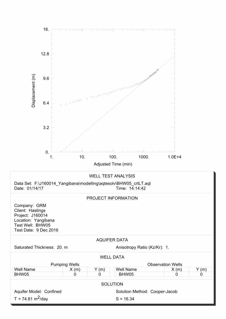
1. 10. 100. 1000. 1.0E+40.
3.2
6.4
9.6
12.8
16.
Adjusted Time (min)
Dis
plac
emen
t (m
)
WELL TEST ANALYSIS
Data Set: F:\J160014_Yangibana\modelling\aqtesolv\BHW05_crtLT.aqtDate: 01/14/17 Time: 14:14:42
PROJECT INFORMATION
Company: GRMClient: HastingsProject: J160014Location: YangibanaTest Well: BHW05Test Date: 9 Dec 2016
AQUIFER DATA
Saturated Thickness: 20. m Anisotropy Ratio (Kz/Kr): 1.
WELL DATA
Pumping WellsWell Name X (m) Y (m)BHW05 0 0
Observation WellsWell Name X (m) Y (m)
BHW05 0 0
SOLUTION
Aquifer Model: Confined Solution Method: Cooper-Jacob
T = 74.81 m2/day S = 16.34

1. 10. 100. 1000. 1.0E+40.
1.2
2.4
3.6
4.8
6.
Time, t/t'
Res
idua
l Dra
wdo
wn
(m)
WELL TEST ANALYSIS
Data Set: F:\J160014_Yangibana\modelling\aqtesolv\BHW05_recET.aqtDate: 01/14/17 Time: 14:32:01
PROJECT INFORMATION
Company: GRMClient: HastingsProject: J160014Location: YangibanaTest Well: BHW05Test Date: 11 Dec 2016
AQUIFER DATA
Saturated Thickness: 20. m Anisotropy Ratio (Kz/Kr): 1.
WELL DATA
Pumping WellsWell Name X (m) Y (m)BHW05 0 0
Observation WellsWell Name X (m) Y (m)
BHW05 0 0
SOLUTION
Aquifer Model: Confined Solution Method: Theis (Recovery)
T = 207. m2/day S/S' = 0.1134

1. 10. 100. 1000. 1.0E+40.
1.2
2.4
3.6
4.8
6.
Time, t/t'
Res
idua
l Dra
wdo
wn
(m)
WELL TEST ANALYSIS
Data Set: F:\J160014_Yangibana\modelling\aqtesolv\BHW05_recLT.aqtDate: 01/14/17 Time: 14:31:26
PROJECT INFORMATION
Company: GRMClient: HastingsProject: J160014Location: YangibanaTest Well: BHW05Test Date: 11 Dec 2016
AQUIFER DATA
Saturated Thickness: 20. m Anisotropy Ratio (Kz/Kr): 1.
WELL DATA
Pumping WellsWell Name X (m) Y (m)BHW05 0 0
Observation WellsWell Name X (m) Y (m)
BHW05 0 0
SOLUTION
Aquifer Model: Confined Solution Method: Theis (Recovery)
T = 216.5 m2/day S/S' = 0.05542

1. 10. 100. 1000. 1.0E+40.
1.6
3.2
4.8
6.4
8.
Adjusted Time (min)
Dis
plac
emen
t (m
)
WELL TEST ANALYSIS
Data Set: F:\J160014_Yangibana\modelling\aqtesolv\BHW05obs_crtET.aqtDate: 01/14/17 Time: 15:06:24
PROJECT INFORMATION
Company: GRMClient: HastingsProject: J160014Location: YangibanaTest Well: BHW05Test Date: 9 Dec 2016
AQUIFER DATA
Saturated Thickness: 20. m Anisotropy Ratio (Kz/Kr): 1.
WELL DATA
Pumping WellsWell Name X (m) Y (m)BHW05 0 0
Observation WellsWell Name X (m) Y (m)
BHW05obs 7.4 0
SOLUTION
Aquifer Model: Confined Solution Method: Cooper-Jacob
T = 223.8 m2/day S = 0.0004285

1. 10. 100. 1000. 1.0E+40.
1.6
3.2
4.8
6.4
8.
Adjusted Time (min)
Dis
plac
emen
t (m
)
WELL TEST ANALYSIS
Data Set: F:\J160014_Yangibana\modelling\aqtesolv\BHW05obs_crtLT.aqtDate: 01/14/17 Time: 15:06:05
PROJECT INFORMATION
Company: GRMClient: HastingsProject: J160014Location: YangibanaTest Well: BHW05Test Date: 9 Dec 2016
AQUIFER DATA
Saturated Thickness: 20. m Anisotropy Ratio (Kz/Kr): 1.
WELL DATA
Pumping WellsWell Name X (m) Y (m)BHW05 0 0
Observation WellsWell Name X (m) Y (m)
BHW05obs 7.4 0
SOLUTION
Aquifer Model: Confined Solution Method: Cooper-Jacob
T = 68.36 m2/day S = 0.09607

1. 10. 100. 1000. 1.0E+40.
1.2
2.4
3.6
4.8
6.
Time, t/t'
Res
idua
l Dra
wdo
wn
(m)
WELL TEST ANALYSIS
Data Set: F:\J160014_Yangibana\modelling\aqtesolv\BHW05_obs recLT.aqtDate: 01/14/17 Time: 14:50:55
PROJECT INFORMATION
Company: GRMClient: HastingsProject: J160014Location: YangibanaTest Well: BHW05obsTest Date: 11 Dec 2016
AQUIFER DATA
Saturated Thickness: 20. m Anisotropy Ratio (Kz/Kr): 1.
WELL DATA
Pumping WellsWell Name X (m) Y (m)BHW05obs 7.4 0
Observation WellsWell Name X (m) Y (m)
BHW05obs 7.4 0
SOLUTION
Aquifer Model: Confined Solution Method: Theis (Recovery)
T = 231.9 m2/day S/S' = 0.0347
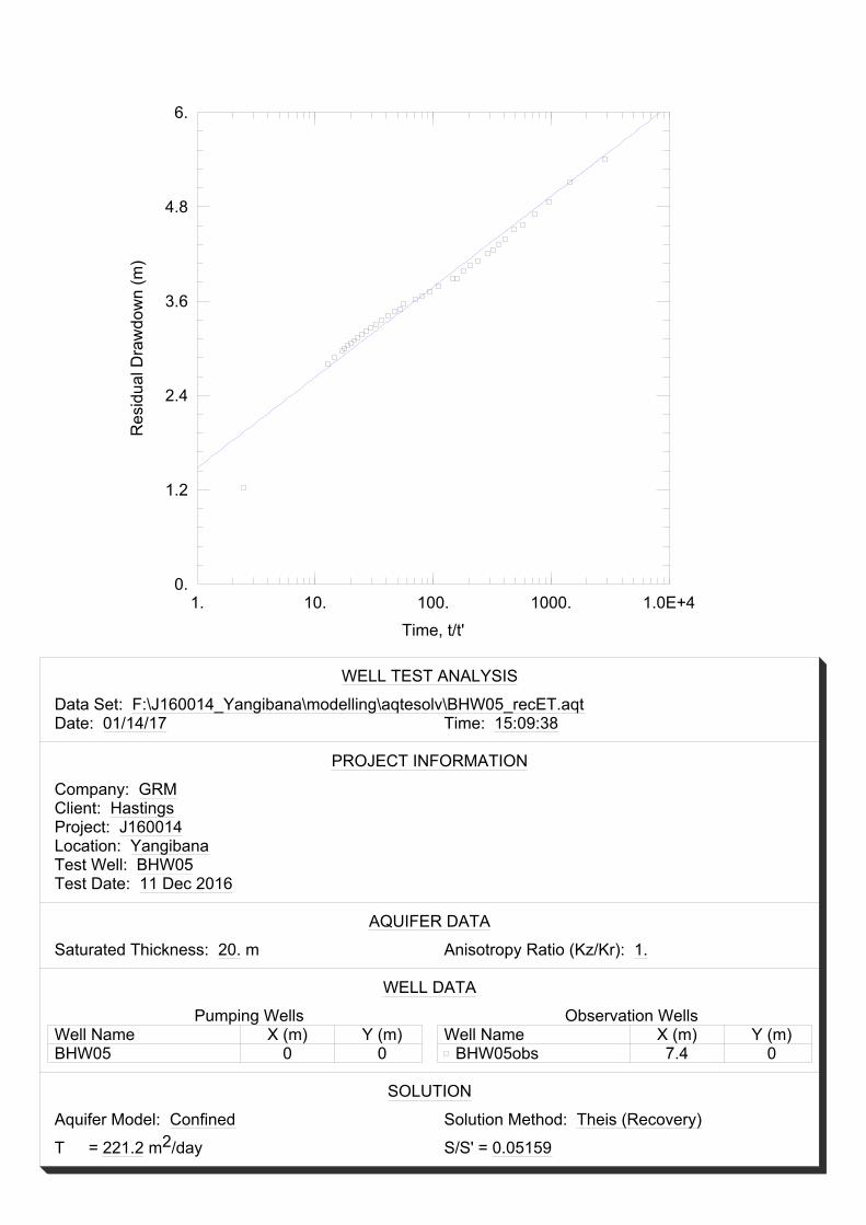
1. 10. 100. 1000. 1.0E+40.
1.2
2.4
3.6
4.8
6.
Time, t/t'
Res
idua
l Dra
wdo
wn
(m)
WELL TEST ANALYSIS
Data Set: F:\J160014_Yangibana\modelling\aqtesolv\BHW05_recET.aqtDate: 01/14/17 Time: 15:09:38
PROJECT INFORMATION
Company: GRMClient: HastingsProject: J160014Location: YangibanaTest Well: BHW05Test Date: 11 Dec 2016
AQUIFER DATA
Saturated Thickness: 20. m Anisotropy Ratio (Kz/Kr): 1.
WELL DATA
Pumping WellsWell Name X (m) Y (m)BHW05 0 0
Observation WellsWell Name X (m) Y (m)
BHW05obs 7.4 0
SOLUTION
Aquifer Model: Confined Solution Method: Theis (Recovery)
T = 221.2 m2/day S/S' = 0.05159

1. 10. 100.0.
0.32
0.64
0.96
1.28
1.6
Time, t/t'
Res
idua
l Dra
wdo
wn
(m)
AIRLIFT RECOVERY BHW01
Data Set: F:\J160014_Yangibana\modelling\aqtesolv\BHW01.aqtDate: 01/14/17 Time: 15:48:09
PROJECT INFORMATION
Company: GRMClient: HastingsProject: J160014Location: YangibanaTest Well: BHW01Test Date: 18/11/2016
AQUIFER DATA
Saturated Thickness: 20. m Anisotropy Ratio (Kz/Kr): 1.
WELL DATA
Pumping WellsWell Name X (m) Y (m)BHW01 0 0
Observation WellsWell Name X (m) Y (m)
BHW01 0 0
SOLUTION
Aquifer Model: Confined Solution Method: Theis (Recovery)
T = 100. m2/day S/S' = 0.7462
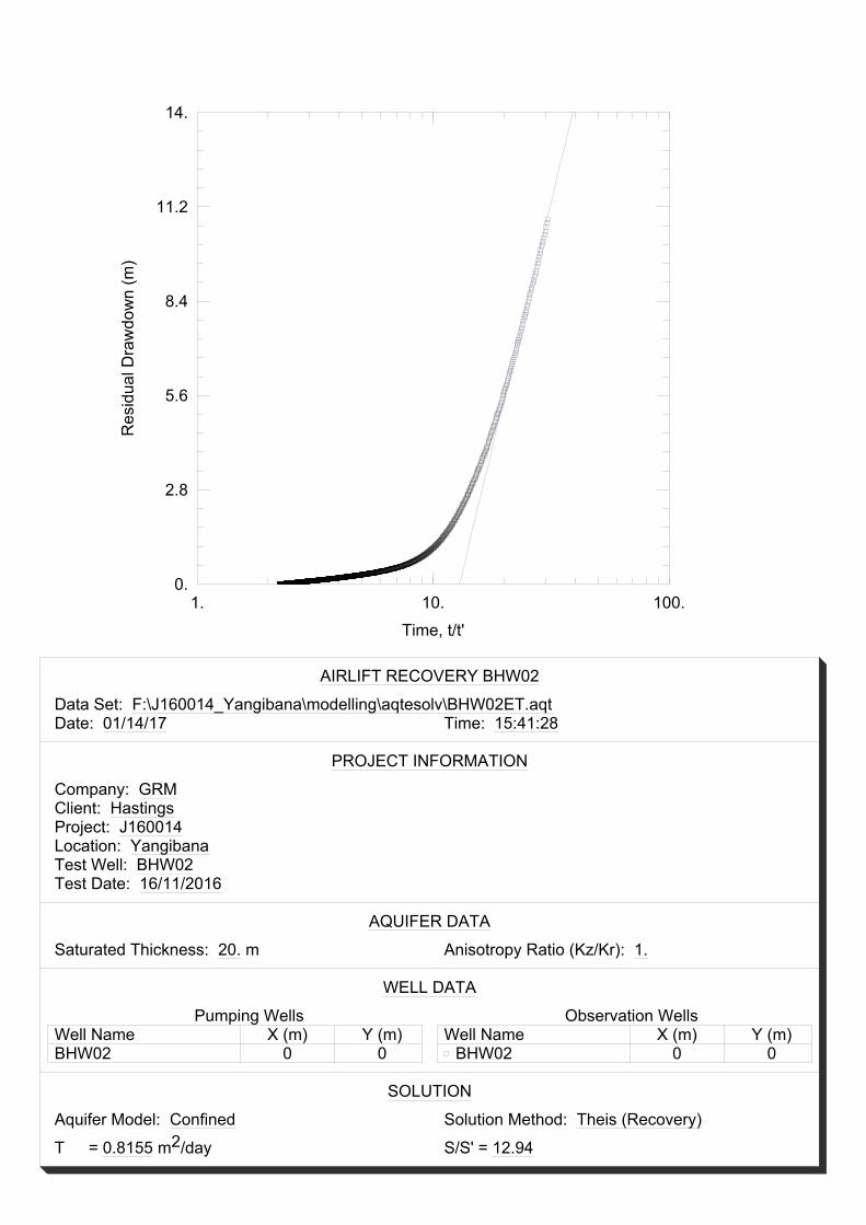
1. 10. 100.0.
2.8
5.6
8.4
11.2
14.
Time, t/t'
Res
idua
l Dra
wdo
wn
(m)
AIRLIFT RECOVERY BHW02
Data Set: F:\J160014_Yangibana\modelling\aqtesolv\BHW02ET.aqtDate: 01/14/17 Time: 15:41:28
PROJECT INFORMATION
Company: GRMClient: HastingsProject: J160014Location: YangibanaTest Well: BHW02Test Date: 16/11/2016
AQUIFER DATA
Saturated Thickness: 20. m Anisotropy Ratio (Kz/Kr): 1.
WELL DATA
Pumping WellsWell Name X (m) Y (m)BHW02 0 0
Observation WellsWell Name X (m) Y (m)
BHW02 0 0
SOLUTION
Aquifer Model: Confined Solution Method: Theis (Recovery)
T = 0.8155 m2/day S/S' = 12.94

1. 10. 100.0.
2.8
5.6
8.4
11.2
14.
Time, t/t'
Res
idua
l Dra
wdo
wn
(m)
AIRLIFT RECOVERY BHW02
Data Set: F:\J160014_Yangibana\modelling\aqtesolv\BHW02.aqtDate: 01/07/17 Time: 15:11:04
PROJECT INFORMATION
Company: GRMClient: HastingsProject: J160014Location: YangibanaTest Well: BHW02Test Date: 16/11/2016
AQUIFER DATA
Saturated Thickness: 20. m Anisotropy Ratio (Kz/Kr): 1.
WELL DATA
Pumping WellsWell Name X (m) Y (m)BHW02 0 0
Observation WellsWell Name X (m) Y (m)
BHW02 0 0
SOLUTION
Aquifer Model: Confined Solution Method: Theis (Recovery)
T = 31.58 m2/day S/S' = 1.999

1. 10. 100.0.
0.8
1.6
2.4
3.2
4.
Time, t/t'
Res
idua
l Dra
wdo
wn
(m)
AIRLIFT RECOVERY BHRC161
Data Set: F:\J160014_Yangibana\modelling\aqtesolv\BHRC161 early.aqtDate: 01/14/17 Time: 15:55:21
PROJECT INFORMATION
Company: GRMClient: HastingsProject: J160014Location: YangibanaTest Well: BHRC161Test Date: 20/11/2016
AQUIFER DATA
Saturated Thickness: 5. m Anisotropy Ratio (Kz/Kr): 1.
WELL DATA
Pumping WellsWell Name X (m) Y (m)BHRC161 0 0
Observation WellsWell Name X (m) Y (m)
BHRC161 0 0
SOLUTION
Aquifer Model: Confined Solution Method: Theis (Recovery)
T = 16.99 m2/day S/S' = 10.51

1. 10. 100.0.
0.8
1.6
2.4
3.2
4.
Time, t/t'
Res
idua
l Dra
wdo
wn
(m)
AIRLIFT RECOVERY BHRC161
Data Set: F:\J160014_Yangibana\modelling\aqtesolv\BHRC161.aqtDate: 01/06/17 Time: 16:26:26
PROJECT INFORMATION
Company: GRMClient: HastingsProject: J160014Location: YangibanaTest Well: BHRC161Test Date: 20/11/2016
AQUIFER DATA
Saturated Thickness: 5. m Anisotropy Ratio (Kz/Kr): 1.
WELL DATA
Pumping WellsWell Name X (m) Y (m)BHRC161 0 0
Observation WellsWell Name X (m) Y (m)
BHRC161 0 0
SOLUTION
Aquifer Model: Confined Solution Method: Theis (Recovery)
T = 79.91 m2/day S/S' = 1.117

1. 10. 100. 1000.0.
0.2
0.4
0.6
0.8
1.
Time, t/t'
Res
idua
l Dra
wdo
wn
(m)
AIRLIFT RECOVERY BHRC082
Data Set: F:\J160014_Yangibana\modelling\aqtesolv\BHRC082.aqtDate: 01/14/17 Time: 16:01:00
PROJECT INFORMATION
Company: GRMClient: HastingsProject: J160014Location: YangibanaTest Well: BHRC082Test Date: 20/11/2016
AQUIFER DATA
Saturated Thickness: 34.77 m Anisotropy Ratio (Kz/Kr): 1.
WELL DATA
Pumping WellsWell Name X (m) Y (m)BHRC082 0 0
Observation WellsWell Name X (m) Y (m)
BHRC082 0 0
SOLUTION
Aquifer Model: Confined Solution Method: Theis (Recovery)
T = 66.01 m2/day S/S' = 1.505
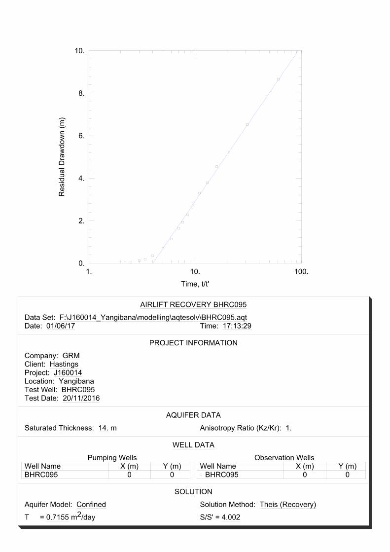
1. 10. 100.0.
2.
4.
6.
8.
10.
Time, t/t'
Res
idua
l Dra
wdo
wn
(m)
AIRLIFT RECOVERY BHRC095
Data Set: F:\J160014_Yangibana\modelling\aqtesolv\BHRC095.aqtDate: 01/06/17 Time: 17:13:29
PROJECT INFORMATION
Company: GRMClient: HastingsProject: J160014Location: YangibanaTest Well: BHRC095Test Date: 20/11/2016
AQUIFER DATA
Saturated Thickness: 14. m Anisotropy Ratio (Kz/Kr): 1.
WELL DATA
Pumping WellsWell Name X (m) Y (m)BHRC095 0 0
Observation WellsWell Name X (m) Y (m)
BHRC095 0 0
SOLUTION
Aquifer Model: Confined Solution Method: Theis (Recovery)
T = 0.7155 m2/day S/S' = 4.002

0. 100. 200. 300. 400. 500.0.001
0.01
0.1
1.
Time (sec)
Dis
plac
emen
t (m
)
WELL TEST ANALYSIS
Data Set: F:\J160014_Yangibana\modelling\aqtesolv\Daves\BHRC097.aqtDate: 01/14/17 Time: 16:14:46
PROJECT INFORMATION
Company: GRMClient: HastingsProject: J160014Location: YangibanaTest Well: BHRC097Test Date: 18 Dec 2016
AQUIFER DATA
Saturated Thickness: 40.48 m Anisotropy Ratio (Kz/Kr): 1.
WELL DATA (BHRC097)
Initial Displacement: 0.1628 m Static Water Column Height: 40.48 mTotal Well Penetration Depth: 40.48 m Screen Length: 40.48 mCasing Radius: 0.075 m Well Radius: 0.075 m
Gravel Pack Porosity: 1.
SOLUTION
Aquifer Model: Unconfined Solution Method: Hvorslev
K = 0.25 m/day y0 = 0.1635 m

1. 10. 100. 1000. 1.0E+40.
2.4
4.8
7.2
9.6
12.
Adjusted Time (min)
Dis
plac
emen
t (m
)
WELL TEST ANALYSIS
Data Set: F:\J160014_Yangibana\modelling\aqtesolv\Daves\YGWB003.aqtDate: 01/14/17 Time: 20:24:01
PROJECT INFORMATION
Company: GRMClient: HastingsProject: J160014Location: YangibanaTest Well: YGWB003Test Date: 14 Dec 2016
AQUIFER DATA
Saturated Thickness: 10. m Anisotropy Ratio (Kz/Kr): 1.
WELL DATA
Pumping WellsWell Name X (m) Y (m)YGWB003 0 0
Observation WellsWell Name X (m) Y (m)
YGWB003 0 0
SOLUTION
Aquifer Model: Confined Solution Method: Cooper-Jacob
T = 54.95 m2/day S = 1.008E-6

1. 10. 100. 1000. 1.0E+40.
0.8
1.6
2.4
3.2
4.
Time, t/t'
Res
idua
l Dra
wdo
wn
(m)
WELL TEST ANALYSIS
Data Set: F:\J160014_Yangibana\modelling\aqtesolv\YGWB003recET.aqtDate: 01/15/17 Time: 14:42:30
PROJECT INFORMATION
Company: GRMClient: HastingsProject: J160014Location: YangibanaTest Well: YGWB003Test Date: 16 Dec 2016
AQUIFER DATA
Saturated Thickness: 10. m Anisotropy Ratio (Kz/Kr): 1.
WELL DATA
Pumping WellsWell Name X (m) Y (m)YGWB003 0 0
Observation WellsWell Name X (m) Y (m)
YGWB003 0 0
SOLUTION
Aquifer Model: Confined Solution Method: Theis (Recovery)
T = 29.75 m2/day S/S' = 32.49

1. 10. 100. 1000. 1.0E+40.
0.8
1.6
2.4
3.2
4.
Time, t/t'
Res
idua
l Dra
wdo
wn
(m)
WELL TEST ANALYSIS
Data Set: F:\J160014_Yangibana\modelling\aqtesolv\YGWB003recLT.aqtDate: 01/15/17 Time: 14:42:57
PROJECT INFORMATION
Company: GRMClient: HastingsProject: J160014Location: YangibanaTest Well: YGWB003Test Date: 16 Dec 2016
AQUIFER DATA
Saturated Thickness: 10. m Anisotropy Ratio (Kz/Kr): 1.
WELL DATA
Pumping WellsWell Name X (m) Y (m)YGWB003 0 0
Observation WellsWell Name X (m) Y (m)
YGWB003 0 0
SOLUTION
Aquifer Model: Confined Solution Method: Theis (Recovery)
T = 82.61 m2/day S/S' = 0.0985
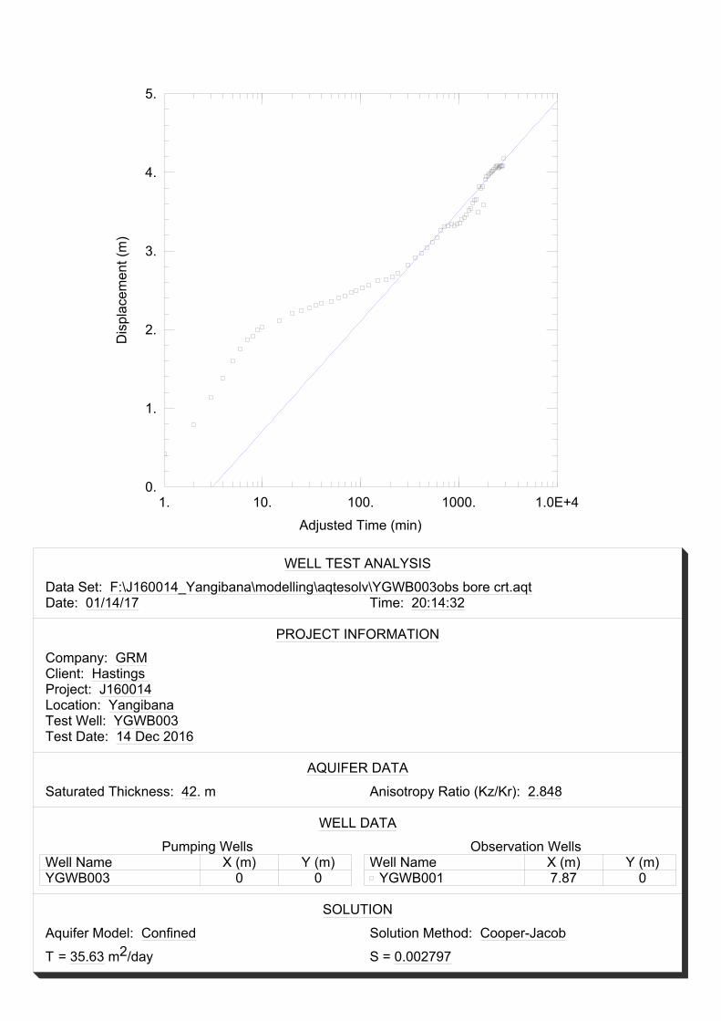
1. 10. 100. 1000. 1.0E+40.
1.
2.
3.
4.
5.
Adjusted Time (min)
Dis
plac
emen
t (m
)
WELL TEST ANALYSIS
Data Set: F:\J160014_Yangibana\modelling\aqtesolv\YGWB003obs bore crt.aqtDate: 01/14/17 Time: 20:14:32
PROJECT INFORMATION
Company: GRMClient: Hastings Project: J160014Location: YangibanaTest Well: YGWB003Test Date: 14 Dec 2016
AQUIFER DATA
Saturated Thickness: 42. m Anisotropy Ratio (Kz/Kr): 2.848
WELL DATA
Pumping WellsWell Name X (m) Y (m)YGWB003 0 0
Observation WellsWell Name X (m) Y (m)
YGWB001 7.87 0
SOLUTION
Aquifer Model: Confined Solution Method: Cooper-Jacob
T = 35.63 m2/day S = 0.002797
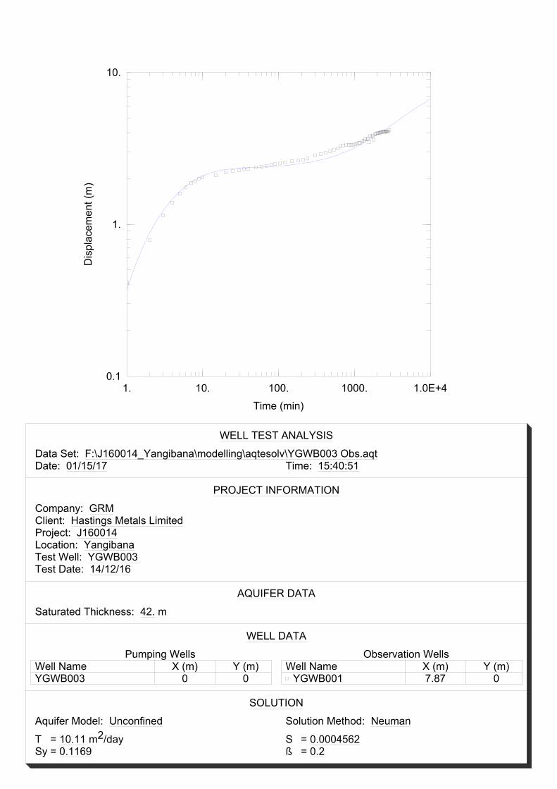
1. 10. 100. 1000. 1.0E+40.1
1.
10.
Time (min)
Dis
plac
emen
t (m
)
WELL TEST ANALYSIS
Data Set: F:\J160014_Yangibana\modelling\aqtesolv\YGWB003 Obs.aqtDate: 01/15/17 Time: 15:40:51
PROJECT INFORMATION
Company: GRMClient: Hastings Metals LimitedProject: J160014Location: YangibanaTest Well: YGWB003Test Date: 14/12/16
AQUIFER DATA
Saturated Thickness: 42. m
WELL DATA
Pumping WellsWell Name X (m) Y (m)YGWB003 0 0
Observation WellsWell Name X (m) Y (m)
YGWB001 7.87 0
SOLUTION
Aquifer Model: Unconfined Solution Method: Neuman
T = 10.11 m2/day S = 0.0004562Sy = 0.1169 ß = 0.2
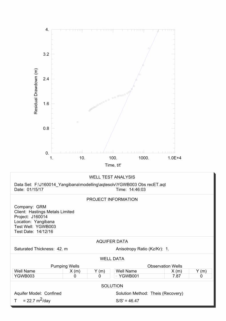
1. 10. 100. 1000. 1.0E+40.
0.8
1.6
2.4
3.2
4.
Time, t/t'
Res
idua
l Dra
wdo
wn
(m)
WELL TEST ANALYSIS
Data Set: F:\J160014_Yangibana\modelling\aqtesolv\YGWB003 Obs recET.aqtDate: 01/15/17 Time: 14:46:03
PROJECT INFORMATION
Company: GRMClient: Hastings Metals LimitedProject: J160014Location: YangibanaTest Well: YGWB003Test Date: 14/12/16
AQUIFER DATA
Saturated Thickness: 42. m Anisotropy Ratio (Kz/Kr): 1.
WELL DATA
Pumping WellsWell Name X (m) Y (m)YGWB003 0 0
Observation WellsWell Name X (m) Y (m)
YGWB001 7.87 0
SOLUTION
Aquifer Model: Confined Solution Method: Theis (Recovery)
T = 22.7 m2/day S/S' = 46.47
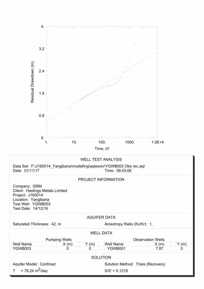
1. 10. 100. 1000. 1.0E+40.
0.8
1.6
2.4
3.2
4.
Time, t/t'
Res
idua
l Dra
wdo
wn
(m)
WELL TEST ANALYSIS
Data Set: F:\J160014_Yangibana\modelling\aqtesolv\YGWB003 Obs rec.aqtDate: 01/11/17 Time: 08:43:06
PROJECT INFORMATION
Company: GRMClient: Hastings Metals LimitedProject: J160014Location: YangibanaTest Well: YGWB003Test Date: 14/12/16
AQUIFER DATA
Saturated Thickness: 42. m Anisotropy Ratio (Kz/Kr): 1.
WELL DATA
Pumping WellsWell Name X (m) Y (m)YGWB003 0 0
Observation WellsWell Name X (m) Y (m)
YGWB001 7.87 0
SOLUTION
Aquifer Model: Confined Solution Method: Theis (Recovery)
T = 78.24 m2/day S/S' = 0.1218
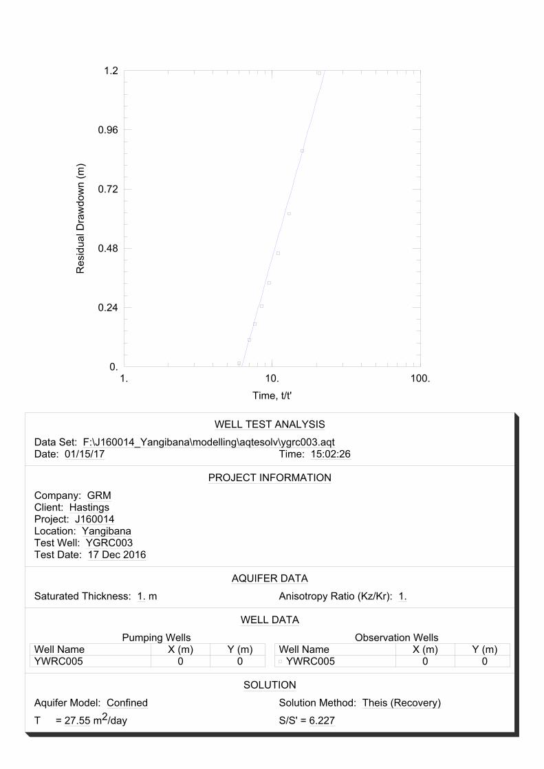
1. 10. 100.0.
0.24
0.48
0.72
0.96
1.2
Time, t/t'
Res
idua
l Dra
wdo
wn
(m)
WELL TEST ANALYSIS
Data Set: F:\J160014_Yangibana\modelling\aqtesolv\ygrc003.aqtDate: 01/15/17 Time: 15:02:26
PROJECT INFORMATION
Company: GRMClient: HastingsProject: J160014Location: YangibanaTest Well: YGRC003Test Date: 17 Dec 2016
AQUIFER DATA
Saturated Thickness: 1. m Anisotropy Ratio (Kz/Kr): 1.
WELL DATA
Pumping WellsWell Name X (m) Y (m)YWRC005 0 0
Observation WellsWell Name X (m) Y (m)
YWRC005 0 0
SOLUTION
Aquifer Model: Confined Solution Method: Theis (Recovery)
T = 27.55 m2/day S/S' = 6.227
J160014R01 E-1 February 2017
APPENDIX E
Laboratory Certificates
Accreditation No. 2562
Date Reported
Contact
SGS Perth Environmental
28 Reid Rd
Perth Airport WA 6105
Ros Ma
(08) 9373 3500
(08) 9373 3556
1
SGS Reference
Facsimile
Telephone
Address
Manager
Laboratory
J160014
Yangibana
9433 2322
9433 2222
PO Box 8110 Fremantle High Street, Fremantle,
WA, 6160
23 Parry Street
Fremantle 6160
KARDINYA WA
Groundwater Resource Management
Kathy McDougall
Samples
Order Number
Project
Facsimile
Telephone
Address
Client
CLIENT DETAILS LABORATORY DETAILS
09 Jan 2017
ANALYTICAL REPORT
PE112997 R0
22 Dec 2016Date Received
Accredited for compliance with ISO/IEC 17025. NATA accredited laboratory 2562(898/20210).
COMMENTS
Donald Smith
Chemist
Michael McKay
Inorganics and ARD Supervisor
Tommy Cheng
ICP Chemist
SIGNATORIES
SGS Australia Pty Ltd
ABN 44 000 964 278
Environment, Health and Safety 28 Reid Rd
PO Box 32
Perth Airport WA 6105
Welshpool WA 6983
Australia
Australia
t +61 8 9373 3500
f +61 8 9373 3556
www.sgs.com.au
Member of the SGS Group
Page 1 of 709-January-2017
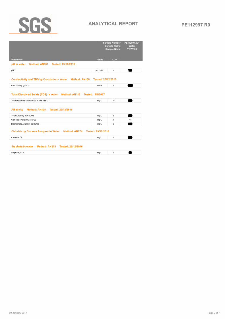
PE112997 R0ANALYTICAL REPORT
PE112997.001
Water
YGWB03
Parameter LORUnits
Sample Number
Sample Matrix
Sample Name
pH in water Method: AN101 Tested: 23/12/2016
pH** pH Units - 7.8
Conductivity and TDS by Calculation - Water Method: AN106 Tested: 23/12/2016
Conductivity @ 25 C µS/cm 2 1500
Total Dissolved Solids (TDS) in water Method: AN113 Tested: 5/1/2017
Total Dissolved Solids Dried at 175-185°C mg/L 10 920
Alkalinity Method: AN135 Tested: 23/12/2016
Total Alkalinity as CaCO3 mg/L 5 270
Carbonate Alkalinity as CO3 mg/L 1 <1
Bicarbonate Alkalinity as HCO3 mg/L 5 330
Chloride by Discrete Analyser in Water Method: AN274 Tested: 29/12/2016
Chloride, Cl mg/L 1 250
Sulphate in water Method: AN275 Tested: 29/12/2016
Sulphate, SO4 mg/L 1 89
Page 2 of 709-January-2017
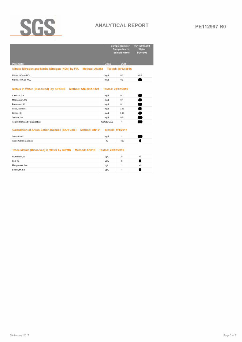
PE112997 R0ANALYTICAL REPORT
PE112997.001
Water
YGWB03
Parameter LORUnits
Sample Number
Sample Matrix
Sample Name
Nitrate Nitrogen and Nitrite Nitrogen (NOx) by FIA Method: AN258 Tested: 28/12/2016
Nitrite, NO₂ as NO₂ mg/L 0.2 <0.2
Nitrate, NO₃ as NO₃ mg/L 0.2 63
Metals in Water (Dissolved) by ICPOES Method: AN320/AN321 Tested: 23/12/2016
Calcium, Ca mg/L 0.2 85
Magnesium, Mg mg/L 0.1 44
Potassium, K mg/L 0.1 7.5
Silica, Soluble mg/L 0.05 91
Silicon, Si mg/L 0.02 43
Sodium, Na mg/L 0.5 180
Total Hardness by Calculation mg CaCO3/L 1 390
Calculation of Anion-Cation Balance (SAR Calc) Method: AN121 Tested: 9/1/2017
Sum of Ions* mg/L - 996
Anion-Cation Balance % -100 1
Trace Metals (Dissolved) in Water by ICPMS Method: AN318 Tested: 28/12/2016
Aluminium, Al µg/L 5 <5
Iron, Fe µg/L 5 5
Manganese, Mn µg/L 1 <1
Selenium, Se µg/L 1 6
Page 3 of 709-January-2017
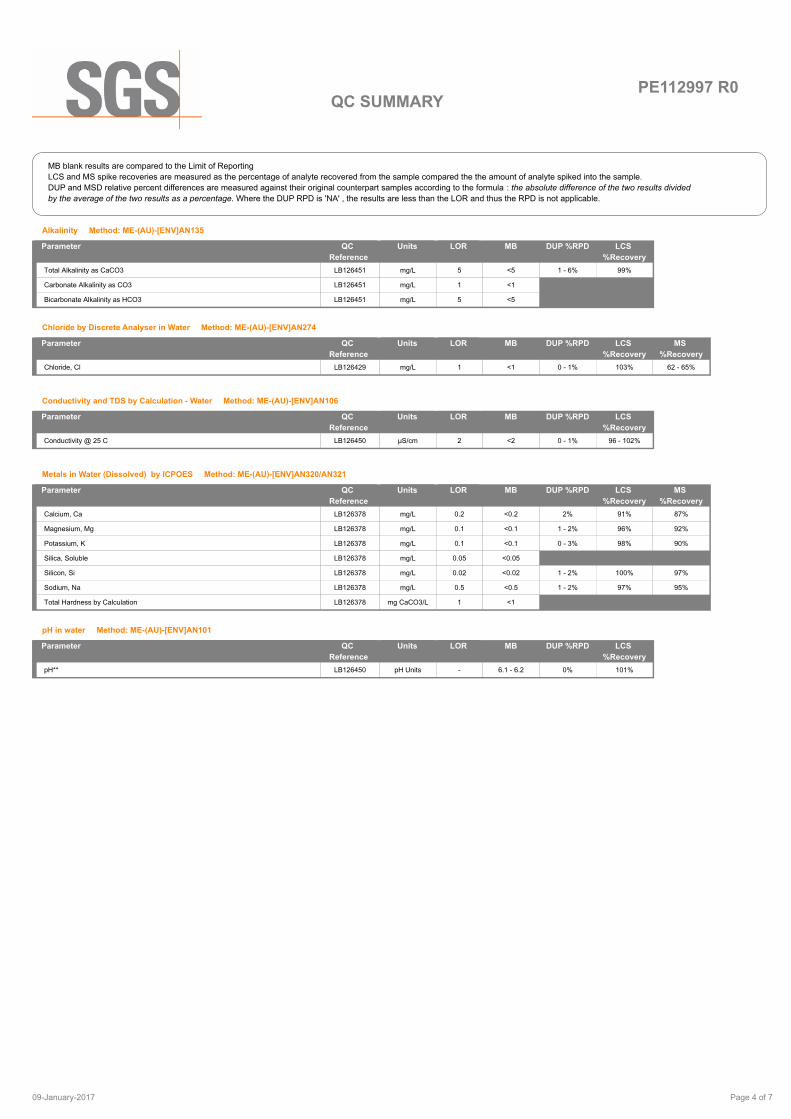
PE112997 R0QC SUMMARY
MB blank results are compared to the Limit of Reporting
LCS and MS spike recoveries are measured as the percentage of analyte recovered from the sample compared the the amount of analyte spiked into the sample.
DUP and MSD relative percent differences are measured against their original counterpart samples according to the formula : the absolute difference of the two results divided
by the average of the two results as a percentage. Where the DUP RPD is 'NA' , the results are less than the LOR and thus the RPD is not applicable.
Alkalinity Method: ME-(AU)-[ENV]AN135
MB DUP %RPD LCS
%Recovery
Total Alkalinity as CaCO3 LB126451 mg/L 5 <5 1 - 6% 99%
Carbonate Alkalinity as CO3 LB126451 mg/L 1 <1
Bicarbonate Alkalinity as HCO3 LB126451 mg/L 5 <5
LORUnits Parameter QC
Reference
Chloride by Discrete Analyser in Water Method: ME-(AU)-[ENV]AN274
MB DUP %RPD LCS
%Recovery
MS
%Recovery
Chloride, Cl LB126429 mg/L 1 <1 0 - 1% 103% 62 - 65%
LORUnits Parameter QC
Reference
Conductivity and TDS by Calculation - Water Method: ME-(AU)-[ENV]AN106
MB DUP %RPD LCS
%Recovery
Conductivity @ 25 C LB126450 µS/cm 2 <2 0 - 1% 96 - 102%
LORUnits Parameter QC
Reference
Metals in Water (Dissolved) by ICPOES Method: ME-(AU)-[ENV]AN320/AN321
MB DUP %RPD LCS
%Recovery
MS
%Recovery
Calcium, Ca LB126378 mg/L 0.2 <0.2 2% 91% 87%
Magnesium, Mg LB126378 mg/L 0.1 <0.1 1 - 2% 96% 92%
Potassium, K LB126378 mg/L 0.1 <0.1 0 - 3% 98% 90%
Silica, Soluble LB126378 mg/L 0.05 <0.05
Silicon, Si LB126378 mg/L 0.02 <0.02 1 - 2% 100% 97%
Sodium, Na LB126378 mg/L 0.5 <0.5 1 - 2% 97% 95%
Total Hardness by Calculation LB126378 mg CaCO3/L 1 <1
LORUnits Parameter QC
Reference
pH in water Method: ME-(AU)-[ENV]AN101
MB DUP %RPD LCS
%Recovery
pH** LB126450 pH Units - 6.1 - 6.2 0% 101%
LORUnits Parameter QC
Reference
Page 4 of 709-January-2017

PE112997 R0QC SUMMARY
MB blank results are compared to the Limit of Reporting
LCS and MS spike recoveries are measured as the percentage of analyte recovered from the sample compared the the amount of analyte spiked into the sample.
DUP and MSD relative percent differences are measured against their original counterpart samples according to the formula : the absolute difference of the two results divided
by the average of the two results as a percentage. Where the DUP RPD is 'NA' , the results are less than the LOR and thus the RPD is not applicable.
Sulphate in water Method: ME-(AU)-[ENV]AN275
MB DUP %RPD LCS
%Recovery
MS
%Recovery
Sulphate, SO4 LB126429 mg/L 1 <1 0 - 1% 103% 83 - 92%
LORUnits Parameter QC
Reference
Total Dissolved Solids (TDS) in water Method: ME-(AU)-[ENV]AN113
MB DUP %RPD LCS
%Recovery
MS
%Recovery
MSD %RPD
Total Dissolved Solids Dried at 175-185°C LB126602 mg/L 10 <10 0 - 1% 93% 103% 4%
LORUnits Parameter QC
Reference
Trace Metals (Dissolved) in Water by ICPMS Method: ME-(AU)-[ENV]AN318
MB DUP %RPD LCS
%Recovery
MS
%Recovery
Aluminium, Al LB126410 µg/L 5 <5 0% 80% 105%
Iron, Fe LB126410 µg/L 5 <5 1% 110% 112%
Manganese, Mn LB126410 µg/L 1 <1 0% 101% 103%
Selenium, Se LB126410 µg/L 1 <1 0% 113% 80%
LORUnits Parameter QC
Reference
Page 5 of 709-January-2017

PE112997 R0
METHOD METHODOLOGY SUMMARY
METHOD SUMMARY
Nitrate and Nitrite by FIA: In an acidic medium, nitrate is reduced quantitatively to nitrite by cadmium metal. This
nitrite plus any original nitrite is determined as an intense red-pink azo dye at 540 nm following diazotisation with
sulphanilamide and subsequent coupling with N-(1-naphthyl) ethylenediamine dihydrochloride. Without the
cadmium reduction only the original nitrite is determined. Reference APHA 4500-NO3- F.
pH in Soil Sludge Sediment and Water: pH is measured electrometrically using a combination electrode (glass plus
reference electrode) and is calibrated against 3 buffers purchased commercially. For soils, an extract with water is
made at a ratio of 1:5 and the pH determined and reported on the extract. Reference APHA 4500-H+.
AN101
Conductivity and TDS by Calculation: Conductivity is measured by meter with temperature compensation and is
calibrated against a standard solution of potassium chloride. Conductivity is generally reported as µmhos/cm or
µS/cm @ 25°C. For soils, an extract with water is made at a ratio of 1:5 and the EC determined and reported on
the extract, or calculated back to the as-received sample. Total Dissolved Salts can be estimated from conductivity
using a conversion factor, which for natural waters, is in the range 0.55 to 0.75. SGS use 0.6. Reference APHA
2510 B.
AN106
Total Dissolved Solids: A well-mixed filtered sample of known volume is evaporated to dryness at 180°C and the
residue weighed. Approximate methods for correlating chemical analysis with dissolved solids are available.
Reference APHA 2540 C.
AN113
This method is used to calculation the balance of major Anions and Cations in water samples and converts major
ion concentration to milliequivalents and then summed. Anions sum and Cation sum is calculated as a difference
and expressed as a percentage.
AN121
The sum of cations and anions in mg/L may also be reported. This sums Na, K, Ca, Mg, NH3, Fe, Cl, Total
Alkalinity, SO4 and NO3.
AN121
Alkalinity (and forms of) by Titration: The sample is titrated with standard acid to pH 8.3 (P titre) and pH 4.5 (T titre)
and permanent and/or total alkalinity calculated. The results are expressed as equivalents of calcium carbonate or
recalculated as bicarbonate, carbonate and hydroxide. Reference APHA 2320. Internal Reference AN135
AN135
Chloride by Aquakem DA: Chloride reacts with mercuric thiocyanate forming a mercuric chloride complex. In the
presence of ferric iron, highly coloured ferric thiocyanate is formed which is proportional to the chloride
concentration. Reference APHA 4500Cl-
AN274
sulfate by Aquakem DA: sulfate is precipitated in an acidic medium with barium chloride. The resulting turbidity is
measured photometrically at 405nm and compared with standard calibration solutions to determine the sulfate
concentration in the sample. Reference APHA 4500-SO42-. Internal reference AN275.
AN275
Determination of elements at trace level in waters by ICP-MS technique, in accordance with USEPA 6020A.AN318
Metals by ICP-OES: Samples are preserved with 10% nitric acid for a wide range of metals and some non-metals.
This solution is measured by Inductively Coupled Plasma. Solutions are aspirated into an argon plasma at
8000-10000K and emit characteristic energy or light as a result of electron transitions through unique energy
levels. The emitted light is focused onto a diffraction grating where it is separated into components .
AN320/AN321
Photomultipliers or CCDs are used to measure the light intensity at specific wavelengths. This intensity is directly
proportional to concentration. Corrections are required to compensate for spectral overlap between elements.
Reference APHA 3120 B.
AN320/AN321
Free and Total Carbon Dioxide may be calculated using alkalinity forms only when the samples TDS is <500mg/L.
If TDS is >500mg/L free or total carbon dioxide cannot be reported . APHA4500CO2 D.
Calculation
Page 6 of 709-January-2017
PE112997 R0
Samples analysed as received.
Solid samples expressed on a dry weight basis.
Where "Total" analyte groups are reported (for example, Total PAHs, Total OC Pesticides) the total will be calculated as the sum of the individual
analytes, with those analytes that are reported as <LOR being assumed to be zero. The summed (Total) limit of reporting is calcuated by summing
the individual analyte LORs and dividing by two. For example, where 16 individual analytes are being summed and each has an LOR of 0.1 mg/kg,
the "Totals" LOR will be 1.6 / 2 (0.8 mg/kg). Where only 2 analytes are being summed, the " Total" LOR will be the sum of those two LORs.
Some totals may not appear to add up because the total is rounded after adding up the raw values.
If reported, measurement uncertainty follow the ± sign after the analytical result and is expressed as the expanded uncertainty calculated using a
coverage factor of 2, providing a level of confidence of approximately 95%, unless stated otherwise in the comments section of this report.
Results reported for samples tested under test methods with codes starting with ARS -SOP, radionuclide or gross radioactivity concentrations are
expressed in becquerel (Bq) per unit of mass or volume or per wipe as stated on the report. Becquerel is the SI unit for activity and equals one
nuclear transformation per second.
Note that in terms of units of radioactivity:
a. 1 Bq is equivalent to 27 pCi
b. 37 MBq is equivalent to 1 mCi
For results reported for samples tested under test methods with codes starting with ARS -SOP, less than (<) values indicate the detection limit for
each radionuclide or parameter for the measurement system used. The respective detection limits have been calculated in accordance with ISO
11929.
The QC criteria are subject to internal review according to the SGS QAQC plan and may be provided on request or alternatively can be found here :
http://www.sgs.com.au/~/media/Local/Australia/Documents/Technical%20Documents/MP-AU-ENV-QU-022%20QA%20QC%20Plan.pdf
This document is issued, on the Client 's behalf, by the Company under its General Conditions of Service available on request and accessible at
http://www.sgs.com/en/terms-and-conditions. The Client's attention is drawn to the limitation of liability, indemnification and jurisdiction issues
defined therein.
Any other holder of this document is advised that information contained hereon reflects the Company 's findings at the time of its intervention only
and within the limits of Client's instructions, if any. The Company's sole responsibility is to its Client and this document does not exonerate parties to
a transaction from exercising all their rights and obligations under the transaction documents.
This report must not be reproduced, except in full.
IS
LNR
*
**
Insufficient sample for analysis.
Sample listed, but not received.
NATA accreditation does not cover the
performance of this service.
Indicative data, theoretical holding time exceeded.
FOOTNOTES
LOR
↑↓
QFH
QFL
-
NVL
Limit of Reporting
Raised or Lowered Limit of Reporting
QC result is above the upper tolerance
QC result is below the lower tolerance
The sample was not analysed for this analyte
Not Validated
Page 7 of 709-January-2017
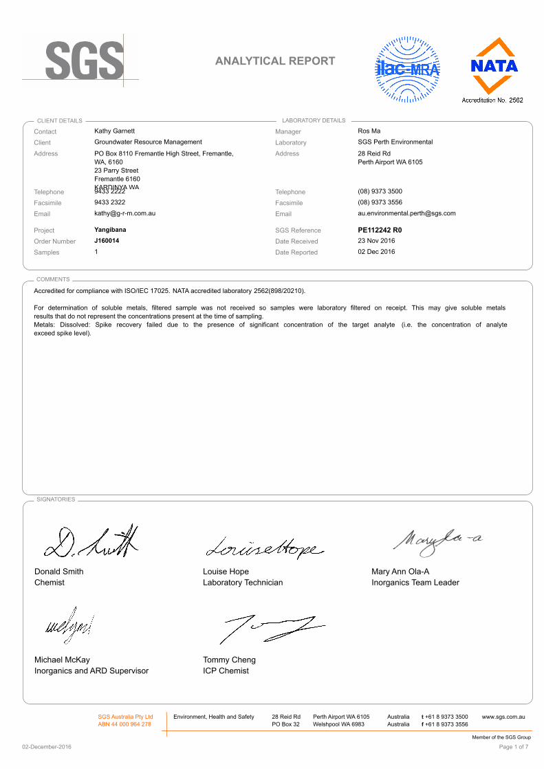
Date Reported
Contact
SGS Perth Environmental
28 Reid Rd
Perth Airport WA 6105
Ros Ma
(08) 9373 3500
(08) 9373 3556
1
SGS Reference
Facsimile
Telephone
Address
Manager
Laboratory
J160014
Yangibana
9433 2322
9433 2222
PO Box 8110 Fremantle High Street, Fremantle,
WA, 6160
23 Parry Street
Fremantle 6160
KARDINYA WA
Groundwater Resource Management
Kathy Garnett
Samples
Order Number
Project
Facsimile
Telephone
Address
Client
CLIENT DETAILS LABORATORY DETAILS
02 Dec 2016
ANALYTICAL REPORT
PE112242 R0
23 Nov 2016Date Received
Accredited for compliance with ISO/IEC 17025. NATA accredited laboratory 2562(898/20210).
For determination of soluble metals, filtered sample was not received so samples were laboratory filtered on receipt. This may give soluble metals
results that do not represent the concentrations present at the time of sampling.
Metals: Dissolved: Spike recovery failed due to the presence of significant concentration of the target analyte (i.e. the concentration of analyte
exceed spike level).
COMMENTS
Donald Smith
Chemist
Louise Hope
Laboratory Technician
Mary Ann Ola-A
Inorganics Team Leader
Michael McKay
Inorganics and ARD Supervisor
Tommy Cheng
ICP Chemist
SIGNATORIES
SGS Australia Pty Ltd
ABN 44 000 964 278
Environment, Health and Safety 28 Reid Rd
PO Box 32
Perth Airport WA 6105
Welshpool WA 6983
Australia
Australia
t +61 8 9373 3500
f +61 8 9373 3556
www.sgs.com.au
Member of the SGS Group
Page 1 of 702-December-2016

PE112242 R0ANALYTICAL REPORT
PE112242.001
Water
06 Nov 2016
FRWI
Parameter LORUnits
Sample Number
Sample Matrix
Sample Date
Sample Name
pH in water Method: AN101 Tested: 23/11/2016
pH** pH Units - 8.5
Conductivity and TDS by Calculation - Water Method: AN106 Tested: 23/11/2016
Conductivity @ 25 C µS/cm 2 2100
Total Dissolved Solids (TDS) in water Method: AN113 Tested: 30/11/2016
Total Dissolved Solids Dried at 175-185°C mg/L 10 1200
Alkalinity Method: AN135 Tested: 23/11/2016
Carbonate Alkalinity as CO3 mg/L 1 11
Bicarbonate Alkalinity as HCO3 mg/L 5 280
Chloride by Discrete Analyser in Water Method: AN274 Tested: 25/11/2016
Chloride, Cl mg/L 1 380
Sulphate in water Method: AN275 Tested: 25/11/2016
Sulphate, SO4 mg/L 1 160
Page 2 of 702-December-2016

PE112242 R0ANALYTICAL REPORT
PE112242.001
Water
06 Nov 2016
FRWI
Parameter LORUnits
Sample Number
Sample Matrix
Sample Date
Sample Name
Nitrate Nitrogen and Nitrite Nitrogen (NOx) by FIA Method: AN258 Tested: 28/11/2016
Nitrate Nitrogen, NO₃ as N mg/L 0.05 9.1
Nitrite, NO₂ as NO₂ mg/L 0.2 <0.2
Metals in Water (Dissolved) by ICPOES Method: AN320/AN321 Tested: 30/11/2016
Calcium, Ca mg/L 0.2 72
Magnesium, Mg mg/L 0.1 67
Potassium, K mg/L 0.1 9.5
Silica, Soluble mg/L 0.05 52
Sodium, Na mg/L 0.5 230
Total Hardness by Calculation mg CaCO3/L 1 460
Trace Metals (Dissolved) in Water by ICPMS Method: AN318 Tested: 29/11/2016
Aluminium, Al µg/L 5 <5
Manganese, Mn µg/L 1 <1
Selenium, Se µg/L 1 4
Trace Metals (Total) in Water by ICPMS Method: AN022/AN318 Tested: 25/11/2016
Total Iron µg/L 5 73
Page 3 of 702-December-2016
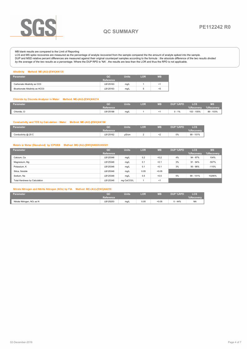
PE112242 R0QC SUMMARY
MB blank results are compared to the Limit of Reporting
LCS and MS spike recoveries are measured as the percentage of analyte recovered from the sample compared the the amount of analyte spiked into the sample.
DUP and MSD relative percent differences are measured against their original counterpart samples according to the formula : the absolute difference of the two results divided
by the average of the two results as a percentage. Where the DUP RPD is 'NA' , the results are less than the LOR and thus the RPD is not applicable.
Alkalinity Method: ME-(AU)-[ENV]AN135
MB
Carbonate Alkalinity as CO3 LB125163 mg/L 1 <1
Bicarbonate Alkalinity as HCO3 LB125163 mg/L 5 <5
LORUnits Parameter QC
Reference
Chloride by Discrete Analyser in Water Method: ME-(AU)-[ENV]AN274
MB DUP %RPD LCS
%Recovery
MS
%Recovery
Chloride, Cl LB125188 mg/L 1 <1 0 - 1% 102 - 105% 89 - 103%
LORUnits Parameter QC
Reference
Conductivity and TDS by Calculation - Water Method: ME-(AU)-[ENV]AN106
MB DUP %RPD LCS
%Recovery
Conductivity @ 25 C LB125162 µS/cm 2 <2 0% 99 - 101%
LORUnits Parameter QC
Reference
Metals in Water (Dissolved) by ICPOES Method: ME-(AU)-[ENV]AN320/AN321
MB DUP %RPD LCS
%Recovery
MS
%Recovery
Calcium, Ca LB125348 mg/L 0.2 <0.2 4% 94 - 97% 104%
Magnesium, Mg LB125348 mg/L 0.1 <0.1 3% 91 - 94% -507%
Potassium, K LB125348 mg/L 0.1 <0.1 3% 95 - 96% -115%
Silica, Soluble LB125348 mg/L 0.05 <0.05
Sodium, Na LB125348 mg/L 0.5 <0.5 5% 99 - 101% 10290%
Total Hardness by Calculation LB125348 mg CaCO3/L 1 <1
LORUnits Parameter QC
Reference
Nitrate Nitrogen and Nitrite Nitrogen (NOx) by FIA Method: ME-(AU)-[ENV]AN258
MB DUP %RPD LCS
%Recovery
Nitrate Nitrogen, NO₃ as N LB125253 mg/L 0.05 <0.05 0 - 44% NA
LORUnits Parameter QC
Reference
Page 4 of 702-December-2016
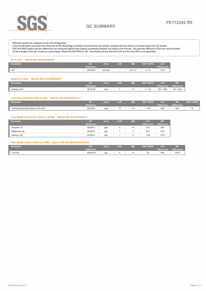
PE112242 R0QC SUMMARY
MB blank results are compared to the Limit of Reporting
LCS and MS spike recoveries are measured as the percentage of analyte recovered from the sample compared the the amount of analyte spiked into the sample.
DUP and MSD relative percent differences are measured against their original counterpart samples according to the formula : the absolute difference of the two results divided
by the average of the two results as a percentage. Where the DUP RPD is 'NA' , the results are less than the LOR and thus the RPD is not applicable.
pH in water Method: ME-(AU)-[ENV]AN101
MB DUP %RPD LCS
%Recovery
pH** LB125162 pH Units - 6.0 - 6.2 0 - 1% 101%
LORUnits Parameter QC
Reference
Sulphate in water Method: ME-(AU)-[ENV]AN275
MB DUP %RPD LCS
%Recovery
MS
%Recovery
Sulphate, SO4 LB125188 mg/L 1 <1 0 - 1% 102 - 106% 100 - 102%
LORUnits Parameter QC
Reference
Total Dissolved Solids (TDS) in water Method: ME-(AU)-[ENV]AN113
MB DUP %RPD LCS
%Recovery
MS
%Recovery
MSD %RPD
Total Dissolved Solids Dried at 175-185°C LB125237 mg/L 10 <10 1 - 6% 96% 95% 1%
LORUnits Parameter QC
Reference
Trace Metals (Dissolved) in Water by ICPMS Method: ME-(AU)-[ENV]AN318
MB LCS
%Recovery
MS
%Recovery
Aluminium, Al LB125311 µg/L 5 <5 81% 99%
Manganese, Mn LB125311 µg/L 1 <1 97% 101%
Selenium, Se LB125311 µg/L 1 <1 114% 122%
LORUnits Parameter QC
Reference
Trace Metals (Total) in Water by ICPMS Method: ME-(AU)-[ENV]AN022/AN318
MB DUP %RPD LCS
%Recovery
MS
%Recovery
Total Iron LB125178 µg/L 5 <5 4% 86% 251%
LORUnits Parameter QC
Reference
Page 5 of 702-December-2016

PE112242 R0
METHOD METHODOLOGY SUMMARY
METHOD SUMMARY
Nitrate and Nitrite by FIA: In an acidic medium, nitrate is reduced quantitatively to nitrite by cadmium metal. This
nitrite plus any original nitrite is determined as an intense red-pink azo dye at 540 nm following diazotisation with
sulphanilamide and subsequent coupling with N-(1-naphthyl) ethylenediamine dihydrochloride. Without the
cadmium reduction only the original nitrite is determined. Reference APHA 4500-NO3- F.
Following acid digestion of un filtered sample, determination of elements at trace level in waters by ICP-MS
technique, in accordance with USEPA 6020A.
AN022/AN318
pH in Soil Sludge Sediment and Water: pH is measured electrometrically using a combination electrode (glass plus
reference electrode) and is calibrated against 3 buffers purchased commercially. For soils, an extract with water is
made at a ratio of 1:5 and the pH determined and reported on the extract. Reference APHA 4500-H+.
AN101
Conductivity and TDS by Calculation: Conductivity is measured by meter with temperature compensation and is
calibrated against a standard solution of potassium chloride. Conductivity is generally reported as µmhos/cm or
µS/cm @ 25°C. For soils, an extract with water is made at a ratio of 1:5 and the EC determined and reported on
the extract, or calculated back to the as-received sample. Total Dissolved Salts can be estimated from conductivity
using a conversion factor, which for natural waters, is in the range 0.55 to 0.75. SGS use 0.6. Reference APHA
2510 B.
AN106
Total Dissolved Solids: A well-mixed filtered sample of known volume is evaporated to dryness at 180°C and the
residue weighed. Approximate methods for correlating chemical analysis with dissolved solids are available.
Reference APHA 2540 C.
AN113
This method is used to calculation the balance of major Anions and Cations in water samples and converts major
ion concentration to milliequivalents and then summed. Anions sum and Cation sum is calculated as a difference
and expressed as a percentage.
AN121
The sum of cations and anions in mg/L may also be reported. This sums Na, K, Ca, Mg, NH3, Fe, Cl, Total
Alkalinity, SO4 and NO3.
AN121
Alkalinity (and forms of) by Titration: The sample is titrated with standard acid to pH 8.3 (P titre) and pH 4.5 (T titre)
and permanent and/or total alkalinity calculated. The results are expressed as equivalents of calcium carbonate or
recalculated as bicarbonate, carbonate and hydroxide. Reference APHA 2320. Internal Reference AN135
AN135
Chloride by Aquakem DA: Chloride reacts with mercuric thiocyanate forming a mercuric chloride complex. In the
presence of ferric iron, highly coloured ferric thiocyanate is formed which is proportional to the chloride
concentration. Reference APHA 4500Cl-
AN274
sulfate by Aquakem DA: sulfate is precipitated in an acidic medium with barium chloride. The resulting turbidity is
measured photometrically at 405nm and compared with standard calibration solutions to determine the sulfate
concentration in the sample. Reference APHA 4500-SO42-. Internal reference AN275.
AN275
Determination of elements at trace level in waters by ICP-MS technique, in accordance with USEPA 6020A.AN318
Metals by ICP-OES: Samples are preserved with 10% nitric acid for a wide range of metals and some non-metals.
This solution is measured by Inductively Coupled Plasma. Solutions are aspirated into an argon plasma at
8000-10000K and emit characteristic energy or light as a result of electron transitions through unique energy
levels. The emitted light is focused onto a diffraction grating where it is separated into components .
AN320/AN321
Photomultipliers or CCDs are used to measure the light intensity at specific wavelengths. This intensity is directly
proportional to concentration. Corrections are required to compensate for spectral overlap between elements.
Reference APHA 3120 B.
AN320/AN321
Free and Total Carbon Dioxide may be calculated using alkalinity forms only when the samples TDS is <500mg/L.
If TDS is >500mg/L free or total carbon dioxide cannot be reported . APHA4500CO2 D.
Calculation
Page 6 of 702-December-2016

PE112242 R0
METHOD METHODOLOGY SUMMARY
METHOD SUMMARY
Samples analysed as received.
Solid samples expressed on a dry weight basis.
Where "Total" analyte groups are reported (for example, Total PAHs, Total OC Pesticides) the total will be calculated as the sum of the individual
analytes, with those analytes that are reported as <LOR being assumed to be zero. The summed (Total) limit of reporting is calcuated by summing
the individual analyte LORs and dividing by two. For example, where 16 individual analytes are being summed and each has an LOR of 0.1 mg/kg,
the "Totals" LOR will be 1.6 / 2 (0.8 mg/kg). Where only 2 analytes are being summed, the " Total" LOR will be the sum of those two LORs.
Some totals may not appear to add up because the total is rounded after adding up the raw values.
If reported, measurement uncertainty follow the ± sign after the analytical result and is expressed as the expanded uncertainty calculated using a
coverage factor of 2, providing a level of confidence of approximately 95%, unless stated otherwise in the comments section of this report.
Results reported for samples tested under test methods with codes starting with ARS -SOP, radionuclide or gross radioactivity concentrations are
expressed in becquerel (Bq) per unit of mass or volume or per wipe as stated on the report. Becquerel is the SI unit for activity and equals one
nuclear transformation per second.
Note that in terms of units of radioactivity:
a. 1 Bq is equivalent to 27 pCi
b. 37 MBq is equivalent to 1 mCi
For results reported for samples tested under test methods with codes starting with ARS -SOP, less than (<) values indicate the detection limit for
each radionuclide or parameter for the measurement system used. The respective detection limits have been calculated in accordance with ISO
11929.
The QC criteria are subject to internal review according to the SGS QAQC plan and may be provided on request or alternatively can be found here :
http://www.sgs.com.au/~/media/Local/Australia/Documents/Technical%20Documents/MP-AU-ENV-QU-022%20QA%20QC%20Plan.pdf
This document is issued, on the Client 's behalf, by the Company under its General Conditions of Service available on request and accessible at
http://www.sgs.com/en/terms-and-conditions. The Client's attention is drawn to the limitation of liability, indemnification and jurisdiction issues
defined therein.
Any other holder of this document is advised that information contained hereon reflects the Company 's findings at the time of its intervention only
and within the limits of Client's instructions, if any. The Company's sole responsibility is to its Client and this document does not exonerate parties to
a transaction from exercising all their rights and obligations under the transaction documents.
This report must not be reproduced, except in full.
IS
LNR
*
**
Insufficient sample for analysis.
Sample listed, but not received.
NATA accreditation does not cover the
performance of this service.
Indicative data, theoretical holding time exceeded.
FOOTNOTES
LOR
↑↓
QFH
QFL
-
NVL
Limit of Reporting
Raised or Lowered Limit of Reporting
QC result is above the upper tolerance
QC result is below the lower tolerance
The sample was not analysed for this analyte
Not Validated
Page 7 of 702-December-2016
Accreditation No. 2562
Date Reported
Contact
SGS Perth Environmental
28 Reid Rd
Perth Airport WA 6105
Ros Ma
(08) 9373 3500
(08) 9373 3556
1
SGS Reference
Facsimile
Telephone
Address
Manager
Laboratory
J160014
Yangibana
9433 2322
9433 2222
PO Box 8110 Fremantle High Street, Fremantle,
WA, 6160
23 Parry Street
Fremantle 6160
KARDINYA WA
Groundwater Resource Management
Kathy McDougall
Samples
Order Number
Project
Facsimile
Telephone
Address
Client
CLIENT DETAILS LABORATORY DETAILS
05 Jan 2017
ANALYTICAL REPORT
PE112957 R0
21 Dec 2016Date Received
Accredited for compliance with ISO/IEC 17025. NATA accredited laboratory 2562(898/20210).
COMMENTS
Donald Smith
Chemist
Hue Thanh Ly
Metals Team Leader
Michael McKay
Inorganics and ARD Supervisor
SIGNATORIES
SGS Australia Pty Ltd
ABN 44 000 964 278
Environment, Health and Safety 28 Reid Rd
PO Box 32
Perth Airport WA 6105
Welshpool WA 6983
Australia
Australia
t +61 8 9373 3500
f +61 8 9373 3556
www.sgs.com.au
Member of the SGS Group
Page 1 of 705-January-2017
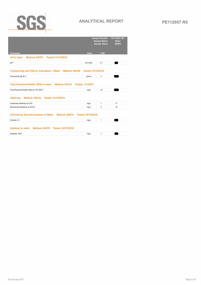
PE112957 R0ANALYTICAL REPORT
PE112957.001
Water
BHW5
Parameter LORUnits
Sample Number
Sample Matrix
Sample Name
pH in water Method: AN101 Tested: 21/12/2016
pH** pH Units 0.1 8.0
Conductivity and TDS by Calculation - Water Method: AN106 Tested: 21/12/2016
Conductivity @ 25 C µS/cm 2 1900
Total Dissolved Solids (TDS) in water Method: AN113 Tested: 3/1/2017
Total Dissolved Solids Dried at 175-185°C mg/L 10 1000
Alkalinity Method: AN135 Tested: 21/12/2016
Carbonate Alkalinity as CO3 mg/L 1 <1
Bicarbonate Alkalinity as HCO3 mg/L 5 <5
Chloride by Discrete Analyser in Water Method: AN274 Tested: 22/12/2016
Chloride, Cl mg/L 1 330
Sulphate in water Method: AN275 Tested: 22/12/2016
Sulphate, SO4 mg/L 1 100
Page 2 of 705-January-2017

PE112957 R0ANALYTICAL REPORT
PE112957.001
Water
BHW5
Parameter LORUnits
Sample Number
Sample Matrix
Sample Name
Low Level Nitrate Nitrogen and Nitrite Nitrogen (NOx) by FIA Method: AN258 Tested: 22/12/2016
Nitrate, NO₃ as NO₃ mg/L 0.05 65
Nitrite, NO₂ as NO₂ mg/L 0.05 <0.05
Metals in Water (Dissolved) by ICPOES Method: AN320/AN321 Tested: 21/12/2016
Calcium, Ca mg/L 0.2 81
Magnesium, Mg mg/L 0.1 51
Potassium, K mg/L 0.1 9.0
Silica, Soluble mg/L 0.05 72
Silicon, Si mg/L 0.02 34
Sodium, Na mg/L 0.5 240
Total Hardness by Calculation mg CaCO3/L 1 410
Trace Metals (Dissolved) in Water by ICPMS Method: AN318 Tested: 21/12/2016
Aluminium, Al µg/L 5 <5
Iron, Fe µg/L 5 9
Manganese, Mn µg/L 1 <1
Selenium, Se µg/L 1 7
Page 3 of 705-January-2017
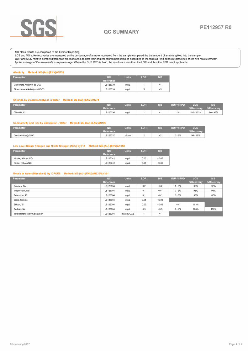
PE112957 R0QC SUMMARY
MB blank results are compared to the Limit of Reporting
LCS and MS spike recoveries are measured as the percentage of analyte recovered from the sample compared the the amount of analyte spiked into the sample.
DUP and MSD relative percent differences are measured against their original counterpart samples according to the formula : the absolute difference of the two results divided
by the average of the two results as a percentage. Where the DUP RPD is 'NA' , the results are less than the LOR and thus the RPD is not applicable.
Alkalinity Method: ME-(AU)-[ENV]AN135
MB
Carbonate Alkalinity as CO3 LB126339 mg/L 1 <1
Bicarbonate Alkalinity as HCO3 LB126339 mg/L 5 <5
LORUnits Parameter QC
Reference
Chloride by Discrete Analyser in Water Method: ME-(AU)-[ENV]AN274
MB DUP %RPD LCS
%Recovery
MS
%Recovery
Chloride, Cl LB126336 mg/L 1 <1 1% 102 - 103% 80 - 96%
LORUnits Parameter QC
Reference
Conductivity and TDS by Calculation - Water Method: ME-(AU)-[ENV]AN106
MB DUP %RPD LCS
%Recovery
Conductivity @ 25 C LB126337 µS/cm 2 <2 0 - 2% 96 - 99%
LORUnits Parameter QC
Reference
Low Level Nitrate Nitrogen and Nitrite Nitrogen (NOx) by FIA Method: ME-(AU)-[ENV]AN258
MB
Nitrate, NO₃ as NO₃ LB126342 mg/L 0.05 <0.05
Nitrite, NO₂ as NO₂ LB126342 mg/L 0.05 <0.05
LORUnits Parameter QC
Reference
Metals in Water (Dissolved) by ICPOES Method: ME-(AU)-[ENV]AN320/AN321
MB DUP %RPD LCS
%Recovery
MS
%Recovery
Calcium, Ca LB126304 mg/L 0.2 <0.2 1 - 3% 95% 92%
Magnesium, Mg LB126304 mg/L 0.1 <0.1 0 - 3% 98% 93%
Potassium, K LB126304 mg/L 0.1 <0.1 0 - 3% 95% 87%
Silica, Soluble LB126304 mg/L 0.05 <0.05
Silicon, Si LB126304 mg/L 0.02 <0.02 0% 103%
Sodium, Na LB126304 mg/L 0.5 <0.5 1 - 4% 108% 100%
Total Hardness by Calculation LB126304 mg CaCO3/L 1 <1
LORUnits Parameter QC
Reference
Page 4 of 705-January-2017
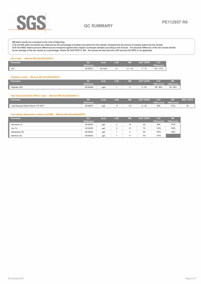
PE112957 R0QC SUMMARY
MB blank results are compared to the Limit of Reporting
LCS and MS spike recoveries are measured as the percentage of analyte recovered from the sample compared the the amount of analyte spiked into the sample.
DUP and MSD relative percent differences are measured against their original counterpart samples according to the formula : the absolute difference of the two results divided
by the average of the two results as a percentage. Where the DUP RPD is 'NA' , the results are less than the LOR and thus the RPD is not applicable.
pH in water Method: ME-(AU)-[ENV]AN101
MB DUP %RPD LCS
%Recovery
pH** LB126337 pH Units 0.1 5.7 - 6.0 0 - 1% 100 - 101%
LORUnits Parameter QC
Reference
Sulphate in water Method: ME-(AU)-[ENV]AN275
MB DUP %RPD LCS
%Recovery
MS
%Recovery
Sulphate, SO4 LB126336 mg/L 1 <1 0 - 2% 98 - 99% 90 - 94%
LORUnits Parameter QC
Reference
Total Dissolved Solids (TDS) in water Method: ME-(AU)-[ENV]AN113
MB DUP %RPD LCS
%Recovery
MS
%Recovery
MSD %RPD
Total Dissolved Solids Dried at 175-185°C LB126510 mg/L 10 <10 0 - 2% 89% 101% 3%
LORUnits Parameter QC
Reference
Trace Metals (Dissolved) in Water by ICPMS Method: ME-(AU)-[ENV]AN318
MB DUP %RPD LCS
%Recovery
MS
%Recovery
Aluminium, Al LB126303 µg/L 5 <5 0% 99% 107%
Iron, Fe LB126303 µg/L 5 <5 7% 103% 109%
Manganese, Mn LB126303 µg/L 1 <1 0% 100% 105%
Selenium, Se LB126303 µg/L 1 <1 0% 107%
LORUnits Parameter QC
Reference
Page 5 of 705-January-2017

PE112957 R0
METHOD METHODOLOGY SUMMARY
METHOD SUMMARY
pH in Soil Sludge Sediment and Water: pH is measured electrometrically using a combination electrode (glass plus
reference electrode) and is calibrated against 3 buffers purchased commercially. For soils, an extract with water is
made at a ratio of 1:5 and the pH determined and reported on the extract. Reference APHA 4500-H+.
AN101
Conductivity and TDS by Calculation: Conductivity is measured by meter with temperature compensation and is
calibrated against a standard solution of potassium chloride. Conductivity is generally reported as µmhos/cm or
µS/cm @ 25°C. For soils, an extract with water is made at a ratio of 1:5 and the EC determined and reported on
the extract, or calculated back to the as-received sample. Total Dissolved Salts can be estimated from conductivity
using a conversion factor, which for natural waters, is in the range 0.55 to 0.75. SGS use 0.6. Reference APHA
2510 B.
AN106
Total Dissolved Solids: A well-mixed filtered sample of known volume is evaporated to dryness at 180°C and the
residue weighed. Approximate methods for correlating chemical analysis with dissolved solids are available.
Reference APHA 2540 C.
AN113
Alkalinity (and forms of) by Titration: The sample is titrated with standard acid to pH 8.3 (P titre) and pH 4.5 (T titre)
and permanent and/or total alkalinity calculated. The results are expressed as equivalents of calcium carbonate or
recalculated as bicarbonate, carbonate and hydroxide. Reference APHA 2320. Internal Reference AN135
AN135
Nitrate and Nitrite by FIA: In an acidic medium, nitrate is reduced quantitatively to nitrite by cadmium metal. This
nitrite plus any original nitrite is determined as an intense red-pink azo dye at 540 nm following diazotisation with
sulphanilamide and subsequent coupling with N-(1-naphthyl) ethylenediamine dihydrochloride. Without the
cadmium reduction only the original nitrite is determined. Reference APHA 4500-NO3- F.
AN258
Chloride by Aquakem DA: Chloride reacts with mercuric thiocyanate forming a mercuric chloride complex. In the
presence of ferric iron, highly coloured ferric thiocyanate is formed which is proportional to the chloride
concentration. Reference APHA 4500Cl-
AN274
sulfate by Aquakem DA: sulfate is precipitated in an acidic medium with barium chloride. The resulting turbidity is
measured photometrically at 405nm and compared with standard calibration solutions to determine the sulfate
concentration in the sample. Reference APHA 4500-SO42-. Internal reference AN275.
AN275
Determination of elements at trace level in waters by ICP-MS technique, in accordance with USEPA 6020A.AN318
Metals by ICP-OES: Samples are preserved with 10% nitric acid for a wide range of metals and some non-metals.
This solution is measured by Inductively Coupled Plasma. Solutions are aspirated into an argon plasma at
8000-10000K and emit characteristic energy or light as a result of electron transitions through unique energy
levels. The emitted light is focused onto a diffraction grating where it is separated into components .
AN320/AN321
Photomultipliers or CCDs are used to measure the light intensity at specific wavelengths. This intensity is directly
proportional to concentration. Corrections are required to compensate for spectral overlap between elements.
Reference APHA 3120 B.
AN320/AN321
Free and Total Carbon Dioxide may be calculated using alkalinity forms only when the samples TDS is <500mg/L.
If TDS is >500mg/L free or total carbon dioxide cannot be reported . APHA4500CO2 D.
Calculation
Page 6 of 705-January-2017

PE112957 R0
Samples analysed as received.
Solid samples expressed on a dry weight basis.
Where "Total" analyte groups are reported (for example, Total PAHs, Total OC Pesticides) the total will be calculated as the sum of the individual
analytes, with those analytes that are reported as <LOR being assumed to be zero. The summed (Total) limit of reporting is calcuated by summing
the individual analyte LORs and dividing by two. For example, where 16 individual analytes are being summed and each has an LOR of 0.1 mg/kg,
the "Totals" LOR will be 1.6 / 2 (0.8 mg/kg). Where only 2 analytes are being summed, the " Total" LOR will be the sum of those two LORs.
Some totals may not appear to add up because the total is rounded after adding up the raw values.
If reported, measurement uncertainty follow the ± sign after the analytical result and is expressed as the expanded uncertainty calculated using a
coverage factor of 2, providing a level of confidence of approximately 95%, unless stated otherwise in the comments section of this report.
Results reported for samples tested under test methods with codes starting with ARS -SOP, radionuclide or gross radioactivity concentrations are
expressed in becquerel (Bq) per unit of mass or volume or per wipe as stated on the report. Becquerel is the SI unit for activity and equals one
nuclear transformation per second.
Note that in terms of units of radioactivity:
a. 1 Bq is equivalent to 27 pCi
b. 37 MBq is equivalent to 1 mCi
For results reported for samples tested under test methods with codes starting with ARS -SOP, less than (<) values indicate the detection limit for
each radionuclide or parameter for the measurement system used. The respective detection limits have been calculated in accordance with ISO
11929.
The QC criteria are subject to internal review according to the SGS QAQC plan and may be provided on request or alternatively can be found here :
http://www.sgs.com.au/~/media/Local/Australia/Documents/Technical%20Documents/MP-AU-ENV-QU-022%20QA%20QC%20Plan.pdf
This document is issued, on the Client 's behalf, by the Company under its General Conditions of Service available on request and accessible at
http://www.sgs.com/en/terms-and-conditions. The Client's attention is drawn to the limitation of liability, indemnification and jurisdiction issues
defined therein.
Any other holder of this document is advised that information contained hereon reflects the Company 's findings at the time of its intervention only
and within the limits of Client's instructions, if any. The Company's sole responsibility is to its Client and this document does not exonerate parties to
a transaction from exercising all their rights and obligations under the transaction documents.
This report must not be reproduced, except in full.
IS
LNR
*
**
Insufficient sample for analysis.
Sample listed, but not received.
NATA accreditation does not cover the
performance of this service.
Indicative data, theoretical holding time exceeded.
FOOTNOTES
LOR
↑↓
QFH
QFL
-
NVL
Limit of Reporting
Raised or Lowered Limit of Reporting
QC result is above the upper tolerance
QC result is below the lower tolerance
The sample was not analysed for this analyte
Not Validated
Page 7 of 705-January-2017


![HS9L]PL^ FREMANTLE 24 hours a day, PORTS...VIC 3003 Australia Tel: +61 3 9680 0700 DP World Fremantle 1 Port Beach Road North Fremantle WA 6159 Australia Tel: +61 8 9430 0111 ... [YHKL](https://img.pdfslide.us/doc/110x75/5f0cf2417e708231d437e9ce/hs9lpl-fremantle-24-hours-a-day-ports-vic-3003-australia-tel-61-3-9680.jpg)