APPENDIX 2 DERIVATION OF THE QUARTERLY DCF MODEL

APPENDIX 2-1

APPENDIX 2

DERIVATION OF THE QUARTERLY DCF MODEL

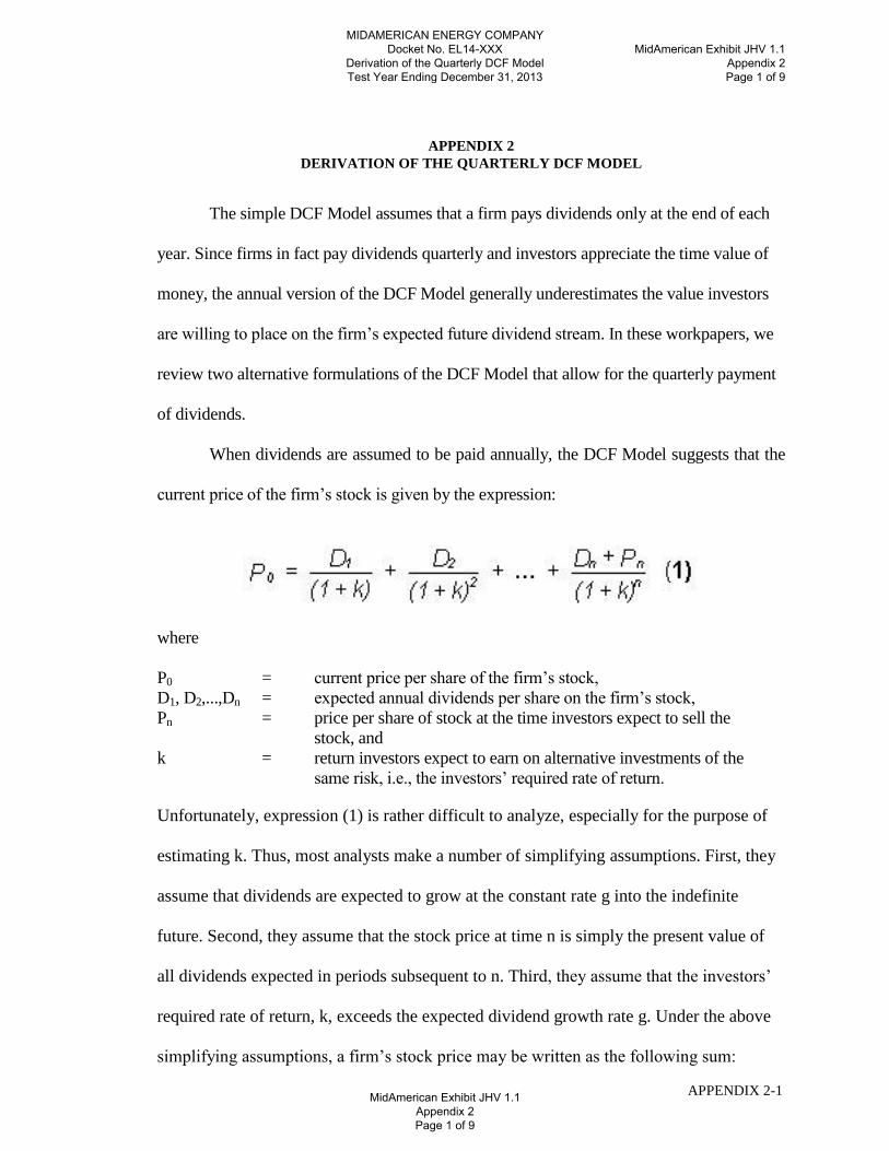
The simple DCF Model assumes that a firm pays dividends only at the end of each

year. Since firms in fact pay dividends quarterly and investors appreciate the time value of

money, the annual version of the DCF Model generally underestimates the value investors

are willing to place on the firm’s expected future dividend stream. In these workpapers, we

review two alternative formulations of the DCF Model that allow for the quarterly payment

of dividends.

When dividends are assumed to be paid annually, the DCF Model suggests that the

current price of the firm’s stock is given by the expression:

where

P0 = current price per share of the firm’s stock,

D1, D2,...,Dn = expected annual dividends per share on the firm’s stock,

Pn = price per share of stock at the time investors expect to sell the

stock, and

k = return investors expect to earn on alternative investments of the

same risk, i.e., the investors’ required rate of return.

Unfortunately, expression (1) is rather difficult to analyze, especially for the purpose of

estimating k. Thus, most analysts make a number of simplifying assumptions. First, they

assume that dividends are expected to grow at the constant rate g into the indefinite

future. Second, they assume that the stock price at time n is simply the present value of

all dividends expected in periods subsequent to n. Third, they assume that the investors’

required rate of return, k, exceeds the expected dividend growth rate g. Under the above

simplifying assumptions, a firm’s stock price may be written as the following sum:

MIDAMERICAN ENERGY COMPANY Docket No. EL14-XXX

Derivation of the Quarterly DCF Model Test Year Ending December 31, 2013

MidAmerican Exhibit JHV 1.1 Appendix 2 Page 1 of 9


APPENDIX 2-2

where the three dots indicate that the sum continues indefinitely.

As we shall demonstrate shortly, this sum may be simplified to:

g)-(k

g)+(1D = P

00

First, however, we need to review the very useful concept of a geometric progression.

Geometric Progression

Consider the sequence of numbers 3, 6, 12, 24,…, where each number after the first

is obtained by multiplying the preceding number by the factor 2. Obviously, this sequence

of numbers may also be expressed as the sequence 3, 3 x 2, 3 x 22, 3 x 2

3, etc. This sequence

is an example of a geometric progression.

Definition: A geometric progression is a sequence in which each term after the first

is obtained by multiplying some fixed number, called the common ratio, by the preceding

term.

A general notation for geometric progressions is: a, the first term, r, the common

ratio, and n, the number of terms. Using this notation, any geometric progression may be

represented by the sequence:

a, ar, ar2, ar

3,…, ar

n-1.

In studying the DCF Model, we will find it useful to have an expression for the sum of n

terms of a geometric progression. Call this sum Sn. Then

However, this expression can be simplified by multiplying both sides of equation (3) by r

and then subtracting the new equation from the old. Thus,





APPENDIX 2-3

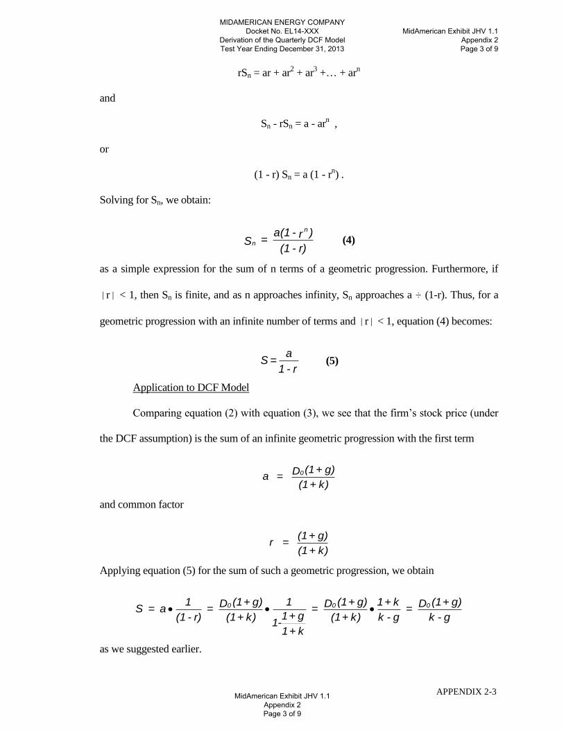
rSn = ar + ar2 + ar

3 +… + ar

n

and

Sn - rSn = a - arn ,

or

(1 - r) Sn = a (1 - rn) .

Solving for Sn, we obtain:

r)-(1

)r-a(1 = S

n

n (4)

as a simple expression for the sum of n terms of a geometric progression. Furthermore, if

|r| < 1, then Sn is finite, and as n approaches infinity, Sn approaches a ÷ (1-r). Thus, for a

geometric progression with an infinite number of terms and |r| < 1, equation (4) becomes:

r- 1

a =S (5)

Application to DCF Model

Comparing equation (2) with equation (3), we see that the firm’s stock price (under

the DCF assumption) is the sum of an infinite geometric progression with the first term

k)+(1

g)+(1D = a 0

and common factor

k)+(1

g)+(1 = r

Applying equation (5) for the sum of such a geometric progression, we obtain

g-k

g)+(1D =

g-k

k+1

k)+(1

g)+(1D =

k+1

g+1-1

1

k)+(1

g)+(1D =

r)-(1

1 a =S 000

as we suggested earlier.





APPENDIX 2-4

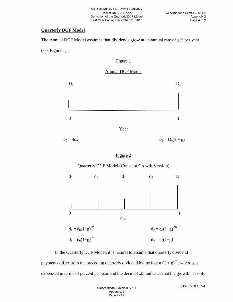
Quarterly DCF Model

The Annual DCF Model assumes that dividends grow at an annual rate of g% per year

(see Figure 1).

Figure 1

Annual DCF Model

D0 D1

0 1

Year

D0 = 4d0 D1 = D0(1 + g)

Figure 2

Quarterly DCF Model (Constant Growth Version)

d0 d1 d2 d3 D1

0 1

Year

d1 = d0(1+g).25

d2 = d0(1+g).50

d3 = d0(1+g).75

d4 = d0(1+g)

In the Quarterly DCF Model, it is natural to assume that quarterly dividend

payments differ from the preceding quarterly dividend by the factor (1 + g).25

, where g is

expressed in terms of percent per year and the decimal .25 indicates that the growth has only





APPENDIX 2-5

occurred for one quarter of the year. (See Figure 2.) Using this assumption, along with the

assumption of constant growth and k > g, we obtain a new expression for the firm’s stock

price, which takes account of the quarterly payment of dividends. This expression is:

where d0 is the last quarterly dividend payment, rather than the last annual dividend

payment. (We use a lower case d to remind the reader that this is not the annual dividend.)

Although equation (6) looks formidable at first glance, it too can be greatly

simplified using the formula [equation (4)] for the sum of an infinite geometric progression.

As the reader can easily verify, equation (6) can be simplified to:

)g+(1- )k+(1

)g+(1d = P

4

1

4

1

4

1

00 (7)

Solving equation (7) for k, we obtain a DCF formula for estimating the cost of equity

under the quarterly dividend assumption:

1 - )g+(1 + P

)g+(1d = k 4

1

0

4

1

0

4

(8)





APPENDIX 2-6

An Alternative Quarterly DCF Model

Although the constant growth Quarterly DCF Model [equation (8)] allows for the

quarterly timing of dividend payments, it does require the assumption that the firm increases

its dividend payments each quarter. Since this assumption is difficult for some analysts to

accept, we now discuss a second Quarterly DCF Model that allows for constant quarterly

dividend payments within each dividend year.

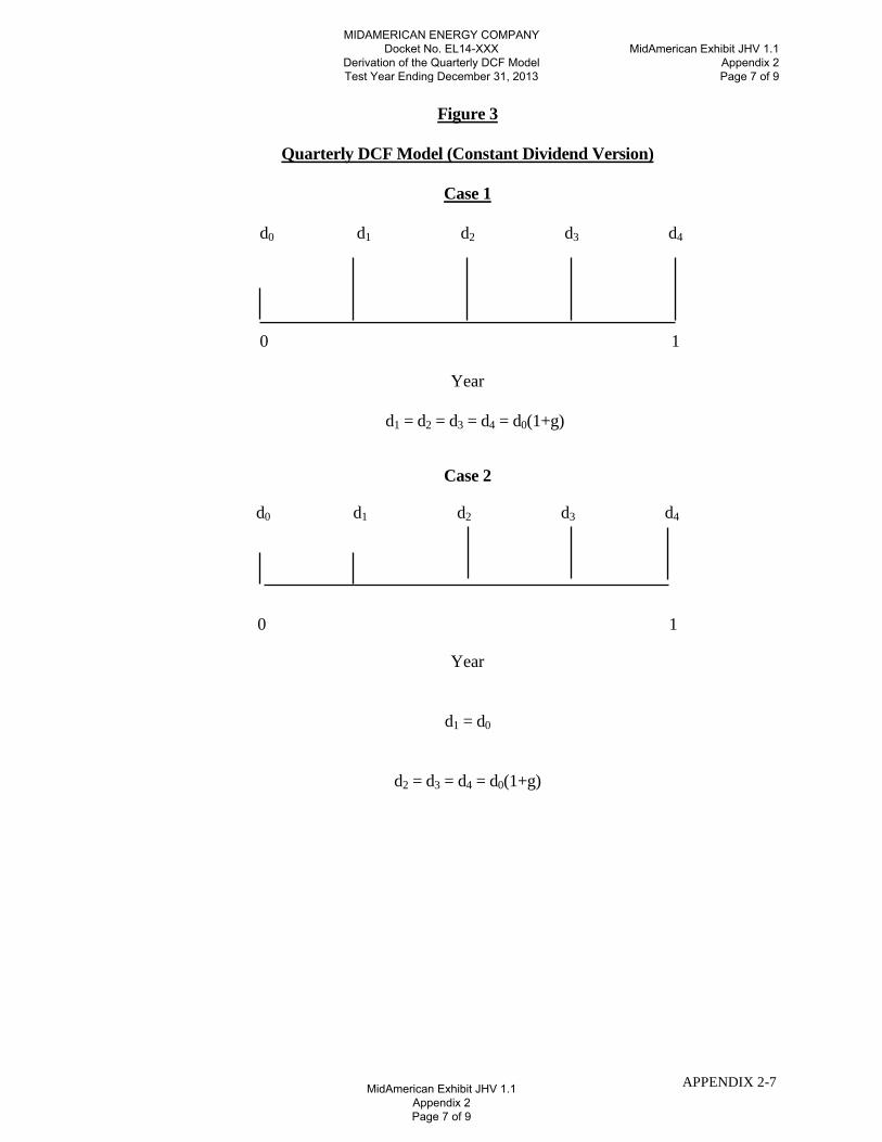
Assume then that the firm pays dividends quarterly and that each dividend payment

is constant for four consecutive quarters. There are four cases to consider, with each case

distinguished by varying assumptions about where we are evaluating the firm in relation to

the time of its next dividend increase. (See Figure 3.)





APPENDIX 2-7

Figure 3

Quarterly DCF Model (Constant Dividend Version)

Case 1

d0 d1 d2 d3 d4

0 1

Year

d1 = d2 = d3 = d4 = d0(1+g)

Case 2

d0 d1 d2 d3 d4

0 1

Year

d1 = d0

d2 = d3 = d4 = d0(1+g)





APPENDIX 2-8

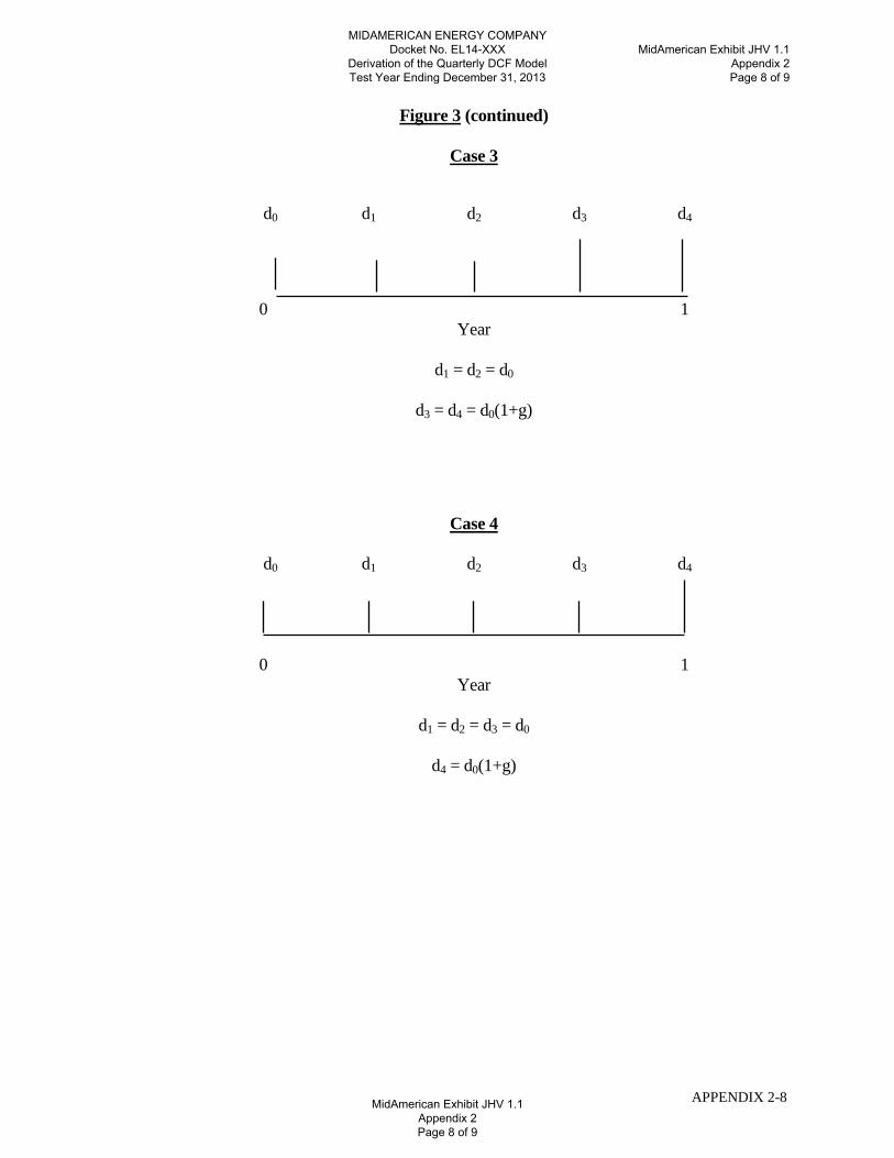
Figure 3 (continued)

Case 3

d0 d1 d2 d3 d4

0 1

Year

d1 = d2 = d0

d3 = d4 = d0(1+g)

Case 4

d0 d1 d2 d3 d4

0 1

Year

d1 = d2 = d3 = d0

d4 = d0(1+g)





APPENDIX 2-9

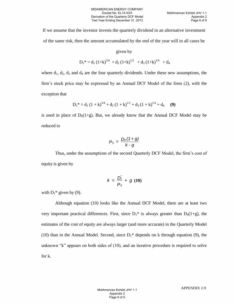
If we assume that the investor invests the quarterly dividend in an alternative investment

of the same risk, then the amount accumulated by the end of the year will in all cases be

given by

D1* = d1 (1+k)3/4

+ d2 (1+k)1/2

+ d3 (1+k)1/4

+ d4

where d1, d2, d3 and d4 are the four quarterly dividends. Under these new assumptions, the

firm’s stock price may be expressed by an Annual DCF Model of the form (2), with the

exception that

D1* = d1 (1 + k)3/4

+ d2 (1 + k)1/2

+ d3 (1 + k)1/4

+ d4 (9)

is used in place of D0(1+g). But, we already know that the Annual DCF Model may be

reduced to

g-k

g)+(1D = P

00

Thus, under the assumptions of the second Quarterly DCF Model, the firm’s cost of

equity is given by

g + P

D = k

0

*1

(10)

with D1* given by (9).

Although equation (10) looks like the Annual DCF Model, there are at least two

very important practical differences. First, since D1* is always greater than D0(1+g), the

estimates of the cost of equity are always larger (and more accurate) in the Quarterly Model

(10) than in the Annual Model. Second, since D1* depends on k through equation (9), the

unknown ―k‖ appears on both sides of (10), and an iterative procedure is required to solve

for k.





Documents

APPENDIX 2 DERIVATION OF THE QUARTERLY DCF MODEL