Appendix 10 - NTEPA · Appendix 10 Wastewater discharge modelling. ICHTHYS GAS FIELD DEVELOPMENT PROJECT WASTEWATER DISCHARGE MODELLING Prepared for INPEX Browse, Ltd. May 2009 INPEX

Appendix 10 Wastewater discharge modelling

ICHTHYS GAS FIELD DEVELOPMENT PROJECT WASTEWATER DISCHARGE MODELLING

Prepared for INPEX Browse, Ltd.

May 2009

INPEX Document No. C036-AH-REP-0002

Asia-Pacific Applied Science Associates www.apasa.com.au

Page ii

Document control form

Document draft

Originated by Edit & review Authorized for release by

Date

Version 2 - Issued for use

Dr Oleg Makarynskyy

Dr Sasha Zigic

22nd May 2009

Document name: INPEX-Darwin-report-discharges_version2 - Final.doc

APASA Project Number: J0036

APASA Project Manager: Sasha Zigic

DISCLAIMER:

This document contains confidential information that is intended only for use by the client and is not for public circulation, publication, nor any third party use without the approval of the client.

Readers should understand that modelling is predictive in nature and while this report is based on information from sources that Asia-Pacific ASA Pty Ltd. considers reliable, the accuracy and completeness of said information cannot be guaranteed. Therefore, Asia-Pacific ASA Pty Ltd., its directors, and employees accept no liability for the result of any action taken or not taken on the basis of the information given in this report, nor for any negligent misstatements, errors, and omissions. This report was compiled with consideration for the specified client's objectives, situation, and needs. Those acting upon such information without first consulting Asia-Pacific ASA Pty Ltd., do so entirely at their own risk.

This report may be cited as:

Asia-Pacific Applied Science Associates. 2009. Ichthys Gas Field Development Project: wastewater discharge modelling. Report prepared for INPEX Browse, Ltd., Perth, Western Australia.


Page iii

Content EXECUTIVE SUMMARY.......................................................................................................... vi

1 INTRODUCTION................................................................................................................1

Scope of work ........................................................................................................................2

2 DEVELOPMENT OF HYDRODYNAMIC DATA.................................................................4

Hydrodynamic model .............................................................................................................4

Existing grid setup and bathymetry ....................................................................................4

Tidal Forcing ......................................................................................................................8

Tidal model validation ........................................................................................................8

Wind Forcing ....................................................................................................................11

Current validation .............................................................................................................12

Current data at the proposed release site ...........................................................................14

3 TREATED WASTEWATER PROPERTIES .....................................................................16

4 TPH-In-Harbour Water Trigger Value ..............................................................................17

5 NEAR FIELD MODELLING..............................................................................................18

Model Description ................................................................................................................18

Ambient Environmental Conditions......................................................................................18

Diffuser design.....................................................................................................................19

Sensitivity testing .................................................................................................................20

Near-Field Results ...............................................................................................................22

6 FAR-FIELD MODELLING ................................................................................................25

Background..........................................................................................................................25

Scenarios.............................................................................................................................25

Far-Field Model....................................................................................................................25

Discharge Input Data ...........................................................................................................26

MUDMAP Mixing Parameters..............................................................................................27

MUDMAP Grid Configuration...............................................................................................27

Far-Field Results .................................................................................................................27

7 CONCLUSIONS AND RECOMMENDATIONS................................................................34

8 REFERENCES.................................................................................................................35


Page iv

Figures Figure 1: Location of the proposed wastewater release site within East Arm, Darwin. .............2

Figure 2: Boundary fitted model grid of Darwin Harbour and tributaries; and (bottom) zoomed in view of East Arm. ...........................................................................................................6

Figure 3: Bathymetric grid used to define the shape of the seabed within the model domain. Top panel shows the entire domain. Lower panel shows a zoom over East Arm. All depths are in highest astronomical tide (HAT). ..................................................................7

Figure 4: Location of pressure gauging stations within East Arm. ............................................8

Figure 5: Inter-comparisons of measured and predicted tidal elevations: Results are shown for Gauge 1 (top panel) and Gauge 2 (bottom panel). .......................................................9

Figure 6: Inter-comparisons of measured and predicted tidal elevations: Results are shown for Gauge 3 (top panel) and Gauge 4 (bottom panel). .....................................................10

Figure 7: Time-series graphs showing the comparison between the winds measured at East Arm Wharf and Darwin Airport: U-component (east-west direction) in top panel and V-component (north-south direction) in bottom panel..........................................................11

Figure 8: Locations of current and wind measurements used to validate current predictions.12

Figure 9: Comparison of currents observed at Sentinel 1 site and simulated by BFHYDRO three-dimensional surface layer (top panel), mid-layer (middle panel) and bottom layer (bottom panel). .................................................................................................................13

Figure 10: Details of bathymetry amended to include the dredged region for the proposed jetty loading facility. ..........................................................................................................14

Figure 11: Current roses for near surface currents (top panels) during wet and dry seasons and corresponding current speeds as a function of time (bottom panels). ......................15

Figure 12. Near-field dilution comparison as function of static average current speed, 4 ports, 0.1 m port diameter, varying spacing during wet conditions ............................................21

Figure 13. Near-field dilution results comparison as function of static average current speed, varying ports, 0.1 m port diameter, 5 m spacing during wet conditions ...........................21

Figure 14. Comparison of the near-field dilutions for a 0.1 m and 0.2 m port diameters, four ports, 5 m spacing, under a range of static current speeds at the proposed jetty during the wet season.................................................................................................................22

Figure 15: Dry season case (18 m3/hr flow rate, 0.2 mg/L TPH) - near-field initial dilution results as a function of static current speeds. ..................................................................24

Figure 16: Wet season case (160 m3/hr, 10 mg/L TPH) - near-field initial dilution results as function of static current speeds. .....................................................................................24


Page v

Figure 17: Example time series of the maximum predicted in-water TPH concentrations (mg/L, 160 m3/hr discharge with 10 mg/L TPH concentration), January 2007 current conditions .........................................................................................................................29

Figure 18: Time series graph (top) of the predicted maximum in-water TPH concentrations (mg/L, 160 m3/hr discharge with 10 mg/L TPH concentration) at the proposed outfall location and corresponding surface current speeds (bottom) for January 2007. .............30

Figure 19: Time series graphs of the predicted maximum in-water TPH concentrations (mg/L) at 100 m (top), 200 m (middle) and 300 m (bottom) west of the release site...................31

Figure 20: Predicted 50th (top); and 95th (bottom) percentiles of TPH concentrations (mg/L, 160 m3/hr discharge with 10 mg/L TPH concentration), January to April 2007 current conditions .........................................................................................................................33

Tables Table 1: Summary of the wastewater characteristics for each season. ..................................16

Table 2. Temperature and salinity used as input into the near field model .............................19

Table 3. Ambient current conditions........................................................................................19

Table 4. Summary of the outfall configurations examined as part of the near-field modelling 20

Table 5. Summary of the final near field modelling results for a 4 port, 5 m spacing 0.1 m diameter diffuser configuration.........................................................................................23

Table 6: Summary of the far-field model settings used to simulate the wastewater discharge during wet season conditions...........................................................................................27

Table 7: Predicted area of coverage and maximum distance for the 50th and 95th percentile concentrations..................................................................................................................32

STUDY DATUMS

Water depths and levels presented in this report are with respect to Mean Sea Level (MSL) unless otherwise stated and are in units of meters.

Positions are satellite derived from the Global Positioning System using the WGS 1984 datum, unless stated otherwise. Position units are in latitude/longitudes.

All units are in standard SI units.


Page vi

EXECUTIVE SUMMARY

INPEX Browse Ltd is to build an onshore processing facility at Blaydin Point in Darwin. The treated wastewater from the plant is to be discharged via an outfall at the western extent of the proposed loading jetty, approximately 1 m above the seabed (~14 m water depth at LAT post dredging).

The wastewater will consist of treated effluent and storm water, and as such will have a slightly elevated temperature (~2 °C), salinity levels will be much lower (approximately 1 ppt (parts per thousand)) than ambient waters. Thus, when released the treated wastewater will be highly buoyant.

As the treated wastewater will contain Total Petroleum Hydrocarbons (TPH) at higher concentrations than the receiving water, Asia-Pacific ASA (APASA) was commissioned to predict the concentrations that would result from the mixing and dispersion of the plume.

Two scenarios were considered as part of the study:

a) Dry season conditions – 18 m3/hr continuous flow rate and an initial TPH concentration of 0.2 mg/L

b) Wet season conditions – 160 m3/hr continuous flow rate and an initial TPH concentration of 10 mg/L.

To simulate the release of treated wastewater, the modeling study was carried out as three independent, yet integrated stages. Firstly, a validated estuarine/coastal model (BFHYDRO) was used to generate three-dimensional current data for the study site. Secondly, a near-field discharge model (UM3) was used to assess the dilution of the plume under a range of ambient conditions and assess the rate of dilution of the temperature and chemicals. Finally, the wet season generated currents (January to April 2007) and near-field mixing estimates were used as input into the far-field advection and dispersion model, MUDMAP to predict the temporal and specially varying concentrations of TPH within the wastewater stream. The main objective of the far-field modeling was to estimate the extent and shape of the mixing zones setup by the TPH within the wastewater continuous release.

Since the plant is currently at the design stage, near-field modeling techniques were used to assist in the selection of a diffuser configuration, to ensure sufficient dilution at the proposed discharge point. The process involved comparing a range of port diameters, spacings and port openings under varied static current conditions. The testing established a base case diffuser configured with 4 ports at a 5 m spacing and 0.1 m port diameter.

Due to its highly buoyant characteristics, the wastewater plume was predicted to rapidly ascend towards the water surface. During ascent, the buoyant plume would entrain ambient sea water, resulting in enhanced mixing. Upon reaching the water surface it would remain at the sea surface and advect and disperse with the prevailing currents.

A minimum dilution of 1:334 was achieved during the dry season characteristics and a static weak current. In comparison, the wet season was predicted to yield much lower dilution, with 1:76 predicted for the wet season scenario. The higher rate of dilution was achieved during the dry season scenario due to the lower flow rate of the discharge.


Page vii

The TPH trigger value of below 0.007 mg/L was met within the near-field dilution by the dry season scenario, primarily due to the TPH concentration requiring a 1:29 dilution. However, it was not achieved within the near-field dilution by the wet scenario, therefore far-field analysis was undertaken to assess the extent of the required mixing zone to satisfy the chemical criteria for this scenario. Neither evaporation nor biodegradation were modelled thus making the obtained dilution estimates conservative.

The modelling results predict that the plume would oscillate and change direction with each flood and ebb event. As a result of the change in direction and current velocities, the TPH concentrations were patchy and tended to build up at the turning of the tide. Dispersion of the higher concentrations tended to required stronger currents to prevail.

Using the 100-day far-field modelling results, 50th and 95th percentile concentration contours were calculated to define the field of effect for the wet scenario. There was a general trend for the TPH concentrations to form an elliptical shape in the westerly and easterly direction, in line with the major axis of the tides.

The TPH value of 0.007 mg/L was predicted to be met within 86 m from the release site for the 50th percentile and 330 m for the 95th percentile, covering an area of 1.4 hectares (0.1 km2) and 11.4 hectares (1.1 km2), respectively. Finally, the 0.007 mg/L TPH concentration threshold is predicted to be met approximately 440 m from the nearest coastline for 95% of the time.


Page 1

1 INTRODUCTION

INPEX Browse, Ltd. (INPEX) proposes to develop the natural gas and associated condensate contained in the Ichthys Field in the Browse Basin at the western edge of the Timor Sea about 200 km off Western Australia’s Kimberley coast. The field is about 850 km west south west of Darwin in the Northern Territory.

The two reservoirs which make up the field are estimated to contain 12.8 tcf (trillion cubic feet) of sales gas and 527 MMbbl (million barrels) of condensate. INPEX will process the gas and condensate to produce liquefied natural gas (LNG), liquefied petroleum gas (LPG) and condensate for export to overseas markets.

For the Ichthys Gas Field Development Project (the Project), the company plans to install offshore facilities for the extraction of the natural gas and condensate at the Ichthys Field and a subsea gas pipeline from the field to onshore facilities at Blaydin Point in Darwin Harbour in the Northern Territory. A two train LNG plant, an LPG fractionation plant, a condensate stabilisation plant and a product loading jetty will be constructed at a site zoned for development on Blaydin Point. Around 85% of the condensate will be extracted and exported directly from the offshore facilities while the remaining 15% will be processed at and exported from Blaydin Point.

In May 2008 INPEX referred its proposal to develop the Ichthys Field to the Commonwealth’s Department of the Environment, Water, Heritage and the Arts and the Northern Territory’s Department of Natural Resources, Environment and the Arts. The Commonwealth and Northern Territory ministers responsible for environmental matters both determined that the Project should be formally assessed at the environmental impact statement (EIS) level to ensure that potential impacts associated with the Project are identified and appropriately addressed.

Assessment will be undertaken in accordance with the Environment Protection and Biodiversity Conservation Act 1999 (Cwlth) (EPBC Act) and the Environmental Assessment Act (NT) (EA Act). It was agreed that INPEX should submit a single EIS document to the two responsible government departments for assessment.

Asia-Pacific ASA (APASA) was commissioned to carry out nearshore wastewater discharge modelling associated with INPEX’s preparation of the EIS and this technical report was prepared in fulfilment of that commission.

As part of the onshore facility operation, wastewater in the form of treated effluent and stormwater will be discharged from an outfall at Blaydin Point. The outfall is to be located at the western extent of the proposed loading jetty (12°30′36″S, 130°54′31″E, Figure 1), 1 m above the seabed in water 14 m deep (LAT, post dredge operation).

The treated wastewater will contain traces of Total Petroleum Hydrocarbons (TPH) whereas the receiving water will not contain detectable levels. For this reason URS (on behalf of INPEX) commissioned Asia-Pacific ASA (APASA) to model the likely mixing and dispersion of the plume. The main aims of the modelling study were:


Page 2

1. Assist in the selection of a diffuser configuration that will ensure sufficient dilution at the proposed discharge point to minimise impacts on nearby marine habitats;

2. Estimate the extent of the active mixing zone during both wet and dry season conditions.

The following report documents the methodology and findings of the above study.

Figure 1: Location of the proposed wastewater release site within East Arm, Darwin.

Scope of work

The scope of work included the following components:

1. Development of a three-dimensional current dataset for the dispersion modelling assessment

2. Simulate and compare the near-field rate of dilution for a range of diffuser configurations, during wet season conditions

3. Use the selected diffuser configuration to simulate the minimum dilutions for the dry and wet season conditions, and provide the necessary inputs to the far-field model

4. Far-field dispersion simulations to assess advection and dispersion of the wastewater plume, under a range of current conditions

5. Apply the model results to provide an estimate of the extent and shape of the mixing zones setup by the wastewater discharge


Page 3

6. Analysis of the obtained simulation results including comparisons of the predicted TPH concentrations with the environmental standards and mixing zone requirements.

The near-field or initial mixing zone refers to the region where the dilution process is dominated by the plume’s momentum or buoyancy (or both) while the hydrodynamics of the surrounding water has only a minor impact. In the case of the wastewater discharge investigated in the near-field part of the study, the momentum effects will be more important than density differences and buoyancy effects, and the plume will behave initially as a jet. Therefore, the rate of dilution will essentially be controlled by the engineering design of the diffuser.

As the plume moves away from the discharge source, it widens due to entrainment of the surrounding fluid at its edges. The process causes the plume to become less “momentum-dominated” over time, and buoyancy, then local hydrodynamics become the dominant factor in the dilution process defining the far-field mixing zone.

Therefore, to accurately determine the dilution of the treated wastewater discharge and the total mixing zone, the effect of near-field mixing needs to be considered first, followed by investigations of the far-field mixing. Different modelling approaches are required for calculating the near-field and far-field dilutions, due to the differing hydrodynamics at play at each mixing scale.


Page 4

2 DEVELOPMENT OF HYDRODYNAMIC DATA

Hydrodynamic model

To simulate the likely mixing and dispersion of the discharged wastewater, it was necessary to generate a data set of three-dimensional currents driven by winds and tides, using the hydrodynamic module, BFHYDRO, from ASA’s Water Quality Mapping Analysis Package (WQMAP). BFHYDRO has a long history of development (over 20 years) and world-wide applications for simulation of hydrodynamic circulation in estuarine, coastal sea and continental shelf waters (e.g. Sankaranarayanan & Ward, 2006; Zigic et al. 2005b, Zigic, 2005a; Ward & Spaulding 2001, Huang & Spaulding 1995, Peene et al. 1997, Mathison et al. 1989, Mendelsohn et. al. 1999, Yassuda et. al. 1999, Kim & Swanson 2001). Thus the model algorithms have been extensively peer-reviewed. Full details of the model set-up and extensive validation process are provided in APASA (2009). A brief summary of the hydrodynamic modelling is given herein.

BFHYDRO solves the conservation of mass, momentum, salt and temperature on a non-orthogonal, boundary-fitted, curvilinear grid-system (Muin & Spaulding 1997; Sankaranarayanan & Spaulding 2003; Spaulding, Mendelsohn & Swanson 1999).

The boundary-conforming gridding scheme allows the grid boundaries to be closely matched to the geometry of the water body while maximizing spatial resolution in the areas of interest. The boundary-fitted gridding technique proved to be advantageous to this study, due to the geometrically complex nature of the water body. Another important skill of the BFHYDRO model for the study setting, due to the extensive area of intertidal mudflats and wetlands, is the ability to represent tidal wetting and drying by dynamically adjusting the model coastline with the tidal level. The wetting and drying scheme follows the method of Falconer (Falconer & Chen 1991).

Since the barotropic (tides, wind and river flow induced) circulation is of primary importance, baroclinic (density) effects are neglected. The reader is referred to Muin & Spaulding (1996, 1997) and Swanson (1986) for detailed presentation of the governing equations and test cases of the BFHYDRO model.

Existing grid setup and bathymetry

Simulations were performed in three-dimensional mode over an irregularly-spaced, boundary-conforming grid that covered Darwin Harbour and an adjacent part of Beagle Gulf (Figure 2). The boundaries of the computational domain were extended well offshore to accurately represent the tidal and wind variations over the approach to Darwin Harbour.

The grid consisted of 11 989 active computational water-cells with 5 depth levels following a sigma-coordinate system where the thickness of the layers varies proportionally with the local depth. The size and shape of cells were varied horizontally over the domain depending on the demands for spatial resolution within the various discharge studies. The finest horizontal grid-resolution (approximately 80 m by 80 m) was defined throughout East Arm, and grid cells were gradually enlarged towards the open boundaries of the domain. Resolution at the open boundaries was approximately 700 m by 700 m.


Page 5

This approach optimised the model resolution over the area of greatest interest and bathymetric complexity while maintaining model efficiency and stability, important to allow sufficiently long simulations to be carried out. Grid cells consisted of quadrilaterals (four-sided shapes), which were conformed closely to the local coastline. Particular attention was paid to grid boundaries conforming to the coastline of the harbour and structures that could have local impact on circulation.

BFHYDRO was configured to operate as a wetting and drying model for this study with the outer extent of the coastline within the harbour defined by the mean high-water spring (MHWS) tidal level. This level accounted for inundation up to 50 m into the lower intertidal fringe of the mangroves.

Bathymetric data used to describe the shape of the seabed was compiled from a number of sources. Depths between Beagle Bay and Darwin Harbour were described from the Geoscience Australia national bathymetric dataset, which has a nominal resolution of approximately 250 m. These were augmented within the harbour by interpretations of mapped depth contours, at 5 m steps, which were provided by the NT Department of Primary Industry, Fisheries and Mines. Additional depth measurements were made by APASA over the intertidal and shallow subtidal regions within East Arm, Middle and West Arms to fill the more significant data gaps. The soundings were post-processed to a consistent elevation datum and a spreading routine was applied to fill data gaps. Comparison of the resulting bathymetric shape (Figure 3) revealed a good agreement with higher resolution maps generated by INPEX from geophysical surveys.


Page 6

Figure 2: Boundary fitted model grid of Darwin Harbour and tributaries; and (bottom) zoomed in view of East Arm.


Page 7

Figure 3: Bathymetric grid used to define the shape of the seabed within the model domain. Top panel shows the entire domain. Lower panel shows a zoom over East Arm. All depths are in highest astronomical tide (HAT).


Page 8

Tidal Forcing

Forcing by astronomical tides was defined at the outer boundary of the model domain using tidal phase and magnitude data. The 5 largest tidal constituents for the area (O1, K1, N2, M2 and S2) were spatially interpolated from the Topex/Poseidon v7.2 global tidal database. This is a spatially-gridded set of tidal constituents for the open ocean that is produced and distributed by the United States National Oceanographic and Atmospheric Administration (NOAA). The data have been derived from satellite altimetry data collected since October 1992. The model then calculated the sea heights and resulting tidal currents for the study region.

Tidal model validation

To verify that the bathymetry, bottom friction and tidal constituents were accurately representing the tides within the study region, a 29-day tidal model simulation was compared against measurements collected at four pressure gauging sites within East Arm (see Figure 4 for specific locations). The tide gauges were deployed by APASA for the period 14 May–11 June 2008, capturing a spring–neap–spring tidal period.

Figure 4: Location of pressure gauging stations within East Arm.

Figure 5 and Figure 6 show the comparison between the model predicted and measured surface elevations for the four sites. The model accurately predicted the magnitude and timing of tidal variations over each individual tidal fluctuation. More importantly, the model


Page 9

was capable of replicating the flooding and drying events (during the second spring tide) experienced by Gauges 3 and 4 located in the intertidal and shallow subtidal zone, hence further verifying the accuracy of the model in describing the complex tidal movements within the harbour.

-5.0

-4.0

-3.0

-2.0

-1.0

0.0

1.0

2.0

3.0

4.0

16/05/2008 26/05/2008 5/06/2008

Date

Tida

l lev

el, m

Observed Predicted

-5.0

-4.0

-3.0

-2.0

-1.0

0.0

1.0

2.0

3.0

4.0

16/05/2008 26/05/2008 5/06/2008

Date

Tida

l lev

el, m

Observed Predicted

Figure 5: Inter-comparisons of measured and predicted tidal elevations: Results are shown for Gauge 1 (top panel) and Gauge 2 (bottom panel).


Page 10

-5.0

-4.0

-3.0

-2.0

-1.0

0.0

1.0

2.0

3.0

4.0

16/05/2008 26/05/2008 5/06/2008

Date

Tida

l lev

el, m

Observed Predicted

-5.0

-4.0

-3.0

-2.0

-1.0

0.0

1.0

2.0

3.0

4.0

16/05/2008 26/05/2008 5/06/2008

Date

Tida

l lev

el, m

Observed Predicted

Figure 6: Inter-comparisons of measured and predicted tidal elevations: Results are shown for Gauge 3 (top panel) and Gauge 4 (bottom panel).


Page 11

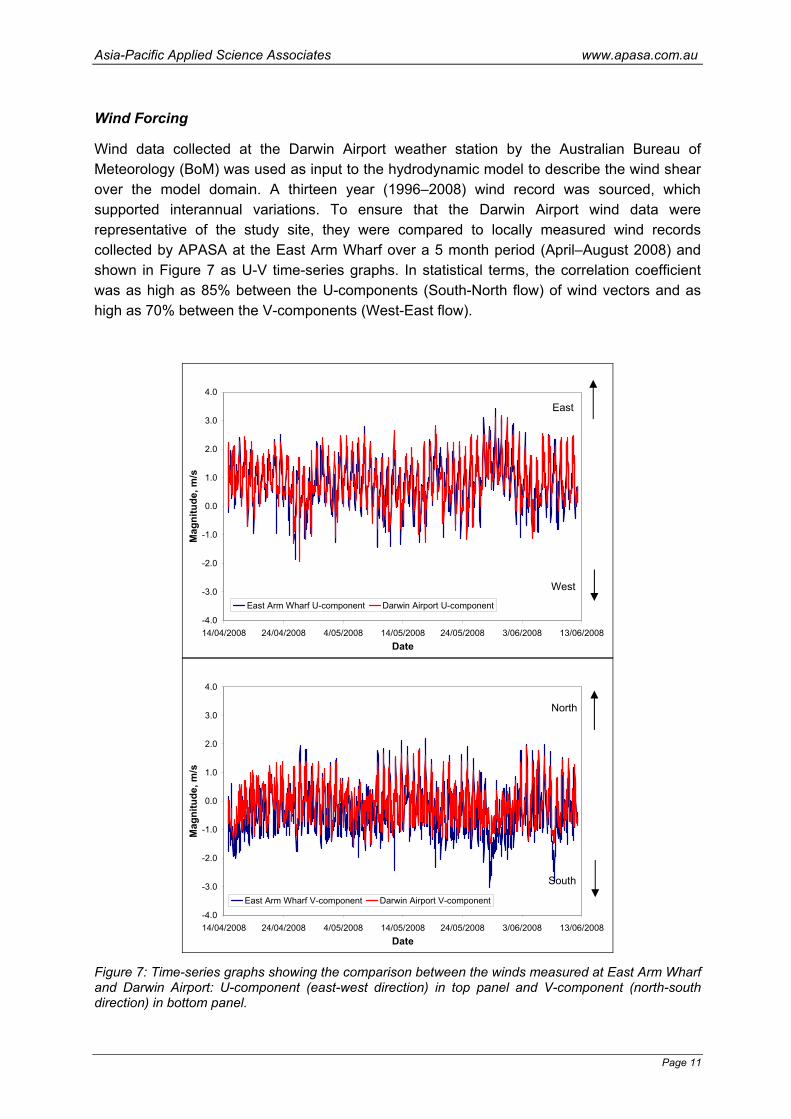
Wind Forcing

Wind data collected at the Darwin Airport weather station by the Australian Bureau of Meteorology (BoM) was used as input to the hydrodynamic model to describe the wind shear over the model domain. A thirteen year (1996–2008) wind record was sourced, which supported interannual variations. To ensure that the Darwin Airport wind data were representative of the study site, they were compared to locally measured wind records collected by APASA at the East Arm Wharf over a 5 month period (April–August 2008) and shown in Figure 7 as U-V time-series graphs. In statistical terms, the correlation coefficient was as high as 85% between the U-components (South-North flow) of wind vectors and as high as 70% between the V-components (West-East flow).

-4.0

-3.0

-2.0

-1.0

0.0

1.0

2.0

3.0

4.0

14/04/2008 24/04/2008 4/05/2008 14/05/2008 24/05/2008 3/06/2008 13/06/2008Date

Mag

nitu

de, m

/s

East Arm Wharf U-component Darwin Airport U-component

-4.0

-3.0

-2.0

-1.0

0.0

1.0

2.0

3.0

4.0

14/04/2008 24/04/2008 4/05/2008 14/05/2008 24/05/2008 3/06/2008 13/06/2008Date

Mag

nitu

de, m

/s

East Arm Wharf V-component Darwin Airport V-component

Figure 7: Time-series graphs showing the comparison between the winds measured at East Arm Wharf and Darwin Airport: U-component (east-west direction) in top panel and V-component (north-south direction) in bottom panel.

East

West

North

South


Page 12

Current validation

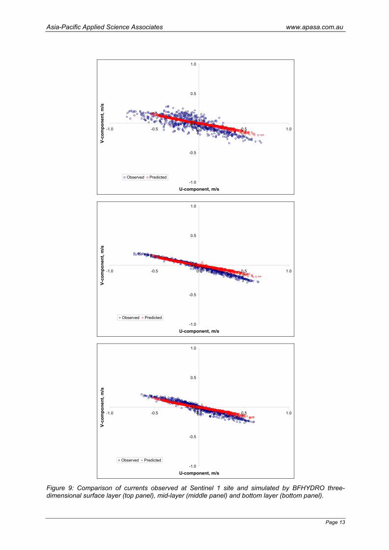
Measurements from 4 acoustic Doppler current-profilers (ADCPs) deployed in Darwin Harbour and Beagle Gulf (Figure 8) were used to compare the accuracy of the generated current data. All ADCPs were bottom mounted and measured the currents at vertical steps through the water column. Current velocity and directions were collected at 10 minute intervals. A detailed summary of the predicted and measured current data for all 4 ADCPs can be found in APASA (2009). The data comparisons from the Sentinel 1 deployment site, which was the closest to the wastewater release site, are included below for completeness.

Figure 9 shows the comparisons between the measured currents and the BFHYDRO model results. The currents are plotted as a scatter plot, hence, taking into consideration the current speed and velocities throughout the deployment period in the surface, middle and near-bottom water layers. As can be seen in Figure 9, the model predictions compared very well throughout the entire water column, in terms of both current speed and direction.

A statistical comparison between the measured and observed current speeds and directions also supported the validation of the model. The root mean square error in current speed was consistently low at all depths, remaining within the limits 0.12–0.14 m/s. The maximum deviations in predicted current directions were <10°. Therefore, the individual statistics confirmed that the model settings and formulations were capable of replicating the currents in the study area.

Figure 8: Locations of current and wind measurements used to validate current predictions.


Page 13

-1.0

-0.5

0.0

0.5

1.0

-1.0 -0.5 0.0 0.5 1.0

U-component, m/s

V-co

mpo

nent

, m/s

Observed Predicted

-1.0

-0.5

0.0

0.5

1.0

-1.0 -0.5 0.0 0.5 1.0

U-component, m/s

V-co

mpo

nent

, m/s

Observed Predicted

-1.0

-0.5

0.0

0.5

1.0

-1.0 -0.5 0.0 0.5 1.0

U-component, m/s

V-co

mpo

nent

, m/s

Observed Predicted

Figure 9: Comparison of currents observed at Sentinel 1 site and simulated by BFHYDRO three-dimensional surface layer (top panel), mid-layer (middle panel) and bottom layer (bottom panel).


Page 14

Current data at the proposed release site

To reflect the dredged channels for the proposed loading facility, the model bathymetric grid was modified (Figure 10) and model simulations were performed for 30 days of the dry season (July 2007) and 120 days of the wet season (January to April 2007). A longer dataset was generated for the wet season, because it was used as input into the far-field dispersion model that was required to run for at least 100 days.

Figure 10: Details of bathymetry amended to include the dredged region for the proposed jetty loading facility.

For comparative purposes the predicted near surface currents were extracted for a representative wet season month (January 2007) and a dry season month (July 2007) and plotted as current roses in Figure 11. The bottom panels show the predicted current speeds as a function of time for each month. The direction axis indicates the direction the current is heading towards.

From examination of the current roses, the most common directions were east-northeast and west-southwest, which is in line with the major flood and ebb tidal axis respectively. As indicated earlier, the wind shear upon the water surface had a negligible influence on steering of the currents. The current directions at the proposed release site are mainly steered by the coastlines.


Page 15

The predicted current speeds for the representative wet and dry months were similar, with magnitudes reaching up to 0.20 m/s and an average of 0.067 m/s.

Figure 11: Current roses for near surface currents (top panels) during wet and dry seasons and corresponding current speeds as a function of time (bottom panels).


Page 16

3 TREATED WASTEWATER PROPERTIES

The flow rates and composition of the treated wastewater are summarized in Table 1. The table shows that the temperature of discharge is comparative to the ambient waters, whilst the salinity levels would be significantly lower. Hence, the wastewater would be highly buoyant and would be expected to rise rapidly to the water surface. The release rate and TPH concentrations of the discharge are expected to be significantly lower during the dry season compared to the wet season. The flow rate will be higher during the wet season due to the heavy rainfalls experienced in the wet season. The TPH concentration will also be higher during the wet season because potentially oil contaminated runoff will be the primary source of TPH in the wastewater. Most of the all-season streams (that will flow during wet and dry seasons) will not contain any TPH; e.g. treated sewage.

Table 1: Summary of the wastewater characteristics for each season.

Input Wet season Dry season Wastewater Flow Rate (Continuous)

160 m3/hr 18 m3/hr

Salinity of wastewater 0.02 ppt 0.325 ppt

Temperature of wastewater 26 °C 35 °C

Total Petroleum Hydrocarbon concentration

10 mg/L 0.2 mg/L


Page 17

4 TPH-IN-HARBOUR WATER TRIGGER VALUE

Following an extensive literature search it was concluded that a trigger value of 0.007 mg/L (or 7 ppb) by Tsvetnenko (1998) would be appropriate for a conservative approach. Fandry (2003) also came to this conclusion during a review process for contaminants on the North West Shelf. Assuming a background value of zero and ignoring natural decay, for a 0.2 mg/L and 10 mg/L discharge, a dilution greater than 1:29 and 1:1428, respectively, would be required.


Page 18

5 NEAR FIELD MODELLING

Model Description

The near-field mixing of the treated wastewater was predicted using the fully three-dimensional flow model, Updated Merge (UM3) model. UM3 is a plume model for simulating single and multi-port submerged discharges, available in the US Environmental Protection Agency interface Visual Plumes (VP) (Frick et al., 2000). The UM3 model was selected since it has been extensively tested for various discharges and found to predict the observed dilutions more accurately (Roberts and Tian, 2004) than other near field models (e.g. RSB or CORMIX).

In this Lagrangian model, the equations for conservation of mass, momentum, and energy are solved at each time step, giving the dilution along the plume trajectory. To determine the growth of each element, UM3 uses the shear (or Taylor) entrainment hypothesis and the projected-area-entrainment hypothesis. The flows begin as round buoyant jets issuing from one side of the diffuser and can merge to a plane buoyant jet (Carvalho et al. 2001). Model output consists of plume characteristics, including centerline dilution, rise-rate, width, centreline height and diameter of the plume. Dilution is reported as the “effective dilution”, which is the ratio of the initial concentration to the concentration of the plume at a given point, following Baumgartner et al. (1994). The model includes corrections for a reduction in surface area that is available for mixing that occurs with merging plumes, created by discharge through multiple adjacent ports.

Ambient Environmental Conditions

The near-field modelling requires specification of typical ambient environmental conditions, including vertical density structure and background currents. The vertical density structure is defining for plume behaviour due to the importance of the relative (to the ambient waters) buoyancy of the diluting plume. The buoyancy dynamics in this case will be dominated by the temperature and salinity differences between the discharge and the ambient, or receiving, water.

Water quality sampling by URS revealed that the temperature and salinity structure at the site varies seasonally. The profiles showed a well mixed water column (negligible temperature and salinity variation) during a representative dry season month of July 2008.

The salinity and temperature profile data during a wet season month showed a stratified water body. The surface and bottom temperatures were found to vary by 3 °C, while the salinity varied by ~ 3 parts per thousand. This is likely due to the runoff of freshwater from nearby catchments during the heavy rainfall events. Table 2 exhibits the surface and bottom temperatures and salinities used as inputs into the near-field model.

Ambient currents were assessed as a depth average from the previously developed current dataset. Table 3 presents the 5th, 50th and 95th percentiles of current velocities. The 5th percentile of current velocity of 0.005 m/s was extracted to gain an understanding of the


Page 19

minimum current speed that would be exceeded 95% of the time (US EPA 2006). The 95th percentile velocity of 0.146 m/s would be exceeded only 5% of the time.

These conditions reflect two contrasting cases:

a) 5th percentile current velocity: slow currents, low dilution and slow advection

b) 95th percentile current velocity: fast currents, high dilution and rapid advection to nearby areas.

The direction of the main current axis was assumed to be towards the west, which is typical for flood currents.

Table 2. Temperature and salinity used as input into the near field model

Wet Season Dry Season Water Depth

Temperature (°C) Salinity (ppt) Temperature (°C) Salinity (ppt)

Surface 32.7 26.3 24.8 35.3

Bottom 30.9 29.3 24.4 35.5

Table 3. Ambient current conditions

Statistic Current speed (m/s)

5th Percentile 0.005



Maximum 0.211

Diffuser design

The near-field modelling was used to assist INPEX with the selection process for the outfall configuration. INPEX specified that the outfall is to be located along the product loading jetty (12°30′36.37″S, 130°54′30.95″E), in approximately 14 m of water (LAT). In addition, the discharge is to take place above the seabed (~1 m), and the discharge to be directed upwards and outwards.

As such a diffuser with port openings approximately 1 m above the seabed, orientated north in a 30° angle relative to horizontal was tested. The port openings were faced northward so that the discharge is perpendicular with the main tidal axis and propelling the wastewater into deeper waters.

To reduce the potential for the ports to be fouled by marine growth, particularly during the lower flow periods, a minimum internal port diameter of 0.1 m was selected. A maximum port


Page 20

diameter of 0.2 m was also tested to ensure that the exit velocity provided a sufficient turbulent mixing zone.

The port spacing is a function of rising plume geometry and the spacing that keeps the buoyant rising plumes separate until they reach the surface. The port spacing l is given by:

l = 1/3 H

where H is the water depth.

Assuming a water depth of 14 m, the approximate port spacing is 4.7 m. To confirm the empirical calculation, initial dilutions were tested for port spacings from 2 m to 10 m.

Table 4 gives a summary of the various diffuser parameters that were tested as part of the selection process.

Table 4. Summary of the outfall configurations examined as part of the near-field modelling

Port internal diameter tested (m) 0.1, 0.2

Angle of port orientation from horizontal (degrees) 30

Number of open ports tested 3, 4, 5, 6

Port spacings tested (m) 2, 3, 4, 5, 6, 8, 10

Water depth (depth to sea bottom below LAT once dredged) (m) 14

Height of port above seabed (m) 1

Direction of ports North

Sensitivity testing

The wet season settings were used to simulate and compare the near-field rate of dilution for each diffuser configuration. This involved testing of port spacing, number of ports and port diameters.

A simple outlet pipe was not considered due to the common notion that a multiport diffuser will achieve a greater initial dilution. A 2-port diffuser was not modelled because the exit velocity during the wet season conditions would be too high maintaining the shape of the jet throughout the water column without any essential dilution.

Figure 12 shows the near-field dilution as a function of port spacing for 4 ports with a 0.1 m port diameter. The results show that based on the empirical expression above, the 5 m port spacing gives an adequate dilution of 1:104, during the average static current (0.062 m/s). Doubling the spacing between the ports from 5 m to 10 m would increase the rate of dilution by 20% (1:126).


Page 21

Having established the port spacing, the next stage involved testing the number of ports. Figure 13 demonstrates that a four port configuration provided sufficient dilution, and that an increase of the number of ports to 5 and 6 did not significantly reduced the plume exit velocity and thus the dilution rate.

Figure 12. Near-field dilution comparison as function of static average current speed, 4 ports, 0.1 m port diameter, varying spacing during wet conditions

Figure 13. Near-field dilution results comparison as function of static average current speed, varying ports, 0.1 m port diameter, 5 m spacing during wet conditions


Page 22

The next step involved comparing the predicted dilutions of 0.1 m and 0.2 m port diameters under a range of static current speeds (Figure 14). Figure 14 clearly shows that the 0.1 m port diameter achieved a greater rate of dilution for the range of current speeds, which is primarily due to a higher exit velocity (~2.8 m/s for the 0.1 m port and 0.7 m/s for the 0.2 m port) near the port orifice.

Figure 14. Comparison of the near-field dilutions for a 0.1 m and 0.2 m port diameters, four ports, 5 m spacing, under a range of static current speeds at the proposed jetty during the wet season

Based on the near-field modelling comparison study, it was concluded that a diffuser with 4 ports, 0.1 m diameter and 5 m spacing would provide an adequate dilution.

Near-Field Results

The selected diffuser configuration was used as input into the UM3 model to predict the dispersion of the initial plume for the dry season and wet season scenarios.

In general, due to the exit velocity, the plume was initially driven by its own momentum horizontally from the outlet. As the plume velocity decreased (less than 1 m from the orifice), the buoyancy of the plume caused it to rise rapidly towards the water surface. Consequently, the velocity shear between the buoyant jet and their surroundings caused turbulence, which entrained the receiving water. Upon reaching the water surface it would remain at the sea


Page 23

surface and advect and disperse with the prevailing currents. Table 5 shows a summary of the plume characteristics for a range of static current speeds and scenario.

During a static weak current an initial dilution of 1:334 was achieved for the dry season scenario within 4 m from the diffuser. For the wet season case, dilutions of 1:76 were predicted within 11 m.

The trigger value of 0.007 mg/L would only be met by the dry season scenario within the near-field (Figure 15) since a low rate of dilution (1:29) was required and easily achieved. For the two wet season scenarios (Figure 16), the findings demonstrated that the rate of dilution was insufficient, and therefore a far-field modelling and analysis would be required to assess the extent of the mixing zone.

Table 5. Summary of the final near field modelling results for a 4 port, 5 m spacing 0.1 m diameter diffuser configuration.

Season Discharge rate (m3/hr)

TPH initial conc

(mg/L)

Plume Diameter

(m)

Final Salinity

(ppt)

Final Temp (°C)

TPH final conc

(mg/L) Dilution

Maximum Horizontal

Distance (m)

3.9 35.3 24.6 0.0005 334 2

8.7 35.4 24.5 0.0002 803 12 Dry 18 0.2

4.1 35.4 24.4 0.0002 807 18

11.4 27.8 31.5 0.1300 76 5

11.8 28.2 31.4 0.0879 112 9 Wet 160 10

10.7 28.5 31.3 0.0432 227 19


Page 24

Figure 15: Dry season case (18 m3/hr flow rate, 0.2 mg/L TPH) - near-field initial dilution results as a function of static current speeds.

Figure 16: Wet season case (160 m3/hr, 10 mg/L TPH) - near-field initial dilution results as function of static current speeds.


Page 25

6 FAR-FIELD MODELLING

Background

Detailed far-field modelling was carried out to estimate the mixing and dispersion of the treated wastewater discharge using an advanced three-dimensional plume behaviour model, MUDMAP. MUDMAP simulated the wastewater discharge as a conservative tracer (no reaction or decay applied) into a time-varying current field with the initial dilution set by the near-field modelling described in Section 5.5. The modelling was used to predict the temporally and spatially varying concentrations of TPH within the wastewater plume. The main objective of the far-field modelling was to estimate the extent and shape of the mixing zones setup by the wastewater TPH under the wet season current conditions.

The far-field modelling augments the near-field work by allowing the time-varying nature of currents to be included, together with the potential for recirculation of the plume back to the discharge location. In the latter case near-field concentrations can be increased due to the discharge plume mixing with the remnant plume from an earlier time. As the dilutions can be relatively low in weak currents, this may be a potential source of episodic increases in TPH concentration in the nearby waters.

Scenarios

From the near-field modelling, it was concluded that far-field modelling would be required for the wet season scenario simulated as a continuous release over a 100-day period.

Modelling of the dry season was not required as the mixing within the near-field demonstrated that the necessary dilution would be achieved.

Far-Field Model

The three-dimensional plume behaviour model, MUDMAP, was used to simulate the wastewater mixing and dispersion. MUDMAP is an industry standard computerised modelling system, which has been applied throughout the world to predict the dispersion of sediment (cuttings and muds) and liquid (produced water) discharges since 1994 (Spaulding, 1994). The model is a development of the Offshore Operators Committee (OOC) model and like the OOC model calculates the fates of discharges through three known distinct integrated stages (Koh and Chang, 1973; Khondaker 1999). The stages are:

Stage 1: Convective descent/jet stage determines the initial dilution and spreading of the material in the immediate vicinity of the release location. This is calculated from the discharge velocity, momentum, entrainment and drag forces

Stage 2: Dynamic collapse stage determines the spread and dilution of the released material as it either hits the sea surface or sea bottom or becomes trapped by a strong density gradient in the water column. Advection, density differences and density gradients drive the transport of the plume; and

Stage 3: In Dispersion stage the model predicts the transport and dispersion of the discharged material by the local currents. Dispersion of the discharged material will be


Page 26

enhanced with increased current speeds and water depth and with greater variation in current direction over time and space.

Including these 3 stages as part of the predictions is necessary because the material will go through these distinct phases over different temporal and spatial scales. The governing equations and solution methodology in MUDMAP build on the formulation originally developed by Koh and Chang (1973) and extended by the work of Brandsma and Sauer (1983). The far-field calculation (passive dispersion stage), employs a particle-based, random walk procedure. The system has been extensively validated and applied for discharge operations in Australian waters (e.g. Burns et. al., 1999; King and McAllister, 1998, 1997).

The model predicts the dynamics of the discharge plume and resulting concentrations and plume thickness over the near-field (i.e. the immediate area of discharge) and far-field (wider region). The discharged material is represented by a large sample of Lagrangian particles. These particles are moved in three dimensions over each subsequent time step according to the current data and horizontal and vertical mixing coefficients.

Discharge Input Data

The detailed input data used in the discharge model setup included: • The relative temperatures, salinities and densities of the discharge and receiving

waters

• The rate of discharge of the wastewater

• The size and orientation of the discharge pipe

• The velocity of the discharge jet

• The height of the discharge point relative to mean sea level

• Current data to represent local physical forcing.

Table 6 presents a summary of the far-field model parameters used to simulate the wastewater discharge during the wet season. Evaporation and biodegradation were not parameterised and thus modelled; this makes the dilution estimates and resulting contours conservative.

Based on the near-field modelling results, a minimum dilution of 1:100 at a distance of 20 m was used to account for the jet plume and buoyancy dynamics adjacent to the release site. This involved releasing the plume within the near surface waters (~1 m) and selecting appropriate mixing coefficients.


Page 27

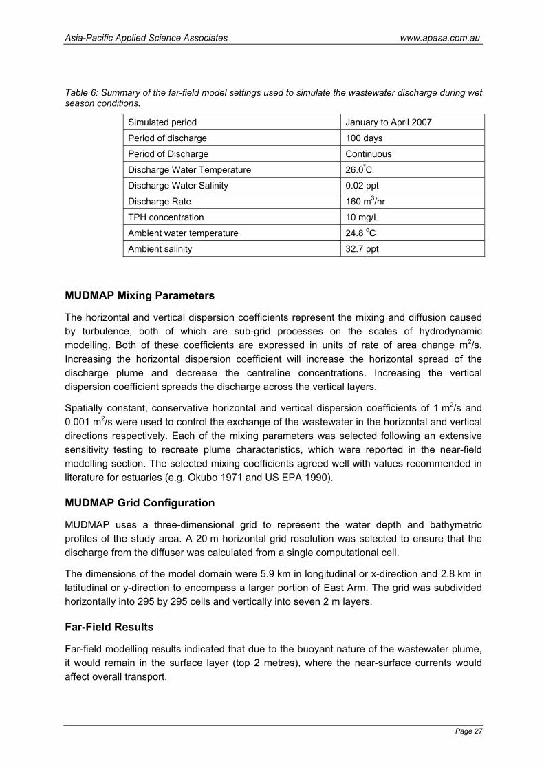
Table 6: Summary of the far-field model settings used to simulate the wastewater discharge during wet season conditions.

Simulated period January to April 2007

Period of discharge 100 days

Period of Discharge Continuous

Discharge Water Temperature 26.0ºC

Discharge Water Salinity 0.02 ppt

Discharge Rate 160 m3/hr

TPH concentration 10 mg/L

Ambient water temperature 24.8 oC

Ambient salinity 32.7 ppt

MUDMAP Mixing Parameters

The horizontal and vertical dispersion coefficients represent the mixing and diffusion caused by turbulence, both of which are sub-grid processes on the scales of hydrodynamic modelling. Both of these coefficients are expressed in units of rate of area change m2/s. Increasing the horizontal dispersion coefficient will increase the horizontal spread of the discharge plume and decrease the centreline concentrations. Increasing the vertical dispersion coefficient spreads the discharge across the vertical layers.

Spatially constant, conservative horizontal and vertical dispersion coefficients of 1 m2/s and 0.001 m2/s were used to control the exchange of the wastewater in the horizontal and vertical directions respectively. Each of the mixing parameters was selected following an extensive sensitivity testing to recreate plume characteristics, which were reported in the near-field modelling section. The selected mixing coefficients agreed well with values recommended in literature for estuaries (e.g. Okubo 1971 and US EPA 1990).

MUDMAP Grid Configuration

MUDMAP uses a three-dimensional grid to represent the water depth and bathymetric profiles of the study area. A 20 m horizontal grid resolution was selected to ensure that the discharge from the diffuser was calculated from a single computational cell.

The dimensions of the model domain were 5.9 km in longitudinal or x-direction and 2.8 km in latitudinal or y-direction to encompass a larger portion of East Arm. The grid was subdivided horizontally into 295 by 295 cells and vertically into seven 2 m layers.

Far-Field Results

Far-field modelling results indicated that due to the buoyant nature of the wastewater plume, it would remain in the surface layer (top 2 metres), where the near-surface currents would affect overall transport.


Page 28

Throughout the sample wet season currents (January to April 2007), the plume was predicted to oscilliate with the flood and ebb tides. The concentrations were found to be patchy within the plume that was caused by variations in the current flow above the outfall. The TPH concentrations were generally predicted to be low when tides were flooding or ebbing. However, patches of higher concentrations tended to build up at the turn of the tide. These patches moved as a cohesive unit as the current speeds increased again. Dispersion of these higher concentration patches tended to be present within the wider plume at any one time, sometimes combining when current reversals caused patches to move back and build up.

Episodes of “second dosing”, when the wastewater plume moved back at some later time due to the oscillatory nature of the tidal currents, also contributed to variability in spatial plume concentration. These findings are in agreement with the research of King and McAllister (1997, 1998) who also noted that concentrations of total oils within produced water plumes generated by Harriet Alpha platform were patchy and peak around the changing of the tides.

Figure 17 shows a sample time-series of the maximum predicted in-water TPH concentrations, during sample January 2007 current conditions. The results are based on a 160 m3/hr discharge of wastewater with 10 mg/L initial TPH concentration. The sample plots show a build up in concentration during the time of current reversal. This patch of higher concentration was then transported away from the release site as current speed increased.

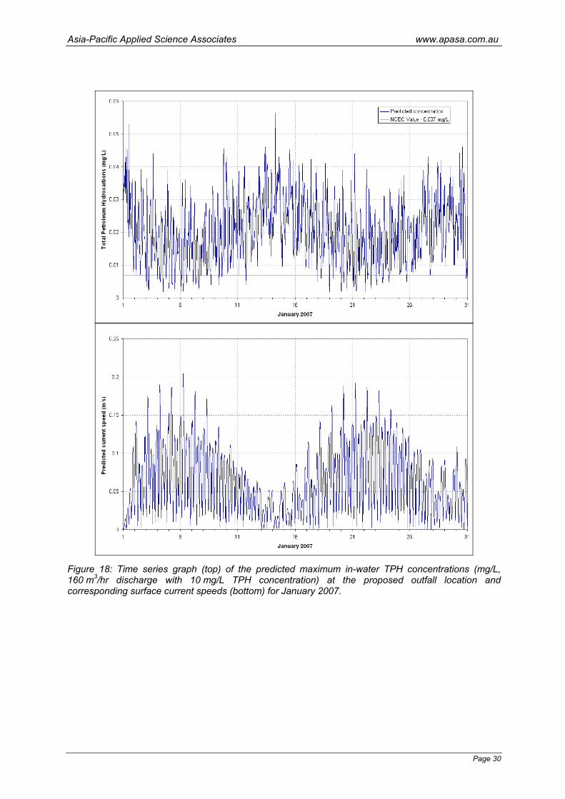
Figure 18 shows a sample time-series graph of the predicted TPH concentrations within the outfall cell point. The graph highlights that the concentrations in the initial mixing zone (within 20 m of the discharge) would vary over time with the tidal cycle and episodes of stronger and weaker currents. This is emphasized by the bottom graph which shows the predicted surface currents for the corresponding period.

Figure 19 shows the predicted fluctuations of TPH maximum in-water concentrations for sites at 100m, 200m and 300 m west from the release site. As each of the graphs show, concentrations significantly decreased as a function of distance from the source. By 300 m the maximum concentration had reduced to 0.01 mg/L.


Page 29

(a) 6 pm 14th January 2007 (d) 12 am 15th January 2007

(b) 8 pm 14th January 2007 (e) 2 am 15th January 2007

(c) 10 pm 14th January 2007 (f) 4 am 15th January 2007

Figure 17: Example time series of the maximum predicted in-water TPH concentrations (mg/L, 160 m3/hr discharge with 10 mg/L TPH concentration), January 2007 current conditions


Page 30

Figure 18: Time series graph (top) of the predicted maximum in-water TPH concentrations (mg/L, 160 m3/hr discharge with 10 mg/L TPH concentration) at the proposed outfall location and corresponding surface current speeds (bottom) for January 2007.


Page 31

Figure 19: Time series graphs of the predicted maximum in-water TPH concentrations (mg/L) at 100 m (top), 200 m (middle) and 300 m (bottom) west of the release site


Page 32

To reinforce this conclusion and to determine the zone of effect, the 50th and 95th percentile concentration contours were calculated using the 100-day simulation results (Figure 20). Both statistics were selected to represent likely TPH for 50% and 95% of the time for the examined continuous flow rates and concentrations.

There was a general trend for the TPH concentrations to form an elliptical shape in the westerly and easterly direction, in line with the major tidal axis. The 50th and 95th percentile contour extents were almost identical for both these scenarios, which is logical given the flow rate and initial concentration ratios were the same.

Table 7 shows the predicted area of coverage and maximum distance from the release site for each of the percentiles as function of concentration. The results show that the TPH concentration of trigger value of 0.007 mg/L was within 86 m from the release site for the 50th percentile and 330 m for the 95th percentile. The 0.007 mg/L contour was predicted to encircle a surface area of 14 051 m2 for the 50th percentile analysis, compared to 114 055 m2 for the 95th percentile. For the 95th percentile (the limit that encompasses 95% of all occurrences), the 0.007 mg/L TPH contour was found to be approximately 440 m from the nearest coastline.

Table 7: Predicted area of coverage and maximum distance for the 50th and 95th percentile concentrations.

Percentile statistic Concentrations greater than

Maximum Distance from the release site (m)

Area of coverage (hectares)

0.007 mg/L 86 1.4

0.010 mg/L 58 0.7 50th

0.015 mg/L 27 0.2

0.007 mg/L 330 11.4

0.010 mg/L 196 5.3 95th

0.015 mg/L 105 1.9


Page 33

Figure 20: Predicted 50th (top); and 95th (bottom) percentiles of TPH concentrations (mg/L, 160 m3/hr discharge with 10 mg/L TPH concentration), January to April 2007 current conditions


Page 34

7 CONCLUSIONS AND RECOMMENDATIONS

A dispersion modeling study was carried out to simulate the discharge of treated wastewater as part of the INPEX onshore processing facility. The main objectives of the study were to address the following:

• Assist in the selection of a diffuser configuration that will ensure sufficient dilution at the proposed discharge point to minimise impacts on nearby marine habitats; and

• Estimate the extent of the active mixing zone during both wet and dry season conditions.

Based on an extensive near-field modelling assessment, it was concluded that a diffuser with 4 ports, 0.1 m diameter and 5 m spacing would provide an adequate dilution.

An extensive literature search identified a trigger value of 0.007 mg/L (or 7 ppb) by Tsvetnenko (1998) would be appropriate for a conservative approach. Fandry (2003) also came to this conclusion during a review process for contaminants on the North West Shelf for the CSIRO. Using the diffuser configuration selected and ambient conditions, it was found that the dry season scenario would meet the TPH requirement of 0.007 mg/L within the near-field but that far-field analysis would need to be undertaken to assess the extent of the required mixing zone to satisfy the chemical 0.007 mg/l criteria for the wet season scenario.

Far-field results indicated that the plume would oscilliate with each flood and ebb tide, consecutively the concentrations would be patchy and variable. Lowest concentrations were predicted to occur during stronger currents. However, patches of higher concentrations tended to build up at the turn of the tide (slack tides). These patches moved as a cohesive unit as the current speeds increased again.

Fiftieth and ninety-fifth percentile concentration contours were calculated using the 100-day simulations, to define the zone of effect for the wet season scenario. There was a general trend for the TPH concentrations to form an elliptical shape in the westerly and easterly direction, in line with the major tidal axis. Both 50th and 95th percentile contour extents were very similar.

The TPH concentration of trigger value of 0.007 mg/L was within 86 m from the release site for the 50th percentile and 330 m for the 95th percentile. The predicted area of coverage was 1.4 and 11.4 hectares for the 50th and 95th percentiles, respectively. Finally, for the 95th percentile (the limit that encompasses 95% of all occurrences), the 0.007 mg/L TPH contour was found to be approximately 440 m from the nearest coastline.

Finally, given that the far-field modelling was carried out as a continuous 100-day release it would be considered as “worst case” results, given that rain fall durations would be shorter.


Page 35

8 REFERENCES

Baumgartner, D., Frick, W. and Roberts, P. 1994. Dilution models for Effluent Discharges. 3rd Ed. EPA/600/R-94/086. U.S. Environment Protection Agency, Pacific Ecosystems Branch, Newport, Oregon.

Brandsma, M.G. and Sauer, T. C. Jr. 1983. The OOC model: prediction of short term fate of drilling mud in the ocean, Part I model description and Part II model results. Proceedings of Workshop on An Evaluation of Effluent Dispersion and Fate Models for OCS Platforms. Santa Barbara, California, 7-10 February, 1983.

Burns, K., Codi, S., Furnas, M., Heggie, D., Holdway, D., King, B. and McAllister, F. 1999. Dispersion and Fate of Produced Formation Water Constituents in an Australian Northwest Shelf Shallow Water Ecosystem. Marine Pollution Bulletin 38, No. 7: 593 – 603.

Fandry, C. 2003. North West Shelf Joint Environmental Management Study. Containment on the North West Shelf: sources, impacts, pathways and effects. CSIRO Technical Report.

Falconer, R. A. and Chen, Y. 1991. An improved representation of flooding and drying and wind stress effects in a two-dimensional tidal numerical model. Proc. Instn Civ. Engrs, Part 2: 659-678.

Frick, W.E.1984. Non-empirical closure of the plume equations. Atmospheric Environment 18, No. 4: 653-662.

Frick, W.E., Roberts, P.J.W., Davis, L.R., Keyes, J., Baumgartner, D.J. and George, K.P. 2003. Dilution Models for Effluent Discharges (Visual Plumes). 4th Ed, Ecosystems Research Division, NERL, ORD, USEPA.

Huang, W. and Spaulding, M.L. 1995. A three dimensional numerical model of estuarine circulation and water quality induced by surface discharges. ASCE Journal of Hydraulic Engineering 121 No. 4, April 1995: 300-311.

King, B. and McAllister, F.A. 1997. Modeling the Dispersion of Produced Water Discharge in Australia 1 & 2. Australian Institute of Marine Science report to the APPEA and ERDC.

King, B. and McAllister, F.A. 1998. Modelling the dispersion of produced water discharges. APPEA Journal: 681-691.

Koh, R.C.Y. and Chang, Y.C. 1973. Mathematical model for barged ocean disposal of waste. Environmental Protection Technology Series EPA 660/2-73-029, U.S. Army Engineer Waterways Experiment Station. Vicksburg, Mississippi.

Khondaker, A. N. 2000. Modeling the fate of drilling waste in marine environment – an overview. Journal of Computers and Geosciences 26: 531-540.

Mathison, J.P., Jenssen, O.O., Utnes, T., Swanson, J.C. and Spaulding, M.L. 1989. A Three Dimensional Boundary Fitted Coordinate Hydrodynamic Model, Part II: Testing and Application of the Model. Dt. hydrog, Z.42: 188-213.

Mendelsohn, D., Peene, S., Yassuda, E., Davie, S. 1999. A hydrodynamic model calibration study of the Savannah River Estuary with an examination of factors affecting salinity


Page 36

intrusion. Proceedings from Estuarine and Coastal Modelling 6 (ECM6). New Orleans, LA, 3-5 November 1999.

Muin, M. and Spaulding, M.L. 1997. A three dimensional boundary fitted coordinate hydrodynamic model. Journal of Hydraulic Engineering 123 No. 1, January 1997: 2-12.

Okubo, 1971. Oceanic diffusion diagrams. Deep-Sea Research 8: 789–802.

Roberts, P. and Tian, X. 2004. New experimental techniques for validation of marine discharge models. Environmental Modelling and Software 19: 691-699.

Sankaranarayanan. S., and Ward, M.C. 2006. Development and application of a three-dimesional orthogonal coordinate semi-implicit hydrodynamic model. Journal of Continental Shelf Research 26.

Spaulding, M., Mendelsohn, D., and Swanson, J.C. 1999. WQMAP: An integrated three-dimensional hydrodynamic and water quality model system for estuarine and coastal applications. Marine Technology Society Journal 33 No. 3, Fall 1999: 38-54.

Swanson, J. C. 1986. A three-dimensional numerical model system of coastal circulation and water quality. PhD dissertation, University of Rode Island, Kingston, R. I.

Tsvetnenko, Y. 1998. Derviation of Australian tropical marine water quality criteria for the protection of aquatic life from adverse effects of petroleum hydrocarbons. Journal of environmental toxicology and water quality 13 No. 4: 273 -284.

US EPA., 2006. Technical Evaluation: Physical Characteristics of Discharge. US EPA document, 40 CFR 125.62 (a).

Yassuda, E., Davie, S., Mendelsohn, D., Isaji, T., and Peene, S. 1999. Development of a waste load allocation model within Charleston Harbor estuary phase II: water quality. Estuary. Coastal and Shelf Science 50: 1571–1594.

Zigic, S. 2005a. Methodology to calculate the time-varying flow through a hydraulic structure connecting two water bodies. PhD Dissertation. Griffith University, Gold Coast.

Zigic, S., King, B. and Lemckert, C. J. 2005b. Modelling the two-dimensional flow between an estuary and lake connected by a bi-directional hydraulic structure. Estuarine, Coastal and Shelf Science 63: 33 -41.

Documents

Appendix 10 - NTEPA · Appendix 10 Wastewater discharge modelling. ICHTHYS GAS FIELD DEVELOPMENT PROJECT WASTEWATER DISCHARGE MODELLING Prepared for INPEX Browse, Ltd. May 2009 INPEX