Embed Size (px)
Citation preview

AppendicesAppendix ATransmission Lines
Power system’s main power corridor: Transmission lines and transformers with atwo-port network.
Referring to Fig. A.1a approximated two port transmission network and(b) phasor diagram:
V receiving end phase voltageE sending end phase voltageP single-phase real powerQ single-phase reactive power
BCj j ¼ XIcosu ¼ E sind
Hence Icosu ¼ EX sind
ACj j ¼ XIsinu ¼ Ecosd� V
Hence Isinu ¼ EX cosd� V
XReal power, P ¼ VIcosu ¼ EV
X sind
) P dð Þ ¼ EVX
sind power-angle characteristics
d is known as the load angle or power angle
Since the real power P depends on the product of phase voltages and the sine ofthe angle d between their phasors. In power networks, node voltages must be withina small percentage of their nominal values. Hence such small variations cannotinfluence the value of real power. Large changes of real power, from negative topositive values, correspond to changes in the sin d. The system can operate only inthat part of the characteristic which is shown by a solid line in Fig. A.1c. The angle
© Springer Nature Singapore Pte Ltd. 2018T. Bambaravanage et al., Modeling, Simulation, and Control of a Medium-ScalePower System, Power Systems, https://doi.org/10.1007/978-981-10-4910-1
159

d is strongly connected with system frequency f; hence the pair ‘P and f’ is alsostrongly interrelated.
Reactive power,
Q ¼ EVX
cos d� V2
X
cos d ¼ffiffiffiffiffiffiffiffiffiffiffiffiffiffiffiffiffiffiffi1� sin2 d
p
Q ¼ffiffiffiffiffiffiffiffiffiffiffiffiffiffiffiffiffiffiffiffiffiffiffiffiEVX
� �2
�P2
s
� V2
X
Due to stability considerations, the system can operate only in that part of thecharacteristic which is shown by a solid line. The smaller the reactance X, thesteeper the parabola; even for small changes in V, cause large changes in reactive
(a)
(b)
(c)
Fig. A.1 a Two-port p equivalent circuit corresponding to an approximated transmission line.b Corresponding phasor diagram. c Real power and reactive power characteristics
160 Appendix A: Transmission Lines

power. Obviously the inverse relationship also takes place: a change in reactivepower causes a change in voltage.
Hence the three factors that can affect the stability of PS can be identified as:
• Load angle, d• Frequency, f• Nodal voltage magnitude, V
Appendix A: Transmission Lines 161

Appendix BComposite Loads
Usually each composite load represents a relatively large fragment of the systemtypically comprising
• low- and medium-voltage distribution networks,• small power sources operating at distribution levels,• reactive power compensators,• distribution voltage regulators,• a large number of different component loads such as motors, lighting and
electrical appliances [6].
In the steady state the demand of the composite load depends on the bus-barvoltage V and the system frequency f. The functions describing the dependence ofthe active and reactive load demand on the voltage and frequency P(V, f) and Q(V,f) are called the static load characteristics.
The characteristics P(V) and Q(V), taken at constant frequency, are called thevoltage characteristics while the characteristics P(f) and Q(f), taken at constantvoltage, are called the frequency characteristics. The slope of the voltage or fre-quency characteristic is referred to as the voltage (or frequency) sensitivity of theload. Figure B.1, illustrates this concept with respect to voltage sensitivities.
Voltage sensitivities kPV and kQV and the frequency sensitivities kPF and kQF areusually expressed in per units with respect to a given operating point:
kPV ¼ DP=P0
DV=V0
kQV ¼ DQ=Q0
DV=V0
kPf ¼ DP=P0
Df =f0
© Springer Nature Singapore Pte Ltd. 2018T. Bambaravanage et al., Modeling, Simulation, and Control of a Medium-ScalePower System, Power Systems, https://doi.org/10.1007/978-981-10-4910-1
163

kQf ¼ DQ=QP0
Df =f0
where,P0, Q0, V0, f0, DP and DQ, are: real power, reactive power, voltage, frequency,
real power change, and reactive power change at a given operating point.A load is considered to be stiff, if at a given operating point, its voltage sensi-
tivities are small.If,
• kPV ’ 0kQV ’ 0, the load is considered to be ideally stiff. The power demand of thatload does not depend on the voltage.
• A load is voltage sensitive if kPV and kQV are high• For a small DV change cause high change in the demand, DP .• Usually kPV\kQV
Fig. B.1 Illustration of thedefinition of voltagesensitivity
164 Appendix B: Composite Loads

Appendix CGeneration Characteristic
In the steady state, the idealized power–speed characteristic of an ith generating unitcan be written as:
Dxxn¼ �qDPm
Pn
DPm
Pn¼ �K Dx
xn
Dffn¼ �qi
DPmi
Pni
DPmi
Pni¼ �Ki
Dffn
In the steady state, all the generating units operate synchronously at the samefrequency. When,
Dx fraction of rated speedxn rated speedx turbine speedDf fraction of frequencyf system frequencyDPT the overall change in the total power generatedNG no. of generator unitsPm turbine powerPn nominal power output;
DPT ¼XNG
i¼1DPmi
�KiDffn¼ DPmi
Pni
© Springer Nature Singapore Pte Ltd. 2018T. Bambaravanage et al., Modeling, Simulation, and Control of a Medium-ScalePower System, Power Systems, https://doi.org/10.1007/978-981-10-4910-1
165

)DPT ¼ �Dffn
XNG
i¼1KiPni
) DPT ¼ �DfXNG
i¼1
KiPnifn
� �ðC:1Þ
Figure C.1, illustrates how the characteristics of individual generating units canbe added according to Eq. (C.1) to obtain the equivalent generation characteristic.This characteristic defines the ability of the system to compensate for a powerimbalance at a situation of a system frequency deviation from its rated value. For apower system with a large number of generating units, the generation characteristicis almost horizontal such that even a relatively large power change only results in avery small frequency deviation. This is one of the benefits due to combininggenerating units into one large system.
To obtain the equivalent generation characteristic of Fig. C.2, it has beenassumed that the speed–droop characteristics of the individual turbine-generatorunits are linear over the full range of power and frequency variations. In practice theoutput power of each turbine is limited by its technical parameters. The speed–droop characteristics of a turbine with an upper limit is shown in Fig. C.2.
If a turbine is operating at its upper power limit then a decrease in the systemfrequency will not produce a corresponding increase in its power output. At thelimit q = ∞ or K = 0 and the turbine does not contribute to the equivalent systemcharacteristic. Consequently the generation characteristic of the system will bedependent on the number of units operating away from their limit at part load; thatis, it will depend on the spinning reserve, where the spinning reserve is thedifference between the sum of the power ratings of all the operating units andtheir actual load.
Fig. C.1 Generation characteristic as the sum of speed–droop characteristics of all the generationunits
166 Appendix C: Generation Characteristic

The allocation of spinning reserve is an important factor in power systemoperation as it determines the shape of the generation characteristic. This isdemonstrated in Fig. C.3, with two generating units.
In Fig. C.3a, the spinning reserve is allocated proportionally to both units (whichoperate at a frequency off0) and the maximum power of both generators is reachedat the same operating frequencyf1. The sum of both characteristics is then a straightline (as given in Eq. (C.1)), up to the maximum powerPMAX ¼ PMAX1þ PMAX2.
Figure C.3b shows a situation where the total system reserve is the same (equalto the amount of the previous case), but it is allocated solely to the second gen-erator. That generator is loaded up to its maximum at the operating point (fre-quencyf2). The resulting total generation characteristic is nonlinear and consists oftwo lines of different slopes. The first line is formed by adding both inverse droops,KT1 6¼ 0 and KT2 6¼ 0, in Eq. (C.3). The second line is formed noting that the firstgenerator operates at maximum load and KT1= 0, so that only KT2 6¼0 appears in thesum in Eq. (C.3). Hence the slope of that characteristic is higher (Fig. C.3).
Generally, the number of units operating in a real system is large. Some of themare loaded to the maximum but others are partly loaded, generally in a non-uniformway, to maintain a spinning reserve. Adding up all the individual characteristicswould give a nonlinear resulting characteristic consisting of short segments withincreasingly steeper slopes. That characteristic can be approximated by a curve asshown in Fig. C.4. The higher the system load, the higher the droop until itbecomes infinite qT = ∞, and its inverse KT = 0, when the maximum power PMAX
is reached. If the dependence of a power station’s auxiliary requirements on fre-quency were neglected, that part of the characteristic would be vertical (shown as adashed line in Fig. C.4).
The total system power generation is equal to the total system load (PL),including transmission losses.
XNG
i¼1Pmi ¼ PL
Fig. C.2 Speed–droop char-acteristic of a turbine with anupper limit
Appendix C: Generation Characteristic 167

Equation (C.1)/PL gives:
DPT
PL¼ �KT
Dffn
orDffn¼ �qT
DPT
PLðC:2Þ
(a)
(b)
Fig. C.3 Influence of the turbine upper power limit and the spinning reserve allocation on thegeneration characteristic
Fig. C.4 Static system gen-eration characteristic
168 Appendix C: Generation Characteristic
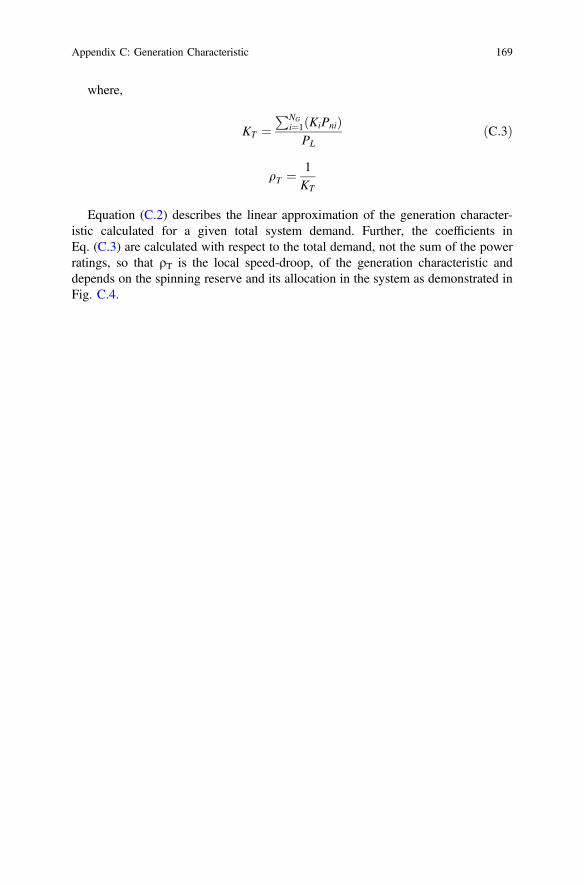
where,
KT ¼PNG
i¼1 KiPnið ÞPL
ðC:3Þ
qT ¼1KT
Equation (C.2) describes the linear approximation of the generation character-istic calculated for a given total system demand. Further, the coefficients inEq. (C.3) are calculated with respect to the total demand, not the sum of the powerratings, so that qT is the local speed-droop, of the generation characteristic anddepends on the spinning reserve and its allocation in the system as demonstrated inFig. C.4.
Appendix C: Generation Characteristic 169

Appendix D
Generation and transmission network of Sri Lanka as at 2011.
1130
PO
LPI-
1
132.
9
1170
SA
MA
N-1
134.
6
1210
BO
WA
T-1
131.
4
1770
KIR
IB-1
2220
KO
TMA
-2
224.
8
2230
VIC
TO-2
226.
8
2240
RA
ND
E-2
227.
3
2250
RA
NTE
-2
227.
3
32.9
32.8
3620
BA
DU
L-3
33.4
12.6
4252
RA
NTE
-G2
1790
RA
TMA
-1
130.
8
1300
KE
LAN
-1
130.
9
130.
8
4760
CO
L_F
-11
11.0
4750
CO
L_E
-11
129.
7
3500
KO
SG
A-3
33.3
33.3
3670
MA
TAR
A-3
133.
3
33.1
133.
4
3520
NU
WA
R-3
33.3
1520
NU
WA
R-1
132.
3
1620
BA
DU
L-1
131.
8
3540
OR
UW
A-3
32.7
1670
MA
TAR
A-1
132.
6
130.
5
1660
EM
BIL
-1
1100
LAX
-1
133.
3
130.
4
3200
UK
UW
E-3
3530
THU
LH-3
33.2
33.1
2300
KE
LAN
-2
217.
4
1540
OR
UW
A-1
130.
6
1530
THU
LH-1
130.
2
133.
7
217.
1
33.0
3860
MA
DA
M-3
133.
8
221.
2
1705
NE
WA
NU
-1
133.
2
1700
AN
UR
A-1
1850
PA
NA
D-1
127.
8
1800
MA
TUG
-1
129.
8
130.
4
1240
VA
VU
N-1
3240
VA
VU
N-3
3
33.3
33.1
32.8
134.
5
3400
HA
MB
A-3
3
32.5
3660
EM
BIL
-3
33.1
32.8
33.1
1160
ING
IN-1
127.
2
3160
ING
IN-3
125.
7
33.3
3700
AN
UR
A-3
A
217.
4
33.1
33.3
1710
TRIN
C-1
33.1
130.
6
32.9
33.0
134.
4
33.1
3690
HA
BA
R-3
33.1
1740
RA
TNA
P-1
133.
533
.0
1595
KH
D -
1
132.
4
132.
0
1600
BO
LAW
-1
131.
633
.4
132.
8
33.3
1840
JPU
RA
_1
130.
513
0.4
129.
9
129.
8
11.0
4435
CO
L_A
_11
3890
DE
HIW
_3
33.2
3800
MA
TUG
-3
33.2
134.
6
33.3
12.
0
0.8
12.
0
0.8
29.4
5.1 29.4
5.1
28.9 3.6
28.9 3.6
11.2
8.0
11.2
8.0
29.7
2.7
29.4
4.5
4.1 4.5
4.1
10.4
1.5
49.5
3.0
1.0
2.8
36.2
19.0
12.3
39.0
25.1
15.0
10.5
30.0
13.6
1.6
7.2
1.6
7.2
7.5
2.7 7.5
2.7
18.0
29.7
29.4
1.8
5.9
8.0
21.1
19.1 3.9
19.1 3.9
19.4
5.1
19.
2
7.3
28.8
11.2 28.8
17.0
72.8
38.4
47.
0
24.
347
.0
24.3
60.5
35.0
60.
5
5.9
8.0
12.0
11.0
14.0
4.3
0.6
10.8 0.6
10.8
0.0
0.0
0.0
0.0
81.9
77.2
81.2
85.7
81.9
77.2
81.2
85.7
7.1
1.5
7.1
1.5
17.3
0.3
17.
2
2.0
59.
1
44.
7
59.
1
44.
7
19.9
14.8
14.8
2.0
0.3
1.8
24.
8
20.
7 2
4.8
20.
7
49.5
41.3
11.0
3.6
3.3
1.0
0.0
0.0
0.0
5.2
0.0
0.0
6.9
14.
16.
9
14.
1
0.0
0.5
0.0 0.0
81.4
79.9
10.
911
.0
11.6
3.0
5.2
9.0
1.7
3.0
5.2
24.0
16.1
25.2
13.340.0
125.4
51.7
125.9
125.4
51.7
125.9
54.1
32.2
4.3
21.
6
21.
6
9.8
18.8
12.0
18.7
13.0
0.1
0.9
0.1
0.9
0.2
6.1
89.
0
63.
8
89.3
89.
0
63.
8
89.3
63.3
63.0
0.0
0.0
46.
0
42.
1
26.0
12.0
25.
7
12.
926
.0
12.0
51.0
35.6
12.7
129.
6
47.8
129
.2
46.
312
9.6
47.8
129
.2
46.
3
97.6
23.7
97.6
23.7
21.1
28.
0
12.
0 2
8.0
12.
0
6.5
22.8
16.4
28.
6
49.3
34.5
28.6
8.3
28.
6
0.0
10.1
0.0
78.0
36.7
117.
1
58.2
25.9
26.0
13.9 1
2.0
1.1
9.2
9.3
1.6
18.4
6.6
33.9
7.4
33.0
28.0
6.0
18.
6
5.6
18.7
3.6
37.0
14.5
18.5
7.3
18.5
7.3
1.0000
49.5
2.4
30.3
30.2
32.4
5.8
17.3
0.6
17.3
0.6
3.3
8.6
5.3 8.6
5.3
47.2
35.2
47.2
37.2
47.2
35.2
47.2
37.2 97.5
5.5
5.5
2.5
3.7
4.5
11.
7
1 27.1
12.4R
32.3
17.0H
1
40.0
2.5R
1
2.0
1
2.7
1 38.0
13.0
1
1
15.0
2.9R
1
38.0
17.4
1
46.0
36.0
1 15.0
10.0
1 39.0
22.0
1 15.0
5.0
1 18.0
7.0
1
1
51.0
1
11.0
4.4
1
14.0
1
0.0
1
30.0
12.0
2.0
0.3
1
49.5
37.1
1
1 0.0
0.0
1 36.2
19.0
1 45.8
1 11.0
3.2
SW
0.0
1 3.3
1
0.0
1
18.4
6.1
27.1
12.4R
2 32.0
2
40.0
2.5R
28.5
3.0
L
2
22.5
2.0
L
1
25.0
0.0L
1
11.0
48.0
20.0
H
2
1
20.0
10.0
H
2
1
47.0
30.0
SW
9.9
1 24.0
14.9
1
29.0
13.0
1
0.2
6.0
SW
1 63.0
1 48.61 0.0
0.01
51.0
31.6
1
63.3
39.2
1
1 21.1
13.1
1
11.7
5.7
1
60.5
35.0
H
1
25.0
H
1
16.5
7.3
1
28.6
15.2
1
39.0
17.8
1
49.3
19.9
1
26.0
12.6
2
12.0
H
1
1
26.0
12.0
H
1
33.9
21.3
SW
1 33.0
15.0
1
30.0
H
1 37.0
1
1
5.8
1
32.2
20.0
1
8.0
1
80.3
SW
5.1
0.0
33.0
4.0
33.0
6.8
1.0
0.0
3121
WIM
AL-
3B
1.5
8.6
3780
VA
LAC
H_3
32.9
132.
0
1780
VA
LAC
H_1
6.5
15.
2
1.0
11.0
131.
4
54.1
41.
7
15.1
3560
PA
NN
I-3
26.0
1590
SA
PU
GA
-1
13.4
3830
VE
YA
N-3
3
1250
RA
NTE
-1
40.
3
105
.8
40.
3
12.3
0.8
3.9
2.6
20.6
0.8
1.8 2.4
2.2
29.0
1
5.1
70.4
35.8
26.
3
70.4
24.
7
16.
5
3600
BO
LAW
-3
1
1
1
SW
10.1
5.3
28.9 28.2
6.6
12.
0
1.1
11.7 11
.6R
22.2
R
33.4
48.6
13.7
13.7
1
7.6
1
1
1
1
1
28.0
10.
2
3.7
1
128.
4
129.
6
3880
AM
BA
LA
32.8
19.8
11.2
9.9
5.6
9.9
1
19.8
10.4
1 33.8
9.5
10.1
1900
PN
NA
LA
13.9
24.4
7.9
9.4
19.
2
1910
AN
IYA
3910
AN
IYA
33.8
18.
0
30.
0
1
30.0
18.0
133.
0
32.8
1 40.0
24.8
SW 0.0
SW
0.0
38.0
6.0
15.0
6.8
2.1
0.0
9.0
2.7
5.4
3710
TRIN
C-3
SW
16.0
H90
.0
50.0
H
135.
0
42.5
135.
0
42.5
9.8
3630
BA
LAN
-3
0.0
33.2
57.5
14.2
2.0
19.4
3565
PA
NN
I-C
23.0
10.
1
43.2
39.
2
33.0
132.
7
5.8
1.6
1
5.8
1.5
33.5
3.1
3.1
1.3
42.3
133.
5
49.5
23.7
49.5
23.7
3440
KA
TUN
A-3
33.3
1
19.8
21.8
SW
0.0
1
11.0
0.0
90.0
50.0
H
3811
CE
ME
NT
33.1 11
.0
130.
3
16.1
11.4
11.4
122
.1
49.
8
122
.1
49.
8
123.
5
39.8
123.
5
39.8
7.7
1
1
15.3
2580
KO
TUG
-2
19.5
8.6
SW
0.0
1
218.
3
33.3
12.3
214.
9
33.2
3.9
14.8
1
4.0
12.0
7.4
1920
SU
B-C
130.
9
4920
SU
B C
-11
11.1
1
10.9
1760
CO
L_F
-1
24.2
33.3
0.0
6.2
0.0
0.024.2
14.5
11.0
1500
KO
SG
A-1
17.0
97.5
28.2
17.4
27.8
18.2
11.3
5.5
45.2
2.3
44.
1
2.4
2.3
20.1
1
275.
0
1.0000
247
.0
79.
6
4811
PU
TT C
OA
L-2
20.1
1
0.0
0.0
63.3
1
28.0
25.0
132.
6R
15.
2
19.7
13.0
1.6
26.
4
180
.0
46.
2
38.
7
90.
0
30.2
5.1
33.2
1
25.4
3.6
0.4
1
1
99.0
90.0
H
1
54.0
35.0
H
1
99.
0
76.
8
54.
0
29.
6
0.0
0.0
0.0
0.0
0.0
4310
SA
PU
G-P
11.0
1
12.5
8.0H
11.0
1
25.5
10.0
H
2
18.0
10.0
H 1
2.5
7.7
43.
5
16.
2
1.3
33.4
1 8.0
1.8
10.8
18.9
5.0
10.
8
6.4
8.0
2560
PA
NN
I-2
12.9
1550
KO
LON
-1
46.1
30.3
19.9
11.5
1650
GA
LLE
-1
39.4
32.2
1
5.4
3405
HA
MB
A-3
3
1400
HA
MB
A-1
134.
9
44.3
6.3
1.9
1340
BE
ATT
-1
18.8
4.4
33.1
133.
7
11.2
28.0
1150
AM
PA
-1
3150
AM
PA
-3
4251
RA
NTE
-G1
12.6
1120
WIM
AL-
1
3120
WIM
AL-
3
1110
N-L
AX
-1
19.5
6.4
6.8
133.
3
1640
DE
NIY
-1
3640
DE
NIY
-3
3740
RA
TNA
P-3
1630
BA
LAN
-1
133.
3
12.
8
1690
HA
BA
R-1
3245
VA
VU
N-3
3
3.3
2.4
1200
UK
UW
E-1
11.9
51.0
3770
KIR
IB-3
33.3
SW
127.
9
1.7
20.0
131.
8
129.
4 44.
1 2.4
2705
NE
WA
NU
-2
3810
PU
TTA
-3
11.0
4305
KE
RA
WA
LA-G
90.0
14.6
1680
KU
RU
N-1
3680
KU
RU
N-3
SW
105
.8
33.0
1860
MA
DA
M-1
130.
3
4810
PU
TT C
OA
L-1
1580
KO
TUG
-1
2830
VE
YA
N-2
1830
VE
YA
N-1
22.4
25.4
33.4
3701
AN
UR
A-3
B
SW
227.
7
1.0696
16.1
3581
KO
TU_N
EW
-3
3580
KO
TUG
-333
.4
3510
SIT
HA
-33
41.4
35.8
1440
KA
TUN
A-1
3900
PA
NN
AL
43.
0
17.5
63.3
45.3
3590
SA
PU
G-3
A
33.0
4311
SA
PU
G-P
213
10S
AP
UG
-1P
35.0
3870
K-N
IYA
-3
SW
0.0
3820
ATU
RU
-3
Pre
sen
t T
ran
smis
sio
n N
etw
ork
3.6
28.4
1420
HO
RA
NA
_112
7.3
3420
HO
RA
NA
_3
129.
8
1890
DE
HIW
_1
39.0
1435
CO
L_A
_1
8.2
7.8
16.5
3301
KE
LAN
-3A
31.3
0.0
14.8
3850
PA
NA
D-3
36.0
1560
PA
NN
I-1
10.8
17.5
12.7
1510
SIT
HA
-1
30.1
3550
KO
LON
-3A
33.3
3551
KO
LON
-3B
24.2
38.0
2570
BIY
AG
-2
2305
KE
RA
WA
LA_2
218.
6
14.5 43
06K
ER
AW
ALA
-S
0.98
33
142.
7
90.5
71.
4
* 22.9
0.98
33
1.00
001.
0667
142.
7
90.5
* 1
19.8
71.
4
* 22.9
12.5
12.5
* 1
19.8
1.01
67 1.00
00
2.7
30.0
0.0 * 1
0.0
2.0
1.01
67
1.00
001.
0000
* 40.0
2.7
30.0
0.0
* 1
0.0
2.0
133.
1
1.03
33
1.00
001.
0333
136.6
54.2
* 1
01.6
35.
8
* 35.0
1.00
001.
0333
136.6
54.2
* 1
01.6
35.
8
* 35.0
15.0
1.00
00
1.00
001.
0167
14.5
* 61.0
5.3
* 0
.0
5.2
1.00
00
1.00
001.
0667
58.1
63.1
* 58.1
61.1
* 0.
0
5.2
61.0
4300
GT
07
2222
BA
RG
E-2
3300
KE
LAN
I-3
1.00
00
1.00
001.
0500
89.0
63.8
* 89.0
56.7
* 0.0
0.0
1.00
00 1.05
00
89.0
63.8
* 89.0
56.7
* 0.0
0.0
4302
KC
CP
ST
4301
KC
CP
GT
4303
AE
S G
T
4304
AE
S S
T
1820
ATU
RU
-1
3570
BIY
AG
-3
15.0
1.00
00
* 40.0
3705
NE
WA
NU
-3
1570
BIY
AG
-1
1.03
3370.030.0
32.9
118.
6
1.06
671.
0000
1.0300
4430
CO
L_I_
11
17.0H
45.2
22
25
UP
PE
R-K
OT
H-2
22
5.2
14
.1
1
60
.0
18
.4R
13
.8
1
42
26
UP
PE
R-K
OT
H
42
25
UP
PE
R-K
OT
H
1.0250
1.0000
60
.0
13
.2 1.0250
1.0000
0.0
0.0
30
.0
9.3
30
.0
30
.03
0.0
6.6
9.3
216.
6
1810
PU
TTA
-1
38
12
WIN
D
33
.7
1.0000
1.0000
0.4
1
33.3
13
0.8
1430
CO
L_I_
11
43
1C
OL
I D
UM
13
.6
1
42
21
KO
TH
GE
N2
13
.6
1
14
.267
.0
45
.0H
1
1.0400
0.0
0.0
0.0
1.0400
1.0000
0.0
1.0000
37
.8
1.0400
67
.0
3.2
2.7
132.
9
1140
CA
NY
O-1
1870
K_N
IYA
-1
132.
3
3302
KE
LAN
-3B
10.5
13
0.5
17
61
SU
B F
DU
M
1750
CO
L_E
-1
3250
RA
NTE
-3
42
30
VIC
GE
N-1
12
.9
1
35
.0
20
.2R
42
31
VIC
GE
N 2
12
.950
.0
21
.2R
1
42
32
VIC
GE
N 3
12
.9
1
35
.0
20
.2R
1.0300
1.0000
35
.0
17
.8
1.0300
1.0000
50
.0
16
.9
1.0300
1.0000
35
.0
17
.8
20.6 2.8
20.6
SW
5.0
17
20
KIL
INO
CH
-1
13
2.6
37
20
KIL
INO
CH
-3
33
.112
.4
1.1
1
6.2
2.7
6.2
0.7
6.2
2.7
6.2
0.7
1.3
12
.4
1410
KU
KU
LE-1
42
22
KO
TH
GE
N 3
3840
JPU
RA
_3
13
0.5
18
91
DE
HI
4.9
3790
RA
TMA
-3A
16.
80.
0
1.8
133.
8
3340
BE
LIA
TT-3
3651
GA
LLE
-3B
1651
GA
LLE
-213
3.6
1880
AM
BA
LA
3650
GA
LLE
-3
2810
PU
TTA
LAM
-PS
48
13
WIN
D N
OR
34
.2
1
0.0
0.0
13
0.8
2.8
1.00
00
8.2
6.6
1.0000
42
20
KO
TH
GE
N1
19
21
SU
B C
-DU
MM
Y
Bu
s -
VO
LT
AG
E (
kV)
Bra
nch
- M
W/M
var
Eq
uip
me
nt -
MW
/Mva
r
10
0.0
%R
AT
EA
1.0
50
OV
0.9
50
UV
kV: <
=6
0.0
00
<=
12
0.0
00
<=
20
0.0
00
>2
00
.00
0
© Springer Nature Singapore Pte Ltd. 2018T. Bambaravanage et al., Modeling, Simulation, and Control of a Medium-ScalePower System, Power Systems, https://doi.org/10.1007/978-981-10-4910-1
171

References
1. R.C. Dugan, M.F. McGranaghan, S. Santoso, H.W. Beaty, Electrical Power SystemsQuality, 2nd edn. (McGraw-Hill, 2004).
2. PUCSL, Investigation Report on Power System Failures on 9th October 2009, PublicUtilities Commision of Sri Lanka, 2010 February.
3. J. Barkans, D. Zalostiba, Protection Against Black-outs and Self-restoration of PowerSystems (RTU Publishing House, Riga, 2009)
4. P.M. Anderson, Power System Protection (IEEE press, Wiley-Interscience, 1999)5. Seimens, Technical assesment of Sri Lanka’s renewable resource based electricity
generation, Final Report, RERED Project, Project No. 108763-0001 (Seimens PowerTechnologies International Ltd, England, UK, 2005).
6. J. Machowski, J.W. Bialek, J.R. Bumby, Power System Dynamics, Stability and Control(Wiley, New York, 2008)
7. P. Kundur, J. Paserba, V. Ajjarapu, G. Andersson, Definition and classification of powersystem stability, IEEE/CIGRE joint task force on stability terms and definitions. IEEE Trans.Power Syst. 19(2), 1387–1401 (2004).
8. M.Q. Ahsan, A.H. Chowdhury, S.S. Ahmed, I.H. Bhuyan, M.A. Haque, H. Rahman,Technique to develop auto load shedding and islanding scheme to prevent power systemblackout. IEEE Trans. Power Syst. 27(1), 198–205 (2012).
9. E. Vaahedi, Practical Power System Operation (IEEE Press, Wiley, New York, 2014)10. M. Giroletti, M. Farina, R. Scattolini, A hybrid frequency/power based method for industrial
load shedding. Elsevier Int. J. Electr. Power Energy Syst. 35, 194–200 (2012)11. P. Kundur, Power System Stability and Control (McGraw-Hill Inc, New York, 1993)12. H. You, V. Vittal, J. Jung, C. Liu, M. Amin, R. Adapa, An Intelligent adaptive load shedding
scheme, in 14th PSCC, Sevilla, Spain, 24–28 June, 2002.13. A.J. Wood, B.F. Wollenberg, G.B. Sheble, Power Generation, Operation, and Control, 3rd
edn. (IEEE Press, Wiley, Hoboken, NJ, 2014)14. F. Saccomanno, Electric Power Systems, Analysis and Control (IEEE press,
Wiley-Interscience, 2003).15. M. Eremia, M. Shahidehpour, Hand book of Electrical Power System Dynamics: Modeling,
Stability and Control (IEEE Press, Wiley, 2013).16. Guide for grid interconnection of embedded generators, Part I: Application, evaluation and
interconnection procedure, Ceylon Electricity Board, December, 2000.17. Wikipedia, https://en.wikipedia.org/wiki/Photovoltaic_system. Accessed 2 Oct 2015.18. Guide for grid interconnection of embedded generators, Part 2: Protection and operation of
grid interconnection, Ceylon Electricity Board, December, 2000.19. CEB, Long term transmission development plan 2011–2020. Ceylon Electricity Board, July,
2011.
© Springer Nature Singapore Pte Ltd. 2018T. Bambaravanage et al., Modeling, Simulation, and Control of a Medium-ScalePower System, Power Systems, https://doi.org/10.1007/978-981-10-4910-1
173

20. J. Liang, G. Venayagamoorthy, R. Harley, Wide-area measurement based dynamic stochasticoptimal power flow control for smart grids with high variability and uncertainty. IEEEETrans. Smart Grid 3(1), 59–69 (2012).
21. CEB, http://www.ceb.lk/downloads/st_rep/stat2010.pdf. Ceylon Electricity Board. Accessed12 Oct 2015.
22. CEB, http://www.ceb.lk/downloads/st_rep/stat2013.pdf. Ceylon Electricity Board. Accessed12 Oct 2015.
23. T. Bambaravanage, A. Rodrigo, S. Kumarawadu, N.W.A. Lidula, Under-frequency loadshedding for power systems with high variability and uncertainty, in ISPCC 2013Proceedings of the IEEE international conferrence on Signal Processing, Computing andControl, Solan, India, 2013.
24. ABB, Load Shedding Controller, PML630 Product Guide, Vaasa, Finland: ABB, 2011.25. P. Mahat, Z. Chen, B. Bak-Jensen, Under frequency load shedding for an islanded
distribution system with distributed generators. IEEE Trans. Power Deliv. 25(2), 911–918(2010).
26. V.V. Terzija, Adaptive under-frequency load sheddig based on the magnitude of thedisturbance estimation. IEEE Trans. Power Syst. 21(3), 1260–1266 (2006).
27. M. Begovic, D. Novose, D. Karlsson, C. Henville, G. Michel, Wide-area protection andemergency control. Proc. IEEE 93(5), 876–891 (2005).
28. B. Delfino, S. Massucco, A. Morini, P. Scalera, F. Silvestro, Implementation and comparisonof different under frequency load-shedding schemes, in IEEE Power Engineering SocietySummer Meeting, 2001, pp. 307–312, 2001.
29. P. Anderson, M. Mirheydar, An adaptive method for setting under-frequency load sheddingrelays. IEEE Trans. Power Syst. 7(2), 647–655 (1992).
30. M. Gunawardena, C. Hapuarachchi, D. Haputhanthri, I. Harshana, Capacity limit of thesingle largest generator uni, to maintain power system stability through a load sheddingprogram. Department of Electrical Engineering, University of Moratuwa, December 2011.
31. J.R. Jones, W.D. Kirkland, Computer algorithm for selection of frequency relays for loadshedding. IEEE Comput. Appl. Power 1(1), 21–25 (1988).
32. H. Bentarzi, A. Quadi, N. Ghout, F. Maamri, N.E. Mastorakis, A new approach applied toadaptive centralized load shedding scheme, in CSECS'09 Proceedings of the 8th WSEASInternational Conference on Circuits, Systems, Electronics, Control & Signal Processing,Wisconsin, USA, 2009.
33. K. Wong, B. Lau, Algorithm for load-shedding operations in reduced generation periods.IEEE Proc. 139(6), 478–490 (1992).
34. R. Maliszewski, R. Dunlop, G. Wilson, Frequency actuated load shedding and restoration,part I—philosophy. IEEE Trans. Power App. Syst. PAS-90(4), 1452–1459 (1971).
35. Network protection & automation guide: protective relays, measurements & control, AlstomGrid, May, 2011.
36. M.G. Simoes, B. Palle, S. Chakraborty, C. Uriarte, Electrical model development andvalidation for distributed resources. National renewable energy laboratory, Colorado, USA,April 2007.
37. C. Muller, User’s guide on the use of PSCAD (Manitoba HVDC Research Centre, Manitoba,2010)
38. P. Wilson, User’s guide: a comprehensive resource for EMTDC (Manitoba HVDC ReseaechCentre Inc., Manitoba, 2005)
39. Introduction to PSCAD/EMTDC (Manitoba HVDC Research Centre Inc., Manitoba, 2003).40. Y.S.M.I. Xi-Fan Wang, Modern Power System Analysis (Springer Science+Business Media,
LLC, NY, USA, 2008).41. ECB, Long term transmission development studies 2005–2014. Ceylon Electricity Board.42. Nexans, 60–500 kV High Voltage under ground power cables: XLPE insulated cables
(Nexans, Paris, France).
174 References

43. G.F. Moor,Electric cables handbook-Third Edition: BICC Cables (Blackwell Science,Oxford, UK, 1997)
44. E.B. Joffe, K.-S. Lock,Grounds for Drounding: A Circuit-to-System Handbook (IEEE Press;Wiley, NJ, USA, 2010)
45. T. Wildi, Chapter 10; Practical transformers, in Electrical Machines, Drives and PowerSystems, 5th edn. (Prentice Hall, New Jersey, 2002), pp. 197–224
46. A.V. Meier, Generators, in Electric Power Systems: A Conceptual Introduction (IEEE Press,Wiley-Interscience, New Jersey, USA, 2006), Chapter 4, pp. 85–126.
47. S.W. Smith, in The scientist and Engineer’s Guide to Digital Signal Processing, 2nd edn.(California Technical Publishing, California, USA, 1999), pp. 35–66.
48. K. Ogata, Modern Control Engineering, 4th edn. (Prentice-Hall, New Jersey, 2002)49. CEB, Long term transmission development plan 2011–2020. Ceylon Electricity Board, July,
2011.50. PUCSL, Generation performance in Sri Lanka 2014. Public utilities commission of Sri
Lanka, 2014.51 CEB, Generator Interconnection of Sri Lanka. Ceylon Electricity Board.52 C. Huang, S. Huang, A time-based load shedding protection for isolated power systems.
Electric Power Systems Research 52, 161–169 (1999)53 M. Eremia, M. Shahidehpour, Handbook of Electrical Power System Dynamics: Modeling,
Stability and Control (IEEE Press, Wiley, New York, 2013)54 SIEMENS, SIPROTEC Over Current Time Protection 7SJ80; V4.6 manual., SIEMENS.55 M.Q. Ahsan, A.H. Chowdhury, S.S. Ahmed, I.H. Bhuyan, Technique to develop auto load
shedding and islanding scheme to prevent power system blackout. IEEE Trans. Power Syst.27(1), 198–205 (2012).
56 http://en.wikipedia.org/wiki/Photovoltaic_system. Accessed 2 Oct 2015.57 CEB, http://www.ceb.lk/downloads/st_rep/stat2011.pdf. Ceylon Electricity Board. Accessed
12 October 2015.58 CEB, http://www.ceb.lk/downloads/st_rep/stat2012.pdf. Ceylon Electricity Board. Accessed
12 Oct 2015.59 H. Bevrani, A.G. Tikdari, T. Hiyama, Power system load shedding: key issues and new
perspectives. World Academy of Science, Engineering and Technology 65, 177–182 (2010)60 J. Ford, H. Bevrani, G. Ledwich, Adaptive load shedding and regional protection. Elsevier
Int. J. Electr. Power Energy Syst. 31, 611–618 (2009)61 S. Arnborg, G. Andersson, D.J. Hill, I.A. Hiskens, On under voltage load shedding in power
systems. Electr. Power Syst. 19(2), 141–149 (1997).62 CEB, Long term Generation expansion plan 2015–2034. Ceylon Electricity Board, July
2015.63 http://www.most.gov.mm/techuni/media/EP_03041_4.pdf. Accessed 10 March 2013.64 P. Mahat, Z. Chen, B. Bak-Jensen, Control and Operation of distributed generation in
distribution systems. ScienceDirect, Electr. Power Syst. Res. 81, 495–502 (2011)65 T. Bambaravanage, S.K.A. Rodrigo, N.W.A. Lidula, A new scheme of under frequency load
shedding and islanding operation. Annual Trans. IESL1 (Part B), 290–296 (2013).66 T. Bambaravanage, S.K.A. Rodrigo, Comparison of three Under-Frequency Load Shedding
Schemes referring to the Power System of Sri Lanka. Engineer: J Inst Eng Sri Lanka49 (1):41 (2016)
References 175