Appears in the Proceedings of the 21st International Symposium on High Performance Computer Architecture (HPCA), 2015

Talus: A Simple Way to Remove Cliffs

in Cache Performance

Nathan Beckmann and Daniel Sanchez

Massachusetts Institute of Technology

{beckmann,sanchez}@csail.mit.edu

Abstract—Caches often suffer from performance cliffs: minorchanges in program behavior or available cache space cause largechanges in miss rate. Cliffs hurt performance and complicatecache management. We present Talus,1 a simple scheme thatremoves these cliffs. Talus works by dividing a single applica-tion’s access stream into two partitions, unlike prior work thatpartitions among competing applications. By controlling the sizesof these partitions, Talus ensures that as an application is givenmore cache space, its miss rate decreases in a convex fashion.We prove that Talus removes performance cliffs, and evaluateit through extensive simulation. Talus adds negligible overheads,improves single-application performance, simplifies partitioningalgorithms, and makes cache partitioning more effective and fair.

I. INTRODUCTION

Caches are crucial to cope with the long latency, high

energy, and limited bandwidth of main memory accesses.

However, caches can be a major headache for architects and

programmers. Unlike most system components (e.g., frequency

or memory bandwidth), caches often do not yield smooth,

diminishing returns with additional resources (i.e., capacity).

Instead, they frequently cause performance cliffs: thresholds

where performance suddenly changes as data fits in the cache.Cliffs occur, for example, with sequential accesses under

LRU. Imagine an application that repeatedly scans a 32 MB

array. With less than 32 MB of cache, LRU always evicts

lines before they hit. But with 32 MB of cache, the array

suddenly fits and every access hits. Hence going from 31 MB

to 32 MB of cache suddenly increases hit rate from 0% to 100%.

The SPEC CPU2006 benchmark libquantum has this behavior.

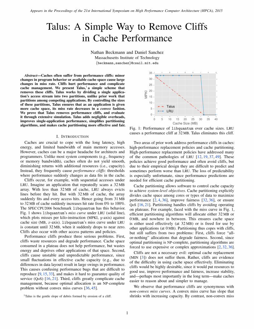
Fig. 1 shows libquantum’s miss curve under LRU (solid line),

which plots misses per kilo-instruction (MPKI, y-axis) against

cache size (MB, x-axis). libquantum’s miss curve under LRU

is constant until 32 MB, when it suddenly drops to near zero.

Cliffs also occur with other access patterns and policies.Performance cliffs produce three serious problems. First,

cliffs waste resources and degrade performance. Cache space

consumed in a plateau does not help performance, but wastes

energy and deprives other applications of that space. Second,

cliffs cause unstable and unpredictable performance, since

small fluctuations in effective cache capacity (e.g., due to

differences in data layout) result in large swings in performance.

This causes confusing performance bugs that are difficult to

reproduce [9, 15, 33], and makes it hard to guarantee quality of

service (QoS) [16, 21]. Third, cliffs greatly complicate cache

management, because optimal allocation is an NP-complete

problem without convex miss curves [36, 45].

1Talus is the gentle slope of debris formed by erosion of a cliff.

0 5 10 15 20 25 30 35 40

Cache Size (MB)

0

5

10

15

20

25

30

35

MP

KI

Talus

LRU

Fig. 1: Performance of libquantum over cache sizes. LRU

causes a performance cliff at 32 MB. Talus eliminates this cliff.

Two areas of prior work address performance cliffs in caches:

high-performance replacement policies and cache partitioning.

High-performance replacement policies have addressed many

of the common pathologies of LRU [12, 19, 37, 49]. These

policies achieve good performance and often avoid cliffs, but

due to their empirical design they are difficult to predict and

sometimes perform worse than LRU. The loss of predictability

is especially unfortunate, since performance predictions are

needed for efficient cache partitioning.

Cache partitioning allows software to control cache capacity

to achieve system-level objectives. Cache partitioning explicitly

divides cache space among cores or types of data to maximize

performance [2, 4, 36], improve fairness [32, 36], or ensure

QoS [16, 21]. Partitioning handles cliffs by avoiding operating

on plateaus. For example, faced with the miss curve in Fig. 1,

efficient partitioning algorithms will allocate either 32 MB or

0 MB, and nowhere in between. This ensures cache space

is either used effectively (at 32 MB) or is freed for use by

other applications (at 0 MB). Partitioning thus copes with cliffs,

but still suffers from two problems: First, cliffs force “all-

or-nothing” allocations that degrade fairness. Second, since

optimal partitioning is NP-complete, partitioning algorithms are

forced to use expensive or complex approximations [2, 32, 36].

Cliffs are not a necessary evil: optimal cache replacement

(MIN [3]) does not suffer them. Rather, cliffs are evidence

of the difficulty in using cache space effectively. Eliminating

cliffs would be highly desirable, since it would put resources to

good use, improve performance and fairness, increase stability,

and—perhaps most importantly in the long term—make caches

easier to reason about and simpler to manage.

We observe that performance cliffs are synonymous with

non-convex miss curves. A convex miss curve has slope that

shrinks with increasing capacity. By contrast, non-convex miss

1

curves have regions of small slope (plateaus) followed by

regions of larger slope (cliffs). Convexity means that additional

capacity gives smooth and diminishing hit rate improvements.

We present Talus, a simple partitioning technique that ensures

convex miss curves and thus eliminates performance cliffs in

caches. Talus achieves convexity by partitioning within a single

access stream, as opposed to prior work that partitions among

competing access streams. Talus divides accesses between two

shadow partitions, invisible to software, that emulate caches of

a larger and smaller size. By choosing these sizes judiciously,

Talus ensures convexity and improves performance. Our key

insight is that only the miss curve is needed to do this. We

make the following contributions:

• We present Talus, a simple method to remove performance

cliffs in caches. Talus operates on miss curves, and works

with any replacement policy whose miss curve is available.

• We prove Talus’s convexity and generality under broad

assumptions that are satisfied in practice.

• We design Talus to be predictable: its miss curve is trivially

derived from the underlying policy’s miss curve, making

Talus easy to use in cache partitioning.

• We contrast Talus with bypassing, a common replacement

technique. We derive the optimal bypassing scheme and show

that Talus is superior, and discuss the implications of this

result on the design of replacement policies.

• We develop a practical, low-overhead implementation of

Talus that works with existing partitioning schemes and

requires negligible hardware and software overheads.

• We evaluate Talus under simulation. Talus transforms LRU

into a policy free of cliffs and competitive with state-of-

the-art replacement policies [12, 19, 37]. More importantly,

Talus’s convexity simplifies cache partitioning algorithms,

and automatically improves their performance and fairness.

In short, Talus is the first approach to offer both the benefits

of high-performance cache replacement and the versatility of

software control through cache partitioning.

II. BACKGROUND AND INSIGHTS

We first review relevant work in cache replacement and

partitioning, and develop the insights behind Talus.

A. Replacement policies

The optimal replacement policy, Belady’s MIN [3, 30], relies

on a perfect oracle to replace the line that will be reused furthest

in the future. Prior work has proposed many mechanisms and

heuristics that attempt to emulate optimal replacement. We

observe that, details aside, they use three broad techniques:

• Recency: Recency prioritizes recently used lines over old

ones. LRU uses recency alone, which has obvious pathologies

(e.g., thrashing and scanning [10, 37]). Most high-perfor-

mance policies combine recency with other techniques.

• Classification: Some policies divide lines into separate

classes, and treat lines of each class differently. For example,

several policies classify lines as reused or non-reused [19, 24].

Classification works well when classes have markedly

different access patterns.

• Protection: When the working set does not fit in the cache,

some policies choose to protect a portion of the working

set against eviction from other lines to avoid thrashing.

Protection is equivalent to thrash-resistance [19, 37].High-performance policies implement these techniques in

different ways. DIP [37] enhances LRU by dynamically detect-

ing thrashing using set dueling, and protects lines in the cache

by inserting most lines at low priority in the LRU chain. DIP

inserts a fixed fraction of lines (ǫ = 1/32) at high priority

to avoid stale lines. DRRIP [19] classifies between reused

and non-reused lines by inserting lines at medium priority,

includes recency by promoting lines on reuse, and protects

against thrashing with the same mechanism as DIP. SHiP [49]

extends DRRIP with more elaborate classification, based on

the memory address, PC, or instruction sequence. PDP [12]

decides how long to protect lines based on the reuse distance

distribution, but does not do classification. IbRDP [22] uses

PC-based classification, but does not do protection.These policies improve over LRU on average, but have two

main drawbacks. First, these policies use empirically tuned

heuristics that may not match application behavior, so they

sometimes perform worse than LRU (Sec. VII-C). Second, and

more importantly, the miss curve for these policies cannot be

easily estimated in general, which makes them hard to use

with partitioning, as we discuss next.

B. Cache partitioning

Cache partitioning allows software to divide space among

cores, threads, or types of data [2, 7, 40], enabling system-

wide management of shared caches. There are several ways

to implement partitioning schemes. Way partitioning [1, 7] is

simple and commonly used, but it allows only few coarse

partitions and degrades associativity. Fine-grained partitioning

techniques like Vantage [40] and Futility Scaling [48] support

hundreds of inexpensive partitions sized in cache lines, and

strictly enforce these sizes. Finally, set partitioning can be

implemented in hardware through reconfigurable or molecular

caches [38, 47], or in software by using page coloring [29].Replacement policies vs. partitioning: Cache partitioning

is often used to improve performance in systems with shared

caches [32, 36, 44], and is sometimes compared to thread-aware

extensions of several replacement policies [12, 17, 19]. However,

cache partitioning has many other uses beyond performance,

and is better thought of as an enabling technology for software

control of the cache. Partitioning strikes a nice balance between

scratchpad memories, which yield control to software but are

hard to use, and conventional hardware-only caches, which are

easy to use but opaque to software. For instance, partitioning

has been used to improve fairness [32, 35], implement priorities

and guarantee QoS [8, 13, 21], improve NUCA designs [2, 28],

and eliminate side-channel attacks [34]. Talus adds another

capability to partitioning: eliminating cache performance cliffs.Partitioning is therefore a general tool to help achieve system-

level objectives. After all, caches consume over half of chip

area in modern processors [27]; surely, software should have a

say in how they are used. Hardware-only replacement policies

simply do not support this—they use policies fixed at design

time and cannot know what to optimize for.

C. Predictability

We say that a replacement policy is predictable if the miss

curve, i.e. its miss rate on a given access stream at different

2

partition sizes, can be estimated efficiently. Miss curves allow

partitioning policies to reason about the effect of different

partition sizes without actually running and measuring perfor-

mance at each size. Using miss curves, dynamic partitioning

algorithms can find and set the appropriate sizes without trial

and error. Because resizing partitions is slow and the space of

choices is very large, predictability is highly desirable.

The need for predictability has confined partitioning to

LRU in practice. LRU’s miss curve can be cheaply sampled

in hardware using utility monitors (UMONs) [36], or in

software using address-based sampling [11, 42]. However, high-

performance replacement policies lack this predictability. Since

they are designed empirically and do not obey the stack

property [30], there is no simple known monitoring scheme

that can sample their miss curve cheaply. Likewise, much work

has gone into modeling LRU’s performance for general access

patterns, but little for high-performance policies. For example,

DIP was analyzed on cyclic, scanning access patterns [37] (e.g.,

libquantum in Fig. 1). While insightful, this analysis does

not extend to general access patterns that do not exhibit cyclic

behavior (e.g., Fig. 3 in Sec. III; see also Sec. V-C).

Alternatively, non-predictable policies can adapt through

slow trial and error [8, 14]. However, these schemes can get

stuck in local optima, scale poorly beyond few cores, and are

unresponsive to changes in application behavior since partitions

take tens of milliseconds to be resized.

Convexity is thus not a substitute for predictability. Some

high-performance policies are mostly convex in practice (e.g.,

DRRIP [19], Fig. 10), but without some way of predicting their

performance, such policies cannot be effectively controlled by

software to achieve system-level objectives.

High-performance cache replacement and partitioning are

consequently at loggerheads: techniques that improve single-

thread performance are incompatible with those used to manage

shared caches. This is unfortunate, since in principle they

should be complementary. A key contribution of Talus is to

eliminate this conflict by capturing much of the benefit of high-

performance policies without sacrificing LRU’s predictability.

D. Convexity

Convexity means that the miss curve’s slope shrinks as cache

space grows [45]. Convexity implies that the cache yields

diminishing returns on performance with increasing cache

space, and thus implies the absence of cliffs. It has two other

important benefits: it makes simple allocation algorithms (e.g.,

hill climbing) optimal, and it avoids all-or-nothing behavior,

improving fairness. Although the benefits of convexity may not

be obvious, prior work shows that there is latent demand for

convex cache behavior in order to simplify cache management.

Simple resource allocation: Without convexity, partitioning

cache capacity to maximize performance is an NP-complete

problem [45]. Existing algorithms yield approximate and

often good solutions, but they are either inefficient [36] or

complex [2, 32]. This makes them hard to apply to large-scale

systems or multi-resource management [4]. Alternatively, prior

work consciously ignores non-convexity and applies convex

optimization [4, 8], sacrificing performance for simplicity and

reduced overheads. As we will see in Sec. VII, applying

convex optimization to LRU wipes out most of the benefits of

partitioning. Thus, it is not surprising that prior techniques that

use hill climbing or local optimization methods to partition LRU

find little benefit [4, 8], and those that use more sophisticated

methods, such as Lookahead or dynamic programming, report

significant gains [2, 21, 32, 36, 40, 50].

Convexity eliminates this tradeoff, as cheap convex opti-

mization (e.g., hill climbing) finds the optimal sizes [5, 45].

By ensuring convexity, Talus simplifies cache management.

Fairness: Even if optimization complexity is not a concern,

eliminating cliffs also avoids all-or-nothing behavior in alloca-

tions and improves fairness. For example, imagine a system

with a 32 MB cache running two instances of libquantum

(with miss curve shown in Fig. 1, solid line). If the cache is

unpartitioned, both applications will evict each other’s lines,

getting no hits (both will have effective capacity below the

32 MB cliff). Partitioning can help one of the applications by

giving it the whole 32 MB cache, but this is unfair. Any other

choice of partition sizes will yield no benefit. Imbalanced par-

titioning [35] finds that this is common in parallel applications,

and proposes to allocate most cache space to a single thread

of a homogeneous parallel application to improve performance.

Convex miss curves make this unnecessary: with Talus’ miss

curve (Fig. 1, dashed line), giving 16 MB to each instance of

libquantum accelerates both instances equally and maximizes

the cache’s hit rate. In general, with homogeneous threads

and convex miss curves, the maximum-utility point is equal

allocations, which is also the most fair.

In summary, convexity not only provides smooth, stable be-

havior, but makes optimal resource allocation cheap, improves

fairness, and leads to better allocation outcomes.

III. TALUS EXAMPLE

This section illustrates how Talus works with a simple

example. Talus uses partitioning to eliminate cache performance

cliffs. Unlike prior work that partitions capacity among different

cores, Talus partitions within a single access stream. It does so

by splitting the cache (or, in partitioned caches, each software-

visible partition) into two hidden shadow partitions. It then

controls the size of these partitions and how accesses are

distributed between them to achieve the desired performance.

Talus computes the appropriate shadow partition configura-

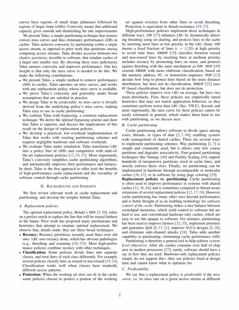
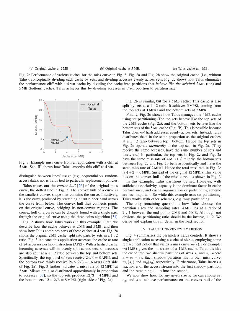
tion using miss curves; in this example we use the miss curve

in Fig. 3. Fig. 3 is the miss curve of LRU on an application

that accesses 2 MB of data at random, and an additional 3 MB

sequentially. This results in a performance cliff around 5 MB,

when MPKI suddenly drops from 12 to 3 once the application’s

data fits in the cache. Since the cache gets 12 MPKI at 2 MB,

there is no benefit from additional capacity from 2 until 5 MB.

Hence at 4 MB, half of the cache is essentially wasted since it

could be left unused with no loss in performance.

Talus can eliminate this cliff and improve performance.

Specifically, in this example Talus achieves 6 MPKI at 4 MB.

The key insight is that LRU is inefficient at 4 MB, but LRU is

efficient at 2 MB and 5 MB. Talus thus makes part of the cache

behave like a 2 MB cache, and the rest behave like a 5 MB

cache. As a result, the 4 MB cache behaves like a combination

of efficient caches, and is itself efficient. Significantly, Talus

requires only the miss curve to ensure convexity. Talus is

totally blind to the behavior of individual lines, and does not

3

1224

4/3 MB

2/3 MB

Accesses

(APKI)Misses

(MPKI)

(a) Original cache at 2 MB.

324

Accesses

(APKI)Misses

(MPKI)5/3 MB

10/3 MB

(b) Original cache at 5 MB.

624

Accesses

(APKI)Misses

(MPKI)2/3 MB

10/3 MB

(c) Talus cache at 4 MB.

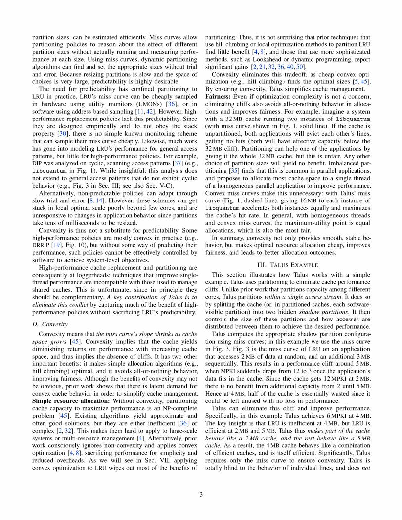
Fig. 2: Performance of various caches for the miss curve in Fig. 3. Fig. 2a and Fig. 2b show the original cache (i.e., without

Talus), conceptually dividing each cache by sets, and dividing accesses evenly across sets. Fig. 2c shows how Talus eliminates

the performance cliff with a 4 MB cache by dividing the cache into partitions that behave like the original 2 MB (top) and

5 MB (bottom) caches. Talus achieves this by dividing accesses in dis-proportion to partition size.

0 2 4 6 8 10

Cache size (MB)

0

5

10

15

20

25

Mis

ses (

MP

KI)

Example(Fig. 2c)

Original

Talus

Fig. 3: Example miss curve from an application with a cliff at

5 MB. Sec. III shows how Talus smooths this cliff at 4 MB.

distinguish between lines’ usage (e.g., sequential vs. random-

access data), nor is Talus tied to particular replacement policies.

Talus traces out the convex hull [26] of the original miss

curve, the dotted line in Fig. 3. The convex hull of a curve is

the smallest convex shape that contains the curve. Intuitively,

it is the curve produced by stretching a taut rubber band across

the curve from below. The convex hull thus connects points

on the original curve, bridging its non-convex regions. The

convex hull of a curve can be cheaply found with a single pass

through the original curve using the three-coins algorithm [31].

Fig. 2 shows how Talus works in this example. First, we

describe how the cache behaves at 2 MB and 5 MB, and then

show how Talus combines parts of these caches at 4 MB. Fig. 2a

shows the original 2 MB cache, split into parts by sets in a 1 : 2

ratio. Fig. 3 indicates this application accesses the cache at rate

of 24 accesses per kilo-instruction (APKI). With a hashed cache,

incoming accesses will be evenly split across sets, so accesses

are also split at a 1 : 2 ratio between the top and bottom sets.

Specifically, the top third of sets receive 24/3 = 8APKI, and

the bottom two thirds receive 24× 2/3 = 16APKI (left side

of Fig. 2a). Fig. 3 further indicates a miss rate of 12 MPKI at

2 MB. Misses are also distributed approximately in proportion

to accesses [37], so the top sets produce 12/3 = 4MPKI and

the bottom sets 12× 2/3 = 8MPKI (right side of Fig. 2a).

Fig. 2b is similar, but for a 5 MB cache. This cache is also

split by sets at a 1 : 2 ratio. It achieves 3 MPKI, coming from

the top sets at 1 MPKI and the bottom sets at 2 MPKI.

Finally, Fig. 2c shows how Talus manages the 4 MB cache

using set partitioning. The top sets behave like the top sets of

the 2 MB cache (Fig. 2a), and the bottom sets behave like the

bottom sets of the 5 MB cache (Fig. 2b). This is possible because

Talus does not hash addresses evenly across sets. Instead, Talus

distributes them in the same proportion as the original caches,

at a 1 : 2 ratio between top : bottom. Hence the top sets in

Fig. 2c operate identically to the top sets in Fig. 2a. (They

receive the same accesses, have the same number of sets and

lines, etc.) In particular, the top sets in Fig. 2c and Fig. 2a

have the same miss rate of 4 MPKI. Similarly, the bottom sets

between Fig. 2c and Fig. 2b behave identically and have the

same miss rate of 2 MPKI. Hence the total miss rate in Fig. 2c

is 4+2 = 6MPKI (instead of the original 12 MPKI). This value

lies on the convex hull of the miss curve, as shown in Fig. 3.

In this example, Talus partitions by set. However, with

sufficient associativity, capacity is the dominant factor in cache

performance, and cache organization or partitioning scheme

are less important. So while this example uses set partitioning,

Talus works with other schemes, e.g. way partitioning.

The only remaining question is how Talus chooses the

partition sizes and sampling rates. 4 MB lies at a ratio of

2 : 1 between the end points 2 MB and 5 MB. Although not

obvious, the partitioning ratio should be the inverse, 1 : 2. We

derive and explain this in detail in the next section.

IV. TALUS: CONVEXITY BY DESIGN

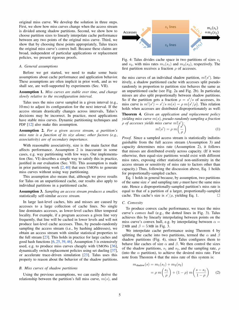
Fig. 4 summarizes the parameters Talus controls. It shows a

single application accessing a cache of size s, employing some

replacement policy that yields a miss curve m(s). For example,

m(1 MB) gives the miss rate of a 1 MB cache. Talus divides

the cache into two shadow partitions of sizes s1 and s2, where

s = s1 + s2. Each shadow partition has its own miss curve,

m1(s1) and m2(s2) respectively. Furthermore, Talus inserts a

fraction ρ of the access stream into the first shadow partition,

and the remaining 1− ρ into the second.

We now show how, for any given size s, we can choose s1,

s2, and ρ to achieve performance on the convex hull of the

4

original miss curve. We develop the solution in three steps.

First, we show how miss curves change when the access stream

is divided among shadow partitions. Second, we show how to

choose partition sizes to linearly interpolate cache performance

between any two points of the original miss curve. Third, we

show that by choosing these points appropriately, Talus traces

the original miss curve’s convex hull. Because these claims are

broad, independent of particular applications or replacement

policies, we present rigorous proofs.

A. General assumptions

Before we get started, we need to make some basic

assumptions about cache performance and application behavior.

These assumptions are often implicit in prior work, and as we

shall see, are well-supported by experiments (Sec. VII).

Assumption 1. Miss curves are stable over time, and change

slowly relative to the reconfiguration interval.

Talus uses the miss curve sampled in a given interval (e.g.,

10 ms) to adjust its configuration for the next interval. If the

access stream drastically changes across intervals, Talus’s

decisions may be incorrect. In practice, most applications

have stable miss curves. Dynamic partitioning techniques and

PDP [12] also make this assumption.

Assumption 2. For a given access stream, a partition’s

miss rate is a function of its size alone; other factors (e.g.,

associativity) are of secondary importance.

With reasonable associativity, size is the main factor that

affects performance. Assumption 2 is inaccurate in some

cases, e.g. way partitioning with few ways. Our implementa-

tion (Sec. VI) describes a simple way to satisfy this in practice,

justified in our evaluation (Sec. VII). This assumption is made

in prior partitioning work [2, 40] that uses UMONs to generate

miss curves without using way partitioning.

This assumption also means that, although we prove results

for Talus on an unpartitioned cache, our results also apply to

individual partitions in a partitioned cache.

Assumption 3. Sampling an access stream produces a smaller,

statistically self-similar access stream.

In large last-level caches, hits and misses are caused by

accesses to a large collection of cache lines. No single

line dominates accesses, as lower-level caches filter temporal

locality. For example, if a program accesses a given line very

frequently, that line will be cached in lower levels and will not

produce last-level cache accesses. Thus, by pseudo-randomly

sampling the access stream (i.e., by hashing addresses), we

obtain an access stream with similar statistical properties to

the full stream [23]. This holds in practice for large caches and

good hash functions [6, 25, 39, 46]. Assumption 3 is extensively

used, e.g. to produce miss curves cheaply with UMONs [36],

dynamically switch replacement policies using set dueling [37],

or accelerate trace-driven simulation [23]. Talus uses this

property to reason about the behavior of the shadow partitions.

B. Miss curves of shadow partitions

Using the previous assumptions, we can easily derive the

relationship between the partition’s full miss curve, m(s), and

� lines

� �+� �Accesses

� lines

Fig. 4: Talus divides cache space in two partitions of sizes s1and s2, with miss rates m1(s1) and m2(s2), respectively. The

first partition receives a fraction ρ of accesses.

the miss curves of an individual shadow partition, m′(s′). Intu-

itively, a shadow partitioned cache with accesses split pseudo-

randomly in proportion to partition size behaves the same as

an unpartitioned cache (see Fig. 2a and Fig. 2b). In particular,

misses are also split proportionally between shadow partitions.

So if the partition gets a fraction ρ = s′/s of accesses, its

miss curve is m′(s′) = s′/s m(s) = ρ m(

s′/ρ)

. This relation

holds when accesses are distributed disproportionately as well:

Theorem 4. Given an application and replacement policy

yielding miss curve m(s), pseudo-randomly sampling a fraction

ρ of accesses yields miss curve m′(s′):

m′(s′) = ρ m

(

s′

ρ

)

(1)

Proof. Since a sampled access stream is statistically indistin-

guishable from the full access stream (Assumption 3) and

capacity determines miss rate (Assumption 2), it follows

that misses are distributed evenly across capacity. (If it were

otherwise, then equal-size partitions would exist with different

miss rates, exposing either statistical non-uniformity in the

access stream or sensitivity of miss rate to factors other than

capacity.) Thus, following the discussion above, Eq. 1 holds

for proportionally-sampled caches.

Eq. 1 holds in general because, by assumption, two partitions

of the same size s′ and sampling rate ρ must have the same miss

rate. Hence a disproportionally-sampled partition’s miss rate is

equal to that of a partition of a larger, proportionally-sampled

cache. This cache’s size is s′/ρ, yielding Eq. 1.

C. Convexity

To produce convex cache performance, we trace the miss

curve’s convex hull (e.g., the dotted lines in Fig. 3). Talus

achieves this by linearly interpolating between points on the

miss curve’s convex hull, e.g. by interpolating between α =2MB and β = 5MB in Fig. 3.

We interpolate cache performance using Theorem 4 by

splitting the cache into two partitions, termed the α and βshadow partitions (Fig. 4), since Talus configures them to

behave like caches of size α and β. We then control the sizes

of the shadow partitions, s1 and s2, and the sampling rate, ρ(into the α partition), to achieve the desired miss rate. First

note from Theorem 4 that the miss rate of this system is:

mshadow(s) = m1(s1) +m2(s2)

= ρ m

(

s1ρ

)

+ (1− ρ) m

(

s− s11− ρ

)

(2)

5

Lemma 5. Given an application and replacement policy

yielding miss curve m(·), one can achieve miss rate at size

s that linearly interpolates between any two points on on the

curve, m(α) and m(β), where α ≤ s < β.

Proof. To interpolate, we must anchor terms in mshadow at

m(α) and m(β). We wish to do so for all m, in particular

injective m, hence anchoring the first term at m(α) implies:

m(s1/ρ) = m(α) ⇒ s1 = ρα (3)

Anchoring the second term at m(β) implies:

m

(

s− s11− ρ

)

= m(β) ⇒ ρ =β − s

β − α(4)

Substituting these values into the above equation yields:

mshadow =β − s

β − αm(α) +

s− α

β − αm(β) (5)

Hence as s varies from α to β, the system’s miss rate varies

proportionally between m(α) to m(β) as desired.

Theorem 6. Given a replacement policy and application

yielding miss curve m(s), Talus produces a new replacement

policy that traces the miss curve’s convex hull.

Proof. Set sizes α and β to be the neighboring points around

s along m’s convex hull and apply Lemma 5. That is, α is the

largest cache size no greater than s where the original miss

curve m and its convex hull coincide, and β is the smallest

cache size larger than s where they coincide.

Finally, we now apply Theorem 6 to Fig. 2 to show how the

partition sizes and sampling rate were derived for a s = 4MB

cache. We begin by choosing α = 2MB and β = 5MB, as

these are the neighboring points on the convex hull (Fig. 3). ρis the “normalized distance to β”: 4 MB is two-thirds of the

way to 5 MB from 2 MB, so one third remains and ρ = 1/3. s1is the partition size that will emulate a cache size of α with

this sampling rate. By Theorem 4, s1 = ρ α = 2/3 MB. Finally,

s2 is the remaining cache space, 10/3 MB. This size works

because—by design—it emulates a cache of size β: the second

partition’s sampling rate is 1 − ρ = 2/3, so by Theorem 4 it

models a cache of size s2/(1− ρ) = 5MB.

Hence, a fraction ρ = 1/3 of accesses behave like a α = 2MB

cache, and the rest behave like a β = 5MB cache. This fraction

changes as s moves between α and β, smoothly interpolating

performance between points on the convex hull.

V. THEORETICAL IMPLICATIONS

A few interesting results follow from the previous section.

All of the following should be taken to hold approximately in

practice, since the assumptions only hold approximately.

A. Predictability enables convexity

Theorem 6 says that so long as the miss curve is available,

it is fairly simple to ensure convex performance by applying

Talus. While Talus is general (we later show how it convexifies

SRRIP, albeit using impractically large monitors), it is currently

most practical with policies in the LRU family [42]. Talus

motivates further development of high-performance policies

for which the miss curve can be cheaply obtained.

0 2 4 6 8 10

Cache size (MB)

0

5

10

15

20

25

Mis

ses (

MP

KI)

Optimalbypassingat 4MB Original

Non-bypassed

+ Bypassed

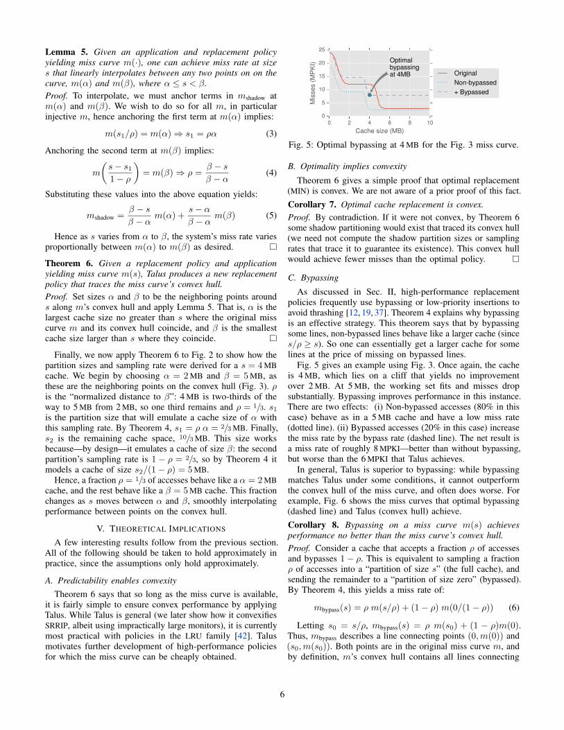
Fig. 5: Optimal bypassing at 4 MB for the Fig. 3 miss curve.

B. Optimality implies convexity

Theorem 6 gives a simple proof that optimal replacement

(MIN) is convex. We are not aware of a prior proof of this fact.

Corollary 7. Optimal cache replacement is convex.

Proof. By contradiction. If it were not convex, by Theorem 6

some shadow partitioning would exist that traced its convex hull

(we need not compute the shadow partition sizes or sampling

rates that trace it to guarantee its existence). This convex hull

would achieve fewer misses than the optimal policy.

C. Bypassing

As discussed in Sec. II, high-performance replacement

policies frequently use bypassing or low-priority insertions to

avoid thrashing [12, 19, 37]. Theorem 4 explains why bypassing

is an effective strategy. This theorem says that by bypassing

some lines, non-bypassed lines behave like a larger cache (since

s/ρ ≥ s). So one can essentially get a larger cache for some

lines at the price of missing on bypassed lines.

Fig. 5 gives an example using Fig. 3. Once again, the cache

is 4 MB, which lies on a cliff that yields no improvement

over 2 MB. At 5 MB, the working set fits and misses drop

substantially. Bypassing improves performance in this instance.

There are two effects: (i) Non-bypassed accesses (80% in this

case) behave as in a 5 MB cache and have a low miss rate

(dotted line). (ii) Bypassed accesses (20% in this case) increase

the miss rate by the bypass rate (dashed line). The net result is

a miss rate of roughly 8 MPKI—better than without bypassing,

but worse than the 6 MPKI that Talus achieves.

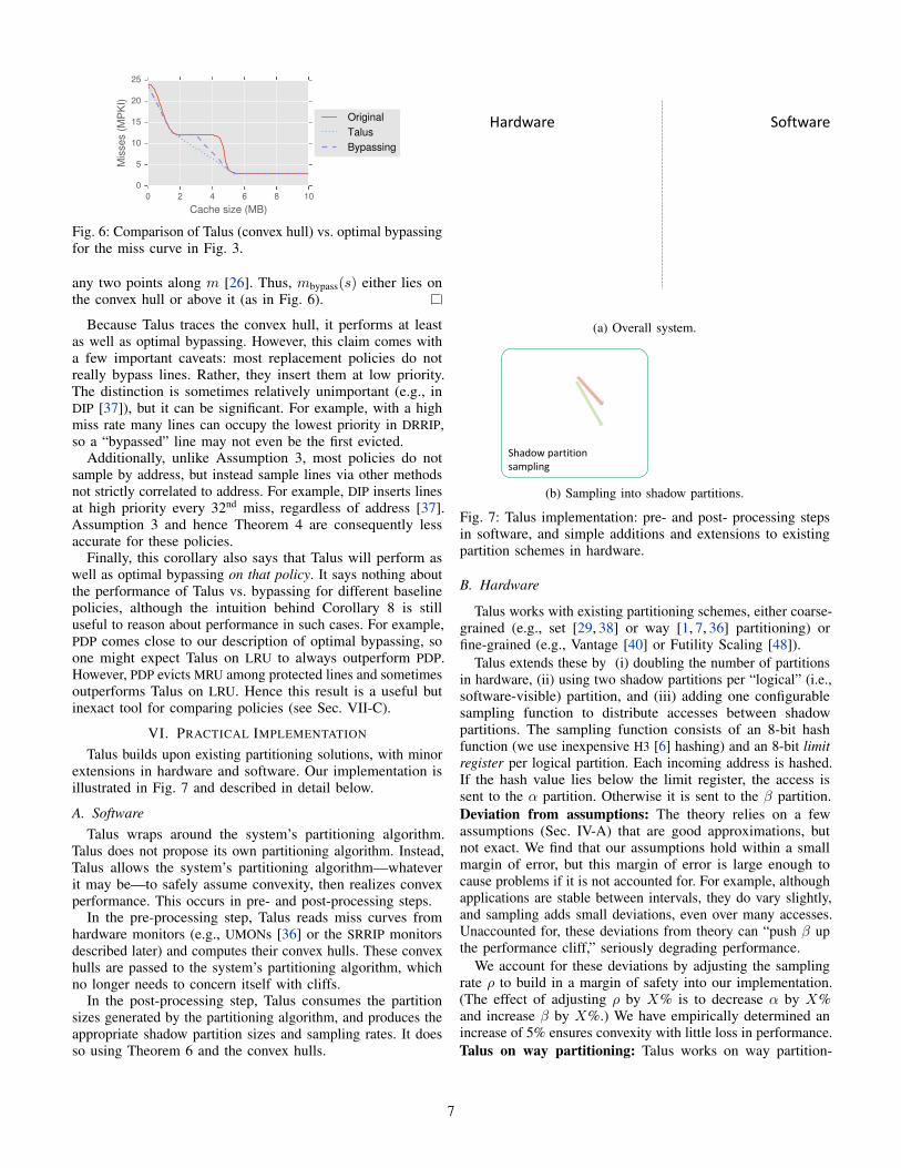
In general, Talus is superior to bypassing: while bypassing

matches Talus under some conditions, it cannot outperform

the convex hull of the miss curve, and often does worse. For

example, Fig. 6 shows the miss curves that optimal bypassing

(dashed line) and Talus (convex hull) achieve.

Corollary 8. Bypassing on a miss curve m(s) achieves

performance no better than the miss curve’s convex hull.

Proof. Consider a cache that accepts a fraction ρ of accesses

and bypasses 1− ρ. This is equivalent to sampling a fraction

ρ of accesses into a “partition of size s” (the full cache), and

sending the remainder to a “partition of size zero” (bypassed).

By Theorem 4, this yields a miss rate of:

mbypass(s) = ρ m(s/ρ) + (1− ρ) m(0/(1− ρ)) (6)

Letting s0 = s/ρ, mbypass(s) = ρ m(s0) + (1 − ρ)m(0).Thus, mbypass describes a line connecting points (0,m(0)) and

(s0,m(s0)). Both points are in the original miss curve m, and

by definition, m’s convex hull contains all lines connecting

6

0 2 4 6 8 10

Cache size (MB)

0

5

10

15

20

25

Mis

ses (

MP

KI)

Original

Talus

Bypassing

Fig. 6: Comparison of Talus (convex hull) vs. optimal bypassing

for the miss curve in Fig. 3.

any two points along m [26]. Thus, mbypass(s) either lies on

the convex hull or above it (as in Fig. 6).

Because Talus traces the convex hull, it performs at least

as well as optimal bypassing. However, this claim comes with

a few important caveats: most replacement policies do not

really bypass lines. Rather, they insert them at low priority.

The distinction is sometimes relatively unimportant (e.g., in

DIP [37]), but it can be significant. For example, with a high

miss rate many lines can occupy the lowest priority in DRRIP,

so a “bypassed” line may not even be the first evicted.Additionally, unlike Assumption 3, most policies do not

sample by address, but instead sample lines via other methods

not strictly correlated to address. For example, DIP inserts lines

at high priority every 32nd miss, regardless of address [37].

Assumption 3 and hence Theorem 4 are consequently less

accurate for these policies.Finally, this corollary also says that Talus will perform as

well as optimal bypassing on that policy. It says nothing about

the performance of Talus vs. bypassing for different baseline

policies, although the intuition behind Corollary 8 is still

useful to reason about performance in such cases. For example,

PDP comes close to our description of optimal bypassing, so

one might expect Talus on LRU to always outperform PDP.

However, PDP evicts MRU among protected lines and sometimes

outperforms Talus on LRU. Hence this result is a useful but

inexact tool for comparing policies (see Sec. VII-C).

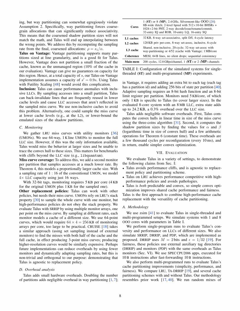
VI. PRACTICAL IMPLEMENTATION

Talus builds upon existing partitioning solutions, with minor

extensions in hardware and software. Our implementation is

illustrated in Fig. 7 and described in detail below.

A. Software

Talus wraps around the system’s partitioning algorithm.

Talus does not propose its own partitioning algorithm. Instead,

Talus allows the system’s partitioning algorithm—whatever

it may be—to safely assume convexity, then realizes convex

performance. This occurs in pre- and post-processing steps.In the pre-processing step, Talus reads miss curves from

hardware monitors (e.g., UMONs [36] or the SRRIP monitors

described later) and computes their convex hulls. These convex

hulls are passed to the system’s partitioning algorithm, which

no longer needs to concern itself with cliffs.In the post-processing step, Talus consumes the partition

sizes generated by the partitioning algorithm, and produces the

appropriate shadow partition sizes and sampling rates. It does

so using Theorem 6 and the convex hulls.

Talus modifies UnmodifiedTalus additions

SoftwareHardwareMiss curve

monitors

Pre-

processing

Partitioning

Algorithm

Post-

processing

Desired

allocations

Convex hulls

Shadow partition sizes

& sampling rate

Miss curves

Co

nve

x h

ull

s

Partitioned Cache

Log

ica

l p

art

itio

n

(a) Overall system.

Shadow partition

sampling

H3

hash

Limit

RegAddress

Limit

Reg

…

Partitioned Cache

(b) Sampling into shadow partitions.

Fig. 7: Talus implementation: pre- and post- processing steps

in software, and simple additions and extensions to existing

partition schemes in hardware.

B. Hardware

Talus works with existing partitioning schemes, either coarse-

grained (e.g., set [29, 38] or way [1, 7, 36] partitioning) or

fine-grained (e.g., Vantage [40] or Futility Scaling [48]).

Talus extends these by (i) doubling the number of partitions

in hardware, (ii) using two shadow partitions per “logical” (i.e.,

software-visible) partition, and (iii) adding one configurable

sampling function to distribute accesses between shadow

partitions. The sampling function consists of an 8-bit hash

function (we use inexpensive H3 [6] hashing) and an 8-bit limit

register per logical partition. Each incoming address is hashed.

If the hash value lies below the limit register, the access is

sent to the α partition. Otherwise it is sent to the β partition.

Deviation from assumptions: The theory relies on a few

assumptions (Sec. IV-A) that are good approximations, but

not exact. We find that our assumptions hold within a small

margin of error, but this margin of error is large enough to

cause problems if it is not accounted for. For example, although

applications are stable between intervals, they do vary slightly,

and sampling adds small deviations, even over many accesses.

Unaccounted for, these deviations from theory can “push β up

the performance cliff,” seriously degrading performance.

We account for these deviations by adjusting the sampling

rate ρ to build in a margin of safety into our implementation.

(The effect of adjusting ρ by X% is to decrease α by X%

and increase β by X%.) We have empirically determined an

increase of 5% ensures convexity with little loss in performance.

Talus on way partitioning: Talus works on way partition-

7

ing, but way partitioning can somewhat egregiously violate

Assumption 2. Specifically, way partitioning forces coarse-

grain allocations that can significantly reduce associativity.

This means that the coarsened shadow partition sizes will not

match the math, and Talus will end up interpolating between

the wrong points. We address this by recomputing the sampling

rate from the final, coarsened allocations: ρ = s1/α.

Talus on Vantage: Vantage partitioning supports many par-

titions sized at line granularity, and is a good fit for Talus.

However, Vantage does not partition a small fraction of the

cache, known as the unmanaged region (10% of the cache in

our evaluation). Vantage can give no guarantees on capacity for

this region. Hence, at a total capacity of s, our Talus-on-Vantage

implementation assumes a capacity of s′ = 0.9s. Using Talus

with Futility Scaling [48] would avoid this complication.

Inclusion: Talus can cause performance anomalies with inclu-

sive LLCs. By sampling accesses into a small partition, Talus

can back-invalidate lines that are frequently reused in lower

cache levels and cause LLC accesses that aren’t reflected in

the sampled miss curve. We use non-inclusive caches to avoid

this problem. Alternatively, one could sample the miss curve

at lower cache levels (e.g., at the L2), or lower-bound the

emulated sizes of the shadow partitions.

C. Monitoring

We gather LRU miss curves with utility monitors [36]

(UMONs). We use 64-way, 1 K line UMONs to monitor the full

LLC size. However, if this was the only information available,

Talus would miss the behavior at larger sizes and be unable to

trace the convex hull to these sizes. This matters for benchmarks

with cliffs beyond the LLC size (e.g., libquantum).

Miss curve coverage: To address this, we add a second monitor

per partition that samples accesses at a much lower rate. By

Theorem 4, this models a proportionally larger cache size. With

a sampling rate of 1 : 16 of the conventional UMON, we model

4× LLC capacity using just 16 ways.

With 32-bit tags, monitoring requires 5 KB per core (4 KB

for the original UMON plus 1 KB for the sampled one).

Other replacement policies: Talus can work with other

policies, but needs their miss curve. UMONs rely on LRU’s stack

property [30] to sample the whole curve with one monitor, but

high-performance policies do not obey the stack property. We

evaluate Talus with SRRIP by using multiple monitor arrays, one

per point on the miss curve. By sampling at different rates, each

monitor models a cache of a different size. We use 64-point

curves, which would require 64× 4 = 256KB of monitoring

arrays per core, too large to be practical. CRUISE [18] takes

a similar approach (using set sampling instead of external

monitors) to find the misses with both half of the cache and the

full cache, in effect producing 3-point miss curves; producing

higher-resolution curves would be similarly expensive. Perhaps

future implementations can reduce overheads by using fewer

monitors and dynamically adapting sampling rates, but this is

non-trivial and orthogonal to our purpose: demonstrating that

Talus is agnostic to replacement policy.

D. Overhead analysis

Talus adds small hardware overheads. Doubling the number

of partitions adds negligible overhead in way partitioning [1, 7];

Cores

1 (ST) or 8 (MP), 2.4 GHz, Silvermont-like OOO [20]:8B-wide ifetch; 2-level bpred with 512×10-bit BHSRs +1024×2-bit PHT, 2-way decode/issue/rename/commit,32-entry IQ and ROB, 10-entry LQ, 16-entry SQ

L1 caches 32 KB, 8-way set-associative, split D/I, 4-cycle latency

L2 caches 128 KB priv per-core, 8-way set-assoc, inclusive, 6-cycle

L3 cacheShared, non-inclusive, 20-cycle; 32-way set-assoc withway-partitioning or 4/52 zcache with Vantage; 1 MB/core

Coherence MESI, 64 B lines, no silent drops; sequential consistency

Main mem 200 cycles, 12.8 GBps/channel, 1 (ST) or 2 (MP) channels

TABLE I: Configuration of the simulated systems for single-

threaded (ST) and multi-programmed (MP) experiments.

in Vantage, it requires adding an extra bit to each tag (each tag

has a partition id) and adding 256 bits of state per partition [40].

Adaptive sampling requires an 8-bit hash function and an 8-bit

limit register per partition. Monitors need 5 KB/core, of which

only 1 KB is specific to Talus (to cover larger sizes). In the

evaluated 8-core system with an 8 MB LLC, extra state adds

up to 24.2 KB, a 0.3% overhead over the LLC size.

Talus adds negligible software overheads. First, Talus com-

putes the convex hulls in linear time in size of the miss curve

using the three-coins algorithm [31]. Second, it computes the

shadow partition sizes by finding the values for α and β(logarithmic time in size of convex hull) and a few arithmetic

operations for Theorem 6 (constant time). These overheads are

a few thousand cycles per reconfiguration (every 10 ms), and

in return, enable simpler convex optimization.

VII. EVALUATION

We evaluate Talus in a variety of settings, to demonstrate

the following claims from Sec. I:

• Talus avoids performance cliffs, and is agnostic to replace-

ment policy and partitioning scheme.

• Talus on LRU achieves performance competitive with high-

performance policies and avoids pathologies.

• Talus is both predictable and convex, so simple convex opti-

mization improves shared cache performance and fairness.

Talus is the first approach to combine high-performance cache

replacement with the versatility of cache partitioning.

A. Methodology

We use zsim [41] to evaluate Talus in single-threaded and

multi-programmed setups. We simulate systems with 1 and 8

OOO cores with parameters in Table I.

We perform single-program runs to evaluate Talus’s con-

vexity and performance on LLCs of different sizes. We also

simulate SRRIP, DRRIP, and PDP, which are implemented as

proposed. DRRIP uses M = 2 bits and ǫ = 1/32 [19]. For

fairness, these policies use external auxiliary tag directories

(DRRIP) and monitors (PDP) with the same overheads as Talus

monitors (Sec. VI). We use SPEC CPU2006 apps, executed for

10 B instructions after fast-forwarding 10 B instructions.

We also perform multi-programmed runs to evaluate Talus’s

cache partitioning improvements (simplicity, performance, and

fairness). We compare LRU, TA-DRRIP [19], and several cache

partitioning schemes with and without Talus. Our methodology

resembles prior work [17, 40]. We run random mixes of

8

Talus +V/LRU Talus +W/LRU Talus +I/LRU LRU

0 5 10 15 20 25 30 35 40

LLC Size (MB)

0

5

10

15

20

25

30

35

MP

KI

(a) libquantum

0 5 10 15 20 25 30 35 40

LLC Size (MB)

0.0

0.1

0.2

0.3

0.4

0.5

0.6

0.7

0.8

MP

KI

(b) gobmk

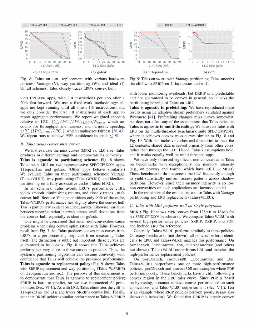
Fig. 8: Talus on LRU replacement with various hardware

policies: Vantage (V), way partitioning (W), and ideal (I).

On all schemes, Talus closely traces LRU’s convex hull.

SPEC CPU2006 apps, with 1 B instructions per app after a

20 B fast-forward. We use a fixed-work methodology: all

apps are kept running until all finish 1 B instructions, and

we only consider the first 1 B instructions of each app to

report aggregate performance. We report weighted speedup

relative to LRU, (∑

i IPCi/IPCi,LRU )/Napps, which ac-

counts for throughput and fairness; and harmonic speedup,

1/∑

i(IPCi,LRU/IPCi), which emphasizes fairness [36, 43].

We repeat runs to achieve 95% confidence intervals ≤1%.

B. Talus yields convex miss curves

We first evaluate the miss curves (MPKI vs. LLC size) Talus

produces in different settings and demonstrate its convexity.

Talus is agnostic to partitioning scheme: Fig. 8 shows

Talus with LRU on two representative SPEC CPU2006 apps,

libquantum and gobmk. (Other apps behave similarly.)

We evaluate Talus on three partitioning schemes: Vantage

(Talus+V/LRU), way partitioning (Talus+W/LRU), and idealized

partitioning on a fully-associative cache (Talus+I/LRU).

In all schemes, Talus avoids LRU’s performance cliffs,

yields smooth, diminishing returns, and closely traces LRU’s

convex hull. Because Vantage partitions only 90% of the cache,

Talus+V/LRU’s performance lies slightly above the convex hull.

This is particularly evident on libquantum. Likewise, variation

between reconfiguration intervals causes small deviations from

the convex hull, especially evident on gobmk.

One might be concerned that small non-convexities cause

problems when using convex optimization with Talus. However,

recall from Fig. 7 that Talus produces convex miss curves from

LRU’s in a pre-processing step, not from measuring Talus

itself. The distinction is subtle but important: these curves are

guaranteed to be convex; Fig. 8 shows that Talus achieves

performance very close to these curves in practice. Thus, the

system’s partitioning algorithm can assume convexity with

confidence that Talus will achieve the promised performance.

Talus is agnostic to replacement policy: Fig. 9 shows Talus

with SRRIP replacement and way partitioning (Talus+W/SRRIP)

on libquantum and mcf. The purpose of this experiment is

to demonstrate that Talus is agnostic to replacement policy;

SRRIP is hard to predict, so we use impractical 64-point

monitors (Sec. VI-C). As with LRU, Talus eliminates the cliff in

libquantum and lbm and traces SRRIP’s convex hull. Finally,

note that DRRIP achieves similar performance to Talus+V/SRRIP

SRRIP Talus +W/SRRIP

0 5 10 15 20 25 30 35 40

LLC Size (MB)

0

5

10

15

20

25

30

35

MP

KI

(a) libquantum

0 2 4 6 8 10 12 14 16

LLC Size (MB)

0

5

10

15

MP

KI

(b) mcf

Fig. 9: Talus on SRRIP with Vantage partitioning. Talus smooths

the cliff with SRRIP on libquantum and mcf.

with lower monitoring overheads, but DRRIP is unpredictable

and not guaranteed to be convex in general, so it lacks the

partitioning benefits of Talus on LRU.

Talus is agnostic to prefetching: We have reproduced these

results using L2 adaptive stream prefetchers validated against

Westmere [41]. Prefetching changes miss curves somewhat,

but does not affect any of the assumptions that Talus relies on.

Talus is agnostic to multi-threading: We have run Talus with

LRU on the multi-threaded benchmark suite SPEC OMP2012,

where it achieves convex miss curves similar to Fig. 8 and

Fig. 10. With non-inclusive caches and directories to track the

L2 contents, shared data is served primarily from other cores,

rather than through the LLC. Hence, Talus’s assumptions hold,

and it works equally well on multi-threaded apps.

We have only observed significant non-convexities in Talus

on benchmarks with exceptionally low memory intensity

(e.g., on povray and tonto, which have <0.1 L2 MPKI).

These benchmarks do not access the LLC frequently enough

to yield statistically uniform access patterns across shadow

partitions. However, since their memory intensity is so low,

non-convexities on such applications are inconsequential.

In the remainder of the evaluation, we use Talus with Vantage

partitioning and LRU replacement (Talus+V/LRU).

C. Talus with LRU performs well on single programs

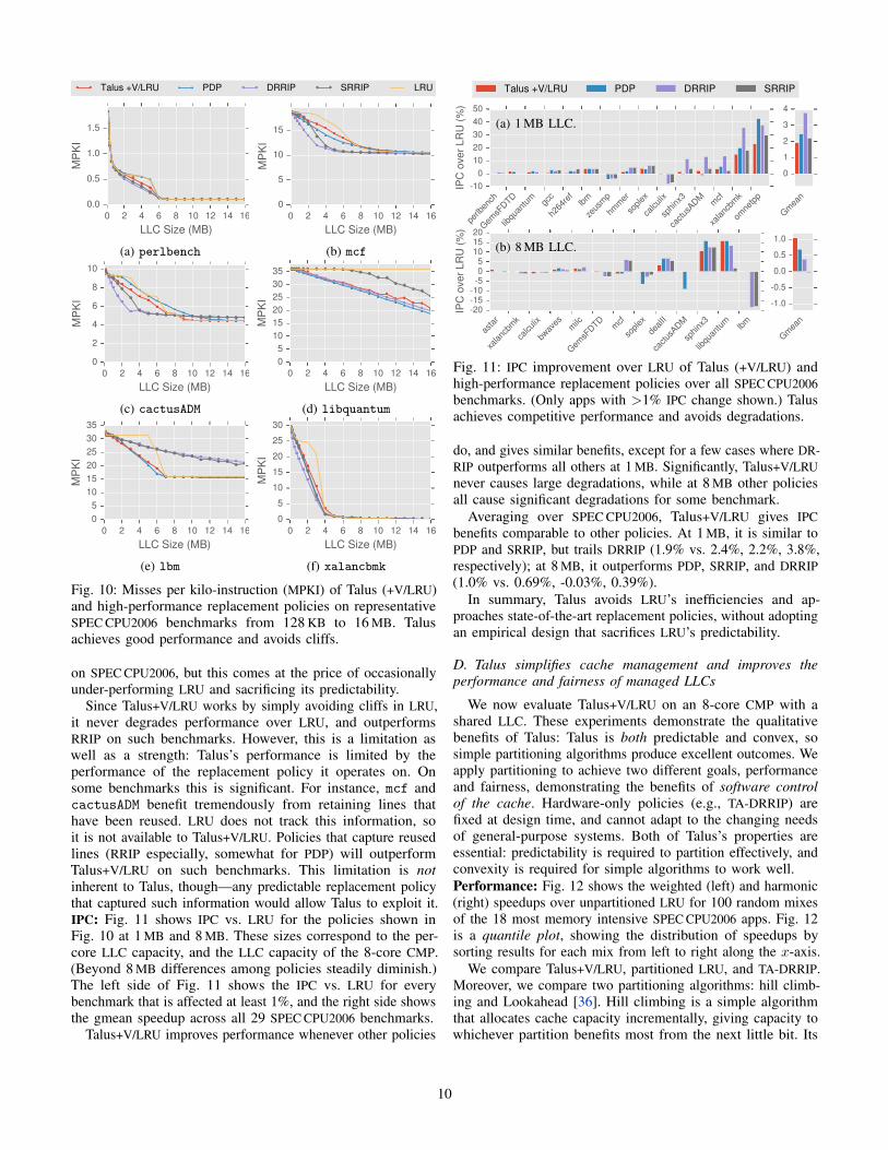
MPKI: Fig. 10 shows MPKI curves from 128 KB to 16 MB for

six SPEC CPU2006 benchmarks. We compare Talus+V/LRU with

several high-performance policies: SRRIP, DRRIP, and PDP,

and include LRU for reference.

Generally, Talus+V/LRU performs similarly to these policies.

On many benchmarks (not shown), all policies perform identi-

cally to LRU, and Talus+V/LRU matches this performance. On

perlbench, libquantum, lbm, and xalancbmk (and others

not shown), Talus+V/LRU outperforms LRU and matches the

high-performance replacement policies.

On perlbench, cactusADM, libquantum, and lbm,

Talus+V/LRU outperforms one or more high-performance

policies. perlbench and cactusADM are examples where PDP

performs poorly. These benchmarks have a cliff following a

convex region in the LRU miss curve. Since PDP is based

on bypassing, it cannot achieve convex performance on such

applications, and Talus+V/LRU outperforms it (Sec. V-C). lbm

is an example where RRIP policies perform poorly (Gems also

shows this behavior). We found that DRRIP is largely convex

9

Talus +V/LRU PDP DRRIP SRRIP LRU

0 2 4 6 8 10 12 14 16

LLC Size (MB)

0.0

0.5

1.0

1.5

MP

KI

(a) perlbench

0 2 4 6 8 10 12 14 16

LLC Size (MB)

0

5

10

15

MP

KI

(b) mcf

0 2 4 6 8 10 12 14 16

LLC Size (MB)

0

2

4

6

8

10

MP

KI

(c) cactusADM

0 2 4 6 8 10 12 14 16

LLC Size (MB)

0

5

10

15

20

25

30

35M

PK

I

(d) libquantum

0 2 4 6 8 10 12 14 16

LLC Size (MB)

0

5

10

15

20

25

30

35

MP

KI

(e) lbm

0 2 4 6 8 10 12 14 16

LLC Size (MB)

0

5

10

15

20

25

30

MP

KI

(f) xalancbmk

Fig. 10: Misses per kilo-instruction (MPKI) of Talus (+V/LRU)

and high-performance replacement policies on representative

SPEC CPU2006 benchmarks from 128 KB to 16 MB. Talus

achieves good performance and avoids cliffs.

on SPEC CPU2006, but this comes at the price of occasionally

under-performing LRU and sacrificing its predictability.

Since Talus+V/LRU works by simply avoiding cliffs in LRU,

it never degrades performance over LRU, and outperforms

RRIP on such benchmarks. However, this is a limitation as

well as a strength: Talus’s performance is limited by the

performance of the replacement policy it operates on. On

some benchmarks this is significant. For instance, mcf and

cactusADM benefit tremendously from retaining lines that

have been reused. LRU does not track this information, so

it is not available to Talus+V/LRU. Policies that capture reused

lines (RRIP especially, somewhat for PDP) will outperform

Talus+V/LRU on such benchmarks. This limitation is not

inherent to Talus, though—any predictable replacement policy

that captured such information would allow Talus to exploit it.

IPC: Fig. 11 shows IPC vs. LRU for the policies shown in

Fig. 10 at 1 MB and 8 MB. These sizes correspond to the per-

core LLC capacity, and the LLC capacity of the 8-core CMP.

(Beyond 8 MB differences among policies steadily diminish.)

The left side of Fig. 11 shows the IPC vs. LRU for every

benchmark that is affected at least 1%, and the right side shows

the gmean speedup across all 29 SPEC CPU2006 benchmarks.

Talus+V/LRU improves performance whenever other policies

Talus +V/LRU PDP DRRIP SRRIP

perlb

ench

Gem

sFDTD

libqu

antu

mgc

c

h264

ref

lbm

zeus

mp

hmm

er

soplex

calculix

sphinx

3

cactus

ADM

mcf

xalanc

bmk

omne

tpp

-10

0

10

20

30

40

50

IPC

over

LR

U (

%)

Gm

ean

0

1

2

3

4

(a) 1 MB LLC.

asta

r

xalanc

bmk

calculix

bwav

esm

ilc

Gem

sFDTD

mcf

soplex

dealII

cactus

ADM

sphinx

3

libqu

antu

mlbm

-20-15-10-505

101520

IPC

over

LR

U (

%)

Gm

ean

-1.0

-0.5

0.0

0.5

1.0(b) 8 MB LLC.

Fig. 11: IPC improvement over LRU of Talus (+V/LRU) and

high-performance replacement policies over all SPEC CPU2006

benchmarks. (Only apps with >1% IPC change shown.) Talus

achieves competitive performance and avoids degradations.

do, and gives similar benefits, except for a few cases where DR-

RIP outperforms all others at 1 MB. Significantly, Talus+V/LRU

never causes large degradations, while at 8 MB other policies

all cause significant degradations for some benchmark.

Averaging over SPEC CPU2006, Talus+V/LRU gives IPC

benefits comparable to other policies. At 1 MB, it is similar to

PDP and SRRIP, but trails DRRIP (1.9% vs. 2.4%, 2.2%, 3.8%,

respectively); at 8 MB, it outperforms PDP, SRRIP, and DRRIP

(1.0% vs. 0.69%, -0.03%, 0.39%).

In summary, Talus avoids LRU’s inefficiencies and ap-

proaches state-of-the-art replacement policies, without adopting

an empirical design that sacrifices LRU’s predictability.

D. Talus simplifies cache management and improves the

performance and fairness of managed LLCs

We now evaluate Talus+V/LRU on an 8-core CMP with a

shared LLC. These experiments demonstrate the qualitative

benefits of Talus: Talus is both predictable and convex, so

simple partitioning algorithms produce excellent outcomes. We

apply partitioning to achieve two different goals, performance

and fairness, demonstrating the benefits of software control

of the cache. Hardware-only policies (e.g., TA-DRRIP) are

fixed at design time, and cannot adapt to the changing needs

of general-purpose systems. Both of Talus’s properties are

essential: predictability is required to partition effectively, and

convexity is required for simple algorithms to work well.

Performance: Fig. 12 shows the weighted (left) and harmonic

(right) speedups over unpartitioned LRU for 100 random mixes

of the 18 most memory intensive SPEC CPU2006 apps. Fig. 12

is a quantile plot, showing the distribution of speedups by

sorting results for each mix from left to right along the x-axis.

We compare Talus+V/LRU, partitioned LRU, and TA-DRRIP.

Moreover, we compare two partitioning algorithms: hill climb-

ing and Lookahead [36]. Hill climbing is a simple algorithm

that allocates cache capacity incrementally, giving capacity to

whichever partition benefits most from the next little bit. Its

10

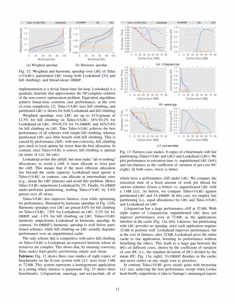
Talus +V/LRU (Hill) Lookahead TA-DRRIP Hill LRU

0 20 40 60 80 100

Workload Mix

1.0

1.1

1.2

1.3

1.4

Weig

hte

d S

peedup

(a) Weighted speedup.

0 20 40 60 80 100

Workload Mix

0.95

1.00

1.05

1.10

1.15

Ha

rmo

nic

Sp

ee

du

p

(b) Harmonic speedup.

Fig. 12: Weighted and harmonic speedup over LRU of Talus

(+V/LRU), partitioned LRU (using both Lookahead [36] and

hill climbing), and thread-aware DRRIP.

implementation is a trivial linear-time for-loop. Lookahead is a

quadratic heuristic that approximates the NP-complete solution

of the non-convex optimization problem. Equivalent algorithms

achieve linear-time common case performance, at the cost

of extra complexity [2]. Talus+V/LRU uses hill climbing, and

partitioned LRU is shown for both Lookahead and hill climbing.

Weighted speedups over LRU are up to 41%/gmean of

12.5% for hill climbing on Talus+V/LRU, 34%/10.2% for

Lookahead on LRU, 39%/6.3% for TA-DRRIP, and 16%/3.8%

for hill climbing on LRU. Thus Talus+V/LRU achieves the best

performance of all schemes with simple hill climbing, whereas

partitioned LRU sees little benefit with hill climbing. This is

caused by performance cliffs: with non-convexity, hill climbing

gets stuck in local optima far worse than the best allocation. In

contrast, since Talus+V/LRU is convex, hill climbing is optimal

(in terms of LLC hit rate).

Lookahead avoids this pitfall, but must make “all-or-nothing”

allocations: to avoid a cliff, it must allocate to sizes past

the cliff. This means that if the most efficient allocation

lies beyond the cache capacity, Lookahead must ignore it.

Talus+V/LRU, in contrast, can allocate at intermediate sizes

(e.g., along the LRU plateau) and avoid this problem. Hence

Talus+V/LRU outperforms Lookahead by 2%. Finally, TA-DRRIP

under-performs partitioning, trailing Talus+V/LRU by 5.6%

gmean over all mixes.

Talus+V/LRU also improves fairness, even while optimizing

for performance, illustrated by harmonic speedups in Fig. 12(b).

Harmonic speedups over LRU are gmean 8.0% for hill climbing

on Talus+V/LRU, 7.8% for Lookahead on LRU, 5.2% for TA-

DRRIP, and -1.8% for hill climbing on LRU. Talus+V/LRU

modestly outperforms Lookahead in harmonic speedup. In

contrast, TA-DRRIP’s harmonic speedup is well below parti-

tioned schemes, while hill climbing on LRU actually degrades

performance over an unpartitioned cache.

The only scheme that is competitive with naıve hill climbing

on Talus+V/LRU is Lookahead, an expensive heuristic whose al-

ternatives are complex. This shows that, by ensuring convexity,

Talus makes high-quality partitioning simple and cheap.

Fairness: Fig. 13 shows three case studies of eight copies of

benchmarks on the 8-core system with LLC sizes from 1 MB

to 72 MB. This system represents a homogeneous application

in a setting where fairness is paramount. Fig. 13 shows three

benchmarks: libquantum, omnetpp, and xalancbmk, all of

Talus +V/LRU (Fair) Lookahead TA-DRRIP Fair LRU

0 10 20 30 40 50 60 70 80

Cache Size (MB)

0.820.840.860.880.900.920.940.960.981.00

Exe

cu

tio

n T

ime

0 10 20 30 40 50 60 70 80

Cache Size (MB)

0.0

0.2

0.4

0.6

0.8

1.0

Co

V o

f C

ore

IP

C

(a) libquantum.

0 10 20 30 40 50 60 70 80

Cache Size (MB)

0.10.20.30.40.50.60.70.80.91.0

Exe

cu

tio

n T

ime

0 10 20 30 40 50 60 70 80

Cache Size (MB)

0.0

0.2

0.4

0.6

0.8

1.0

1.2

Co

V o

f C

ore

IP

C

(b) omnetpp.

0 10 20 30 40 50 60 70 80

Cache Size (MB)

0.2

0.4

0.6

0.8

1.0

Exe

cu

tio

n T

ime

0 10 20 30 40 50 60 70 80

Cache Size (MB)

0.0

0.1

0.2

0.3

0.4

0.5

0.6

0.7

0.8

Co

V o

f C

ore

IP

C

(c) xalancbmk.

Fig. 13: Fairness case studies: 8 copies of a benchmark with fair

partitioning (Talus+V/LRU and LRU) and Lookahead (LRU). We

plot performance as execution time vs. unpartitioned LRU (left);

and (un-)fairness as the coefficient of variation of per-core IPC

(right). In both cases, lower is better.

which have a performance cliff under LRU. We compare the

execution time of a fixed amount of work per thread for

various schemes (lower is better) vs. unpartitioned LRU with

a 1 MB LLC. As before, we compare Talus+V/LRU against

partitioned LRU and TA-DRRIP. In this case, we employ fair

partitioning (i.e., equal allocations) for LRU and Talus+V/LRU,

and Lookahead on LRU.libquantum has a large performance cliff at 32 MB. With

eight copies of libquantum, unpartitioned LRU does not

improve performance even at 72 MB, as the applications

interfere in the cache (Fig. 13a, left). Likewise, fair partitioning

with LRU provides no speedup, since each application requires

32 MB to perform well. Lookahead improves performance, but

at the cost of fairness: after 32 MB, Lookahead gives the entire

cache to one application, boosting its performance without

benefiting the others. This leads to a large gap between the

IPCs of different cores, shown by the coefficient of variation

of core IPC (i.e., the standard deviation of IPCs divided by the

mean IPC; Fig. 13a, right). TA-DRRIP thrashes in the cache,

and never settles on any single core to prioritize.In contrast, Talus+V/LRU gives steady gains with increasing

LLC size, achieving the best performance except when Looka-

head briefly outperforms it (due to Vantage’s unmanaged region;

11

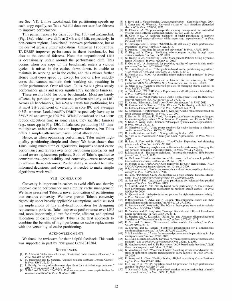
see Sec. VI). Unlike Lookahead, fair partitioning speeds up

each copy equally, so Talus+V/LRU does not sacrifice fairness

to improve performance.This pattern repeats for omnetpp (Fig. 13b) and xalancbmk

(Fig. 13c), which have cliffs at 2 MB and 6 MB, respectively. In

non-convex regions, Lookahead improves performance, but at

the cost of grossly unfair allocations. Unlike in libquantum,

TA-DRRIP improves performance in these benchmarks, but

also at the cost of fairness. Note that unpartitioned LRU

is occasionally unfair around the performance cliff. This

occurs when one copy of the benchmark enters a vicious

cycle: it misses in the cache, slows down, is unable to

maintain its working set in the cache, and thus misses further.

Hence most cores speed up, except for one or a few unlucky

cores that cannot maintain their working set, resulting in

unfair performance. Over all sizes, Talus+V/LRU gives steady

performance gains and never significantly sacrifices fairness.These results hold for other benchmarks. Most are barely

affected by partitioning scheme and perform similarly to LRU.

Across all benchmarks, Talus+V/LRU with fair partitioning has

at most 2% coefficient of variation in core IPC and averages

0.3%, whereas Lookahead/TA-DRRIP respectively have up to

85%/51% and average 10%/5%. While Lookahead or TA-DRRIP

reduce execution time in some cases, they sacrifice fairness

(e.g., omnetpp in Fig. 13b). Imbalanced partitioning [35] time-

multiplexes unfair allocations to improve fairness, but Talus

offers a simpler alternative: naıve, equal allocations.Hence, as when optimizing performance, Talus makes high-

quality partitioning simple and cheap. We have shown that

Talus, using much simpler algorithms, improves shared cache

performance and fairness over prior partitioning approaches and

thread-aware replacement policies. Both of Talus’s qualitative

contributions—predictability and convexity—were necessary

to achieve these outcomes: Predictability is needed to make

informed decisions, and convexity is needed to make simple

algorithms work well.

VIII. CONCLUSION

Convexity is important in caches to avoid cliffs and thereby

improve cache performance and simplify cache management.

We have presented Talus, a novel application of partitioning

that ensures convexity. We have proven Talus’s convexity

rigorously under broadly applicable assumptions, and discussed

the implications of this analytical foundation for designing

replacement policies. Talus improves performance over LRU

and, more importantly, allows for simple, efficient, and optimal

allocation of cache capacity. Talus is the first approach to

combine the benefits of high-performance cache replacement

with the versatility of cache partitioning.

ACKNOWLEDGMENTS

We thank the reviewers for their helpful feedback. This work

was supported in part by NSF grant CCF-1318384.

REFERENCES

[1] D. Albonesi, “Selective cache ways: On-demand cache resource allocation,” inProc. MICRO-32, 1999.

[2] N. Beckmann and D. Sanchez, “Jigsaw: Scalable Software-Defined Caches,”in Proc. PACT-22, 2013.

[3] L. Belady, “A study of replacement algorithms for a virtual-storage computer,”IBM Systems journal, vol. 5, no. 2, 1966.

[4] S. Bird and B. Smith, “PACORA: Performance aware convex optimization forresource allocation,” in Proc. HotPar-3, 2011.

[5] S. Boyd and L. Vandenberghe, Convex optimization. Cambridge Press, 2004.[6] J. Carter and M. Wegman, “Universal classes of hash functions (Extended

abstract),” in Proc. STOC-9, 1977.[7] D. Chiou et al., “Application-specific memory management for embedded

systems using software-controlled caches,” in Proc. DAC-37, 2000.[8] H. Cook et al., “A hardware evaluation of cache partitioning to improve

utilization and energy-efficiency while preserving responsiveness,” in Proc.ISCA-40, 2013.

[9] C. Curtsinger and E. Berger, “STABILIZER: statistically sound performanceevaluation,” in Proc. ASPLOS-XVIII, 2013.

[10] P. Denning, “Thrashing: Its causes and prevention,” in Proc. AFIPS, 1968.[11] C. Ding and Y. Zhong, “Predicting whole-program locality through reuse

distance analysis,” in Proc. PLDI, 2003.[12] N. Duong et al., “Improving Cache Management Policies Using Dynamic

Reuse Distances,” in Proc. MICRO-45, 2012.[13] F. Guo et al., “A framework for providing quality of service in chip multi-

processors,” in Proc. MICRO-40, 2007.[14] W. Hasenplaugh et al., “The gradient-based cache partitioning algorithm,”

ACM Trans. on Arch. and Code Opt., vol. 8, no. 4, 2012.[15] R. Hundt et al., “MAO–An extensible micro-architectural optimizer,” in Proc.

CGO, 2011.[16] R. Iyer et al., “QoS policies and architecture for cache/memory in CMP

platforms,” ACM SIGMETRICS Perf. Eval. Review, vol. 35, no. 1, 2007.[17] A. Jaleel et al., “Adaptive insertion policies for managing shared caches,” in

Proc. PACT-17, 2008.[18] A. Jaleel et al., “CRUISE: Cache Replacement and Utility-Aware Scheduling,”

in Proc. ASPLOS-XVII, 2012.[19] A. Jaleel et al., “High Performance Cache Replacement Using Re-Reference

Interval Prediction (RRIP),” in Proc. ISCA-37, 2010.[20] D. Kanter, “Silvermont, Intel’s Low Power Architecture,” in RWT, 2013.[21] H. Kasture and D. Sanchez, “Ubik: Efficient Cache Sharing with Strict QoS

for Latency-Critical Workloads,” in Proc. ASPLOS-XIX, 2014.[22] G. Keramidas, P. Petoumenos, and S. Kaxiras, “Cache replacement based on

reuse-distance prediction,” in Proc. ICCD, 2007.[23] R. Kessler, M. Hill, and D. Wood, “A comparison of trace-sampling techniques

for multi-megabyte caches,” IEEE Trans. on Computers, vol. 43, no. 6, 1994.[24] S. Khan, Z. Wang, and D. Jimenez, “Decoupled dynamic cache segmentation,”

in Proc. HPCA-18, 2012.[25] M. Kharbutli et al., “Using prime numbers for cache indexing to eliminate

conflict misses,” in Proc. HPCA-10, 2004.[26] D. Knuth, Axioms and hulls. Springer-Verlag Berlin, 1992.[27] N. Kurd et al., “Westmere: A family of 32nm IA processors,” in Proc. ISSCC,

2010.[28] H. Lee, S. Cho, and B. Childers, “CloudCache: Expanding and shrinking

private caches,” in Proc. HPCA-17, 2011.[29] J. Lin et al., “Gaining insights into multicore cache partitioning: Bridging the

gap between simulation and real systems,” in Proc. HPCA-14, 2008.[30] R. Mattson et al., “Evaluation techniques for storage hierarchies,” IBM Systems

journal, vol. 9, no. 2, 1970.[31] A. Melkman, “On-line construction of the convex hull of a simple polyline,”

Information Processing Letters, vol. 25, no. 1, 1987.[32] M. Moreto et al., “FlexDCP: A QoS framework for CMP architectures,” ACM

SIGOPS Operating Systems Review, vol. 43, no. 2, 2009.[33] T. Mytkowicz et al., “Producing wrong data without doing anything obviously

wrong!” in Proc. ASPLOS-XIV, 2009.[34] D. Page, “Partitioned Cache Architecture as a Side-Channel Defence Mecha-

nism,” IACR Cryptology ePrint archive, no. 2005/280, 2005.[35] A. Pan and V. Pai, “Imbalanced cache partitioning for balanced data-parallel

programs,” in Proc. MICRO-46, 2013.[36] M. Qureshi and Y. Patt, “Utility-based cache partitioning: A low-overhead,

high-performance, runtime mechanism to partition shared caches,” in Proc.MICRO-39, 2006.

[37] M. Qureshi et al., “Adaptive insertion policies for high performance caching,”in Proc. ISCA-34, 2007.

[38] P. Ranganathan, S. Adve, and N. Jouppi, “Reconfigurable caches and theirapplication to media processing,” in Proc. ISCA-27, 2000.

[39] D. Sanchez and C. Kozyrakis, “The ZCache: Decoupling Ways and Associativ-ity,” in Proc. MICRO-43, 2010.

[40] D. Sanchez and C. Kozyrakis, “Vantage: Scalable and Efficient Fine-GrainCache Partitioning,” in Proc. ISCA-38, 2011.

[41] D. Sanchez and C. Kozyrakis, “ZSim: Fast and Accurate MicroarchitecturalSimulation of Thousand-Core Systems,” in Proc. ISCA-40, 2013.

[42] R. Sen and D. Wood, “Reuse-based online models for caches,” in Proc.SIGMETRICS, 2013.

[43] A. Snavely and D. Tullsen, “Symbiotic jobscheduling for a simultaneousmultithreading processor,” in Proc. ASPLOS-IX, 2000.

[44] S. Srikantaiah et al., “A case for integrated processor-cache partitioning in chipmultiprocessors,” in Proc. SC09, 2009.

[45] G. E. Suh, L. Rudolph, and S. Devadas, “Dynamic partitioning of shared cachememory,” The Journal of Supercomputing, vol. 28, no. 1, 2004.

[46] H. Vandierendonck and K. De Bosschere, “XOR-based hash functions,” IEEETrans. on Computers, vol. 54, no. 7, 2005.

[47] K. Varadarajan et al., “Molecular Caches: A caching structure for dynamic cre-ation of application-specific Heterogeneous cache regions,” in Proc. MICRO-39, 2006.

[48] R. Wang and L. Chen, “Futility Scaling: High-Associativity Cache Partition-ing,” in Proc. MICRO-47, 2014.

[49] C.-J. Wu et al., “SHiP: Signature-based hit predictor for high performancecaching,” in Proc. MICRO-44, 2011.

[50] Y. Xie and G. Loh, “PIPP: promotion/insertion pseudo-partitioning of multi-core shared caches,” in Proc. ISCA-36, 2009.

12