Embed Size (px)
Citation preview

Appendix B
Quantification Methods for Tree Planting Projects
Version 9
February 7, 2021

City Forest Credits – Appendix B February 2021
Urban Forest Carbon Registry, City Forest Credits, a 501(c)(3) non-profit
organization
999 Third Ave. #4600
Seattle, WA 98104
(206) 623-1823
Copyright © 2016-2021 Urban Forest Carbon Registry and City Forest Credits. All rights
reserved.

City Forest Credits – Appendix B February 2021
3
This Appendix B on Quantification for Tree Planting Projects consists of two Parts.
Part 1 contains a description of the science and methods underlying quantification
of CO2 and co-benefits in city trees.
Part 2 contains a Summary of Quantification Steps, followed by a longer section
entitled Quantification Methods and Examples, which provides a more detailed
walk-though of quantification methods using examples.
The principal author of this Appendix B on Quantification is Dr. E.G. McPherson. Dr.
McPherson also led the science teams that developed quantification methods for
the State of California Air Resources Board Urban Forest Carbon Protocol in 2011
and the Climate Action Reserve Urban Forest Protocols in 2014.
Note that quantification methods for Tree Preservation Projects, as distinct
from Tree Planting Projects, are contained within the Tree Preservation
Protocol.
Part 1
Quantifying Carbon Dioxide Storage and Co-Benefits for Urban
Tree Planting Projects
Introduction
Ecoservices provided by trees to human beneficiaries are classified according to
their spatial scale as global and local (Costanza 2008) (citations in Part 1 are listed in
References at page 16). Removal of carbon dioxide (CO2) from the atmosphere by
urban forests is global because the atmosphere is so well-mixed it does not matter
where the trees are located. The effects of urban forests on building energy use is a
local-scale service because it depends on the proximity of trees to buildings. To
quantify these and other ecoservices City Forest Credits (CFC) has relied on peer-
reviewed research that has combined measurements and modeling of urban tree
biomass, and effects of trees on building energy use, rainfall interception, and air
quality. CFC has used the most current science available on urban tree growth in its
estimates of CO2 storage (McPherson et al., 2016a). CFC’s quantification tools

City Forest Credits – Appendix B February 2021
4
provide estimates of co-benefits after 25 years in Resource Units (i.e., kWh of
electricity saved) and dollars per year. Values for co-benefits are first-order
approximations extracted from the i-Tree Streets (i-Tree Eco) datasets for each of
the 16 U.S. reference cities/climate zones (https://www.itreetools.org/tools/i-tree-
eco) (Maco and McPherson, 2003). Modeling approaches and error estimates
associated with quantification of CO2 storage and co-benefits have been
documented in numerous publications (see References below) and are summarized
here.
Carbon Dioxide Storage
There are three different methods for quantifying carbon dioxide (CO2) storage in
urban forest carbon projects:
• Single Tree Method - planted trees are scattered among many existing trees,
as in street, yard, some parks, and school plantings, individual trees are
tracked and randomly sampled
• Clustered Parks Planting Method - planted trees are relatively contiguous in
park-like settings and change in canopy is tracked
• Canopy Method – trees are planted very close together, often but not
required to be in riparian areas, significant mortality is expected, and change
in canopy is tracked. The two main goals are to create a forest ecosystem
and generate canopy
• Area Reforestation Method – large areas are planted to generate a forest
ecosystem, for example converting from agriculture and in upland areas.
This quantification method is under development
In all cases, the estimated amount of CO2 stored 25-years after planting is
calculated. The forecasted amount of CO2 stored during this time is the value from
which the Registry issues credits in the amounts of 10%, 40% and 30% at Years 1, 4,
and 6 after planting, respectively. A 20% mortality deduction is applied before
calculation of Year 1 Credits in the Single Tree and Clustered Parks Planting
Methods. A 5% buffer pool deduction is applied in all three methods before
calculation of any crediting, with these funds going into a program-wide pool to
insure against catastrophic loss of trees. At the end of the project, in year 25,
Operators will receive credits for all CO2 stored, minus credits already issued.

City Forest Credits – Appendix B February 2021
5
In the Single Tree Method, the amount of CO2 stored in project trees 25-years after
planting is calculated as the product of tree numbers and the 25-year CO2 index
(kg/tree) for each tree-type (e.g., Broadleaf Deciduous Large = BDL). The Registry
requires the user to apply a 20% tree mortality deduction before calculation of Year
1 Credits. Year 4 and Year 6 Credits depend on sampling and mortality data. A 5%
buffer pool deduction is applied as well before calculation at any stage.
In the Clustered Parks Planting Method, the amount of CO2 stored after 25-years by
planted project trees is based on the anticipated amount of tree canopy area (TC).
Because different tree-types store different amounts of CO2 based on their size and
wood density, TC is weighted based on species mix. The estimated amount of TC
area occupied by each tree-type is the product of the total TC and each tree-type’s
percentage TC. This calculation distributes the TC area among tree-types based on
the percentage of trees planted and each tree-type’s crown projection area.
Subsequent calculations reduce the amount of CO2 estimated to be stored after 25
years based on the 20% anticipated mortality rate and the 5% buffer pool
deduction.
In the Canopy Method, the forecasted amount of CO2 stored at 25-years is the
product of the amount of TC and the CO2 Index (CI, t CO2 per acre). This approach
recognizes that forest dynamics for riparian projects are different than for park
projects. In many cases, native species are planted close together and early
competition results in high mortality and rapid canopy closure. Unlike urban park
plantings, substantial amounts of carbon can be stored in the riparian understory
vegetation and forest floor. To provide an accurate and complete accounting, we
use the USDA Forest Service General Technical Report NE-343, with biometric data
for 51 forest ecosystems derived from U.S. Forest Inventory and Assessment plots
(Smith et al., 2006). The tables provide carbon stored per hectare for each of six
carbon pools as a function of stand age. We use values for 25-year old stands that
account for carbon in down dead wood and forest floor material, as well as the
understory vegetation and soil. If local plot data are provided, values for live wood,
dead standing and dead down wood are adjusted following guidance in GTR NE-
343. More information on methods used to prepare the tables and make
adjustments can be found in Smith et al., 2006. See Attachment A at the end of this
Appendix for more information on the Canopy Method.

City Forest Credits – Appendix B February 2021
6
Source Materials for Single Tree Method and Clustered Parks
Planting Methods
Estimates of stored (amount accumulated over many years) and sequestered CO2
(i.e., net amount stored by tree growth over one year) are based on the U.S. Forest
Service’s recently published technical manual and the extensive Urban Tree
Database (UTD), which catalogs urban trees with their projected growth tailored to
specific geographic regions (McPherson et al. 2016a, b). The products are a
culmination of 14 years of work, analyzing more than 14,000 trees across the
United States. Whereas prior growth models typically featured only a few species
specific to a given city or region, the newly released database features 171 distinct
species across 16 U.S. climate zones. The trees studied also spanned a range of
ages with data collected from a consistent set of measurements. Advances in
statistical modeling have given the projected growth dimensions a level of accuracy
never before seen. Moving beyond just calculating a tree’s diameter or age to
determine expected growth, the research incorporates 365 sets of tree growth
equations to project growth.
Users select their climate zone from the 16 U.S. climate zones (Fig. 1). Calculations
of CO2 stored are for a representative species for each tree-type that was one of
the predominant street tree species per reference city (Peper et al., 2001). The
“Reference city” refers to the city selected for intensive study within each climate
zone (McPherson, 2010). About 20 of the most abundant species were selected for
sampling in each reference city. The sample was stratified into nine diameter at
breast height (DBH) classes (0 to 7.6, 7.6 to 15.2, 15.2 to 30.5, 30.5 to 45.7, 45.7 to
61.0, 61.0 to 76.2, 76.2 to 91.4, 91.4 to 106.7, and >106.7 cm). Typically 10 to 15
trees per DBH class were randomly chosen. Data were collected for 16 to 74 trees
in total from each species. Measurements included: species name, age, DBH [to the
nearest 0.1 cm (0.39 in)], tree height [to the nearest 0.5 m (1.64 ft.)], crown height
[to the nearest 0.5 m (1.64 ft.)], and crown diameter in two directions [parallel and
perpendicular to nearest street to the nearest 0.5 m (1.64 ft.)]. Tree age was
determined from local residents, the city’s urban forester, street and home
construction dates, historical planting records, and aerial and historical photos.

City Forest Credits – Appendix B February 2021
7
Fig. 1. Climate zones of the United States and Puerto Rico were aggregated from 45
Sunset climate zones into 16 zones. Each zone has a reference city where tree data
were collected. Sacramento, California was added as a second reference city (with
Modesto) to the Inland Valleys zone. Zones for Alaska, Puerto Rico and Hawaii are
shown in the insets (map courtesy of Pacific Southwest Research Station).
Species Assignment by Tree-Type
Representative species for each tree-type in the South climate zone (reference city
is Charlotte, NC) are shown in Table 1. They were chosen because extensive
measurements were taken on them to generate growth equations, and their
mature size and form was deemed typical of other trees in that tree-type.
Representative species were not available for some tree-types because none were
measured. In that case, a species of similar mature size and form from the same
climate zone was selected, or one from another climate zone was selected. For
City Forest Credits – Appendix B February 2021
8
example, no Broadleaf Evergreen Large (BEL) species was measured in the South
reference city. Because of its large mature size, Quercus nigra was selected to
represent the BEL tree-type, although it is deciduous for a short time. Pinus
contorta, which was measured in the PNW climate zone, was selected for the CES
tree-type, because no CES species was measured in the South.
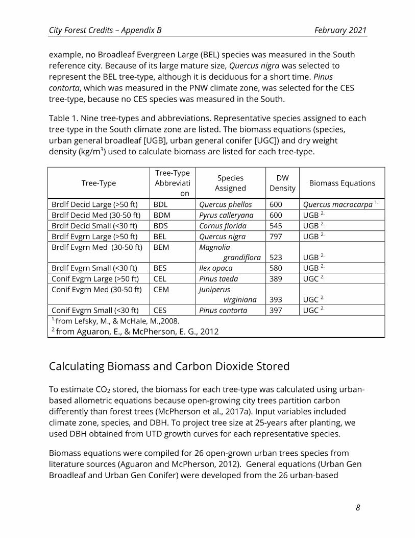
Table 1. Nine tree-types and abbreviations. Representative species assigned to each
tree-type in the South climate zone are listed. The biomass equations (species,
urban general broadleaf [UGB], urban general conifer [UGC]) and dry weight
density (kg/m3) used to calculate biomass are listed for each tree-type.
Tree-Type
Tree-Type
Abbreviati
on
Species
Assigned
DW
Density Biomass Equations
Brdlf Decid Large (>50 ft) BDL Quercus phellos 600 Quercus macrocarpa 1.
Brdlf Decid Med (30-50 ft) BDM Pyrus calleryana 600 UGB 2.
Brdlf Decid Small (<30 ft) BDS Cornus florida 545 UGB 2.
Brdlf Evgrn Large (>50 ft) BEL Quercus nigra 797 UGB 2.
Brdlf Evgrn Med (30-50 ft) BEM Magnolia
grandiflora 523 UGB 2.
Brdlf Evgrn Small (<30 ft) BES Ilex opaca 580 UGB 2.
Conif Evgrn Large (>50 ft) CEL Pinus taeda 389 UGC 2.
Conif Evgrn Med (30-50 ft) CEM Juniperus
virginiana 393 UGC 2.
Conif Evgrn Small (<30 ft) CES Pinus contorta 397 UGC 2. 1.from Lefsky, M., & McHale, M.,2008. 2 from Aguaron, E., & McPherson, E. G., 2012
Calculating Biomass and Carbon Dioxide Stored
To estimate CO2 stored, the biomass for each tree-type was calculated using urban-
based allometric equations because open-growing city trees partition carbon
differently than forest trees (McPherson et al., 2017a). Input variables included
climate zone, species, and DBH. To project tree size at 25-years after planting, we
used DBH obtained from UTD growth curves for each representative species.
Biomass equations were compiled for 26 open-grown urban trees species from
literature sources (Aguaron and McPherson, 2012). General equations (Urban Gen
Broadleaf and Urban Gen Conifer) were developed from the 26 urban-based

City Forest Credits – Appendix B February 2021
9
equations that were species specific (McPherson et al., 2016a). These equations
were used if the species of interest could not be matched taxonomically or through
wood form to one of the urban species with a biomass equation. Hence, urban
general equations were an alternative to applying species-specific equations
because many species did not have an equation.
These allometric equations yielded aboveground wood volume. Species-specific dry
weight (DW) density factors (Table 1) were used to convert green volume into dry
weight (7a). The urban general equations required looking up a dry weight density
factor (in Jenkins et al. 2004 first, but if not available then the Global Wood Density
Database). The amount of belowground biomass in roots of urban trees is not well
researched. This work assumed that root biomass was 28% of total tree biomass
(Cairns et al., 1997; Husch et al., 2003; Wenger, 1984). Wood volume (dry weight)
was converted to C by multiplying by the constant 0.50 (Leith, 1975), and C was
converted to CO2 by multiplying by 3.667.
Error Estimates and Limitations
The lack of biometric data from the field remains a serious limitation to our ability
to calibrate biomass equations and assign error estimates for urban trees.
Differences between modeled and actual tree growth adds uncertainty to CO2
sequestration estimates. Species assignment errors result from matching species
planted with the tree-type used for biomass and growth calculations. The
magnitude of this error depends on the goodness of fit in terms of matching size
and growth rate. In previous urban studies the prediction bias for estimates of CO2
storage ranged from -9% to +15%, with inaccuracies as much as 51% RMSE
(Timilsina et al., 2014). Hence, a conservative estimate of error of ± 20% can be
applied to estimates of total CO2 stored as an indicator of precision.
It should be noted that estimates of CO2 stored using the Tree Canopy Approach
have several limitations that may reduce their accuracy. They rely on allometric
relationships for open-growing trees, so storage estimates may not be as accurate
when trees are closely spaced. Also, they assume that the distribution of tree
canopy cover among tree-types remains constant, when in fact mortality may afflict
certain species more than others. For these reasons, periodic “truing-up” of
estimates by field sampling is suggested.

City Forest Credits – Appendix B February 2021
10
Co-Benefit: Energy Savings
Trees and forests can offer energy savings in two important ways. In warmer
climates or hotter months, trees can reduce air conditioning bills by keeping
buildings cooler through reducing regional air temperatures and offering shade. In
colder climates or cooler months, trees can confer savings on the fuel needed to
heat buildings by reducing the amount of cold winds that can strip away heat.
Energy conservation by trees is important because building energy use is a major
contributor to greenhouse gas emissions. Oil or gas furnaces and most forms of
electricity generation produce CO2 and other pollutants as by-products. Reducing
the amount of energy consumed by buildings in urban areas is one of the most
effective methods of combatting climate change. Energy consumption is also a
costly burden on many low-income families, especially during mid-summer or mid-
winter. Furthermore, electricity consumption during mid-summer can sometimes
over-extend local power grids leading to rolling brownouts and other problems.
Energy savings are calculated through numerical models and simulations built from
observational data on proximity of trees to buildings, tree shapes, tree sizes,
building age classes, and meteorological data from McPherson et al. (2017) and
McPherson and Simpson (2003). The main parameters affecting the overall amount
of energy savings are crown shape, building proximity, azimuth, local climate, and
season. Shading effects are based on the distribution of street trees with respect to
buildings recorded from aerial photographs for each reference city (McPherson and
Simpson, 2003). If a sampled tree was located within 18 m of a conditioned
building, information on its distance and compass bearing relative to a building,
building age class (which influences energy use) and types of heating and cooling
equipment were collected and used as inputs to calculate effects of shade on
annual heating and cooling energy effects. Because these distributions were unique
to each city, energy values are considered first-order approximations.
In addition to localized shade effects, which were assumed to accrue only to trees
within 18 m of a building, lowered air temperatures and windspeeds from
increased neighborhood tree cover (referred to as climate effects) can produce a
net decrease in demand for winter heating and summer cooling (reduced wind
speeds by themselves may increase or decrease cooling demand, depending on the
circumstances). Climate effects on energy use, air temperature, and wind speed, as
a function of neighborhood canopy cover, were estimated from published values
for each reference city. The percentages of canopy cover increase were calculated
for 20-year-old large, medium, and small trees, based on their crown projection

City Forest Credits – Appendix B February 2021
11
areas and effective lot size (actual lot size plus a portion of adjacent street and
other rights-of-way) of 10,000 ft2 (929 m2), and one tree on average was assumed
per lot. Climate effects were estimated by simulating effects of wind and air-
temperature reductions on building energy use.
In the case of urban Tree Preservation Projects, trees may not be close enough to
buildings to provide shading effects, but they may influence neighborhood climate.
Because these effects are highly site-specific, we conservatively apply an 80%
reduction to the energy effects of trees for Preservation Projects.
Energy savings are calculated as a real-dollar amount. This is calculated by applying
overall reductions in oil and gas usage or electricity usage to the regional cost of oil
and gas or electricity for residential customers. Colder regions tend to see larger
savings in heating and warmer regions tend to see larger savings in cooling.
Error Estimates and Limitations
Formulaic errors occur in modeling of energy effects. For example, relations
between different levels of tree canopy cover and summertime air temperatures
are not well-researched. Another source of error stems from differences between
the airport climate data (i.e., Los Angeles International Airport) used to model
energy effects and the actual climate of the study area (i.e., Los Angeles urban
area). Because of the uncertainty associated with modeling effects of trees on
building energy use, energy estimates may be accurate within ± 25 percent
(Hildebrandt & Sarkovich, 1998).
Co-Benefit: CO2 Avoided
Energy savings result in reduced emissions of CO2 and criteria air pollutants
(volatile organic hydrocarbons [VOCs], NO2, SO2, PM10) from power plants and
space-heating equipment. Cooling savings reduce emissions from power plants
that produce electricity, the amount depending on the fuel mix. Electricity
emissions reductions were based on the fuel mixes and emission factors for each
utility in the 16 reference cities/climate zones across the U.S. The dollar values of
electrical energy and natural gas were based on retail residential electricity and
natural gas prices obtained from each utility. Utility-specific emission factors, fuel
prices and other data are available in the Community Tree Guides for each region

City Forest Credits – Appendix B February 2021
12
(https://www.fs.fed.us/psw/topics/urban_forestry/products/tree_guides.shtml). To
convert the amount of CO2 avoided to a dollar amount in the spreadsheet tools,
City Forest Credits uses the price of $20 per metric ton of CO2.
Error Estimates and Limitations
Estimates of avoided CO2 emissions have the same uncertainties that are
associated with modeling effects of trees on building energy use. Also, utility-
specific emission factors are changing as many utilities incorporate renewable fuels
sources into their portfolios. Values reported in CFC tools may overestimate actual
benefits in areas where emission factors have become lower.
Co-Benefit: Rainfall Interception
Forest canopies normally intercept 10-40% of rainfall before it hits the ground,
thereby reducing stormwater runoff. The large amount of water that a tree crown
can capture during a rainfall event makes tree planting a best management practice
for urban stormwater control.
City Forest Credits uses a numerical interception model to calculate the amount of
annual rainfall intercepted by trees, as well as throughfall and stem flow (Xiao et al.,
2000). This model uses species-specific leaf surface areas and other parameters
from the Urban Tree Database. For example, deciduous trees in climate zones with
longer “in-leaf” seasons will tend to intercept more rainfall than similar species in
colder areas shorter foliation periods. Model results were compared to observed
patterns of rainfall interception and found to be accurate. This method quantifies
only the amount of rainfall intercepted by the tree crown, and does not incorporate
surface and subsurface effects on overland flow.
The rainfall interception benefit was priced by estimating costs of controlling
stormwater runoff. Water quality and/or flood control costs were calculated per
unit volume of runoff controlled and this price was multiplied by the amount of
rainfall intercepted annually.

City Forest Credits – Appendix B February 2021
13
Error Estimates and Limitations
Estimates of rainfall interception are sensitive to uncertainties regarding rainfall
patterns, tree leaf area and surface storage capacities. Rainfall amount, intensity
and duration can vary considerably within a climate zone, a factor not considered
by the model. Although tree leaf area estimates were derived from extensive
measurements on over 14,000 street trees across the U.S. (McPherson et al.,
2016a), actual leaf area may differ because of differences in tree health and
management. Leaf surface storage capacity, the depth of water that foliage can
capture, was recently found to vary threefold among 20 tree species (Xiao &
McPherson, 2016). A shortcoming is that this model used the same value (1 mm) for
all species. Given these limitations, interception estimates may have uncertainty as
great as ± 20 percent.
Co-Benefit: Air Quality
The uptake of air pollutants by urban forests can lower concentrations and affect
human health (Derkzen et al., 2015; Nowak et al., 2014). However, pollutant
concentrations can be increased if the tree canopy restricts polluted air from
mixing with the surrounding atmosphere (Vos et al., 2013). Urban forests are
capable of improving air quality by lowering pollutant concentrations enough to
significantly affect human health. Generally, trees are able to reduce ozone, nitric
oxides, and particulate matter. Some trees can reduce net volatile organic
compounds (VOCs), but others can increase them through natural processes.
Regardless of the net VOC production, urban forests usually confer a net positive
benefit to air quality. Urban forests reduce pollutants through dry deposition on
surfaces and uptake of pollutants into leaf stomata.
A numerical model calculated hourly pollutant dry deposition per tree at the
regional scale using deposition velocities, hourly meteorological data and pollutant
concentrations from local monitoring stations (Scott et al., 1998). The monetary
value of tree effects on air quality reflects the value that society places on clean air,
as indicated by willingness to pay for pollutant reductions. The monetary value of
air quality effects were derived from models that calculated the marginal damage
control costs of different pollutants to meet air quality standards (Wang and Santini
1995). Higher costs were associated with higher pollutant concentrations and larger
populations exposed to these contaminants.

City Forest Credits – Appendix B February 2021
14
Error Estimates and Limitations
Pollutant deposition estimates are sensitive to uncertainties associated with canopy
resistance, resuspension rates and the spatial distribution of air pollutants and
trees. For example, deposition to urban forests during warm periods may be
underestimated if the stomata of well-watered trees remain open. In the model,
hourly meteorological data from a single station for each climate zone may not be
spatially representative of conditions in local atmospheric surface layers. Estimates
of air pollutant uptake may be accurate within ± 25 percent.
Conclusions
Our estimates of carbon dioxide storage and co-benefits reflect an incomplete
understanding of the processes by which ecoservices are generated and valued
(Schulp et al., 2014). Our choice of co-benefits to quantify was limited to those for
which numerical models were available. There are many important benefits
produced by trees that are not quantified and monetized. These include effects of
urban forests on local economies, wildlife, biodiversity and human health and well-
being. For instance, effects of urban trees on increased property values have
proven to be substantial (Anderson & Cordell, 1988). Previous analyses modeled
these “other” benefits of trees by applying the contribution to residential sales
prices of a large front yard tree (0.88%) (McPherson et al., 2005). We have not
incorporated this benefit because property values are highly variable. It is likely that
co-benefits reported here are conservative estimates of the actual ecoservices
resulting from local tree planting projects.
References for Part 1
Aguaron, E., & McPherson, E. G. (2012). Comparison of methods for estimating
carbon dioxide storage by Sacramento's urban forest. In R. Lal & B. Augustin (Eds.),
Carbon sequestration in urban ecosystems (pp. 43-71). Dordrecht, Netherlands:
Springer.
Anderson, L. M., & Cordell, H. K. (1988). Influence of trees on residential property
values in Athens, Georgia: A survey based on actual sales prices. Landscape and
Urban Planning, 15, 153-164.

City Forest Credits – Appendix B February 2021
15
Cairns, M. A., Brown, S., Helmer, E. H., & Baumgardner, G. A. (1997). Root biomass
allocation in the world’s upland forests. Oecologia 111, 1-11.
Costanza, R. (2008). Ecosystem services: Multiple classification systems are needed.
Biological Conservation, 141(2), 350-352. doi:
http://dx.doi.org/10.1016/j.biocon.2007.12.020
Derkzen, M. L., van Teeffelen, A. J. A., & Verburg, P. H. (2015). Quantifying urban
ecosystem services based on high-resolution data of urban green space: an
assessment for Rotterdam, the Netherlands. Journal of Applied Ecology, 52(4), 1020-
1032. doi: 10.1111/1365-2664.12469
Hildebrandt, E. W., & Sarkovich, M. (1998). Assessing the cost-effectiveness of
SMUD's shade tree program. Atmospheric Environment, 32, 85-94.
Husch, B., Beers, T. W., & Kershaw, J. A. (2003). Forest Mensuration (4th ed.). New
York, NY: John Wiley and Sons.
Jenkins, J.C.; Chojnacky, D.C.; Heath, L.S.; Birdsey, R.A. (2004). Comprehensive
database of diameter-based biomass regressions for North American tree species.
Gen. Tech. Rep. NE-319. Newtown Square, PA: U.S. Department of Agriculture,
Forest Service, Northeastern Research Station. 45 p.
Lefsky, M., & McHale, M. (2008). Volume estimates of trees with complex
architecture from terrestrial laser scanning. Journal of Applied Remote Sensing, 2,
1-19. doi: 02352110.1117/1.2939008
Leith, H. (1975). Modeling the primary productivity of the world. Ecological Studies,
14, 237-263.
Maco, S.E., & McPherson, E.G. (2003). A practical approach to assessing structure,
function, and value of street tree populations in small communities. Journal of
Aboriculture. 29(2): 84-97.
McPherson, E. G. (2010). Selecting reference cities for i-Tree Streets. Arboriculture
and Urban Forestry, 36(5), 230-240.
McPherson, E. Gregory; van Doorn, Natalie S.; Peper, Paula J. (2016a). Urban tree
database and allometric equations. General Technical Report PSW-253. U.S.
Department of Agriculture, Forest Service, Pacific Southwest Research Station,
Albany, CA. 86 p. TreeSearch #52933

City Forest Credits – Appendix B February 2021
16
McPherson, E. Gregory; van Doorn, Natalie S.; Peper, Paula J. (2016b). Urban tree
database. Fort Collins, CO: Forest Service Research Data Archive.
http://dx.doi.org/10.2737/RDS-2016-0005
McPherson, G., Q. Xiao, N. S. van Doorn, J. de Goede, J. Bjorkman, A. Hollander, R.
M. Boynton, J.F. Quinn and J. H. Thorne. (2017). The structure, function and value of
urban forests in California communities. Urban Forestry & Urban Greening. 28
(2017): 43-53.
McPherson, E. G., & Simpson, J. R. (2003). Potential energy saving in buildings by an
urban tree planting programme in California. Urban Forestry & Urban Greening, 3,
73-86.
McPherson, E. G., Simpson, J. R., Peper, P. J., Maco, S. E., & Xiao, Q. (2005). Municipal
forest benefits and costs in five U.S. cities. Journal of Forestry, 103, 411-416.
Nowak, D. J., Hirabayashi, S., Bodine, A., & Greenfield, E. (2014). Tree and forest
effects on air quality and human health in the United States. Environmental
Pollution, 193, 119-129.
Peper, P. J., McPherson, E. G., & Mori, S. M. (2001). Equations for predicting
diameter, height, crown width and leaf area of San Joaquin Valley street trees.
Journal of Arboriculture, 27(6), 306-317.
Schulp, C. J. E., Burkhard, B., Maes, J., Van Vliet, J., & Verburg, P. H. (2014).
Uncertainties in ecosystem service maps: A comparison on the European scale.
PLoS ONE 9(10), e109643.
Scott, K. I., McPherson, E. G., & Simpson, J. R. (1998). Air pollutant uptake by
Sacramento's urban forest. Journal of Arboriculture, 24(4), 224-234.
Smith, James E.; Heath, Linda S.; Skog, Kenneth E.; Birdsey, Richard A. 2006.
Methods for calculating forest ecosystem and harvested carbon with standard
estimates for forest types of the United States. Gen. Tech. Rep. NE-343. Newtown
Square, PA: U.S. Department of Agriculture, Forest Service, Northeastern Research
Station. 216 p.
Timilsina, N., Staudhammer, C.L., Escobedo, F.J., Lawrence, A. (2014). Tree biomass,
wood waste yield and carbon storage changes in an urban forest. Landscape and
Urban Planning. 127: 18-27.
City Forest Credits – Appendix B February 2021
17
Vos, P. E. J., Maiheu, B., Vankerkom, J., & Janssen, S. (2013). Improving local air
quality in cities: To tree or not to tree? Environmental Pollution, 183, 113-122. doi:
http://dx.doi.org/10.1016/j.envpol.2012.10.021
Wang, M.Q.; Santini, D.J. (1995). Monetary values of air pollutant emissions in
various U.S. regions. Transportation Research Record 1475. Washington DC:
Transportation Research Board.
Wenger, K. F. (1984). Forestry Handbook. New York, NY: John Wiley and Sons.
Xiao, Q., E. G. McPherson, S. L. Ustin, and M. E. Grismer. A new approach to
modeling tree rainfall interception. Journal of Geophysical Research. 105 (2000):
29,173-29,188.
Xiao, Q., & McPherson, E. G. (2016). Surface water storage capacity of twenty tree
species in Davis, California. Journal of Environmental Quality, 45, 188-198.
Part 2
Overview of Quantification in Planting Projects
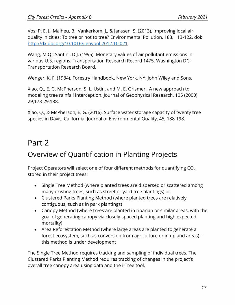
Project Operators will select one of four different methods for quantifying CO2
stored in their project trees:
• Single Tree Method (where planted trees are dispersed or scattered among
many existing trees, such as street or yard tree plantings) or
• Clustered Parks Planting Method (where planted trees are relatively
contiguous, such as in park plantings)
• Canopy Method (where trees are planted in riparian or similar areas, with the
goal of generating canopy via closely-spaced planting and high expected
mortality)
• Area Reforestation Method (where large areas are planted to generate a
forest ecosystem, such as conversion from agriculture or in upland areas) –
this method is under development
The Single Tree Method requires tracking and sampling of individual trees. The
Clustered Parks Planting Method requires tracking of changes in the project’s
overall tree canopy area using data and the i-Tree tool.

City Forest Credits – Appendix B February 2021
18
The Canopy Method requires our scientists to apply GTR tables to data provided by
the Project Operator on tree or forest type being planted, acres, climate zone, and
other information. This is described in more detail in Attachment A at the end of
this Appendix. Quantification for this Canopy method thus depends on data specific
to each project and application of GTR tables. See Attachment A to this Appendix.
A Project Operator thus selects the appropriate quantification method. He or she
then applies that method at different time periods. The Tools used are the Initial
Credit Quantification Tool, the Management Credit Quantification Tool, and the
Final Quantification Tool.
Thus there are six quantification Tools, three for the Single Tree Method and three
for the Clustered Parks Planting Method. The three Tools for each method are used
near the beginning of a project, in the early years of a project, and at the end of the
project in Year 25.
Single Tree Method:
• Single Tree Initial Credit Quantification
• Single Tree Management Credit Quantification
• Single Tree Final Quantification
Clustered Parks Planting Method:
• Clustered Parks Planting Initial Credit Quantification
• Clustered Parks Planting Credit Quantification
• Clustered Parks Planting Final Quantification
The Tool used depends on the time at which the Project Operator seeks Credits.
The Registry will issue credits on the following tiered schedule per Section 9 of the
Planting Protocol:
• After planting of project trees: 10% of projected total CO2e stored by Year 26,
minus a 20% mortality deduction and a 5% Buffer Pool deduction, subject to
quantification conducted under the Registry’s quantification methodology
and verification by an approved third-party verifier;
• After Year 3: 40% of projected total CO2e stored by Year 26, minus a 5%
Buffer Pool deduction, subject to data collection, sampling, mortality data
based on the sampled data, and quantification conducted under the
Registry’s quantification methodology and verification by an approved third-
party verifier;

City Forest Credits – Appendix B February 2021
19
• After year 5: 30% of projected total CO2e stored by Year 26, a 5% Buffer Pool
deduction, subject to data collection, sampling, mortality data based on the
sampled data, and quantification conducted under the Registry’s
quantification methodology and verification by an approved third-party
verifier;
• At the end of the 25-year Project Duration: all remaining credits issued after
final quantification and verification of carbon stored, minus a 5% Buffer Pool
deduction. Thus, at the end of Year 25, the Project Operator will conduct a
final quantification with data collection, sampling, approval of the
quantification methods by the Registry, and third-party verification. At that
time, the Registry will issue “true-up” credits equaling the difference between
credits already issued (which were based on projected CO2e stored) and
credits earned based on final quantification and verification of CO2e stored;
• 5% of total credits earned and issued will be retained by the Registry for a
Registry-wide Reversal Pool.
The Initial Credit Quantification Tool enables the Project Operator to calculate
projected carbon stored in his or her project using planting data. The Tool applies a
20% mortality deduction as well as a 5% Buffer Pool deduction. The Project
Operator can request to use an alternative value for the 20% mortality reduction.
Justification for the value must be provided to the Registry based on historic
mortality data for projects with similar species, planting stock, site quality and
management regime.
The Management Credit Tool is used for Credits that can be issued in Year 4 and
Year 6. The Management Credit Tool requires planting data, calculation of a sample
number and sample sites, and then sampling of project trees to determine the
presence of trees. This sampling produces a mortality adjustment that allows
estimation of CO2e storage after Years 4 and 6.
The Final Quantification Tool is used at the end of a project, in Year 25. It is the
same basic Tool as the Credit Management Tool used in Years 4 and 6, except that
it also requires measurement of dbh (diameter at breast height).
This Appendix B contains detailed examples of four of the six Tools - Single Tree
Initial Credit Quantification Tool, Single Tree Management Credit Quantification
Tool, Single Tree Final Quantification Tool, and a Clustered Parks Planting Final
Quantification Tool, with associated spreadsheet tables and calculations. The other
Tools are available upon request.

City Forest Credits – Appendix B February 2021
20
Before describing those Tools in detail, here is a summary of the steps used in each
of the three different processes.
Illustrative Summary of Quantification Steps in Four of
the Tools
This section summarizes the steps in three Single Tree Tools used to quantify
carbon storage in tree planting projects. These steps are set out in instructions on
each sheet of the Quantification Spreadsheets. The steps will be much clearer to
many readers when viewed within the spreadsheets rather than read here without
tables, fields, and inputs. The next section of this Appendix – entitled Quantification
Methods and Examples – gives screen shots of the spreadsheets with explanatory
text.
Steps for Single Tree Initial Credit Quantification
1) For each planting site, collect this information
a. Unique site number
b. Unique tree number (may be several tree numbers at same site if
remove & replace)
i. Tree species planted
ii. Date planted
c. Tree number removed
i. Date removed
d. GPS coordinates (lat/long)
e. Notes
2) Photograph tree site or provide imaging of sufficient resolution to discern
individual trees
i. If using photographs, take photos at the four outer corners of
each site, and also at 50 foot intervals on diagonal lines running
between corners
ii. Include time stamp and GPS coordinates
3) The Tool will deduct 20% for mortality and 5% for the program-wide Buffer
Pool and then show projected CO2e storage and Credits
City Forest Credits – Appendix B February 2021
21
a. The Project Operator can request to use an alternative value for the
20% mortality reduction. Justification for the value must be provided to
the Registry based on historic mortality data for projects with similar
species, planting stock, site quality and management regime.
Steps for the Single Tree Management Credit Quantification
1) Collect the planting data described in 1 above, specifically,
a. Unique site number
b. Unique tree number (may be several tree numbers at same site if
remove & replace)
i. Tree species planted
ii. Date planted
c. GPS coordinates (lat/long)
d. Notes
2) Use the Sample Size Calculator that we provide and the Stored CO2 per Tree
Look-Up Table to determine the number of tree sites to sample. We define a
“tree site” as the location where a project tree was planted, and use the term
“site” instead of “tree” because some planted trees may no longer be present
in the sites where they were planted.
3) Randomly sample tree sites collecting data on species, status (alive, dead,
removed, replaced).
4) With this sampled data, the Tool will then calculate projected CO2 storage
and credits, and will set those out for Years 4 and 6, along with quantified Co-
Benefits.
Steps for the Single Tree Final Quantification
1) Collect the planting data described in 1 above, or use the data already
collected, specifically,
a. Unique site number
b. Unique tree number (may be several tree numbers at same site if
remove & replace)
i. Tree species planted
ii. Date planted
c. GPS coordinates (lat/long)

City Forest Credits – Appendix B February 2021
22
d. Notes
2) Use the Sample Size Calculator that we provide and the Stored CO2 per Tree
Look-Up Table to determine the number of tree sites to sample. We define a
“tree site” as the location where a project tree was planted, and use the term
“site” instead of “tree” because some planted trees may no longer be present
in the sites where they were planted.
3) Randomly sample tree sites collecting data on species, status (alive, dead,
removed, replaced), diameter at breast height (dbh) (to nearest inch), and
photo of tree site (may be with or without the tree planted) with geocoded
location and date.
4) Fill in the table provided showing the number of live trees sampled in each 1”
dbh class by tree-type.
5) Combine data from the step 5 table with the CO2 Stored by DBH Look-Up
Table for your climate zone to calculate CO2 stored by sampled trees for each
tree-type.
6) Fill in the table provided showing number of sites planted, sites sampled and
status of sampled tree sites by tree-type. This table calculates Extrapolation
Factors.
7) Combine data from tables in step 7 (Extrapolation Factors) and step 6 to
scale-up CO2 stored from the sample to the population of trees planted.
8) Fill in the table provided to incorporate error estimates of ±15% to CO2
stored by the entire tree population.
9) Fill in the table provided to incorporate estimates of co-benefits.
Steps for the Clustered Parks Planting Final Quantification
Method
1) Describe the project (i.e., dates trees planted, locations and climate zone).
2) Create a planting list that contains data on the numbers of trees planted by
species (with tree-type for each species obtained from the table provided).
3) Fill-in the table provided using data from the Stored CO2 per Unit Canopy
Look-Up Table for 25 years after planting and numbers of trees planted by
tree-type to calculate the Project Index.
4) Use i-Tree Canopy to calculate total project area and area in tree canopy.
5) In the table provided, multiply the area in tree canopy by the Project Index to
calculate total CO2 stored by trees planted in the project area.

City Forest Credits – Appendix B February 2021
23
6) Fill-in the table provided to incorporate error estimates of ±15% to CO2
stored by the entire tree population.
7) Fill-in the table provided to incorporate estimates of co-benefits.
Quantification Methods and Examples
Data Collection for all Single Tree Quantification and Tools
At planting, Project Operators must collect the data listed below. Project Operators
can update that data as the Project proceeds.
Single Tree Initial Credit Quantification and Tool
The steps above summarized the quantification Tools for four Tools described in
this Appendix. Below is a detailed walk-through of the Single Tree Quantification.
Project operators will use this process and Tools to request Credits in projects
where trees are not planted contiguously.
Example Data Collection Table
date
planted site id# species
tree
id # x coord y coord
live (orig/replace
#1/replace #2)
standing dead
or vacant site image#1 image#2
date
removed date replaced notes
9/15/2016 1 Celtis reticulata 1 33.96872 -117.344
9/15/2016 2 Pistacia chinensis 2 32.96752 -117.263
9/15/2016 3 Platanus racemosa 3 32.87346 -116.84
Date planted
Site Id#, a unique number assigned to each spot a tree is planted at.
Species name (botanical name)
Tree Id#, the unique number that coincides with each tree that was planted at the site. When each tree has just been planted, and there are not
any dead or missing trees, the tree id#s will all be the same as the site#s. As trees get replaced, the list of tree id#s will increase. In the example
below, site# 1 has a replacement tree planted in it, therefore what was originally tree #1 is now tree #4. If tree #4 is the next one at the project
latitude and longitude or x and y coordinates of where each tree is located. These data are used to accurately locate the site for remeasurement.
Data Collection Date: 04/24/2018 Crew: Julie and Ed
Directions
Create a data sheet with the same fields seen in the example below.
At the time of data collection soon after planting, record the following information:
Date of data collection.
Names of the crew that collected that data.
At the time of data collection soon after planting record the following information on each tree:

City Forest Credits – Appendix B February 2021
24
The Registry will provide the Tools that contains look-up tables and calculations
built into the spreadsheet so that projects can enter their project data and then
walk through the sheets to quantify CO2 and co-benefits.

City Forest Credits – Appendix B February 2021
25
Overview
Single Tree Projects Initial Credit Quantification Tool for the Southern California Coast Climate Zone
Steps
2) If the anticipted mortality rate in 25 years is NOT the default 20% of planted sites, the value is entered into row 6 on the Credits sheet. Justification for the
value must be provided to the Registry based on historic mortality data for projects with similar species, planting stock, site quality and management regime.
3) Initial Credits will be automatically calculated and presented in Tables 3 and 4 (column H), incorporating anticipated tree losses and the 5% buffer pool
deduction.
The analyst can use this method to calculate the amount of CO2 (in metric tonnes, t) estimated to be stored by live project trees after 25 years. Credits
based on the estimated CO2 storage can be issued at three points in time – 10% within one year after planting, 40% after year 3, and 30% after year 5,
minus 5% that will go into a program-wide buffer pool to insure against catastrophic loss of trees. At the end of the project, in year 25, Operators will receive
credits for all CO2 stored, minus credits already issued.
Project Operators will follow the Steps listed below to obtain an initial estimate that assumes 20% mortality. Basic tree planting data on all trees planted
needs to be collected at the time of planting. Users will submit this spreadsheet to the Registry with other documentation so that the verifier can verify the
planting before initial credits are issued. Sampled data will be used to obtain credits at subsequent points in time.
6) Table 7 automatically provides estimates of co-benefits for live trees after 25 years in Resource Units (e.g., kWh) per year and $ per year.
1) Compile data on the numbers of trees planted by species to fill in the Planting List (Table 1). When planting project trees collect the following data on each
planted tree: species, site id#, tree id# and location (latitude and longitude). We use the term “site” instead of “tree” because some planted trees may no longer
be present in the sites where they were planted.
5) For planning purposes only, users can enter a low and high price of CO2 ($ per t) in Table 5. Table 6 incorporates error estimates of ±15% to calculate low and
high amounts of CO2 stored.

City Forest Credits – Appendix B February 2021
26
Planting List
Enter the species and number planted as shown in Table 1 below.
Directions
Table 1. Planting List Table 2. Summary of Planting Sites
ScientificName CommonName
Tree-Type
Abbreviation
No. Sites
Planted Tree-Type Tree-Type Abbreviation No. Sites Planted
Acacia baileyana Bailey acacia BES Brdlf Decid Large (>50 ft) BDL 140
Acacia decurrens green acacia BEM Brdlf Decid Med (30-50 ft) BDM 94
Acacia longifolia Sydney golden wattle BES Brdlf Decid Small (<30 ft) BDS 16
Acacia melanoxylon black acacia BEL Brdlf Evgrn Large (>50 ft) BEL 0
Acer palmatum Japanese maple BDS Brdlf Evgrn Med (30-50 ft) BEM 0
Acer rubrum red maple BDL Brdlf Evgrn Small (<30 ft) BES 0
Acer saccharinum silver maple BDL Conif Evgrn Large (>50 ft) CEL 0
Acer species maple BDL Conif Evgrn Med (30-50 ft) CEM 0
Agonis flexuosa peppermint tree; Australian willow myrtle BES Conif Evgrn Small (<30 ft) CES 0
Albizia julibrissin mimosa BDS 16 Total Sites Planted 250
Alnus cordata Italian alder BDM
Alnus rhombifolia white alder BDL
Annona cherimola cherimoya BES
Araucaria bidwillii bunya bunya CEL
Araucaria columnaris coral reef araucaria CEL
Araucaria heterophylla Norfolk Island pine CEL
Arbutus unedo strawberry tree BES
Archontophoenix cunninghamianking palm PES
Arecastrum romanzoffianum queen palm PES
Bauhinia variegata mountain ebony BDS
Betula pendula European white birch BDM
Betula species birch BDM 94
Brachychiton populneus kurrajong BEM
Brahea armata Mexican blue palm PES
Brahea edulis Guadalupe palm PES
Brahea species brahea palm PES
Broadleaf Deciduous Large broadleaf deciduous large BDL 140
Broadleaf Deciduous Medium broadleaf deciduous medium BDM
Broadleaf Deciduous Small broadleaf deciduous small BDS
Broadleaf Evergreen Large broadleaf evergreen large BEL
Broadleaf Evergreen Medium broadleaf evergreen medium BEM
Broadleaf Evergreen Small broadleaf evergreen small BES
Broussonetia papyrifera paper mulberry BDM
Butia capitata jelly palm PES
Calliandra tweedii Trinidad flame bush BES
Callistemon citrinus lemon bottlebrush BES
Callistemon viminalis weeping bottlebrush BES
Calocedrus decurrens incense cedar CEL
1) In Table 1 record the number of sites planted for each tree species.
2) If species are not listed, add them to the bottom of Table 1.

City Forest Credits – Appendix B February 2021
27
Initial Credits
This sheet calculates the Credits that can be issued in Year 1. It uses a default
mortality of 20%. Project Operators may adjust that mortality deduction if they
demonstrate to the Registry justification based on historic mortality data for
projects with similar species, planting stock, site quality and management regime.
Credits issued in Years 4 and 6 will depend on mortality based on sampling of trees
in those years.
Directions
Mortality Deduction (%): 20%
10% 40% 30%
No. Sites
Planted
No. Live
Trees
Mortality
Deduction
(%)
25-yr CO2 stored
(kg/tree)
Tot. 25-yr CO2 stored
w/ losses and 5%
deduction (t)
Initial
CO2 (t)
4 Years
CO2 (t)
6 Years
CO2 (t)
BDL 140 112 0.20 1,794.13 190.9 19.09 76.36 57.27
BDM 94 75 0.20 629.52 45.0 4.50 17.99 13.49
BDS 16 13 0.20 422.19 5.1 0.51 2.05 1.54
BEL 0 0 0.20 0.00 0.0 0.00 0.00 0.00
BEM 0 0 0.20 0.00 0.0 0.00 0.00 0.00
BES 0 0 0.20 0.00 0.0 0.00 0.00 0.00
CEL 0 0 0.20 0.00 0.0 0.00 0.00 0.00
CEM 0 0 0.20 0.00 0.0 0.00 0.00 0.00
CES 0 0 0.20 0.00 0.0 0.00 0.00 0.00
250 200 2,845.8 241.0 24.10 96.40 72.30
Table 3. Credits are based on 10%, 40% and 30% at Years 1, 4 and 6 after planting, respectively, of the projected CO2
stored by live trees 25-years after planting. These values account for anticipated tree losses and the 5% buffer pool
deduction.
Enter the default 20% anticipted mortality rate (% of planted sites without trees in 25 years) into cell D6. Using the
information you provide and background data, the tool calculates the amount of Credits that could be issued at years 1
(10%), 4 (40%) and 6 (30%) after planting. The mortality deductions (% loss) is applied to account for anticipated tree
losses. A 5% buffer pool deduction is applied that will go into a program-wide pool to insure against catastrophic loss of
trees.

City Forest Credits – Appendix B February 2021
28
Total CO2
Table 4. Grand Total CO2 Stored after 25 years (all live trees, includes tree losses and buffer pool deduction)
Tree-Type
No. Sites
Planted
Mortality
Deduction
(%)
Total Live
Trees After
Mortality
25-yr CO2
stored
(kg/tree)
CO2 Tot. - No
Deductions
(t)
Grand Total
CO2 w/
Deductions (t)
Brdlf Decid Large (>50 ft) 140 0.20 112 1,794.13 251.2 190.9
Brdlf Decid Med (30-50 ft) 94 0.20 75 629.52 59.2 45.0
Brdlf Decid Small (<30 ft) 16 0.20 13 422.19 6.8 5.1
Brdlf Evgrn Large (>50 ft) 0 0.20 0 0.00 0.0 0.0
Brdlf Evgrn Med (30-50 ft) 0 0.20 0 0.00 0.0 0.0
Brdlf Evgrn Small (<30 ft) 0 0.20 0 0.00 0.0 0.0
Conif Evgrn Large (>50 ft) 0 0.20 0 0.00 0.0 0.0
Conif Evgrn Med (30-50 ft) 0 0.20 0 0.00 0.0 0.0
Conif Evgrn Small (<30 ft) 0 0.20 0 0.00 0.0 0.0
250 200 2,845.8 317.1 241.00
In Table 4 the tool infers the amount of CO2 stored after 25 years based on the anticipated population
of live trees. Values in column H account for anticipated tree losses and the 5% buffer pool deduction.

City Forest Credits – Appendix B February 2021
29
CO2 Summary
Directions
Table 5. CO2 value
CO2 $ per
tonne Tree-Type
Total CO2
(t) at 25
years
Low $
value
High $
value
Low $20.00 Brdlf Decid 241.00 $4,820.04 $9,640.09
High $40.00 Brdlf Evgrn 0.00 $0.00 $0.00
Conif Evgrn 0.00 $0.00 $0.00
Total 241.00 $4,820.04 $9,640.09
CO2 (t) Total $ Total $
Grand Total CO2
(t) at 25 years: 241.00 $4,820.04 $9,640.09
High Est. with
Error: 277.15 $5,543.05 $11,086.10
Low Est. with
Error: 204.85 $4,097.04 $4,097.04
± 15% error = ± 10% formulaic ± 3% sampling
± 2% measurement
In Table 5, enter the low and high price of CO2 in $ per tonne (t).
Table 6 incorporates error estimates of ±15% to the high and low estimates of the
total CO2 (t) stored by the live tree population after 25 years. For planning
purposes only, it calculates dollar values.
Table 6. Summary of CO2 stored after 25 years (all live
trees, includes tree losses)

City Forest Credits – Appendix B February 2021
30
Co-Benefits
Table 10. Co-Benefits per year after 25 years (all live trees, includes tree losses)
Ecosystem Services
Res Units
Totals Res Unit/site Total $ $/site
Rain Interception (m3/yr) 734.20 2.94 $1,512.86 $6.051
CO2 Avoided (t, $20/t/yr) 16.86 0.07 $337.17 $1.349
Air Quality (t/yr)
O3 0.0998 0.0004 $1,100.35 $4.401
NOx 0.0244 0.0001 $686.65 $2.747
PM10 0.0517 0.0002 $1,072.53 $4.290
Net VOCs 0.0010 0.0000 $10.34 $0.041
Air Quality Total 0.1768 0.0007 $2,869.86 $11.48
Energy (kWh/yr & kBtu/yr)
Cooling - Elec. 39,554.23 158.22 $4,612.02 $18.45
Heating - Nat. Gas 18,835.65 75.34 $234.40 $0.94
Energy Total ($/yr) $4,846.42 $19.39
Grand Total ($/yr) $9,566.31 $38.27
Using the information you provide and background data, the tool provides
estimates of co-benefits after 25 years in Resource Units per year and $ per year.

City Forest Credits – Appendix B February 2021
31
Single Tree Management Credit Quantification and Tool
Overview
Follow these directions, and also update the Data Collection Sheet that you
completed at time of planting. See page 10 above.
Steps
8) Table 7 automatically infers the amount of CO2 stored after 25 years from the sample to the population of live trees.
9) For planning purposes only, users can enter a low and high price of CO2 ($ per t) in Table 8. Table 9 incorporates error estimates of ±15% to calculate low and
high amounts of CO2 stored.
10) Table 10 automatically provides estimates of co-benefits for live trees after 25 years in Resource Units (e.g., kWh) per year and $ per year.
6) Enter data on the number of live trees and vacant sites from the Data Collection table into Table 5 on the Sample Data sheet.
7) Credits will be automatically calculated in Table 6.
2) Compile data on the numbers of trees planted by species from the Data Collection table and use this information to fill in the Planting List (Table 1).
3) The Sample Size Calculator will automatically determine the number of sites to sample (Table 3).
The analyst can use this method to calculate the amount of CO2 (in metric tonnes, t) estimated to be stored by live project trees for Years 4 and 6 crediting.
These credits are based on sample data that revise the estimated CO2 storage 25 years after planting from the anticipated value that assumed 20%
mortality. Credits are issued at the rates of 40% in Year 4, and 30% in Year 6, minus 5% that will go into a program-wide buffer pool to insure against
catastrophic loss of trees. This tool calculates benefits assuming trees are 25-years old with average dbh's of 20", 16" and 10" for large, medium and small
tree-types, respectively.
To summarize the Tool briefly, Project Operators will sample trees from a random selection within the project area. They will record if each sample tree is
alive, dead or missing. They will also photo-sample each sampling site and submit the images geocoded & time stamped. This tool then calculates CO2
stored, co-benefits, and the number of Credits that may be issued at Years 4 and 6. Users will submit this spreadsheet to the Registry with photo images so
that the Registry can verify the process and sampled data. It is important to note that co-benefits to human health, satisfaction, attendance/absenteeism,
and quality of life are not quantified by this tool, but can be compelling reasons for partners to invest in local projects.
5) Collect data at each sample site using the Data Collection table included in this workbook. For further instructions see the Data Collection sheet.
4) Create a random sample of sites to visit. For further instructions see the Random Sampling sheet. Note that if you choose to collect data at more than one of
the allowed time steps (immediately after planting, after year 3, and after year 5), DIFFERENT random samples must be drawn at each of those times to avoid any
sampling bias.
1) Plant project trees and collect the following data on each planted tree using the data collection table included in this workbook: species, site id#, tree id# and
location (latitude and longitude). We use the term “site” instead of “tree” because some planted trees may no longer be present in the sites where they were
planted.
Single Tree Project Management Credit Quantification Tool for the Tropical Climate Zone

City Forest Credits – Appendix B February 2021
32
Planting List
Single Tree Projects Initial Credit Quantification Tool for the Southern California Coast Climate Zone
Steps
2) If the anticipted mortality rate in 25 years is NOT the default 20% of planted sites, the value is entered into row 6 on the Credits sheet. Justification for the
value must be provided to the Registry based on historic mortality data for projects with similar species, planting stock, site quality and management regime.
3) Initial Credits will be automatically calculated and presented in Tables 3 and 4 (column H), incorporating anticipated tree losses and the 5% buffer pool
deduction.
The analyst can use this method to calculate the amount of CO2 (in metric tonnes, t) estimated to be stored by live project trees after 25 years. Credits
based on the estimated CO2 storage can be issued at three points in time – 10% within one year after planting, 40% after year 3, and 30% after year 5,
minus 5% that will go into a program-wide buffer pool to insure against catastrophic loss of trees. At the end of the project, in year 25, Operators will receive
credits for all CO2 stored, minus credits already issued.
Project Operators will follow the Steps listed below to obtain an initial estimate that assumes 20% mortality. Basic tree planting data on all trees planted
needs to be collected at the time of planting. Users will submit this spreadsheet to the Registry with other documentation so that the verifier can verify the
planting before initial credits are issued. Sampled data will be used to obtain credits at subsequent points in time.
6) Table 7 automatically provides estimates of co-benefits for live trees after 25 years in Resource Units (e.g., kWh) per year and $ per year.
1) Compile data on the numbers of trees planted by species to fill in the Planting List (Table 1). When planting project trees collect the following data on each
planted tree: species, site id#, tree id# and location (latitude and longitude). We use the term “site” instead of “tree” because some planted trees may no longer
be present in the sites where they were planted.
5) For planning purposes only, users can enter a low and high price of CO2 ($ per t) in Table 5. Table 6 incorporates error estimates of ±15% to calculate low and
high amounts of CO2 stored.
Directions
Table 1. Planting List Table 2. Summary of Planting Sites
ScientificName CommonName
Tree-Type
Abbreviation
No. Sites
Planted Tree-Type Tree-Type Abbreviation No. Sites Planted
Acacia baileyana Bailey acacia BES Brdlf Decid Large (>50 ft) BDL 140
Acacia decurrens green acacia BEM Brdlf Decid Med (30-50 ft) BDM 94
Acacia longifolia Sydney golden wattle BES Brdlf Decid Small (<30 ft) BDS 16
Acacia melanoxylon black acacia BEL Brdlf Evgrn Large (>50 ft) BEL 0
Acer palmatum Japanese maple BDS Brdlf Evgrn Med (30-50 ft) BEM 0
Acer rubrum red maple BDL Brdlf Evgrn Small (<30 ft) BES 0
Acer saccharinum silver maple BDL Conif Evgrn Large (>50 ft) CEL 0
Acer species maple BDL Conif Evgrn Med (30-50 ft) CEM 0
Agonis flexuosa peppermint tree; Australian willow myrtle BES Conif Evgrn Small (<30 ft) CES 0
Albizia julibrissin mimosa BDS 16 Total Sites Planted 250
Alnus cordata Italian alder BDM
Alnus rhombifolia white alder BDL
Annona cherimola cherimoya BES
Araucaria bidwillii bunya bunya CEL
Araucaria columnaris coral reef araucaria CEL
Araucaria heterophylla Norfolk Island pine CEL
Arbutus unedo strawberry tree BES
Archontophoenix cunninghamianking palm PES
Arecastrum romanzoffianum queen palm PES
Bauhinia variegata mountain ebony BDS
Betula pendula European white birch BDM
Betula species birch BDM 94
Brachychiton populneus kurrajong BEM
Brahea armata Mexican blue palm PES
Brahea edulis Guadalupe palm PES
Brahea species brahea palm PES
Broadleaf Deciduous Large broadleaf deciduous large BDL 140
Broadleaf Deciduous Medium broadleaf deciduous medium BDM
Broadleaf Deciduous Small broadleaf deciduous small BDS
Broadleaf Evergreen Large broadleaf evergreen large BEL
Broadleaf Evergreen Medium broadleaf evergreen medium BEM
Broadleaf Evergreen Small broadleaf evergreen small BES
Broussonetia papyrifera paper mulberry BDM
Butia capitata jelly palm PES
Calliandra tweedii Trinidad flame bush BES
Callistemon citrinus lemon bottlebrush BES
Callistemon viminalis weeping bottlebrush BES
Calocedrus decurrens incense cedar CEL
1) In Table 1 record the number of sites planted for each tree species.
2) If species are not listed, add them to the bottom of Table 1.

City Forest Credits – Appendix B February 2021
33
Data Collection – Calculating your Sample Size
Data Collection – Identifying your Random Sample of Planting Sites
Table 3. Sample Size Calculator
Description Value
1) Margin of Error (15% required) 15%
2) Confidence level (95% required) 95%
3) Total number of project sites 250 Directions
4) Mean stored CO2 per tree (kg) 1189
5) Standard deviation of stored CO2 (kg) 978
6) Expected proportion of tree survival (75% required) 75%
Calculated sample size 115
Age BDL BDM BDS BEL BEM BES CEL CEM CES Avg. Std. Dev.
5 380 66 45 103 58 102 13 30 47
10 1,282 249 152 354 185 281 203 127 167
15 2,444 550 338 724 376 453 964 317 315
20 3,638 957 610 1,175 615 588 2,021 621 475
25 4,719 1,450 976 1,673 883 695 2,021 1,059 640 1,189 978
30 5,627 2,009 1,442 2,191 1,162 812 2,021 1,647 807
35 6,364 2,610 2,013 2,711 1,434 992 2,021 2,402 974
40 6,977 3,231 2,695 3,222 1,684 1,316 2,021 3,337 974
Table 4. Stored CO2 (kg) by tree type for years after planting in the Tropical climate zone.
Use the Sample Size Calculator that we provide to determine the number of sites to sample. We
use the term “site” instead of “tree” because some planted trees may no longer be present in the
sites where they were planted.
1) Margin of error, the default value of 15% is used.
2) Confidence level, the default value of 95% is used.
3) The total number of original sites is automatically filled in from the Planting List tab.
4) Mean stored CO2 for all tree types 25 years after planting is automatically filled in from Table 4
below.
5) Standard deviation of the average CO2 stored for all tree types 25 years after planting is
automatically filled in from the Table 4.
6) Expected proportion of tree survival – for sampling purposes we conservatively estimate that
75% of the planted trees are expected to survive. This value is used as the default in the Sample
Size Calculator.
Directions
Use this tool to create a random list of site IDs to sample.
No. Sites
to Sample
Random List
of Site IDs
1 69
2 97
3 134
4 200
5 170
6 116
7 133
8 236
9 195
10 104
11 21
12 139
13 215
14 186
1) In Column A create a numbered row for each of the sites to be sampled (110) in example.
2) In cell B6, replace the XXXX in the following formula with the total number of planted sites, =RANDBETWEEN(1,XXXX).
3) Copy and paste that formula into cell B7. You will get a #NUM! error in that cell. Double click that cell and then press
CTRL+SHIFT+ENTER to enter this as an array formula.
4) Copy cell B7 down for as many rows as you are required to sample, the resulting values should all be unique.
5) Starting in cell B6 you have a list of random site numbers where you will collect data.
6) Note that DIFFERENT random samples must be drawn each time crediting is sought to avoid any sampling bias.
2) Replace the XXXX in the following formula with the total number of sites,
=LARGE(ROW($1:$XXXX)*NOT(COUNTIF($B$5:B5,ROW($1:$XXXX))),RANDBETWEEN(1,(XXXX+2-1)-ROW(B5)))

City Forest Credits – Appendix B February 2021
34
Data Collection – Field Sample Data Collection Sheet
Sample Data
Example Data Collection Table
date
planted site id# species tree id # x coord y coord
live (orig/replace
#1/replace #2)
standing dead or
vacant site image#1 image#2
date
removed
date
replaced notes
9/15/2016 1 Celtis reticulata 4 33.968715 -117.343649 R#1 1 2 3/1/2017 4/5/2017 Original tree (#1) removed & replaced (#4)
9/15/2016 2 Pistacia chinensis 2 32.967521 -117.263458 vacant 3 4 2/21/2017 Dead tree (#2) removed , not replaced
9/15/2016 3 Platanus racemosa 3 32.873459 -116.839654 Orig 5 6 Originally planted tree (#3) alive
Data Collection Date: 08/11/2018 Crew: Julie and Ed
If the tree is alive, record if it is the original one planted (original) or a replacement (replace#1, replace#2).
Record if the tree is dead (standing) or missing (vacant site).
To request Credits, consult the Sample Size Calculator to determine the required number of random samples.
During subsequent field sampling sessions you may find it helpful to take a copy of your original data sheets along for reference when attempting to locate each
tree.
Date removed, the date when the tree was removed.
Date replaced, the date when the replacement tree was planted.
Notes, information concerning tree status, health, etc.
Use the Random Sampling Tool to create a random list of site IDs to sample.
image#1, the unique number for the first image of this site.
image#2, the unique number for the second image of this site taken at 90 degrees to the first.
Directions
Create a data sheet with the same fields seen in the example below.
Dirtections
2) In Table 5 Cols. H-I enter the number of vacant sites sampled (original tree not replaced, 1st replacement removed and not replaced, 2nd replacement removed and not replaced) by tree type.
Table 5. Sample Data on Tree Numbers
Sample Data
Number of
Sites
Originially
Planted
Sampled -
No. Live
Original
Planting
Sampled -
No. Live 1st
Replacemen
ts
Sampled -
No. Live 2nd
Replacemen
ts
Total Sites
Sampled -
Live Trees
Sampled Dead -
Original
Planting Not
Replaced
Sampled -
Dead - 1st
Replacements,
Not Replaced
Sampled -
Dead - 2nd
Replacements,
Not Replaced
Total Sites
Sampled -
Vacant /
Dead Trees
Total
Sites
Sampled
Original
Planting
Survival
(%)
Current
Survival w/
Replacements
(%)
Extrap-
olation
Factor
Total Number
Live Trees
Inferred from
Sample
Brdlf Decid Large (>50 ft) 140 39 4 1 44 12 1 0 13 57 68 77 2.46 108
Brdlf Decid Med (30-50 ft) 94 26 1 1 28 12 3 0 15 43 60 65 2.19 61
Brdlf Decid Small (<30 ft) 16 6 1 0 7 3 0 0 3 10 60 70 1.60 11
Brdlf Evgrn Large (>50 ft) 0 0 0 0 0 0 0 0
Brdlf Evgrn Med (30-50 ft) 0 0 0 0 0 0 0 0
Brdlf Evgrn Small (<30 ft) 0 0 0 0 0 0 0 0
Conif Evgrn Large (>50 ft) 0 0 0 0 0 0 0 0
Conif Evgrn Med (30-50 ft) 0 0 0 0 0 0 0 0
Conif Evgrn Small (<30 ft) 0 0 0 0 0 0 0 0
250 71 6 2 79 27 4 0 31 110 65 72 180
1) In Table 5 Cols. D-F enter the number of live trees sampled (originally planted, 1st and 2nd replacements) by tree type.

City Forest Credits – Appendix B February 2021
35
Credits at Years 4 and 6 After Planting
Directions
10% 40% 30%
No. Sites
Planted
No. Live
Trees
Mortality
Deduction
(%)
Tot. 25-yr CO2
stored w/
mortality (t)
Tot. 25-yr CO2
stored minus 5%
deduction (t)
Initial CO2
(t)
4 Years CO2
(t)
6 Years CO2
(t)
BDL 140 108 0.23 510.0 484.5 48.45 193.80 145.35
BDM 94 61 0.35 88.8 84.3 8.43 33.73 25.30
BDS 16 11 0.30 10.9 10.4 1.04 4.15 3.11
BEL 0 0 0 0.0 0.0 0.00 0.00 0.00
BEM 0 0 0 0.0 0.0 0.00 0.00 0.00
BES 0 0 0 0.0 0.0 0.00 0.00 0.00
CEL 0 0 0 0.0 0.0 0.00 0.00 0.00
CEM 0 0 0 0.0 0.0 0.00 0.00 0.00
CES 0 0 0 0.0 0.0 0.00 0.00 0.00
250 180 0.28 609.7 579.2 57.92 231.68 173.76
Table 6. Credits are based on 10%, 40% and 30% at Years 1, 4, and 6 after planting, respectively, of the projected CO2 stored
by live trees 25-years after planting. These values account for tree losses based on sampling results and 5% buffer pool
deduction.
Using the information you provide and background data, the tool calculates the amount of Credits that could be issued at
years 1 (10%), 4 (40%) and 6 (30%) after planting. A mortality deduction (% loss) is applied to account for tree losses based
on sampling results.

City Forest Credits – Appendix B February 2021
36
Total CO2
Table 7. Grand Total CO2 Stored after 25 years (all live trees, includes tree losses)
Tree-Type
No. Sites
Planted
Extrap.
Factor
Total Live
(Original +
Replaced
Trees)
Sampled
Total
Number Live
Trees
Inferred
from Sample
Sample CO2
Stored (kg)
End of Year 25
(w/ mortality)
CO2 (t) Stored
at the End of
Year 25 Minus
5% Buffer
Deduction
Brdlf Decid Large (>50 ft) 140 2.46 44 108 207,641.2 484.50
Brdlf Decid Med (30-50 ft) 94 2.19 28 61 40,607.5 84.33
Brdlf Decid Small (<30 ft) 16 1.60 7 11 6,830.3 10.38
Brdlf Evgrn Large (>50 ft) 0 0 0 0 0.00 0.00
Brdlf Evgrn Med (30-50 ft) 0 0 0 0 0.00 0.00
Brdlf Evgrn Small (<30 ft) 0 0 0 0 0.00 0.00
Conif Evgrn Large (>50 ft) 0 0 0 0 0.00 0.00
Conif Evgrn Med (30-50 ft) 0 0 0 0 0.00 0.00
Conif Evgrn Small (<30 ft) 0 0 0 0 0.00 0.00
250 79 180 255,079.1 579.21
In Table 7 the tool infers the amount of CO2 stored after 25 years from the sample to the population of live
trees.

City Forest Credits – Appendix B February 2021
37
CO2 Summary
Table 8. CO2 value
CO2 $ per
tonne Tree-Type
Total CO2
(t) at 25
years
Low $
value
High $
value
Low $20.00 Brdlf Decid 579.21 $11,584.20 $23,168.39
High $40.00 Brdlf Evgrn 0.00 $0.00 $0.00
Conif Evgrn 0.00 $0.00 $0.00
Total 579.21 $11,584.20 $23,168.39
CO2 (t) Total $ Total $
Grand Total CO2
(t) at 25 years: 579.21 $11,584.20 $23,168.39
High Est. with
Error: 666.09 $13,321.82 $26,643.65
Low Est. with
Error: 492.33 $9,846.57 $9,846.57
± 15% error = ± 10% formulaic ± 3% sampling
± 2% measurement
Table 9. Summary of CO2 stored after 25 years (all live
trees, includes tree losses)

City Forest Credits – Appendix B February 2021
38
Co-Benefits
Single Tree Final Credit Quantification and Tool
Overview
Project Operators will use and update their Data Collection sheet created at
planting. See page 10 above. The Tool described below will guide them through
final quantification at Year 26.
The P.O. calculates the amount of CO2 stored by live project trees 26 years after
initial planting, based on sampling of the resource. The following steps are required
and illustrated for a hypothetical planting of 250 street/front yard sites in
Sacramento, with 95 trees sampled 26-years after planting.
Table 7. Co-Benefits per year after 25 years (all live trees, includes tree losses)
Ecosystem Services
(Resource Units)
Resource
Units (Totals)
Resource
Unit/site Total $ $/site
Rain Interception (m3/yr) 1,038.93 4.16 $502.26 $2.009
CO2 Avoided (t, $20/t/yr) 10.46 0.04 $209.18 $0.837
Air Quality (t/yr)
O3 0.0819 0.0003 $2,966.76 $11.867
NOx 0.0367 0.0001 $1,330.25 $5.321
PM10 0.0465 0.0002 $5,258.16 $21.033
Net VOCs -0.1759 -0.0007 -$1,295.22 -$5.181
Air Quality Total -0.0109 0.0000 $8,259.96 $33.04
Energy (kWh/yr & kBtu/yr)
Cooling - Elec. 23,486.42 93.95 $3,823.82 $15.30
Heating - Nat. Gas 14,510.13 58.04 $188.82 $0.76
Energy Total ($/yr) $4,012.64 $16.05
Grand Total ($/yr) $12,984.04 $51.94
Using the information you provide and background data, the tool provides
estimates of co-benefits after 25 years in Resource Units per year and $ per year.

City Forest Credits – Appendix B February 2021
39
Planting List
Steps
7) In the CO2 Summary sheet, Table 16, enter the low and high price of CO2 in $ per tonne (t).
5) Visit and collect data at each site. For further instructions see the data collection sheet.
6) Enter the number of live trees sampled in each 1” dbh class by tree-type in the tables 5-7 on the Sampled Data sheet. Then enter the number of dead
and not replaced (vacant) and dead that were replaced in tables 10-12.
This tool is used to support a request for final credits 26 years after planting when most trees have matured. The approach calculates the amount of CO2 stored
by live project trees in metric tonnes (t) on a tree-by-tree basis, based on sampling of a full inventory of the resource.
1) Create a planting list that contains data on the numbers of trees planted by species. Other information to record includes tree location and date
planted.
2) Use the information gathered in step one to fill-in the Planting List (Table 1) by recording the number of sites planted for each tree species. We use
the term “site” instead of “tree” because some planted trees may no longer be present in the sites where they were planted.
3) Use the Sample Size Calculator (Table 3) to determine the number of sites to sample. See directions on the sheet for more information.
4) Create a random sample of sites to visit and collect data at each site. See the Random Sample sheet for more information. Use a DIFFERENT random
sample each time credits are sought.
Directions
Table 1. Planting List Table 2. Summary of Planting Sites
ScientificName CommonName
Tree-Type
Abbreviation
No. Sites
Planted Tree-Type Tree-Type Abbreviation No. Sites Planted
Acacia baileyana Bailey acacia BES Brdlf Decid Large (>50 ft) BDL 140
Acacia decurrens green acacia BEM Brdlf Decid Med (30-50 ft) BDM 94
Acacia longifolia Sydney golden wattle BES Brdlf Decid Small (<30 ft) BDS 16
Acacia melanoxylon black acacia BEL Brdlf Evgrn Large (>50 ft) BEL 0
Acer palmatum Japanese maple BDS Brdlf Evgrn Med (30-50 ft) BEM 0
Acer rubrum red maple BDL Brdlf Evgrn Small (<30 ft) BES 0
Acer saccharinum silver maple BDL Conif Evgrn Large (>50 ft) CEL 0
Acer species maple BDL Conif Evgrn Med (30-50 ft) CEM 0
Agonis flexuosa peppermint tree; Australian willow myrtle BES Conif Evgrn Small (<30 ft) CES 0
Albizia julibrissin mimosa BDS 16 Total Sites Planted 250
Alnus cordata Italian alder BDM
Alnus rhombifolia white alder BDL
Annona cherimola cherimoya BES
Araucaria bidwillii bunya bunya CEL
Araucaria columnaris coral reef araucaria CEL
Araucaria heterophylla Norfolk Island pine CEL
Arbutus unedo strawberry tree BES
Archontophoenix cunninghamianking palm PES
Arecastrum romanzoffianum queen palm PES
Bauhinia variegata mountain ebony BDS
Betula pendula European white birch BDM
Betula species birch BDM 94
Brachychiton populneus kurrajong BEM
Brahea armata Mexican blue palm PES
Brahea edulis Guadalupe palm PES
Brahea species brahea palm PES
Broadleaf Deciduous Large broadleaf deciduous large BDL 140
Broadleaf Deciduous Medium broadleaf deciduous medium BDM
Broadleaf Deciduous Small broadleaf deciduous small BDS
Broadleaf Evergreen Large broadleaf evergreen large BEL
Broadleaf Evergreen Medium broadleaf evergreen medium BEM
Broadleaf Evergreen Small broadleaf evergreen small BES
Broussonetia papyrifera paper mulberry BDM
Butia capitata jelly palm PES
Calliandra tweedii Trinidad flame bush BES
Callistemon citrinus lemon bottlebrush BES
Callistemon viminalis weeping bottlebrush BES
Calocedrus decurrens incense cedar CEL
1) In Table 1 record the number of sites planted for each tree species.
2) If species are not listed, add them to the bottom of Table 1.

City Forest Credits – Appendix B February 2021
40
Data Collection - Sample Size
Data Collection – Calculating a Random Sample of Planting Sites
Table 3. Sample Size Calculator
Description Value
1) Margin of Error (15% required) 15%
2) Confidence level (95% required) 95%
3) Total number of project sites 250 Directions
4) Mean stored CO2 per tree (kg) 1128
5) Standard deviation of stored CO2 (kg) 642
6) Enter: Expected proportion of tree survival 70%
Calculated sample size 95
Use the Sample Size Calculator that we provide to determine the number of sites to sample.
We use the term “site” instead of “tree” because some planted trees may no longer be
present in the sites where they were planted.
3) The total number of original sites is automatically filled in from the Planting List tab.
4) Mean stored CO2 for all tree types 25 years after planting is automatically filled in from Table 4
below.
3) Standard deviation of the average CO2 stored for all tree types 25 years after planting is
automatically filled in from the Table 4.
5) Expected proportion of tree survival – estimates of survival rates can be based on project
experience or pre-sampling. Enter the proportion (%) of expected tree survival into the Sample
Size Calculator (this can be calculated by dividing the expected or known number of trees that
have survived by the total number of trees that were planted, input this number into Cell D9,
which will multipy your value by 100 and display it as a percentage). Note: if you do not have an
estimate for tree survival, 75 should be entered.
1) Margin of error, the default value of 15% is used.
2) Confidence level, the default value of 95% is used.
No. Sites
to
Sample
Random List
of Sites
1 129
2 48
3 64
4 148
5 188
6 201
7 97
8 26
9 65
10 233
11 205
12 167
13 95
2) Replace the XXXX in the following formula with the total number of sites,
=LARGE(ROW($1:$XXXX)*NOT(COUNTIF($B$5:B5,ROW($1:$XXXX))),RANDBETWEEN(1,(XXXX+2-1)-ROW(B5)))
Use this to create a random list of site IDs to sample.
6) Note that DIFFERENT random samples must be drawn each time crediting is sought to avoid any sampling bias.
3) Copy and paste that formula into cell B6. You will get a #NUM! error in that cell. Double click that cell and then press
CTRL+SHIFT+ENTER to enter this as an array formula.
5) Starting in cell B5 you have a list of random site numbers where you will collect data.
Random Sampling Steps
1) Replace the XXXX in the following formula with the total number of sites, =RANDBETWEEN(1,XXXX). Enter this formula in cell B5.
4) Copy cell B6 down for the amount of rows that is equivilant to the amount of sites you are required to sample, the resulting
values should all be unique.
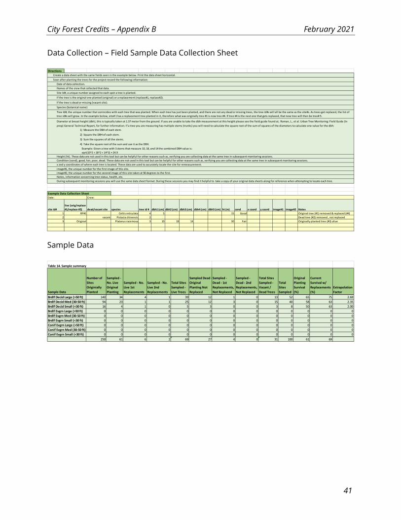
City Forest Credits – Appendix B February 2021
41
Data Collection – Field Sample Data Collection Sheet
Sample Data
Directions
site id#
live (orig/replace
#1/replace #2) dead/vacant site species tree id # dbh1 (cm) dbh2 (cm) dbh3 (cm) dbh4 (cm) dbh5 (cm) ht (m) cond x coord y coord image#1 image#2 Notes
1 RP#1 Celtis reticulata 4 5 15 Good Original tree (#1) removed & replaced (#4)
2 vacant Pistacia chinensis 2 Dead tree (#2) removed , not replaced
3 Original Platanus racemosa 3 10 18 14 30 Fair Originally planted tree (#3) alive
Date: Crew:
image#2, the unique number for the second image of this site taken at 90 degrees to the first.
Notes, information concerning tree status, health, etc.
3) Sum the squares of all the stems.
4) Take the square root of the sum and use it as the DBH.
Example: Given a tree with 3 stems that measure 10, 18, and 14 the combined DBH value is:
sqrt(10^2 + 18^2 + 14^2) = 24.9
Height (ht). These data are not used in this tool but can be helpful for other reasons such as, verifying you are collecting data at the same tree in subsequent monitoring sessions.
image#1, the unique number for the first image of this site.
Condition (cond), good, fair, poor, dead. These data are not used in this tool but can be helpful for other reasons such as, verifying you are collecting data at the same tree in subsequent monitoring sessions.
x and y coordinates of where each tree is located. These data are used to accurately locate the site for remeasurement.
During subsequent monitoring sessions you will use the same data sheet format. During these sessions you may find it helpful to take a copy of your original data sheets along for reference when attempting to locate each tree.
Example Data Collection Sheet
2) Square the DBH of each stem.
Create a data sheet with the same fields seen in the example below. Print the data sheet horizontal.
Soon after planting the trees for the project record the following information:
Date of data collection.
Names of the crew that collected that data.
Site Id#, a unique number assigned to each spot a tree is planted.
If the tree is the original one planted (original) or a replacement (replace#1, replace#2).
If the tree is dead or missing (vacant site).
Species (botanical name)
Tree Id#, the unique number that conincides with each tree that was planted. When each tree has just been planted, and there are not any dead or missing trees, the tree id#s will all be the same as the site#s. As trees get replaced, the list of
tree id#s will grow. In the example below, site# 1 has a replacement tree planted in it, therefore what was originally tree #1 is now tree #4. If tree #4 is the next one that gets replaced, that new tree will then be tree# 5.
Diameter at breast height (dbh), this is typically taken at 1.37 meter from the ground. If you are unable to take the dbh measurement at this height please see the field guide found at, Roman, L., et al. Urban Tree Monitoring: Field Guide (In
prep) General Technical Report, for further information. If a tree you are measuring has multiple stems (trunks) you will need to calculate the square root of the sum of squares of the diameters to calculate one value for the dbh:
1) Measure the DBH of each stem.
Table 14. Sample summary
Sample Data
Number of
Sites
Originially
Planted
Sampled -
No. Live
Original
Planting
Sampled - No.
Live 1st
Replacements
Sampled - No.
Live 2nd
Replacements
Total Sites
Sampled -
Live Trees
Sampled Dead -
Original
Planting Not
Replaced
Sampled -
Dead - 1st
Replacements,
Not Replaced
Sampled -
Dead - 2nd
Replacements,
Not Replaced
Total Sites
Sampled -
Vacant /
Dead Trees
Total
Sites
Sampled
Original
Planting
Survival
(%)
Current
Survival w/
Replacements
(%)
Extrapolation
Factor
Brdlf Decid Large (>50 ft) 140 34 4 1 39 12 1 0 13 52 65 75 2.69
Brdlf Decid Med (30-50 ft) 94 23 1 1 25 12 3 0 15 40 58 63 2.35
Brdlf Decid Small (<30 ft) 16 4 1 0 5 3 0 0 3 8 50 63 2.00
Brdlf Evgrn Large (>50 ft) 0 0 0 0 0 0 0 0 0 0 0 0 0
Brdlf Evgrn Med (30-50 ft) 0 0 0 0 0 0 0 0 0 0 0 0 0
Brdlf Evgrn Small (<30 ft) 0 0 0 0 0 0 0 0 0 0 0 0 0
Conif Evgrn Large (>50 ft) 0 0 0 0 0 0 0 0 0 0 0 0 0
Conif Evgrn Med (30-50 ft) 0 0 0 0 0 0 0 0 0 0 0 0 0
Conif Evgrn Small (<30 ft) 0 0 0 0 0 0 0 0 0 0 0 0 0
250 61 6 2 69 27 4 0 31 100 61 69

City Forest Credits – Appendix B February 2021
42
Total CO2 - Final Credits at 26 Years After Planting
Table 15. Grand Total CO2 Stored (all live trees, includes tree losses)
Tree-Type
No. Sites
Planted
Extrap.
Factor
Total Live
(Original +
Replaced
Trees)
Sampled
Total Number
Live Trees
Inferred from
Sample
Sample
CO2 Tot.
(kg)
Grand
Total CO2
(t)
Brdlf Decid Large (>50 ft) 140 2.69 39 105 54,858.89 147.70
Brdlf Decid Med (30-50 ft) 94 2.35 25 59 23,048.57 54.16
Brdlf Decid Small (<30 ft) 16 2.00 5 10 813.48 1.63
Brdlf Evgrn Large (>50 ft) 0 0 0 0 0.00 0.00
Brdlf Evgrn Med (30-50 ft) 0 0 0 0 0.00 0.00
Brdlf Evgrn Small (<30 ft) 0 0 0 0 0.00 0.00
Conif Evgrn Large (>50 ft) 0 0 0 0 0.00 0.00
Conif Evgrn Med (30-50 ft) 0 0 0 0 0.00 0.00
Conif Evgrn Small (<30 ft) 0 0 0 0 0.00 0.00
250 69 174 78,720.94 203.49
In Table 15 the tool infers the amount of CO2 stored from the sample to the population of live
trees.

City Forest Credits – Appendix B February 2021
43
CO2 Summary
You can enter a price per tonne to see dollar values of Credits.
Table 16. CO2 value Table 17. Summary of CO2 stored
CO2 $ per tonne Tree-Type
Total CO2 (t)
at 25 years Low $ value High $ value
Low $20.00 Brdlf Decid 203.49 $4,069.76 $8,139.52
High $40.00 Brdlf Evgrn 0.00 $0.00 $0.00
Conif Evgrn 0.00 $0.00 $0.00
Total 203.49 $4,069.76 $8,139.52
CO2 (t) Total $ Total $
Grand Total CO2
(t) at 25 years: 203.49 $4,069.76 $8,139.52
High Est. with
Error: 234.01 $4,680.23 $9,360.45
Low Est. with
Error: 172.96 $3,459.30 $3,459.30
± 15% error = ± 10% formulaic ± 3% sampling
± 2% measurement

City Forest Credits – Appendix B February 2021
44
Co-Benefits
Clustered Parks Planting Initial Credit Quantification Method
and Tool
The Registry will provide this Tool and its instructions upon request.
Clustered Parks Planting Management Credit Quantification
Method and Tool
The Registry will provide this Tool and its instructions upon request.
Table 18. Co-Benefits (per year, tree losses included)
Ecosystem Services
Resource
Units (Totals)
Resource
Unit/site Total $ $/site
Rain Interception (m3/yr) 379.18 1.52 $781.31 $3.13
CO2 Avoided (t, $20/t/yr) 9.30 0.04 $186.05 $0.74
Air Quality (t/yr)
O3 0.0514 0.0002 $567.06 $2.27
NOx 0.0126 0.0001 $354.77 $1.42
PM10 0.0268 0.0001 $556.29 $2.23
Net VOCs 0.0005 0.0000 $5.65 $0.02
Air Quality Total 0.0914 0.0004 $1,483.78 $5.94
Energy (kWh/yr & kBtu/yr)
Cooling - Elec. 21,825.56 87.30 $2,544.86 $10.18
Heating - Nat. Gas 7,565.78 30.26 $94.15 $0.38
Energy Total ($/yr) $2,639.01 $10.56
Grand Total ($/yr) $5,090.14 $20.36
Using the information you provide and background data, the tool provides
estimates of co-benefits in Resource Units per year and $ per year. Values
include tree losses based on sampling results.

City Forest Credits – Appendix B February 2021
45
Clustered Parks Planting Final Quantification Method
The PO calculates the amount of CO2 currently stored by planted project trees in
metric tonnes (t) based on the amount of tree canopy (TC) determined from remote
sensing and an index (CO2 per unit canopy area) that is weighted by the mix of
species planted. The following steps are illustrated for a hypothetical planting of
500 tree sites along a creek in Sacramento, CA measured 25-years after planting.
Step 1. Describe the project, quantify the project area, acquire the
following information: numbers of trees planted, date planted, species name and
tree-type for each species, GPS locations and climate zone (Table 1).
The 500 trees were planted 25-years ago along the Bannon Creek Parkway
bordered by Azevedo Dr. (west), Bannon Creek Elementary School (north and east)
and West El Camino Ave. (south) (Figure 1). The Project Area, shown outlined in red
using a Google image in the i-Tree Canopy application, covers 12.5 acres (5.1 ha).
The numbers of trees originally planted are shown by species and tree-type in
Table 1.

City Forest Credits – Appendix B February 2021
46
Figure 1. The Project Area where 500 trees were planted 25-years ago in
Sacramento, CA.

City Forest Credits – Appendix B February 2021
47
Table 1. Planting list for trees planted 25-years ago in the Bannon Creek Parkway
Project Area, Sacramento, CA (Inland Valley climate zone)
Step 2. For each tree-type, locate the Stored CO2 by Age and Unit
Canopy Look-Up Table (Table 2) for the Inland Valley climate zone at, in this case,
25-years after planting. Copy these values into the Project Index Table (Table 3).
Table 2. The Stored CO2 by Age and Unit Canopy Look-Up Table contains values for
each tree-type in the Inland Valley climate zone at 5-year intervals after planting.
Values reflect a single tree's CO2 per unit tree canopy (TC, kg/m2) at selected years
after planting (from McPherson et al. 2016). Values in the highlighted column for
25-year old trees are used in this example.
er TC (kg/m2) BDL BDM BDS BEL BEM BES CEL CEM CES
Age ZESE PYCA PRCE CICA MAGR ILOP SESE PIBR2 PICO5
5 2.4 14.3 5.7 4.9 2.6 4.4 6.6 1.2 5.8
10 5.3 17.5 8.6 8.0 5.2 12.0 17.5 5.5 9.4
15 8.0 19.1 11.7 11.0 7.8 19.6 28.6 13.6 12.1
20 10.7 20.3 14.8 14.0 10.3 26.7 40.0 23.5 14.4
25 13.5 21.1 18.0 16.9 12.8 33.1 52.1 24.9 16.4
30 16.2 21.7 21.2 19.8 15.2 38.8 65.0 25.9 18.3
35 18.9 22.3 24.4 22.6 17.5 44.0 79.2 27.0 20.1
40 21.7 22.7 27.6 25.2 19.8 48.8 95.0 28.1 20.1

City Forest Credits – Appendix B February 2021
48
Step 3. The numbers of trees planted are multiplied by their respective
per tree Stored CO2 index to calculate Project Indices for each tree-type (last
column Table 3). These values are summed (10,766 kg) and divided by the total
number of trees planted (500) to derive the Stored CO2 Project Index (21.53 kg/m2).
This value is the average amount of CO2 stored per unit of tree canopy (TC), after
weighting to account for the mix of species planted.
Table 3. This Project Index Table shows 25-year Project CO2 indices that are
calculated in the fourth column as the products of tree numbers planted (col. 2)
and the per tree values for 25-Yr Stored CO2 (col. 3) from Table 2.
Step 4. Use i-Tree Canopy or another tool to classify tree cover and
estimate the tree canopy (TC) area for the planted tree sites. If using point
sampling, continue adding points until the standard error of the estimate is less
than 5%.
Using i-Tree Canopy, 110 points were randomly located in the Project Area (PA) and
classified as Tree or Non-Tree. The result was 44.9% tree canopy (TC) and 55.1%
non-tree cover, both at ± 4.81% standard error (Std. Er., Table 4). By clicking on the
gear icon next to the upper right portion of the image and selecting ”Report By
Area” the user can prompt i-Tree Canopy to provide an estimate of the area in Tree
or Non-Tree cover. In this example, the PA is 12.5 acres.
Tree-Type
Number
Planted
25-Yr Stored CO2
Indices (kg/m2 TC)
Project Indices
(kg/m2 TC)
BDL 120 13.5 1,614.7
BDM 70 21.1 1,475.8
BDS 50 18.0 899.4
BEL 80 16.9 1,355.8
BEM 55 12.8 704.2
BES 30 33.1 992.4
CEL 50 52.1 2,602.5
CEM 45 24.9 1,121.1
CES 0 16.4 0.0
Total: 500 10,766.0
Project Index: 21.53

City Forest Credits – Appendix B February 2021
49
Table 4. Results from the i-Tree Canopy analysis are percentages of tree and non-
tree cover that are converted to area based on the size of the Project Area (PA, 12.5
acres)
Step 5. To estimate the amount of stored CO2 in the project tree canopy
(TC), multiply the Project Index (from Table 3) by the TC area (m2). Divide by 1,000 to
convert from kg to t.
The product of the Project Index (21.53 kg/m2 TC) and TC (22,713 m2) is 489,050 kg
or 489.1 t CO2 (Table 5).
Table 5. This table shows that an estimated 22,713 m2 of tree canopy (TC) stores
489.1 t of CO2.
Step 6. Incorporate error estimates and prices to illustrate range of
amount stored and value (Table 6).
Table 6. This summary table shows that with 15% of the 489.1 t of CO2 stored
added and subtracted to 489.1 t (see Appendix 1) the actual amount of CO2 stored
is likely to range between 415 t and 562 t. The estimated value, assuming prices of
$20 and $40 per tonne, ranges from $8,314 to $22,496.
Tree Cover Non-Tree Cover Total PA Std Er.
Percent (%) 44.9 55.1 100 4.81
Area (ac) 5.6 6.9 12.5
Area (m2) 22,713 27,873 50,585
Amounts
Tree Canopy Area (m2) 22,713
Project Index 21.53
Stored CO2 (kg) 489,050
Stored CO2 (t) 489.1
CO2 (t) 20.00$ 40.00$
Total CO2 (t): 489.1 9,781$ 19,562$
High Est.: 562.4 11,248$ 22,496$
Low Est.: 415.7 8,314$ 16,628$
± 15% error = ± 10% formulaic ± 3% sampling
± 2% measurement (see Appendix 1)
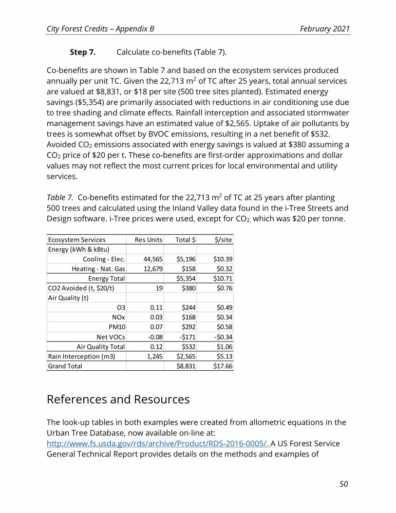
City Forest Credits – Appendix B February 2021
50
Step 7. Calculate co-benefits (Table 7).
Co-benefits are shown in Table 7 and based on the ecosystem services produced
annually per unit TC. Given the 22,713 m2 of TC after 25 years, total annual services
are valued at $8,831, or $18 per site (500 tree sites planted). Estimated energy
savings ($5,354) are primarily associated with reductions in air conditioning use due
to tree shading and climate effects. Rainfall interception and associated stormwater
management savings have an estimated value of $2,565. Uptake of air pollutants by
trees is somewhat offset by BVOC emissions, resulting in a net benefit of $532.
Avoided CO2 emissions associated with energy savings is valued at $380 assuming a
CO2 price of $20 per t. These co-benefits are first-order approximations and dollar
values may not reflect the most current prices for local environmental and utility
services.
Table 7. Co-benefits estimated for the 22,713 m2 of TC at 25 years after planting
500 trees and calculated using the Inland Valley data found in the i-Tree Streets and
Design software. i-Tree prices were used, except for CO2, which was $20 per tonne.
References and Resources
The look-up tables in both examples were created from allometric equations in the
Urban Tree Database, now available on-line at:
http://www.fs.usda.gov/rds/archive/Product/RDS-2016-0005/. A US Forest Service
General Technical Report provides details on the methods and examples of
Ecosystem Services Res Units Total $ $/site
Energy (kWh & kBtu)
Cooling - Elec. 44,565 $5,196 $10.39
Heating - Nat. Gas 12,679 $158 $0.32
Energy Total $5,354 $10.71
CO2 Avoided (t, $20/t) 19 $380 $0.76
Air Quality (t)
O3 0.11 $244 $0.49
NOx 0.03 $168 $0.34
PM10 0.07 $292 $0.58
Net VOCs -0.08 -$171 -$0.34
Air Quality Total 0.12 $532 $1.06
Rain Interception (m3) 1,245 $2,565 $5.13
Grand Total $8,831 $17.66

City Forest Credits – Appendix B February 2021
51
application of the equations and is available online at:
http://www.fs.fed.us/psw/publications/documents/psw_gtr253/psw_gtr253.pdf.
The citations for the archived UTD and the publication are as follows.
McPherson, E. Gregory; van Doorn, Natalie S.; Peper, Paula J. 2016. Urban tree
database. Fort Collins, CO: Forest Service Research Data Archive.
http://dx.doi.org/10.2737/RDS-2016-0005
McPherson, E. Gregory; van Doorn, Natalie S.; Peper, Paula J. 2016. Urban tree
database and allometric equations. General Technical Report PSW-253. U.S.
Department of Agriculture, Forest Service, Pacific Southwest Research Station,
Albany, CA.
http://www.fs.fed.us/psw/publications/documents/psw_gtr253/psw_gtr253.pdf
The i-Tree Canopy Tools is available online at: http://www.itreetools.org/canopy/.
Features of ten software packages for tree inventory and monitoring are evaluated
in this comprehensive report from Azavea: https://www.azavea.com/reports/urban-
tree-monitoring/.
Error Estimates in Carbon Accounting
Our estimates of error include 3 components that are additive and applied to
estimates of total CO2 stored:
Formulaic Error (± 10%) + Sampling Error (± 3%) + Measurement Error (± 2%)
We take this general approach based on data from the literature, recognizing that
the actual error will vary for each project and is extremely difficult to accurately
quantify. We limit the amount of sampling error by providing guidance on the
minimum number of trees to sample in the single-tree approach and the minimum
number of points to sample using i-Tree Canopy. If sample sizes are smaller than
recommended these error percentages may not be valid. Project Operators are
encouraged to provide adequate training to those taking measurements, and to
double-check the accuracy of a subsample of tree dbh measurements and tree
canopy cover classification. A synopsis of the literature and relevant sources are
listed below.

City Forest Credits – Appendix B February 2021
52
Formulaic Error
A study of 17 destructively sampled urban oak trees in Florida reported that the
aboveground biomass averaged 1201 kg. Locally-derived biomass equations
predicted 1208 kg with RMSE of 427 kg. Tree biomass estimates using the UFORE-
ACE (Version 6.5) model splined equations were 14% higher (1368 kg) with an RMSE
that was more than 35% higher than that of the local equation (614 kg or 51%).
Mean total carbon (C) storage in the sampled urban oaks was 423 kg, while i-Tree
ECO over-predicted storage by 14% (483 kg C) with a RMSE of 51% (217 kg C). The
CTCC under-predicted total C storage by 9% and had a RMSE of 611 kg (39%)
Result: Prediction bias for carbon storage ranged from -9% to 14%
Source: Timilsina, N., Staudhammer, C.L., Escobedo, F.J., Lawrence, A. 2014. Tree
biomass, wood waste yield and carbon storage changes in an urban forest.
Landscape and Urban Planning. 127: 18-27.
The study found a maximum 29% difference in plot-level CO2 storage among 4 sets
of biomass equations applied to the same trees in Sacramento, CA. i-Tree Eco
produced the lowest estimate (458 t), Urban General Equations were intermediate
(470 t, and i-Tree Streets was highest (590 t).
Source: Aguaron, E., McPherson, E.G. Comparison of methods for estimating
carbon dioxide storage by Sacramento’s urban forest. pp. 43-71. In Lal, R. and
Augustin, B. (Eds.) Carbon Sequestration in Urban Ecosystems. New York. Springer.
Sampling Error
This error term depends primarily on sample size and variance of CO2 stored per
tree. If sample size is on the order of 80-100 sites for plantings of up to 1,000 trees,
and most of the trees were planted at the same time, so the standard deviation in
CO2 stored is on the order of 30% or less of the mean, then the error is small, about
2-4%.
Source: US Forest Service, PSW Station Statistician Jim Baldwin’s personal
communication and sample size calculator (Sept. 6, 2016)

City Forest Credits – Appendix B February 2021
53
Measurement Error
In this study the mean sampling errors in dbh measurements with a tape were 2.3
mm (volunteers) and 1.4 mm (experts). This error had small effect on biomass
estimates: 1.7% change (from 2.3 mm dbh) in biomass calculated from allometric
equations.
Source: Butt, N., Slade, E., Thompson, J., Malhl, Y., Routta, T. 2013. Quantifying the
sampling error in tree census measurements by volunteers and its effect on carbon
stock estimates. Ecological Applications. 23(4): 936-943.
Attachment A
Approach for Establishing Carbon Dioxide Stored by Tree Canopy in Riparian
Canopy Tree Planting Projects in Austin, TX
This Attachment A provides an example of the Canopy Tree Planting Quantification
Method.
There are two different methods for quantifying carbon dioxide (CO2) storage in
urban forest carbon projects – the Single Tree Method (where planted trees are few
or are scattered among many existing trees) and the Clustered Parks Planting
Method (where planted trees are relatively contiguous). Instead of using the
traditional Clustered Parks Planting Approach for riparian tree planting projects in
Austin, we use a forest ecosystem approach. The traditional approach, which is
based on the biometrics of open-growing urban trees, cannot adequately describe
biomass distribution among closely-spaced trees and the dynamic changes in CO2
stored in dead wood and understory vegetation as a riparian forest stand matures.
In our modified approach the amount of CO2 stored after 25-years by planted
project trees is based on the anticipated amount of tree canopy area (TC). The
forecasted amount of CO2 stored at 25-years is the product of the amount of tree
canopy (TC) and the CO2 Index (CI, t CO2 per acre). This amount is the value from
which the Registry issues credits in the amounts of 10%, 40% and 30% at Years 1, 4
and 6 after planting, respectively. A 5% buffer pool deduction is applied, with these
funds going into a program-wide pool to insure against catastrophic loss of trees. At

City Forest Credits – Appendix B February 2021
54
the end of the project, in year 25, the Operator will receive credits for all CO2
stored, minus credits already issued.
To provide an accurate and complete accounting of carbon pools in these riparian
projects we used the US Forest Service General Technical Report (GTR) NE-343, with
its allometrics for the elm/ash/cottonwood forest ecosystem in the South Central
region (Smith et al., 2006). The table we used (B50) provides carbon stored per
hectare for each of six pools as a function of stand age. We used values for 25-year
old stands for afforestation projects, because the sites contain little carbon in down
dead wood and forest floor material at the time of planting. Data used to derive the
51 forest ecosystem tables came from U.S. Forest Inventory and Assessment plots.
More information on methods used to prepare the tables can be found in Smith et
al. (2006).
Following guidance in GTR NE-343 we adjusted the GTR NE-343 values for live
wood, dead standing and dead down wood using local plot data provided by the
team. According to the plot data the mean amount of C stored in all tree biomass
was 24 t/ha. This value does not include biomass of invasive woody species. Lacking
a measured breakdown of this total for trees among the live, standing dead, and
down dead biomass components, the 24 t/ha was proportionately distributed as
per the GTR (i.e., live: 87%, 20.9 t/ha; standing dead: 7%, 1.7 t/ha; down dead: 6%,
1.4 t/ha). The remaining three carbon pools (understory, forest floor and soil)
remained the same as in GTR Table B50 because their values are independent of
tree biomass. The customized values are shown below in Table 1. Carbon in the
tree pool totals 24 t/ha and accounts for 33% of the total 71.9 t/ha after 25 years for
this forest ecosystem. Soil organic carbon is the single largest pool (56%).
After conversions, the CO2 Index (CI) is 106.7 t CO2 per acre of tree canopy (TC)
and the forecasted amount of CO2 stored after 25-years is the CI x TC. This is
the value from which the Registry will issue credits (Table 1).
Table 1. Estimated amounts of carbon stored in each pool at 25-years after planting
for riparian forest projects in Austin, TX. These values are based on local plot data
for these types of forests and values from GTR NE-343 for the elm/ash/cottonwood
forest ecosystem in the South Central region.

City Forest Credits – Appendix B February 2021
55
Quantification at end of Year 25
• Project provides images of the Project Area from any telemetry, imaging,
remote sensing, i-Tree Canopy, or UAV service, such as Google Earth and
estimate the area in tree canopy cover (acres).
o Projects can use i-Tree Canopy and point sampling to calculate canopy
cover. Using i-Tree Canopy, continue adding points until the standard
error of the estimate for both the tree and non-tree cover is less than
5%. I-Tree Canopy will supply you with the standard errors.
o If tree canopy cover is determined using another approach, such as
image classification, a short description of the approach should be
provided, as well as the QA/QC measures that were used. A tree cover
classification accuracy assessment should be conducted, as with
randomly placed points, and the percentage tree cover classification
accuracy reported.
• Project calculates total CO2 storage at end of Year 25 as follows:
o Multiply the CI (106.73 t CO2/ac TC) times the acres of TC (tree canopy) in
the Project Area.
Data required after Years 3 and 5
• Project provides images of the Project Area from any telemetry, imaging,
remote sensing, or UAV service, such as Google Earth.
• Project uses i-Tree Canopy and point sampling to calculate canopy cover:
elm/ash/cottonwood t/C/ha t/CO2/ha t/CO2/ac % total
live tree 20.9 76.8 31.08 29%
std dead tree 1.7 6.1 2.48 2%
understory 3.3 12.1 4.90 5%
down dead wood 1.4 5.1 2.07 2%
forest floor 4.4 16.1 6.53 6%
soil 40.2 147.4 59.68 56%
total 71.9 263.6 106.73 100%
City Forest Credits – Appendix B February 2021
56
o Using i-Tree Canopy, continue adding points until the standard error of the
estimate for both the tree and non-tree cover is less than 5%. I- Tree Canopy will
supply you with the standard errors.
Progress Requirements for canopy projects after Years 3 and 5:
• After Year 3, projects must show canopy coverage of at least 4% of the
Project Area (average 2.4 foot diameter of canopy per tree of 400 trees per acre)
• After Year 5, projects must show canopy coverage of at least 11% of the
Project Area (average 4 foot diameter of canopy per tress of 400 trees per acre)
Note: if projects exceed these Progress Requirements, they will not receive
credits early or out of schedule. If projects fail to meet the Progress
Requirements, they will not be eligible to request credits until they meet the
Progress Requirements.
References
Smith, James E.; Heath, Linda S.; Skog, Kenneth E.; Birdsey, Richard A. 2006.
Methods for calculating forest ecosystem and harvested carbon with standard
estimates for forest types of the United States. Gen. Tech. Rep. NE-343. Newtown
Square, PA: U.S. Department of Agriculture, Forest Service, Northeastern Research
Station. 216 p.


![V9 series Troubleshooting / Maintenance Manual...V9 Series Reference Manual [1] Explains the functions and operation of the V9 series. 1065NE V9 Series Reference Manual [2] 1066NE](https://img.pdfslide.us/doc/110x75/5fdc0f46901d8161831e54dd/v9-series-troubleshooting-maintenance-v9-series-reference-manual-1-explains.jpg)