APERTURE ANTENNAS - Eefocusdata.eefocus.com/myspace/0/942/bbs/1174163529/a7c74d4.pdf · antenna system for portable equipment—II; ... a principle by which the actual sources on

49. K. Hirasawa and K. Fujimoto, Characteristics of wire anten-nas on a rectangular conducting body, Trans. IEICE J65-B(9):1133–1139 (1982) (in Japanese).

50. K. Fujimoto, A. Henderson, K. Hirasawa, and J. R. James,Small Antennas, Research Studies Press, Chap. 4, 1987, pp.89–110.

51. H. Kuboyama, K. Hirasawa, and K. Fujimoto, UHF-bent-slotantenna system for portable equipment—II; receiving perfor-mance in urban areas, IEEE Trans. Vehic. Technol. VT-36:129–134 (1987).

52. H. Morishita, H. Furuuchi, and K. Fujimoto, Balance-fed L-type loop antenna system for handset, Proc. 1999 Vehicular

Technology Society Int. Conf., 1999, Vol. 3, pp. 1346–1350.

53. Ref. 1, pp. 333–334.

54. Ref. 50, p. 287.

55. K. Fujimoto, Y. Yamada, and K. Tsunekawa, Antenna Systemsfor Mobile Communications, 2nd ed., Denshi Sohgou Publish-ing, Japan, 1999, p. 55 (in Japanese).

56. J. D. Kraus, Antennas 2nd ed., McGraw-Hill, 2002, pp. 293–294.

57. Ref. 47, pp. 59–76.

58. T. Endo, Y. Sunahara, S. Satoh, and T. Katagi, Resonant fre-quency and radiation efficiency of meander line antenna,Trans. IEICE J80 B-II(12):1044–1049 (1997) (in Japanese).

59. L. C. Godara, ed., in Handheld antennas, Handbook of An-

tennas in Wireless Communications, CRC Press, Boca Raton,FL; 2002, Chap. 12, pp. 12-8–12-10.

60. Ref. 47, pp. 120–121.

61. K. Satoh, K. Matsumoto, K. Fujimoto, and K. Hirasawa,Characteristics of a planar inverted-F antenna on a rectan-gular conducting body, Trans. IEICE J71-B(11):1237–1243(1988) (in Japanese).

62. Ref. 1, pp. 440–441.

63. K. Ogawa, High performance technologies for portable radioantennas; toward the harmony of antenna, propagation, hu-man body and systems, J. IEICE 84(11):775–781 (2001).

64. K. Ogawa and T. Uwano, Analysis of a diversity antennacomprising a whip antenna and a planar inverted-F antennafor portable telephones, Trans. IEICE J79-B(12):1008 (1996)(in Japanese).

65. Ref. 1, p. 445; Ref. 55, p. 125.

66. Ref. 1, p. 447.

67. M. Ali, G. J. Hates, H. S. Hwang, and R. A. Sadler, Design ofmultiband internal antenna for third generation mobilephone handsets, IEEE Trans. Anten. Propag. 51(7):1452–1461 (2003).

68. Z. Ying, Design of a branch multi-band antenna and efficiencyenhancement, paper presented at Nordic Antenna Symp.2000, Lund, Sweden, 2000.

69. H. T. Chen, K. L. Wong, and T. W. Chiou, PIFA with a mean-dered and folded patch for the dual-band mobile phone appli-cation, IEEE Trans. Anten. Propag. 51(9):2468–2471 (2003).

70. A. Itakura, Y. Okano, and M. Abe, A study on double reso-nance H-type slot antenna, Trans. IEICE J86-B(12):2533–2542 (2003).

71. H. Morishita and K. Fujimoto, A balance-fed loop antenna sys-tem for handsets, Trans. IEICE E82-A(7):1138–1143 (1999).

72. K. Egawa, T. Oga, and H. Haruki, A development of built-inantenna for W-CDMA visual terminals, 2002 Int. Symp. on

Anten. and Propag. YRP, Japan, pp. 235–238.

73. T.Fukasawa, K. Kopdama,S. Makino, Diversity Antenna for

Portable Telephone with Two Boxes, Tech. Report IEICEAP2002-78, 2002, pp. 87–90.

APERTURE ANTENNAS

DENNIS KOZAKOFF

Devry UniversityAlpharetta, Georgia

1. INTRODUCTION

Aperture antennas are most commonly used at microwaveand the millimeter-wave frequencies. There are a largenumber of antenna types for which the radiated electro-magnetic fields can be considered to emanate from a phys-ical aperture. Antennas that fall into this category includereflector antennas, lenses, and horn antennas. The geom-etry of the aperture may be square, rectangular, circular,elliptical, or virtually any other shape. The term ‘‘apertureantenna’’ usually has more to do with the method used toanalyze the antenna than the actual form of the antenna.For instance, array antennas viewed as a continuous fieldfunction bounded by a conducting screen can be consid-ered to be an aperture antenna. This would encompass so-called planar (flat-plate) waveguide and microstrip arrays.

Aperture antennas are very popular for aerospace ap-plications because they can be flush-mounted onto thespacecraft or aircraft surface. Their aperture opening canbe covered with an electromagnetic (dielectric) windowmaterial that is transparent to the RF energy to protectthe antenna from the environmental conditions [1]. This isknown as a radome, and it is implemented so as not todisturb the aerodynamic profile of the vehicle, which is ofspecial importance to high-speed aircraft or missiles.

In order to evaluate the distant (far-field) radiationpatterns, it is necessary to know the surface currents thatflow on the radiating surfaces of the antenna aperture. Inmany instances, these current distributions may not beknown exactly and only approximate or experimentalmeasurements can provide estimates. A technique basedon the equivalence principle allows one to make reason-able approximations to the electromagnetic fields on, or inthe vicinity of, the physical antenna aperture structure,which can then be used to compute far field antenna ra-diation patterns.

Field equivalence, first introduced by Schelkunoff [2], isa principle by which the actual sources on an antenna ap-erture are replaced by equivalent sources on an externalclosed surface that is physically outside the antenna ap-erture. The fictitious sources are said to be equivalentwithin a region because they produce the same fields with-in that region. Another key concept is Huygens’ principle[3], which states that the equivalent source at each pointon the external surface is a source of a spherical wave. Thesecondary wavefront can be constructed as the envelope ofthese secondary spherical waves [4].

Using these principles, the electrical and/or magneticfields in the equivalent aperture region can be determinedwith these straightforward, but approximate, methods.The fields elsewhere are assumed to be zero. In most ap-plications, the closed surface is selected so that mostof it coincides with the conducting parts of the physicalantenna aperture structure. This is preferred because the

APERTURE ANTENNAS 365

Previous Page

disappearance of the tangential electrical components overthe conducting parts of the surface reduces the physicallimits of integration. The formula to compute the fields ra-diated by the equivalent sources is exact, but it requiresintegration over the closed surface. The degree of accuracydepends on the knowledge of the tangential components ofthe electromagnetic fields over the closed surface.

Aperture techniques are especially useful for parabolicreflector antennas, where the aperture plane can be de-fined immediately in front of the reflector. Parabolic reflec-tors are usually electrically large. More surprisingly,aperture techniques can also be successfully applied tosmall-aperture waveguide horn antennas. However, forvery small horn antennas with an aperture dimension ofless than approximately one wavelength, the assumptionof zero fields outside the aperture fails unless the horn iscompletely surrounded by a planar conducting flange [5].In this section, the mathematical formulas will be devel-oped to analyze the radiation characteristics of apertureantennas. Emphasis will be given to the rectangular andcircular configurations because they are the most commonlyused geometries. Because of mathematical complexities,the results will be restricted to the far-field region.

One of the most useful concepts is the far-field radia-tion pattern that can be obtained as a Fourier transform ofthe field distribution over the equivalent aperture, andvice versa. Fourier transform theory is extremely impor-tant to the analysis and synthesis of aperture antennas.Obtaining analytical solutions for many simple aperturedistributions in order to design aperture antennas is use-ful. More complex aperture distributions, which do notlend themselves to analytical solutions, can be solved nu-merically. The increased capabilities of the personal com-puter (PC) have resulted in its acceptance as aconventional tool for the antenna designers. The Fouriertransform integral is generally well behaved and does notpresent any fundamental computational problems.

Considering the use of the Fourier transform, first con-sider rectangular apertures in which one aperture dimen-sion is large in wavelengths and the other is small interms of wavelengths. This type of aperture is approxi-mated as a line source and is treated with a one-dimen-sional Fourier transform [6]. For many kinds ofrectangular aperture antennas such as horns, the aper-ture distributions in the two principal-plane dimensionsare independent. These types of distributions are said tobe separable. The total radiation pattern is the product ofthe pattern functions obtained from the one-dimensionalFourier transforms, which corresponds to the two princi-pal-plane distributions.

If the rectangular aperture distribution cannot be sep-arated, the directivity pattern is found in a similar man-ner to the line-source distribution, except that theaperture field is integrated over two dimensions ratherthan one dimension [7]. This double Fourier transform canalso be applied to circular apertures.

For all aperture distributions, the following observa-tions are made [8]:

1. A uniform amplitude distribution yields the maxi-mum directivity (where nonuniform edge-enhanced

distributions for supergain are considered impracti-cal), but at high sidelobe levels.

2. Tapering the amplitude at the center, from a max-imum to a smaller value at the edges, will reduce thesidelobe levels compared with the uniform illumina-tion, but it results in a larger (mainlobe) beamwidthand less directivity.

3. An inverse-taper distribution (amplitude depressionat the center) results in a smaller (mainlobe) beam-width but increases the sidelobe level and reducesthe directivity when compared with the uniform il-luminated case.

4. Depending on the aperture size in wavelengths andthe phase errors, there is a frequency (or wave-length) for which the gain peaks, falling to smallervalues as the frequency is either raised or lowered.

Finally, we consider aperture efficiencies. The aperture ef-ficiency is defined as the ratio of the effective aperture areato the physical aperture area. The beam efficiency is de-fined as the ratio of the power in the mainlobe to the totalradiated power. The maximum aperture efficiency occursfor a uniform aperture distribution, but maximum beamefficiency occurs for a highly tapered distribution. The ap-erture phase errors are the primary limitation of the ef-ficiency of an antenna.

2. HUYGENS’ PRINCIPLE

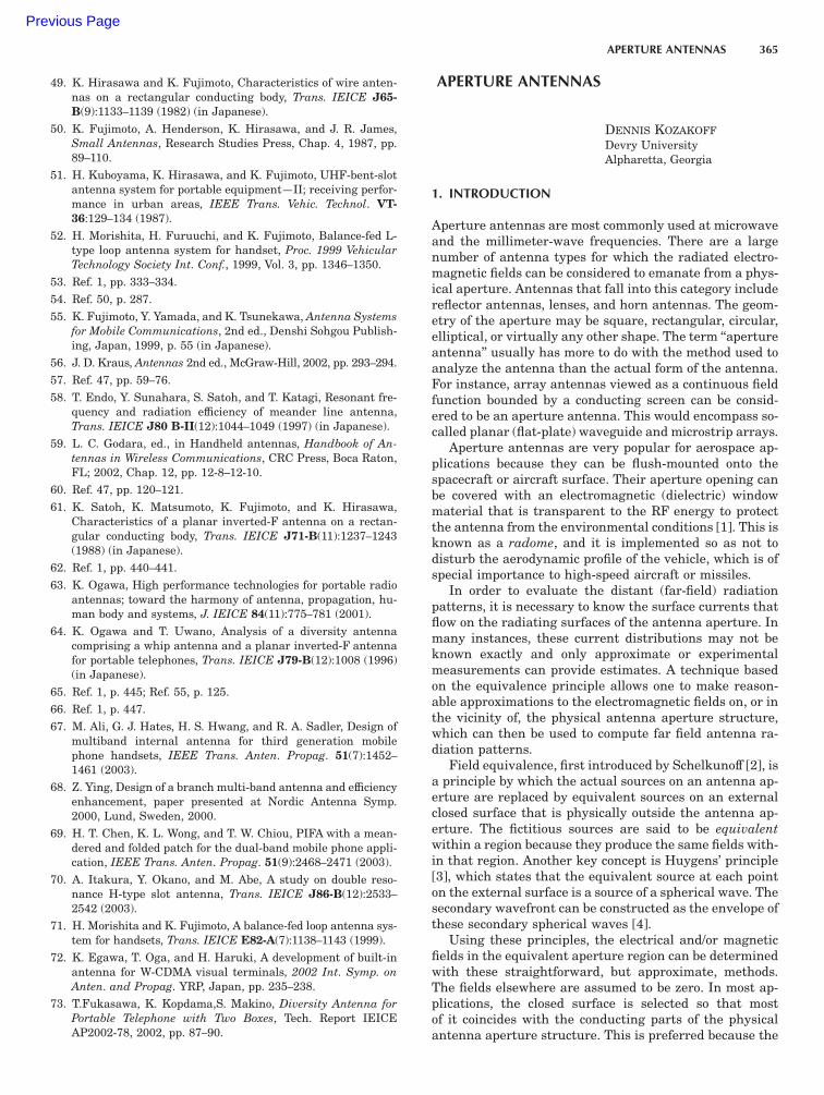
The principle proposed by Christian Huygens (1629–1695)is of fundamental importance to the development of wavetheory [3]. Huygens’ principle states that ‘‘Each point on aprimary wavefront serves as the source of spherical sec-ondary wavelets that advance with a speed and frequencyequal to those of the primary wave. The primary wave-front at some time later is the envelope of all these wave-lets’’ [9]. This is illustrated in Fig. 1 for spherical and

Sphericalwave front

Plane-wave front

(a) (b)

Figure 1. Spherical (a) planar and (b) wavefronts constructedwith Huygens secondary waves.

366 APERTURE ANTENNAS

plane waves modeled as a construction of Huygens’ sec-ondary waves. Actually, the intensities of the secondaryspherical wavelets are not uniform in all directions butvary continuously from a maximum in the direction ofwave propagation to a minimum of zero in the backwarddirection. As a result, there is no backward-propagatingwavefront. The Huygens source approximation is based onthe assumption that the magnetic and electric fields arerelated as a plane wave in the aperture region.

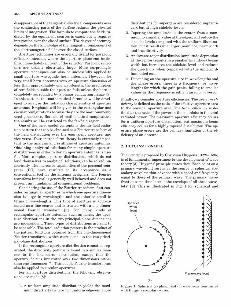
The situation shown in Fig. 2, shows an infinite elec-tromagnetic plane wave incident on an infinite flat sheetthat is opaque to the waves. This sheet has an openingthat is very small in terms of wavelengths. Accordingly,the outgoing wave corresponds to a spherical wavefrontpropagating from a point source. That is, when an incom-ing wave comes against a barrier with a small opening, allexcept one of the effective Huygens point sources areblocked, and the energy coming through the opening be-haves as a single point source. In addition, the outgoingwave emerges in all directions, instead of just passingstraight through the slit.

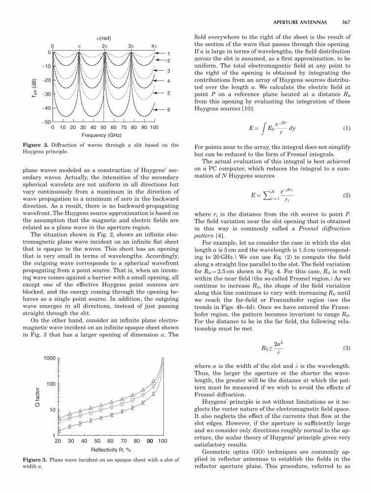
On the other hand, consider an infinite plane electro-magnetic wave incident on an infinite opaque sheet shownin Fig. 3 that has a larger opening of dimension a. The

field everywhere to the right of the sheet is the result ofthe section of the wave that passes through this opening.If a is large in terms of wavelengths, the field distributionacross the slot is assumed, as a first approximation, to beuniform. The total electromagnetic field at any point tothe right of the opening is obtained by integrating thecontributions from an array of Huygens sources distribu-ted over the length a. We calculate the electric field atpoint P on a reference plane located at a distance R0

from this opening by evaluating the integration of theseHuygens sources [10]:

E¼

ZE0

e�jkr

rdy ð1Þ

For points near to the array, the integral does not simplifybut can be reduced to the form of Fresnel integrals.

The actual evaluation of this integral is best achievedon a PC computer, which reduces the integral to a sum-mation of N Huygens sources

E¼XN

i¼1

e�jkri

rið2Þ

where ri is the distance from the ith source to point P.The field variation near the slot opening that is obtainedin this way is commonly called a Fresnel diffractionpattern [4].

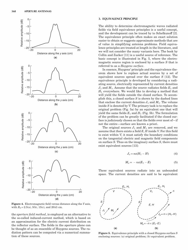
For example, let us consider the case in which the slotlength a is 5 cm and the wavelength is 1.5 cm (correspond-ing to 20 GHz.) We can use Eq. (2) to compute the fieldalong a straight line parallel to the slot. The field variationfor R0¼ 2.5 cm shown in Fig. 4. For this case, R0 is wellwithin the near field (the so-called Fresnel region.) As wecontinue to increase R0, the shape of the field variationalong this line continues to vary with increasing R0 untilwe reach the far-field or Franunhofer region (see thetrends in Figs. 4b–4d). Once we have entered the Fraun-hofer region, the pattern becomes invariant to range R0.For the distance to be in the far field, the following rela-tionship must be met

R0�2a2

lð3Þ

where a is the width of the slot and l is the wavelength.Thus, the larger the aperture or the shorter the wave-length, the greater will be the distance at which the pat-tern must be measured if we wish to avoid the effects ofFresnel diffraction.

Huygens’ principle is not without limitations as it ne-glects the vector nature of the electromagnetic field space.It also neglects the effect of the currents that flow at theslot edges. However, if the aperture is sufficiently largeand we consider only directions roughly normal to the ap-erture, the scalar theory of Huygens’ principle gives verysatisfactory results.

Geometric optics (GO) techniques are commonly ap-plied in reflector antennas to establish the fields in thereflector aperture plane. This procedure, referred to as

0 10 20 30 40 50 60 70 80 90 100

Frequency (GHz)

−50

−40

−30

−20

−10

02

�(rad)

6

5

3

4

1

3

2

0

TF

P (

dB)

4

Figure 2. Diffraction of waves through a slit based on theHuygens principle.

20 30 40 50 60 70 80 90 100

Reflectivity R, %

1

10

100

1000

Q fa

ctor

90

Figure 3. Plane wave incident on an opaque sheet with a slot ofwidth a.


the aperture field method, is employed as an alternative tothe so-called induced-current method, which is based onan approximation for the electric current distribution onthe reflector surface. The fields in the aperture plane canbe thought of as an ensemble of Huygens sources. The ra-diation pattern can be computed via a numerical summa-tion of these sources.

3. EQUIVALENCE PRINCIPLE

The ability to determine electromagnetic waves radiatedfields via field equivalence principles is a useful concept,and the development can be traced by to Schelkunoff [2].The equivalence principle often makes an exact solutioneasier to obtain or suggests approximate methods that areof value in simplifying antenna problems. Field equiva-lence principles are treated at length in the literature, andwe will not consider the many variants here. The book byCollin and Zucker [11] is a useful source of reference. Thebasic concept is illustrated in Fig. 5, where the electro-magnetic source region is enclosed by a surface S that isreferred to as a Huygens surface.

In essence, Huygens’ principle and the equivalence the-orem shows how to replace actual sources by a set ofequivalent sources spread over the surface S [12]. Theequivalence principle is developed by considering a radi-ating source, electrically represented by current densitiesJ1 and M1. Assume that the source radiates fields E1 andH1 everywhere. We would like to develop a method thatwill yield the fields outside the closed surface. To accom-plish this, a closed surface S is shown by the dashed linesthat enclose the current densities J1 and M1. The volumeinside S is denoted by V. The primary task is to replace theoriginal problem (Fig. 5a) by an equivalent one that willyield the same fields E1 and H1 (Fig. 5b). The formulationof the problem can be greatly facilitated if the closed sur-face is judiciously chosen so that the fields over most of—ifnot the entire—surface are known a priori.

The original sources J1 and M1 are removed, and weassume that there exists a field E, H inside V. For this fieldto exist within V, it must satisfy the boundary conditionson the tangential electric and magnetic field componentson surface S. Thus on the imaginary surface S, there mustexist equivalent sources [13]:

Js¼nxðH1 �HÞ ð4Þ

Ms¼ � nxðE1 � EÞ ð5Þ

These equivalent sources radiate into an unboundedspace. The current densities are said to be equivalent

0

−5

−10

−15

−20−20 200

0

−5

−10

−15

−20−20 200

0

−5

−10

−15

−20−20 200

0

−5

−10

−15

−20−20 200

Distance along the y axis (cm)

Rel

ativ

e am

plitu

de (

dB)


Rel

ativ

e am

plitu

de (

dB)


Rel

ativ

e am

plitu

de (

dB)


Rel

ativ

e am

plitu

de (

dB)

(a)

(b)

(c)

(d)

Figure 4. Electromagnetic field versus distance along the Y axis,with R0¼2.5(a), 5(b), 15(c), and 20(d) cm.

J1

V

S

M1

E1, H1 E1, H1

Ms = −n × (E1−E )

Js = n × (H1−H )

V1

S

n

E, H

(a) (b)

Figure 5. Equivalence principle with a closed Huygens surface S

enclosing sources: (a) original problem; (b) equivalent problem.


only outside region V, because they produce the originalfield (E1,H1). A field E or H, different from the original,may result within V.

The sources for electromagnetic fields are always elec-trical currents. However, the electrical current distribu-tion is usually unknown. In certain structures, it may be acomplicated function, particularly for slots, horns, reflec-tors, and lenses. With these types of radiators, the theo-retical work is seldom based on the primary currentdistributions. Rather, the results are obtained with theaid of what is known as aperture theory [14]. This theory isbased on the fact that an electromagnetic field in a source-free, closed region is completely determined by the valuesof tangential E or tangential H fields on the surface of theclosed region. For exterior regions, the boundary conditionat infinity may be employed to close the region. This isexemplified by the following case.

Without changing the E and H fields external to S, theelectromagnetic source region can be replaced by a zero-field region with approximate distributions of electric andmagnetic currents (Js and Ms) on the Huygens surface.This example is overly restrictive and we could specify anyfield within S with a suitable adjustment. However, thezero-internal-field approach is particularly useful whenthe tangential electric fields over a surface enclosing theantenna are known or can be approximated. In this case,the surface currents can be obtained directly from thetangential fields, and the external field can be determined.

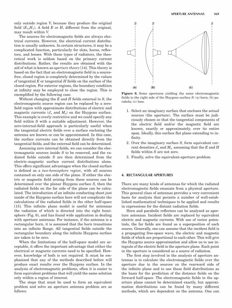
Assuming zero internal fields, we can consider the elec-tromagnetic sources inside S to be removed, and the ra-diated fields outside S are then determined from theelectric–magnetic surface current distributions alone.This offers significant advantages when the closed surfaceis defined as a two-hemisphere region, with all sourcescontained on only one side of the plane. If either the elec-tric or magnetic field arising from these sources can bedetermined over the planar Huygens surface S, then theradiated fields on the far side of the plane can be calcu-lated. The introduction of an infinite conducting sheet justinside of the Huygens surface here will not complicate thecalculations of the radiated fields in the other half-space[15]. This infinite plane model is useful for antennasthe radiation of which is directed into the right hemi-sphere (Fig. 6), and has found wide application in dealingwith aperture antennas. For instance, if the antenna is arectangular horn, it is assumed that the horn transitionsinto an infinite flange. All tangential fields outside therectangular boundary along the infinite Huygens surfaceare taken to be zero.

When the limitations of the half-space model are ac-ceptable, it offers the important advantage that either theelectrical or magnetic currents need to be specified. How-ever, knowledge of both is not required. It must be em-phasized that any of the methods described before willproduce exact results over the Huygens surface. In theanalysis of electromagnetic problems, often it is easier toform equivalent problems that will yield the same solutiononly within a region of interest.

The steps that must be used to form an equivalentproblem and solve an aperture antenna problem are asfollows:

1. Select an imaginary surface that encloses the actualsources (the aperture). The surface must be judi-ciously chosen so that the tangential components ofthe electric field and/or the magnetic field areknown, exactly or approximately, over its entirespan. Ideally, this surface flat plane extending to in-finity.

2. Over the imaginary surface S, form equivalent cur-rent densities Js and Ms, assuming that the E and Hfields within S are not zero.

3. Finally, solve the equivalent-aperture problem.

4. RECTANGULAR APERTURES

There are many kinds of antennas for which the radiatedelectromagnetic fields emanate from a physical aperture.This general class of antennas provides a very convenientbasis for analysis that permits a number of well-estab-lished mathematical techniques to be applied and resultsin expressions for the distant radiation fields.

Horn and parabolic reflectors can be analyzed as aper-ture antennas. Incident fields are replaced by equivalentelectric and magnetic currents. With use of vector poten-tials, the far fields are found as a superposition of eachsource. Generally, one can assume that the incident field isa propagating free-space wave, the electric and magneticfields of which are proportional to each other. This will givethe Huygens source approximation and allow us to use in-tegrals of the electric field in the aperture plane. Each pointin the aperture is considered as a source of radiation.

The first step involved in the analysis of aperture an-tennas is to calculate the electromagnetic fields over theaperture due to the sources on the rearward side ofthe infinite plane and to use these field distributions asthe basis for the prediction of the distance fields on theforward half-space. The electromagnetic fields in the ap-erture plane cannot be determined exactly, but approxi-mation distributions can be found by many differentmethods, which are dependent on the antenna. One can

S S S

(a) (b) (c)

Figure 6. Some apertures yielding the same electromagneticfields to the right side of the Huygens surface S: (a) horn; (b) pa-rabola; (c) lens.


find the far-field radiation pattern for various distribu-tions by, for instance, a Fourier transform relation.

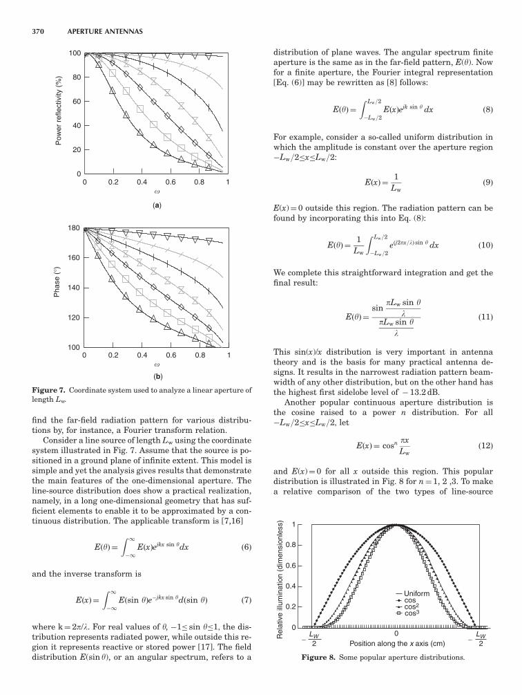
Consider a line source of length Lw using the coordinatesystem illustrated in Fig. 7. Assume that the source is po-sitioned in a ground plane of infinite extent. This model issimple and yet the analysis gives results that demonstratethe main features of the one-dimensional aperture. Theline-source distribution does show a practical realization,namely, in a long one-dimensional geometry that has suf-ficient elements to enable it to be approximated by a con-tinuous distribution. The applicable transform is [7,16]

EðyÞ¼Z 1

�1

EðxÞejkx sin ydx ð6Þ

and the inverse transform is

EðxÞ¼

Z 1

�1

Eðsin yÞe�jkx sin ydðsin yÞ ð7Þ

where k¼ 2p/l. For real values of y, �1� sin y�1; the dis-tribution represents radiated power, while outside this re-gion it represents reactive or stored power [17]. The fielddistribution E(sin y), or an angular spectrum, refers to a

distribution of plane waves. The angular spectrum finiteaperture is the same as in the far-field pattern, E(y). Nowfor a finite aperture, the Fourier integral representation[Eq. (6)] may be rewritten as [8] follows:

EðyÞ¼Z Lw=2

�Lw=2EðxÞejk sin y dx ð8Þ

For example, consider a so-called uniform distribution inwhich the amplitude is constant over the aperture region�Lw=2�x�Lw=2:

EðxÞ¼1

Lwð9Þ

E(x)¼ 0 outside this region. The radiation pattern can befound by incorporating this into Eq. (8):

EðyÞ¼1

Lw

Z Lw=2

�Lw=2eðj2px=lÞ sin y dx ð10Þ

We complete this straightforward integration and get thefinal result:

EðyÞ¼sin

pLw sin yl

pLw sin yl

ð11Þ

This sin(x)/x distribution is very important in antennatheory and is the basis for many practical antenna de-signs. It results in the narrowest radiation pattern beam-width of any other distribution, but on the other hand hasthe highest first sidelobe level of � 13.2 dB.

Another popular continuous aperture distribution isthe cosine raised to a power n distribution. For all�Lw=2�x�Lw=2; let

EðxÞ¼ cosn px

Lwð12Þ

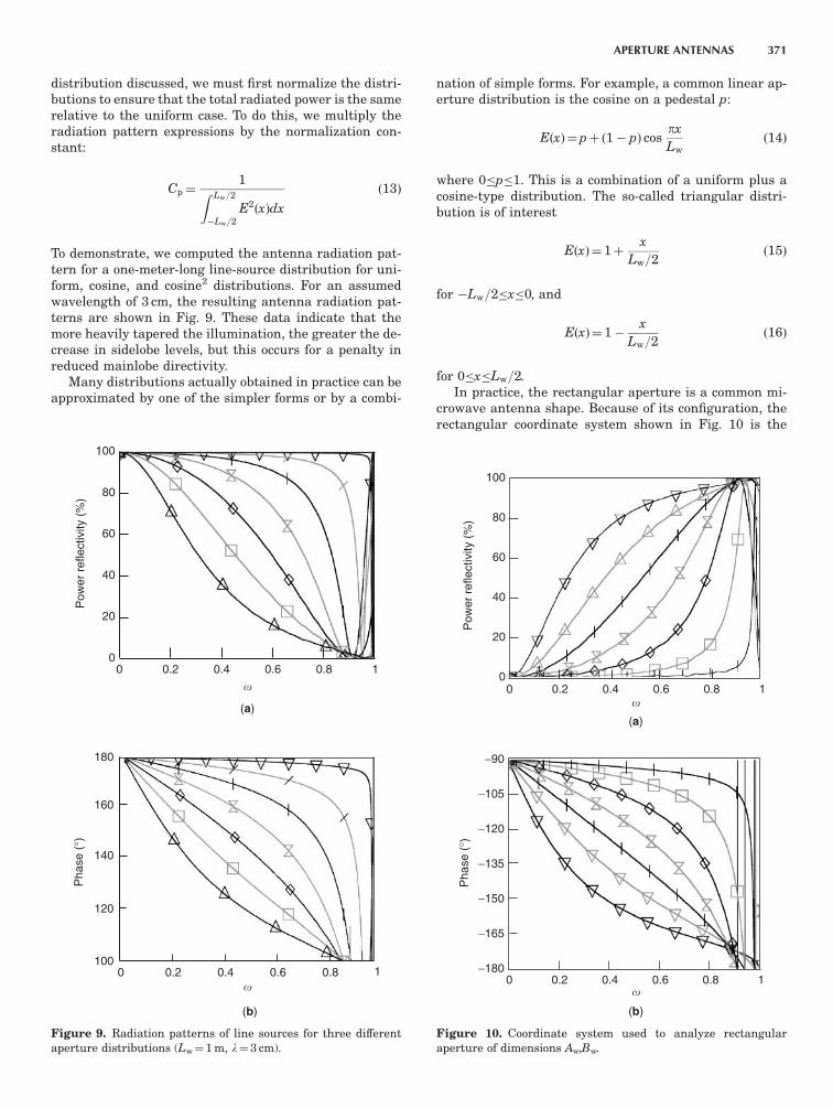
and E(x)¼ 0 for all x outside this region. This populardistribution is illustrated in Fig. 8 for n¼1, 2 ,3. To makea relative comparison of the two types of line-source

0 0.2 0.4 0.6 0.8 10

20

40

60

80

100P

ower

ref

lect

ivity

(%

)

0 0.2 0.4 0.6 0.8 1100

120

140

160

180

Pha

se (

°)

(a)

(b)

Figure 7. Coordinate system used to analyze a linear aperture oflength Lw.

Uniformcoscos2

cos3

LW2− −

LW2Position along the x axis (cm)

Rel

ativ

e ill

umin

atio

n (d

imen

sion

less

)

0

1

0.8

0.6

0.4

0.2

0

Figure 8. Some popular aperture distributions.


distribution discussed, we must first normalize the distri-butions to ensure that the total radiated power is the samerelative to the uniform case. To do this, we multiply theradiation pattern expressions by the normalization con-stant:

Cp¼1

Z Lw=2

�Lw=2E2ðxÞdx

ð13Þ

To demonstrate, we computed the antenna radiation pat-tern for a one-meter-long line-source distribution for uni-form, cosine, and cosine2 distributions. For an assumedwavelength of 3 cm, the resulting antenna radiation pat-terns are shown in Fig. 9. These data indicate that themore heavily tapered the illumination, the greater the de-crease in sidelobe levels, but this occurs for a penalty inreduced mainlobe directivity.

Many distributions actually obtained in practice can beapproximated by one of the simpler forms or by a combi-

nation of simple forms. For example, a common linear ap-erture distribution is the cosine on a pedestal p:

EðxÞ¼pþ ð1� pÞ cospx

Lwð14Þ

where 0�p�1. This is a combination of a uniform plus acosine-type distribution. The so-called triangular distri-bution is of interest

EðxÞ¼ 1þx

Lw=2ð15Þ

for �Lw=2�x�0, and

EðxÞ¼ 1�x

Lw=2ð16Þ

for 0�x�Lw=2.In practice, the rectangular aperture is a common mi-

crowave antenna shape. Because of its configuration, therectangular coordinate system shown in Fig. 10 is the

0 0.2

(a)

0.4 0.6 0.8 10

20

40

60

80

100

Pow

er r

efle

ctiv

ity (

%)

(b)

0 0.2 0.4 0.6 0.8 1100

120

140

160

180

Pha

se (

°)

Figure 9. Radiation patterns of line sources for three differentaperture distributions (Lw¼1 m, l¼3 cm).

0

(a)

(b)

0.2 0.4 0.6 0.8 10

20

40

60

80

100P

ower

ref

lect

ivity

(%

)

0 0.2 0.4 0.6 0.8 1−180

−165

−150

−135

−120

−105

−90

Pha

se (

°)

Figure 10. Coordinate system used to analyze rectangularaperture of dimensions Aw,Bw.


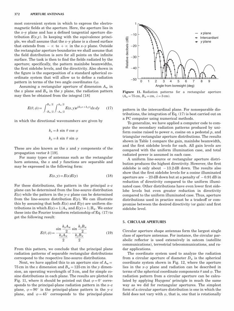
most convenient system in which to express the electro-magnetic fields at the aperture. Here, the aperture lies inthe x–y plane and has a defined tangential aperture dis-tribution E(x,y). In keeping with the equivalence princi-ple, we shall assume that the x–y plane is a closed surfacethat extends from �N to þN in the x–y plane. Outsidethe rectangular aperture boundaries we shall assume thatthe field distribution is zero for all points on the infinitesurface. The task is then to find the fields radiated by theaperture; specifically, the pattern mainlobe beamwidths,the first sidelobe levels, and the directivity. Also shown inthe figure is the superposition of a standard spherical co-ordinate system that will allow us to define a radiationpattern in terms of the two angle coordinates y,j.

Assuming a rectangular aperture of dimension Aw inthe x plane and Bw in the y plane, the radiation patternmay then be obtained from the integral [18]

Eðy;fÞ¼Z Bw=2

�Bw=2

Z Aw=2

�Aw=2Eðx; yÞejðkxxþ kyyÞdx dy ð17Þ

in which the directional wavenumbers are given by

kx¼ k sin y cos j

ky¼ k sin y sin j

These are also known as the x and y components of thepropagation vector k [19].

For many types of antennas such as the rectangularhorn antenna, the x and y functions are separable andmay be expressed in the following form:

Eðx; yÞ¼EðxÞEðyÞ ð18Þ

For these distributions, the pattern in the principal x–zplane can be determined from the line-source distributionEðxÞ while the pattern in the y–z plane can be determinedfrom the line-source distribution EðyÞ. We can illustratethis by assuming that both EðxÞ and EðyÞ are uniform dis-tributions in which EðxÞ¼ 1=Aw and EðyÞ¼ 1=Bw. We enterthese into the Fourier transform relationship of Eq. (17) toget the following result:

Eðy;fÞ¼sin

kxAw

2kxAw

2

sinkyBw

2kyBw

2

ð19Þ

From this pattern, we conclude that the principal planeradiation patterns of separable rectangular distributionscorrespond to the respective line-source distributions.

Next, we have applied this to an aperture size of Aw¼

75 cm in the x dimension and Bw¼ 125 cm in the y dimen-sion, an operating wavelength of 3 cm, and for simple co-sine distributions in each plane. The results are plotted inFig. 11, where it should be pointed out that j¼ 01 corre-sponds to the principal-plane radiation pattern in the x–zplane, j¼ 901 is the principal-plane pattern in the y–zplane, and j¼ 451 corresponds to the principal-plane

pattern in the intercardinal plane. For nonseparable dis-tributions, the integration of Eq. (17) is best carried out ona PC computer using numerical methods.

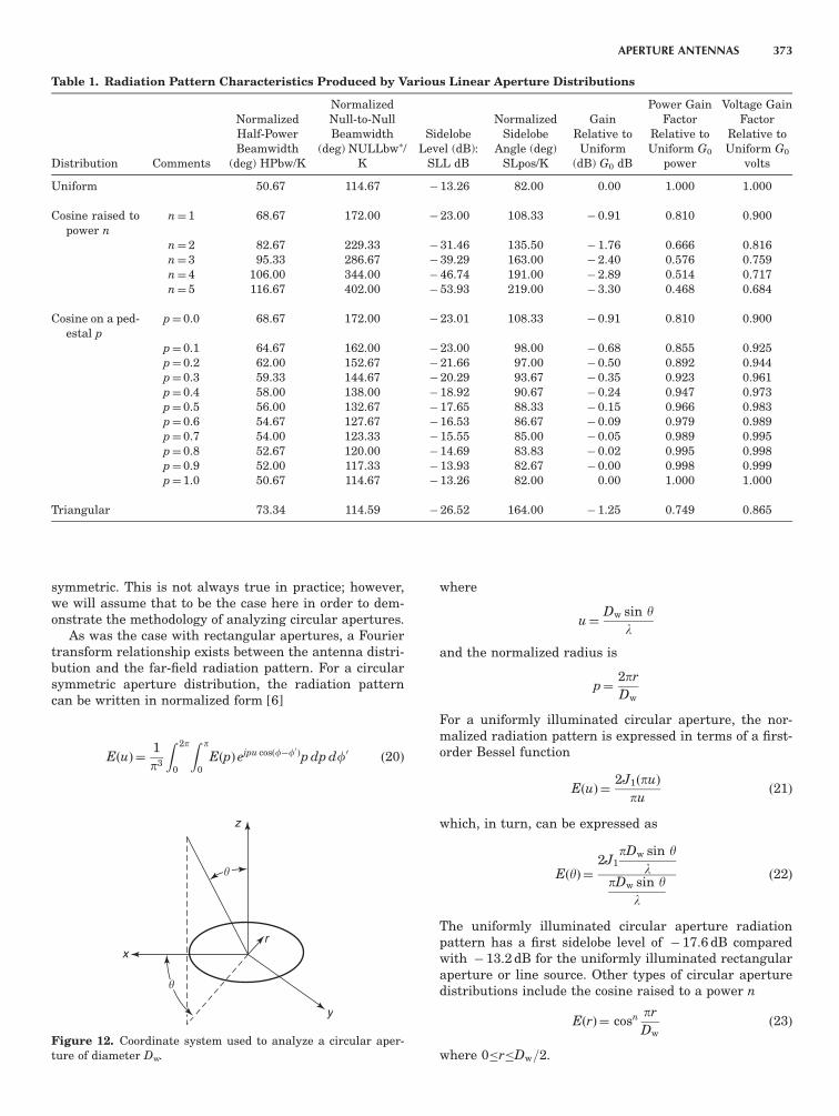
To generalize, we have applied a computer code to com-pute the secondary radiation patterns produced by uni-form cosine raised to power n, cosine on a pedestal p, andtriangular rectangular aperture distributions. The resultsshown in Table 1 compare the gain, mainlobe beamwidth,and the first sidelobe levels for each. All gain levels arecompared with the uniform illumination case, and totalradiated power is assumed in each case.

A uniform line-source or rectangular aperture distri-bution produces the highest directivity. However, the firstsidelobe is only about � 13.2 dB down. The results alsoshow that the first sidelobe levels for a cosine illuminatedaperture are � 23 dB down but at a penalty of � 0.91 dB inreduction of directivity compared to the uniform illumi-nated case. Other distributions have even lower first side-lobe levels but even greater reduction in directivitycompared to the uniform illuminated case. Thus, aperturedistributions used in practice must be a tradeoff or com-promise between the desired directivity (or gain) and firstsidelobe level.

5. CIRCULAR APERTURES

Circular aperture shape antennas form the largest singleclass of aperture antennas. For instance, the circular par-abolic reflector is used extensively in satcom (satellitecommunications), terrestrial telecommunications, and ra-dar applications.

The coordinate system used to analyze the radiationfrom a circular aperture of diameter Dw is the sphericalcoordinate system shown in Fig. 12, where the aperturelies in the x–y plane and radiation can be described interms of the spherical coordinate components y and j. Theradiation pattern from a circular aperture can be calcu-lated by applying Huygens’ principle in much the sameway as we did for rectangular apertures. The simplestform of a circular aperture distribution is one in which thefield does not vary with j, that is, one that is rotationally

x planeIntercardianly plane

−50

1

−10

−20

−30

−40

Angle from boresight (deg)

Rel

ativ

e de

cibe

ls (

dB)

0 1 2 3 4 5 6 7 8 9

Figure 11. Radiation patterns for a rectangular aperture(Aw¼75 cm, Bw¼ cm, l¼3 cm).


symmetric. This is not always true in practice; however,we will assume that to be the case here in order to dem-onstrate the methodology of analyzing circular apertures.

As was the case with rectangular apertures, a Fouriertransform relationship exists between the antenna distri-bution and the far-field radiation pattern. For a circularsymmetric aperture distribution, the radiation patterncan be written in normalized form [6]

EðuÞ¼1

p3

Z 2p

0

Z p

0EðpÞ ejpu cosðf�f0Þp dp df0 ð20Þ

where

u¼Dw sin y

l

and the normalized radius is

p¼2pr

Dw

For a uniformly illuminated circular aperture, the nor-malized radiation pattern is expressed in terms of a first-order Bessel function

EðuÞ¼2J1ðpuÞ

puð21Þ

which, in turn, can be expressed as

EðyÞ¼2J1

pDw sin yl

pDw sin yl

ð22Þ

The uniformly illuminated circular aperture radiationpattern has a first sidelobe level of � 17.6 dB comparedwith � 13.2 dB for the uniformly illuminated rectangularaperture or line source. Other types of circular aperturedistributions include the cosine raised to a power n

EðrÞ¼ cosn pr

Dwð23Þ

where 0�r�Dw=2.

Table 1. Radiation Pattern Characteristics Produced by Various Linear Aperture Distributions

Distribution Comments

NormalizedHalf-PowerBeamwidth

(deg) HPbw/K

NormalizedNull-to-NullBeamwidth

(deg) NULLbw�/K

SidelobeLevel (dB):

SLL dB

NormalizedSidelobe

Angle (deg)SLpos/K

GainRelative toUniform

(dB) G0 dB

Power GainFactor

Relative toUniform G0

power

Voltage GainFactor


volts

Uniform 50.67 114.67 �13.26 82.00 0.00 1.000 1.000

Cosine raised topower n

n¼1 68.67 172.00 �23.00 108.33 �0.91 0.810 0.900

n¼2 82.67 229.33 �31.46 135.50 �1.76 0.666 0.816n¼3 95.33 286.67 �39.29 163.00 �2.40 0.576 0.759n¼4 106.00 344.00 �46.74 191.00 �2.89 0.514 0.717n¼5 116.67 402.00 �53.93 219.00 �3.30 0.468 0.684

Cosine on a ped-estal p

p¼0.0 68.67 172.00 �23.01 108.33 �0.91 0.810 0.900

p¼0.1 64.67 162.00 �23.00 98.00 �0.68 0.855 0.925p¼0.2 62.00 152.67 �21.66 97.00 �0.50 0.892 0.944p¼0.3 59.33 144.67 �20.29 93.67 �0.35 0.923 0.961p¼0.4 58.00 138.00 �18.92 90.67 �0.24 0.947 0.973p¼0.5 56.00 132.67 �17.65 88.33 �0.15 0.966 0.983p¼0.6 54.67 127.67 �16.53 86.67 �0.09 0.979 0.989p¼0.7 54.00 123.33 �15.55 85.00 �0.05 0.989 0.995p¼0.8 52.67 120.00 �14.69 83.83 �0.02 0.995 0.998p¼0.9 52.00 117.33 �13.93 82.67 �0.00 0.998 0.999p¼1.0 50.67 114.67 �13.26 82.00 0.00 1.000 1.000

Triangular 73.34 114.59 �26.52 164.00 �1.25 0.749 0.865

�

�

r

y

x

z

Figure 12. Coordinate system used to analyze a circular aper-ture of diameter Dw.


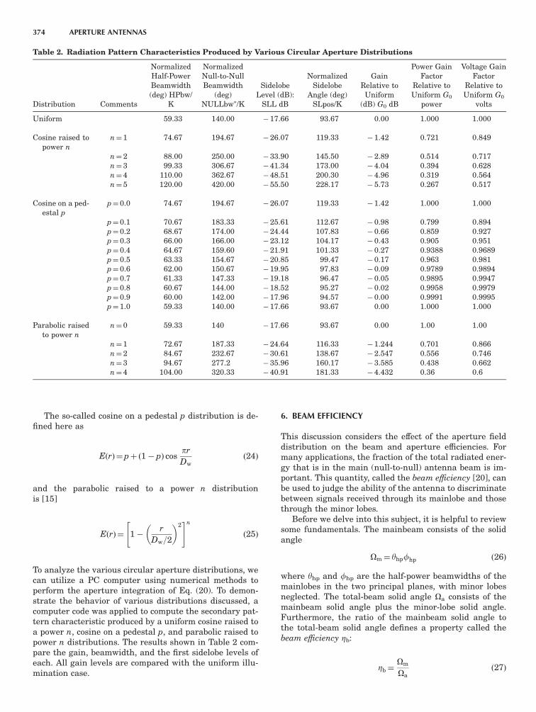
The so-called cosine on a pedestal p distribution is de-fined here as

EðrÞ¼pþ ð1� pÞ cospr

Dwð24Þ

and the parabolic raised to a power n distributionis [15]

EðrÞ¼ 1�r

Dw=2

� �2" #n

ð25Þ

To analyze the various circular aperture distributions, wecan utilize a PC computer using numerical methods toperform the aperture integration of Eq. (20). To demon-strate the behavior of various distributions discussed, acomputer code was applied to compute the secondary pat-tern characteristic produced by a uniform cosine raised toa power n, cosine on a pedestal p, and parabolic raised topower n distributions. The results shown in Table 2 com-pare the gain, beamwidth, and the first sidelobe levels ofeach. All gain levels are compared with the uniform illu-mination case.

6. BEAM EFFICIENCY

This discussion considers the effect of the aperture fielddistribution on the beam and aperture efficiencies. Formany applications, the fraction of the total radiated ener-gy that is in the main (null-to-null) antenna beam is im-portant. This quantity, called the beam efficiency [20], canbe used to judge the ability of the antenna to discriminatebetween signals received through its mainlobe and thosethrough the minor lobes.

Before we delve into this subject, it is helpful to reviewsome fundamentals. The mainbeam consists of the solidangle

Om¼ yhpfhp ð26Þ

where yhp and fhp are the half-power beamwidths of themainlobes in the two principal planes, with minor lobesneglected. The total-beam solid angle Oa consists of themainbeam solid angle plus the minor-lobe solid angle.Furthermore, the ratio of the mainbeam solid angle tothe total-beam solid angle defines a property called thebeam efficiency Zb:

Zb¼Om

Oað27Þ

Table 2. Radiation Pattern Characteristics Produced by Various Circular Aperture Distributions

Distribution Comments

NormalizedHalf-PowerBeamwidth(deg) HPbw/

K

NormalizedNull-to-NullBeamwidth

(deg)NULLbw�/K

SidelobeLevel (dB):

SLL dB

NormalizedSidelobe

Angle (deg)SLpos/K

GainRelative toUniform

(dB) G0 dB

Power GainFactor


power

Voltage GainFactor


volts

Uniform 59.33 140.00 �17.66 93.67 0.00 1.000 1.000

Cosine raised topower n

n¼1 74.67 194.67 �26.07 119.33 �1.42 0.721 0.849

n¼2 88.00 250.00 �33.90 145.50 �2.89 0.514 0.717n¼3 99.33 306.67 �41.34 173.00 �4.04 0.394 0.628n¼4 110.00 362.67 �48.51 200.30 �4.96 0.319 0.564n¼5 120.00 420.00 �55.50 228.17 �5.73 0.267 0.517

Cosine on a ped-estal p

p¼0.0 74.67 194.67 �26.07 119.33 �1.42 1.000 1.000

p¼0.1 70.67 183.33 �25.61 112.67 �0.98 0.799 0.894p¼0.2 68.67 174.00 �24.44 107.83 �0.66 0.859 0.927p¼0.3 66.00 166.00 �23.12 104.17 �0.43 0.905 0.951p¼0.4 64.67 159.60 �21.91 101.33 �0.27 0.9388 0.9689p¼0.5 63.33 154.67 �20.85 99.47 �0.17 0.963 0.981p¼0.6 62.00 150.67 �19.95 97.83 �0.09 0.9789 0.9894p¼0.7 61.33 147.33 �19.18 96.47 �0.05 0.9895 0.9947p¼0.8 60.67 144.00 �18.52 95.27 �0.02 0.9958 0.9979p¼0.9 60.00 142.00 �17.96 94.57 �0.00 0.9991 0.9995p¼1.0 59.33 140.00 �17.66 93.67 0.00 1.000 1.000

Parabolic raisedto power n

n¼0 59.33 140 �17.66 93.67 0.00 1.00 1.00

n¼1 72.67 187.33 �24.64 116.33 �1.244 0.701 0.866n¼2 84.67 232.67 �30.61 138.67 �2.547 0.556 0.746n¼3 94.67 277.2 �35.96 160.17 �3.585 0.438 0.662n¼4 104.00 320.33 �40.91 181.33 �4.432 0.36 0.6


In terms of the radiated intensity E(y,j) of a pencil beamwith boresight at (y¼ 0, j¼0), the beam efficiency can bedefined by [13]

Zb¼

Z yn=2

�yn=2

Z fn=2

�fn=2Eðy;fÞEðy;fÞ� sin ydfdy

Z p

0

Z 2p

0Eðy;fÞEðy;fÞ� sin ydfdy

ð28Þ

where yn and jn are the null-to-null beamwidths in thetwo principal planes. Also, E(y,j)* denotes the conjugate ofE(y,j).

The directivity of the aperture antenna can be ex-pressed as

D¼4pOa¼

4pAp

l2ð29Þ

where Ap is the physical area of the aperture. The apertureefficiency is defined as the ratio of the effective aperturearea Ae to the physical aperture area, or

Za¼Ae

Apð30Þ

so that the ratio of the aperture and beam efficiencies is [8]

Za

Zm

¼AeOa

ApOmð31Þ

where Om is the mainbeam solid angle and Oa is the total-beam solid angle, both of which are measured in steradi-ans (sr). It is important to recognize, then, that the beamefficiency and aperture efficiency are related to each other.

In general, the aperture and beam efficiencies must bemultiplied by a gain degradation factor due to phase er-rors within the aperture given by [21]

Zpe¼ e�ð2pd=lÞ2

ð32Þ

where d is the RMS phase error over the aperture. It isassumed that the correlation intervals of the deviationsare greater than the wavelength. The controlling effect oftapers on the beam and aperture efficiencies tends to de-crease them as the phase error increases. The efficienciesare also reduced by the presence of other phase errors.

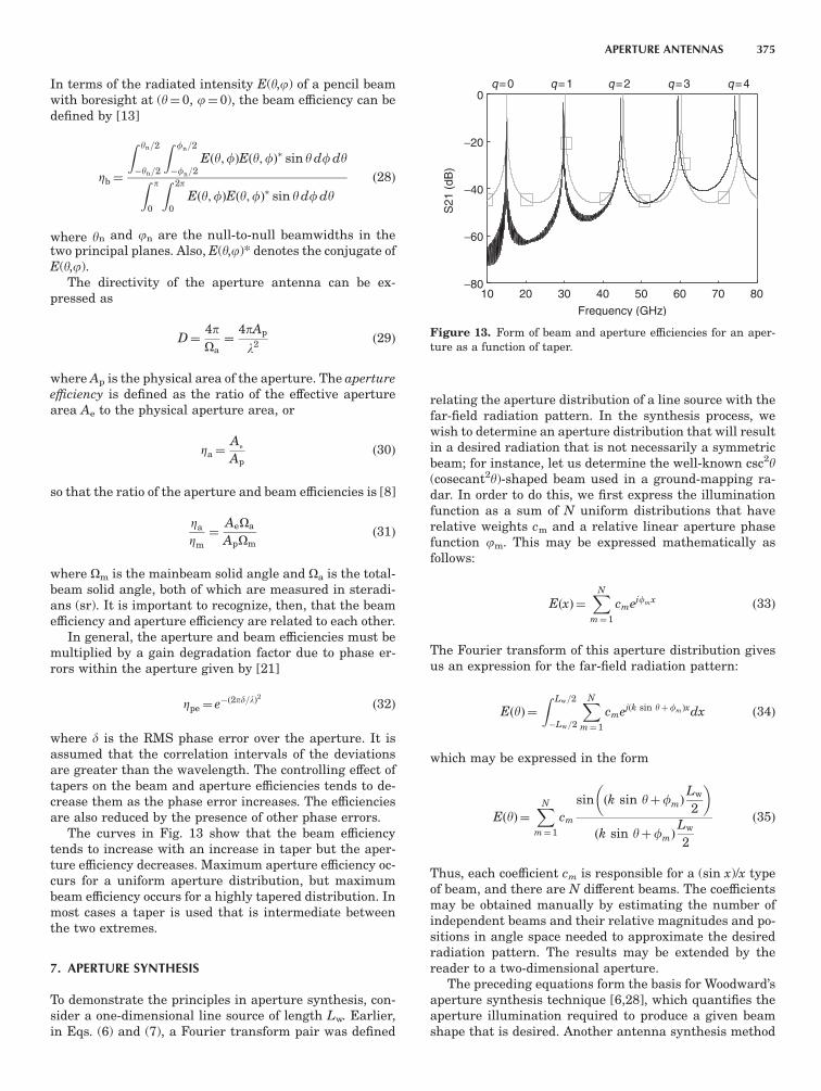
The curves in Fig. 13 show that the beam efficiencytends to increase with an increase in taper but the aper-ture efficiency decreases. Maximum aperture efficiency oc-curs for a uniform aperture distribution, but maximumbeam efficiency occurs for a highly tapered distribution. Inmost cases a taper is used that is intermediate betweenthe two extremes.

7. APERTURE SYNTHESIS

To demonstrate the principles in aperture synthesis, con-sider a one-dimensional line source of length Lw. Earlier,in Eqs. (6) and (7), a Fourier transform pair was defined

relating the aperture distribution of a line source with thefar-field radiation pattern. In the synthesis process, wewish to determine an aperture distribution that will resultin a desired radiation that is not necessarily a symmetricbeam; for instance, let us determine the well-known csc2y(cosecant2y)-shaped beam used in a ground-mapping ra-dar. In order to do this, we first express the illuminationfunction as a sum of N uniform distributions that haverelative weights cm and a relative linear aperture phasefunction jm. This may be expressed mathematically asfollows:

EðxÞ¼XN

m¼ 1

cmejfmx ð33Þ

The Fourier transform of this aperture distribution givesus an expression for the far-field radiation pattern:

EðyÞ¼Z Lw=2

�Lw=2

XN

m¼ 1

cmejðk sin yþfmÞxdx ð34Þ

which may be expressed in the form

EðyÞ¼XN

m¼ 1

cm

sin ðk sin yþfmÞLw

2

� �

ðk sin yþfmÞLw

2

ð35Þ

Thus, each coefficient cm is responsible for a (sin x)/x typeof beam, and there are N different beams. The coefficientsmay be obtained manually by estimating the number ofindependent beams and their relative magnitudes and po-sitions in angle space needed to approximate the desiredradiation pattern. The results may be extended by thereader to a two-dimensional aperture.

The preceding equations form the basis for Woodward’saperture synthesis technique [6,28], which quantifies theaperture illumination required to produce a given beamshape that is desired. Another antenna synthesis method

10 20 30 40 50 60 70 80

Frequency (GHz)

−80

−60

−40

−20

0

S21

(dB

)

q=0 q=1 q=2 q=3 q=4

Figure 13. Form of beam and aperture efficiencies for an aper-ture as a function of taper.


called the virtual array synthesis method was morerecently published by Vaskelainen [22]. In this method,the geometry of the virtual array is chosen so that therewill be a suitable synthesis method for that geometry, andthe synthesis of the virtual array can be done accurately.The excitation values for the virtual array are trans-formed into the excitation values of the actual array ge-ometry. Matrix operations are simple and large arrays caneasily be synthesized. Further information on antennapattern synthesis techniques is given in Refs. 23–27.

8. MODERN FULL-WAVE METHODS [29]

Some aperture antennas can be addressed with analysisapproaches known as full-wave methods. The applicationof such methods has rapidly expanded with the explosionof high-power PC computers.

Analysis methods are called ‘‘full-wave’’ when theystart with the fundamental equations of electromagneticsand discretize them such that they can be reduced to lin-ear matrix equations suitable for solving by a computer.The advantage is that there are no approximations inprinciple, only the size of the discrete interval, which isusually between 10 and 20 intervals per wavelength.There are three primary full-wave methods used in elec-tromagnetics: the finite-element method (FEM) [30–33],the method of moments (MoM) [34–36], and the finite-dif-ference time-domain (FDTD) method [37,38]. The MoMdiscretizes Maxwell’s wave equations in their integralform, the finite-difference method (FDM) discretizes theequations in the differential form, and the FEM methoddiscretizes the equations after casting them in a varia-tional form. All three techniques have been applied to ap-erture antenna analysis [39–41].

The MoM method finds natural application to antennasbecause it is based on surfaces and currents, whereas theother two methods are based on volumes and fields. Thismeans that for MoM, only the antenna aperture surfacestructure must be discretized and solved, whereas forFEM and FDTD, all volumes of interest must be discreti-zed. For antenna radiation, the far field would require aninordinate amount of space were it not for the recent de-velopment of absorbing boundary conditions. Theseboundary conditions approximate the radiation conditionsof infinite distance in the space very near the radiatingstructure.

The MoM works by solving for currents on all surfacesin the presence of a source current or field. The radiatedfield is then obtained by integration of these currents inmuch the same way as it was obtained in the physical op-tics (PO) approaches. Thus, the MoM can be applied to anyaperture antenna that the PO technique can be applied to,unless the problem is too large for the available computerresources. Ensemble [42] is a commercially available soft-ware package that is a 2.5D (two and one-half–dimension-al) MoM program used primarily for patch antennas orantennas that can be modeled as layers of dielectrics andconductors. If the top layer is a conductor with radiatingholes, the holes are aperture antennas, which this pro-gram is designed to analyze.

There is another full-wave commercial software pack-age that is widely used for aperture antenna problems: thehigh-frequency structure simulator (HFSS) [43]. This is a3D FEM software package with extensive modeling andautomatic meshing capability. It is best for horn antennasor other kinds of antennas formed by apertures in variousnonlayered structures. The latest version uses the ‘‘per-fectly matched layer’’ type of absorbing boundary condi-tions.

In practice, full-wave methods cannot be directly ap-plied to high-gain aperture antennas such as reflectors orlenses without difficulties because these structures areusually many wavelengths in size, requiring a largeamount of computational resources. Often, however, ifthere is symmetry in the problem that can be exploited,the number of unknowns for which to solve can be greatlyreduced. For instance, a high-gain reflector antenna thathas circular symmetry allows for body-of-revolution (BoR)symmetry [44,45] simplifications in the modeling. Simi-larly, a large lens requires a computer program with di-electric capability [46] in addition to BoR symmetrymodeling.

BIBLIOGRAPHY

1. D. J. Kozakoff, Analysis of Radome Enclosed Antennas, ArtechHouse, Norwood, MA, 1997.

2. S. A. Schelkunoff, Some equivalence theorems of electromag-netics and their application to radiation problems, Bell Syst.Tech. J., 15:92–112 (1936).

3. C. Huygens, Traite de La Lumiere, Leyden, 1690 (transl. intoEnglish by S. P. Thompson, Chicago, IL, Univ. Chicago Press,1912).

4. J. D. Kraus and D. Fleisch, Electromagnetics, 5th ed.,McGraw-Hill, New York, 1998.

5. C. A. Balinis, Antenna Theory Analysis and Design, Harper &Row, New York, 1982.

6. A. D. Oliver, Basic properties of antennas, in A. W. Rudge etal., eds., The Handbook of Antenna Design, IEE Electromag-netic Wave Series, Peter Peregrinus, Stevanage, UK, 1986,Chapter 1.

7. H. Jasik, Fundamentals of antennas, in R. C. Johnson, ed.,Antenna Engineering Handbook, 3rd ed., McGraw-Hill, NewYork, 1993.

8. J. D. Kraus, Antennas, 2nd ed., McGraw-Hill, New York,1988.

9. A. Sommerfeld, Theorie der Beugung, in P. Frank and R.vonMises, eds., Die Differential und Integralgleichungen der Me-

chaniik und Physik, Vieweg, Braunschweig, Germany, 1935.

10. J. D. Kraus, Radio Astronomy, 2nd ed., Cygnus-Quasar Pub-lishers, New York, 1956.

11. R. E. Collin and Z. J. Zucker, Antenna Theory, McGraw-Hill,New York, 1969.

12. W. L. Weeks, Antenna Engineering, McGraw-Hill, New York,1968.

13. T. A. Milligan, Modern Antenna Design, McGraw-Hill, NewYork, 1985.

14. A. W. Rudge et al., The Handbook of Antenna Design, PeterPeregrinus, Stevanage, UK, 1986.

15. S. Silver, Microwave Antenna Theory and Design, McGraw-Hill, New York, 1949.


16. H. G. Booker and P. C. Clemmow, The concept of an angularspectrum of plane waves and its relation to that of polardiagram and aperture distribution, Proc. IEEE 97:11–17(1950).

17. D. R. Rhodes, The optimum line source for the best meansquare approximation to a given radiation pattern, IEEE

Trans. Anten. Propag. AP-11:440–446 (1963).

18. R. S. Elliot, Antenna Theory and Design, Prentice-Hall,Englewood Cliffs, NJ, 1987.

19. I. S. Sokolnikoff and R. M. Redhefer, Mathematics of

Physics and Modern Engineering, McGraw-Hill, New York,1958.

20. R. C. Hansen, Linear arrays, in A. W. Rudge et al., eds., The

Handbook of Antenna Design, Peter Peregrinus, Stevanage,UK, 1986.

21. R. T. Nash, Beam efficiency limitations for large antennas,IEEE Trans. Anten. Propag. AP-12:918–923 (1964).

22. L. I. Vaskelainen, Virtual array synthesis method for planararray antennas, IEEE Trans. Anten. Propag. 46:922–928(1998).

23. R. J. Mailoux, Phased Array Antenna Handbook, ArtechHouse, Norwood, MA, 1994.

24. E. Botha and D. A. McNamara, A contoured beam synthesistechnique for planar antenna arrays with quadrantal andcentro-symmetry, IEEE Trans. Anten. Propag. 41:1222–1231(1993).

25. B. P. Ng, M. H. Er, and C. Kot, A flexible array synthesismethod using quadratic programming, IEEE Trans. Anten.

Propag. 41:1541–1550 (1993).

26. H. J. Orchard, R. S. Elliot, and G. J. Stern, Optimizing thesynthesis of shaped beam antenna patterns, IEEE Proc.132(1):63–68 (1985).

27. R. F. E. Guy, General radiation pattern synthesis techniquefor array antennas of arbitrary configuration and elementtype, Proc. IEEE 135(4):241–248 (1988).

28. P. M. Woodward, A method of calculating the field over aplane aperture required to produce a given polar diagram,IEEE J. 93:1554–1558 (1947).

29. V. Tripp, Full Wave Methods for Analysis of Aperture Anten-

nas, USDigiComm Corp., Stone Mountain, GA, 2003.

30. J. L. Volakis, A. Chatterjee, and L. C. Kempel, Finite Element

Methods for Electromagnetics, IEEE Press, New York andOxford Univ. Press, London, 1998.

31. P. P. Sylvester, G. Pelosi, ed., Finite Elements for Wave Elec-

tromagnetics: Methods and Techniques, IEEE Press, NewYork, 1994.

32. P. P. Sylvester and R. L. Ferrari, Finite Elements for Electrical

Engineers, Cambridge Univ. Press, New York, 1992.

33. J. Jin, The Finite Element Method in Electromagnetics, Wiley-Interscience, New York, 1993.

34. R. F. Harrington, Field Computation by Moment Methods,Macmillan, New York, 1968.

35. E. K. Miller, L. Medgyesi-Mitschang, and E. H. Newman,eds., Computational Electromagnetics, Frequency Domain

Method of Moments, IEEE Press, New York, 1992.

36. R. C. Hansen, ed., Moment Methods in Antennas and Scat-

tering, Artech House, Norwood, MA, 1990.

37. A. Taflove, Computational Electromagnetics: The FiniteDifference Time Domain Method, Artech House, Norwood,MA, 1995.

38. K. S. Kunz and R. J. Luebbers, The Finite Difference Time

Domain Method for Electromagnetics, CRC Press, Cleveland,OH, 1993.

39. D. Chun, R. N. Simons, and L. P. B. Kotehi, Modeling andcharacterization of cavity backed circular aperture antennawith suspended stripline probe feed, IEEE Antennas Propa-

gation Soc. Int. Symp. 2000 Digest, Salt Lake City, UT, 2000.

40. J. Y. Lee, T. S. Horng, and N. G. Alexopoulos, Analysis of cav-ity backed aperture antennas with a dielectric overlay, IEEETrans. Anten. Propag. 42(11):1556–1562 (Nov. 1994).

41. D. Sullivan and J. L. Young, Far-field time-domain calculationfrom aperture radiators using the FDTD method, IEEE

Trans. Anten. Propag. 49(3), 464–469 (March 2001).

42. Ensemble Software, version 6.1, Ansoft Corp., Four StationSquare, Suite 200, Pittsburgh, PA 15219, Tel: 412-261-3200.

43. Ansoft Corp., Four Station Square, Suite 200, Pittsburgh, PA15219, Tel: 412-261-3200.

44. Z. Altman and R. Mittra, Combining an extrapolation tech-nique with the method of moments for solving large scatter-ing problems involving bodies of revolution, IEEE Trans.

Anten. Propag. 44(4), 548–553 (April 1996).

45. A. D. Greenwood and J. M. Jin, Finite element analysis ofcomplex axisymmetric radiating structures, IEEE Trans.Anten. Propag. 47(8), 1260 (Aug. 1999).

46. J. M. Putnam and L. N. Medgyesi-Mitschang, Combined fieldintegral equation for inhomogeneous two- and three-dimen-sional bodies: The junction problem, IEEE Trans. Anten.Propag. 39(5), 667–672 (May 1991).

FURTHER READING

C. A. Balanis, Antenna Theory Analysis and Design, Harper &Row, New York, 1982.

E. T. Bayliss, Design of monopulse difference patterns with lowsidelobes, Bell Syst. Tech. J. 47, 623–650 (1968).

R. N. Bracewell, Tolerance theory of large antennas, IRE Trans.Anten. Propag. AP-9, 49–58 (1961).

W. N. Christiansen and J. A. Hogbom, Radiotelescopes, Cam-bridge Univ. Press, Cambridge, UK, 1985.

APPLICATION OF WAVELETS TOELECTROMAGNETIC PROBLEMS

JAIDEVA C. GOSWAMI

Schlumberger TechnologyCorporation

Sugar Land, Texas

MANOS M. TENTZERIS

Georgia Institute of TechnologyAtlanta, Georgia

1. INTRODUCTION

Since the early nineteenth century, Fourier analysis hasplayed an important role in almost all branches of scienceand engineering and in some areas of social science aswell. In this method a function is transformed from onedomain to another where many characteristics of thefunction are revealed. One usually refers to this transform

APPLICATION OF WAVELETS TO ELECTROMAGNETIC PROBLEMS 377

domain as the spectral, frequency, or wavenumber domain,while the original domain is referred to as time or spatialdomain. In many applications, combined time–frequencyanalysis of a signal provides useful information about thephysical phenomena; information that could not be ex-tracted by either the time-domain or the frequency-do-main analyses. For instance, in applications toidentification and classification of targets based on theanalysis of radar echo, time-domain scattering centeranalysis [1,2] provides information about the local fea-tures of the scatterer since these features appear as shorttimepulses. Frequency-domain analysis of radar echousing the singularity expansion method [3,4] providesinformation about the global features of the target. Thecombined time–frequency analysis can provide additionalinformation, such as the dispersive nature of the target[5,6] and the dispersive nature of propagation in a trans-mission line [7].

Another area of interest to the electromagneticscommunity concerns solving boundary value problemsarising from scattering and propagation of electromag-netic waves. Two of the main properties of waveletsvis-a-vis boundary value problems are their hierarchicalnature and the vanishing moments properties. Because oftheir hierarchical (multiresolution) nature, waveletsat different resolutions (scales) are interrelated, a prop-erty that makes them suitable candidates for multigrid-type methods for solving partial-differential equations.On the other hand, the vanishing-moment property,causing wavelets, when integrated against a function ofcertain order, to render the integral zero, is attractive insparsifying a dense matrix generated by an integralequation.

In applications to discrete datasets, wavelets may beconsidered as basis functions generated by dilations andtranslations of a single function. Analogous to Fourieranalysis, there are wavelet series (WS) and integralwavelet transforms (IWTs). In wavelet analysis, WS andIWT are intimately related. The IWT of a finite-energyfunction on the real line evaluated at certain points inthe timescale domain gives the coefficients for itswavelet series representation. No such relation existsbetween Fourier series and Fourier transform, which areapplied to different classes of functions; the former isapplied to finite-energy periodic functions, whereas thelatter is applied to functions that have finite energy overthe real line. Furthermore, Fourier analysis is global inthe sense that each frequency (time) component ofthe function is influenced by all the time (frequency)components of the function. On the other hand, waveletanalysis is a local analysis. This local nature of waveletanalysis makes it suitable for time–frequency analysis ofsignals.

Wavelet techniques enable us to divide a complicatedfunction into several simpler ones and study them sepa-rately. This property, along with fast wavelet algorithmsthat are comparable in efficiency to fast Fourier transformalgorithms, makes these techniques very attractive inanalysis and synthesis problems.

In this article we discuss some wavelet applications toelectromagnetic problems. The organization of this article

is as follows. In the next section we give an overview ofwavelet theory. Sections 3 to 6 deal with solution ofintegral equations arising from electromagnetic scatteringand transmission-line problems. Differential equations,especially the multiresolution time-domain method, areconsidered in Section 7. Readers may refer to the litera-ture [5–7] for time-frequency analysis of electromagneticdata.

2. WAVELET PRELIMINARIES

In this section we briefly describe the basics of wavelettheory to facilitate subsequent discussion on its applica-tion. More details on the topic may be found in theliterature [8–16].

2.1. Multiresolution Analysis

As pointed out before, multiresolution analysis (MRA)plays an important role in the application of wavelets toboundary value problems. In order to achieve MRA wemust have a finite-energy function (square integrable onthe real line) fðxÞ 2 L2ðRÞ, called a scaling function, thatgenerates a nested sequence of subspaces

f0g V�1 V0 V1 ! L2 ð1Þ

and satisfies the dilation (refinement) equation, namely

fðxÞ¼X

k

pkfð2x� kÞ ð2Þ

with {pk} belonging to the set of square summable biinfi-nite sequences. The number 2 in (2) signifies ‘‘octavelevels.’’ In fact, this number could be any rational number,but we will discuss only octave levels or scales. From (2)we see that the function f(x) is obtained as a linearcombination of a scaled and translated version of itself,and hence the term scaling function.

The subspaces Vj are generated by fj;kðxÞ :¼2j=2fð2jx� kÞ; j, k 2 Z, where Z :¼f. . . ;�1; 0; 1; . . .g. Foreach scale j, since Vj Vjþ 1, there exists a complementarysubspace Wj of Vj in Vjþ 1. This subspace Wj, called‘‘wavelet subspace,’’ is generated by cj;kðxÞ :¼ 2j=2cð2jx� kÞ, where cAL2 is called the ‘‘wavelet.’’ From thediscussion above, these results follow easily:

Vj1 [Wj1¼Vj2 j2¼ j1þ 1

Vj1 \ Vj2¼Vj2 j1 > j2

Wj1 \Wj2¼f0g j1Oj2

Vj1 \Wj2¼f0g j1 � j2

8>>>>><

>>>>>:

ð3Þ

The scaling function f exhibits lowpass filter character-istics in the sense that ffð0Þ¼ 1, where a hat over thefunction denotes its Fourier transform. On the other hand,the wavelet function c exhibits bandpass filter character-istic in the sense that ccð0Þ¼ 0. Later in the article, we willsee some examples of wavelets and scaling functions.

378 APPLICATION OF WAVELETS TO ELECTROMAGNETIC PROBLEMS

2.2. Properties of Wavelets

Some of the important properties that we will discuss inthis article are given below:

* Vanishing moment—a wavelet is said to have avanishing moment of order m if

Z 1

�1

xpcðxÞdx¼ 0; p¼ 0; . . . ;m� 1 ð4Þ

All wavelets must satisfy this condition for p¼ 0.* Orthonormality—the wavelets {cj,k} form an ortho-

normal basis if

hcj;k;cl;mi¼ dj;ldk;m; for all j; k; l;m 2 Z ð5Þ

where dp,q is the Kronecker delta defined in the usualway as

dp;q¼1 p¼ q

0 otherwise

(ð6Þ

The inner product /f1, f2S of two square integrablefunctions f1 and f2 is defined as

hf1; f2i : ¼

Z 1

�1

f1ðxÞf�2 ðxÞdx

with f �2 ðxÞ, representing the complex conjugation of f2.* Semiorthogonality—The wavelets {cj,k} form a semi-

orthogonal basis if

hcj;k;cl;mi¼ 0; jOl; for all j;k; l;m 2 Z ð7Þ

2.3. Wavelet Transform Algorithm

Given a function f(x)AL2, the decomposition into variousscales begins by mapping the function into a sufficientlyhigh-resolution subspace VM:

L23f ðxÞ7!fM ¼X

k

aM;kfð2Mx� kÞ 2 VM ð8Þ

Now since

VM ¼WM�1þVM�1

¼WM�1þWM�2þVM�2

¼XN

n¼1

WM�nþVM�N ;

ð9Þ

we can write

fMðxÞ ¼XN

n¼ 1

gM�nðxÞþ fM�NðxÞ ð10Þ

where fM�N(x) is the coarsest approximation of fM(x) and

fjðxÞ ¼X

k

aj;kfð2jx� kÞ 2 Vj ð11Þ

gjðxÞ¼X

k

wj;kcð2jx� kÞ 2 Wj ð12Þ

If the scaling functions and wavelets are orthonormal, itis easy to obtain the coefficients {aj,k} and {wj,k}. Howeverfor the semiorthogonal case, we need a dual scalingfunction ð ~ffÞ and dual wavelet ð ~ccÞ. Dual wavelets satisfythe ‘‘biorthogonality condition’’:

hcj;k; ~ccl;mi¼ dj;l dk;m; j; k; l;m 2 Z ð13Þ

For the semiorthogonal case, both c and ~cc belong to thesame space Wj for an appropriate j; likewise f and ~ffbelong to Vj. One difficulty with semiorthogonal waveletsis that their duals do not have compact support. We canachieve compact support for both ~ff and ~cc if we forgo theorthogonality requirement that Vj>Wj. In such a case weget ‘‘biorthogonal wavelets’’ [17] and two MRAs, {Vj} andf ~VVjg. In this article we will discuss application of ortho-normal and semiorthogonal wavelets only.

3. INTEGRAL EQUATIONS

Integral equations appear frequently in practice, particu-larly the first-kind integral equations [18] in inverseproblems. These equations can be represented as

LKf ¼

Z b

a

f ðx0ÞKðx; x0Þdx0 ¼ gðxÞ ð14Þ

where f(x) is an unknown function, K(x, x0) is the knownkernel that might be the system impulse response orGreen’s function, and g(x) is the known response function.

3.1. Electromagnetic Scattering

Consider the problem of electromagnetic scattering by aninfinitely long metallic cylinder, as shown in Fig. 1. Forsuch a problem, electric surface current Jsz is related tothe incident electric field via an integral equation

jom0

Z

C

Jszðl0ÞGðl; l0Þdl0 ¼Ei

zðlÞ ð15Þ

where

Gðl; l0Þ ¼1

4jHð2Þ0 ðk0jrðlÞ � rðl0ÞjÞ ð16Þ

with the wavenumber k0¼ 2p/l0. The electric field Eiz is

the z component of the incident electric field and Hð2Þ0 is thesecond-kind Hankel function of order 0, and l0 is thewavelength in free space. Here, the contour of integrationhas been parameterized with respect to the chord length.


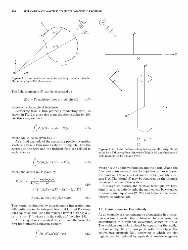
The field component Eiz can be expressed as

EizðlÞ¼E0 exp½jk0ðxðlÞ cosfiþ yðlÞ sinfiÞ� ð17Þ

where fi is the angle of incidence.Scattering from a thin perfectly conducting strip, as

shown in Fig. 2a, gives rise to an equation similar to (15).For this case, we have

Z h

�h

Jsyðz0ÞGðz; z0Þdz0 ¼Ei

yðzÞ ð18Þ

where G(z, z0) is as given by (16).As a final example of the scattering problem, consider

scattering from a thin wire as shown in Fig. 2b. Here thecurrent on the wire and the incident field are related toeach other as

Z l

�l

Iðz0ÞKwðz; z0Þdz0 ¼ � EiðzÞ ð19Þ

where the kernel Kw is given by

Kwðz; z0Þ ¼

1

4pjoe0

expð�jk0RÞ

R5

� ½ð1þ jk0RÞ� ð2R2 � 3a2Þ þk20a2R2�

ð20Þ

EiðzÞ¼E0 sin y exp ðjk0z cos yÞ ð21Þ

This kernel is obtained by interchanging integration anddifferentiation in the integrodifferential form of Pockling-ton’s equation and using the reduced kernel distance R¼[a2þ (z� z0)2]1/2, where a is the radius of the wire [19].All the equations described thus far have the form of a

first-kind integral equation, namely

Z b

a

f ðx0ÞKðx; x0Þdx0 ¼ gðxÞ ð22Þ

where f is the unknown function and the kernel K and thefunctions g are known. Here the objective is to reconstructthe function f from a set of known data (possibly mea-sured) g. The kernel K may be regarded as the impulseresponse function of the system.

Although we discuss the solution technique for first-kind integral equations only, the method can be extendedto second-kind equations [20,21] and higher-dimensionalintegral equations [22].

3.2. Transmission-Line Discontinuity

As an example of electromagnetic propagation in a trans-mission line, consider the problem of characterizing onediscontinuity of a coplanar waveguide, shown in Fig. 3.The problem can be formulated by separating the config-uration of Fig. 3a into two parts with the help of theequivalence principle [23], according to which the slotregions can be replaced by equivalent surface magnetic

n

�(l )

XZ

Y

Ezi

�(l ′)

l

C

�i

l∧

∧

Figure 1. Cross section of an infinitely long metallic cylinderilluminated by a TM plane wave.

Ei

Ei

X

(a)

(b)

Z

Z

X

Y

2a

Figure 2. (a) A thin half-wavelength-long metallic strip illumi-nated by a TM wave; (b) a thin wire of length l/2 and thickness l/1000 illuminated by a plane wave.


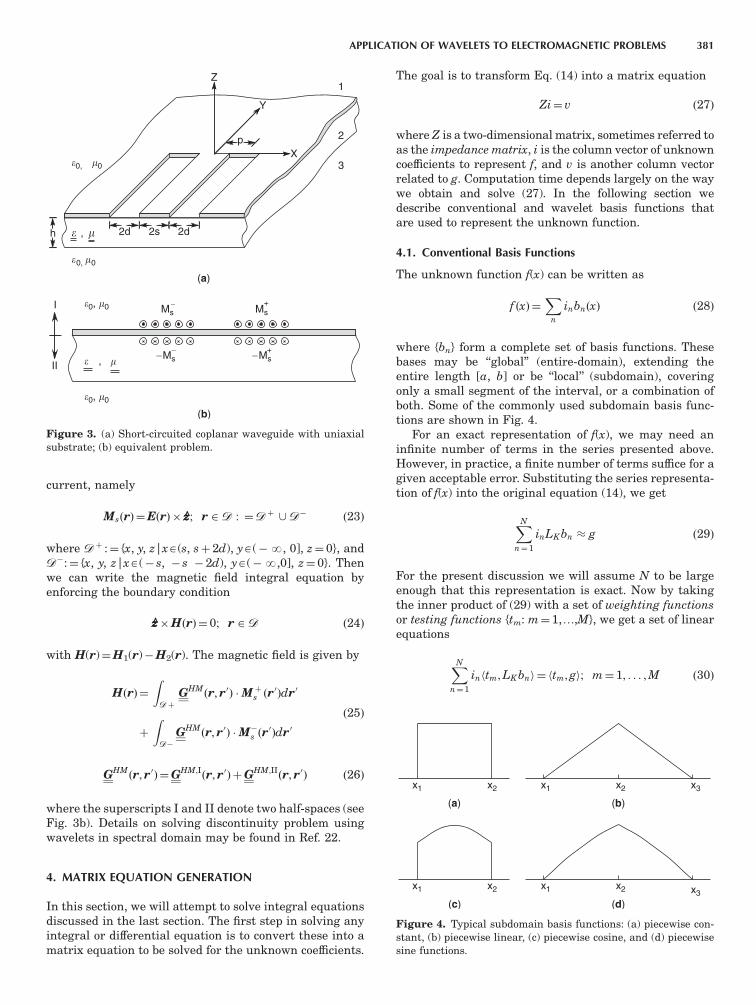
current, namely

MsðrÞ¼EðrÞ� zz; r 2 D : ¼Dþ [D� ð23Þ

where Dþ :¼ {x, y, z|xA(s, sþ 2d), yA(�N, 0], z¼ 0}, andD�:¼ {x, y, z|xA(� s, � s � 2d), yA(�N,0], z¼ 0}. Thenwe can write the magnetic field integral equation byenforcing the boundary condition

zz�HðrÞ¼ 0; r 2 D ð24Þ

with H(r)¼H1(r)�H2(r). The magnetic field is given by

HðrÞ¼

Z

Dþ

GHMðr; r0Þ M þ

s ðr0Þdr0

þ

Z

D�

GHMðr; r0Þ M�s ðr

0Þdr0ð25Þ

GHMðr; r0Þ ¼GHM;I

ðr; r0Þ þGHM;IIðr; r0Þ ð26Þ

where the superscripts I and II denote two half-spaces (seeFig. 3b). Details on solving discontinuity problem usingwavelets in spectral domain may be found in Ref. 22.

4. MATRIX EQUATION GENERATION

In this section, we will attempt to solve integral equationsdiscussed in the last section. The first step in solving anyintegral or differential equation is to convert these into amatrix equation to be solved for the unknown coefficients.

The goal is to transform Eq. (14) into a matrix equation

Zi¼ v ð27Þ

where Z is a two-dimensional matrix, sometimes referred toas the impedance matrix, i is the column vector of unknowncoefficients to represent f, and v is another column vectorrelated to g. Computation time depends largely on the waywe obtain and solve (27). In the following section wedescribe conventional and wavelet basis functions thatare used to represent the unknown function.

4.1. Conventional Basis Functions

The unknown function f(x) can be written as

f ðxÞ ¼X

n

inbnðxÞ ð28Þ

where {bn} form a complete set of basis functions. Thesebases may be ‘‘global’’ (entire-domain), extending theentire length [a, b] or be ‘‘local’’ (subdomain), coveringonly a small segment of the interval, or a combination ofboth. Some of the commonly used subdomain basis func-tions are shown in Fig. 4.

For an exact representation of f(x), we may need aninfinite number of terms in the series presented above.However, in practice, a finite number of terms suffice for agiven acceptable error. Substituting the series representa-tion of f(x) into the original equation (14), we get

XN

n¼ 1

inLKbn � g ð29Þ

For the present discussion we will assume N to be largeenough that this representation is exact. Now by takingthe inner product of (29) with a set of weighting functionsor testing functions {tm: m¼ 1,y,M}, we get a set of linearequations

XN

n¼1

inhtm;LKbni¼ htm; gi; m¼ 1; . . . ;M ð30Þ

�0, �0

Z

X

Y

2

1

3

, 2d 2s 2d

p

�0, �0

� �h

(a)

−

Ms

,� �

�0, �0

�0, �0

+Ms

+

I

II

−

−Ms −Ms

(b)

Figure 3. (a) Short-circuited coplanar waveguide with uniaxialsubstrate; (b) equivalent problem.

x1 x2 x1 x2 x3

(a) (b)

(c) (d)

x1 x2 x1 x2 x3

Figure 4. Typical subdomain basis functions: (a) piecewise con-stant, (b) piecewise linear, (c) piecewise cosine, and (d) piecewisesine functions.


which can be written in the matrix form as

½Zmn�½in� ¼ ½vm� ð31Þ

where

Zmn¼htm;LKbni; m¼ 1; . . . ;M; n¼ 1; . . . ;N

vm¼htm; gi; m¼ 1; . . . ;M

The solution of the matrix equation gives the coefficients{in} and thereby the solution of the integral equations. Twomain choices of the testing functions are (1) tm(x)¼d(x� xm), where xm is a discretization point in the domain;and (2) tm(x)¼ bm(x). In the former case the method iscalled point matching, whereas the latter method isknown as the Galerkin method. The method so describedand those to be discussed in the following sections aregenerally referred to as ‘‘method of moments’’ (MoM) [24].We will call MoM with conventional bases as ‘‘conven-tional MoM’’ and the method with wavelet bases, ‘‘waveletMoM.’’ Observe that the operator LK in the precedingparagraphs could be any linear operator—differential aswell as integral.

4.2. Wavelet Bases

Conventional bases (local or global), when applied directlyto the integral equations, generally lead to a dense (fullypopulated) matrix Z. As a result, the inversion and thefinal solution of such a system of linear equations are verytime-consuming. In later sections it will be clear whyconventional bases give a dense matrix while waveletbases produce sparse matrices. Observe that conventionalMoM is a single-level approximation of the unknownfunction in the sense that the domain of the function(e.g., [a, b]), is discretized only once, even if we usenonuniform discretization of the domain. Wavelet MoMas we will discuss, on the other hand, is inherently multi-level in nature.

Beylkin et al. [25] first proposed the use of wavelets insparsifying an integral equation. Alpert et al. [20] used‘‘waveletlike’’ basis functions to solve second-kind integralequations. In electrical engineering, wavelets have beenused to solve integral equations arising from electromag-netic scattering and transmission-line problems [22,26–40]. In what follows we briefly describe four different waysin which wavelets have been used in solving integralequations.

4.2.1. Use of Fast Wavelet Algorithm. In this method,the impedance matrix Z is obtained via the conventionalmethod of moments using basis functions such as trian-gular functions, and then wavelets are used to transformthis matrix into a sparse matrix [26,27]. Consider a matrixW formed by wavelets. This matrix consists of the decom-position and reconstruction sequences and their trans-lates. We have not discussed these sequences here, but

readers may find these sequences in any standard book onwavelets [e.g., 8–16].

Transformation of cite original MoM impedance matrixinto the new wavelet basis is obtained as

WZWT . ðWTÞ�1i¼Wv ð32Þ

which can be written as

Zw . iw¼ vw ð33Þ

where WT represents the transpose of the matrix W. Thenew set of wavelet-transformed linear equations are

Zw¼WZWT ð34Þ

iw¼ ðWTÞ�1i ð35Þ

vw¼Wv ð36Þ

The solution vector i is then given by

i¼WTðWZWTÞ�1Wv ð37Þ

For orthonormal wavelets WT¼W� 1 and the trans-

formation (32) is ‘‘unitary similar.’’ It has been shown[26,27] that the impedance matrix Zw is sparse, winchreduces the inversion time significantly. Discrete wavelettransform (DWT) algorithms can be used to obtain Zw.Readers may find the details of discrete wavelet transform(octave scale transform) in any standard book on wavelets.In some applications it may be necessary to computethe wavelet transform at nonoctave scales. Readers arereferred to the literature [7,41,42] for details on suchalgorithms.

4.2.2. Direct Application of Wavelets. In anothermethod of applying wavelets to integral equations, wave-lets are directly applied; that is, first the unknown func-tion is represented as a superposition of wavelets atseveral levels (scales) along with the scaling function atthe lowest level, prior to using Galerkin’s method de-scribed before.

In terms of wavelets and scaling functions we can writethe unknown function f in (14) as

f ðxÞ¼Xju

j¼ j0

XKðjÞ

k¼K1

wj;k cj;kðxÞ

þXKðj0Þ

k¼K1

aj0 ;k fj0 ;kðxÞ

ð38Þ

where we have used the multiscale property (10).It should be pointed out here that the wavelets {cj,k} by

themselves form a complete set; therefore, the unknownfunction could be expanded entirely in terms of the wave-lets. However, to retain only a finite number of terms inthe expansion, the scaling function part of (38) must beincluded. In other words, {cj,k}, because of their bandpass


filter characteristics, extract successively lower and lowerfrequency components of the unknown function withdecreasing values of the scale parameter j, while fj0 ;k,because of its lowpass filter characteristics, retains thelowest frequency components or the coarsest approxima-tion of the original function.

In Eq. (38), the choice of j0 is restricted by the order ofthe wavelet, while the choice of ju is governed by thephysics of the problem. In applications involving electro-magnetic scattering, as a ‘‘rule of thumb’’ the highestscale, ju, should be chosen such that 1=2ju þ 1 does notexceed 0.1l0, where l0 is the operative wavelength.

When (38) is substituted in (14), and the resultantequation is tested with the same set of expansion func-tions, we get a set of linear equations

½Zf;f� ½Zf;c�

½Zc;f� ½Zc;c�

" #½aj0 ;k�k

½wj;n�j;n

" #¼hv;fj0 ;k 0 ik 0

hv;cj 0 ;k 0 ij 0 ;k 0

" #ð39Þ

where the c term of the expansion function and the f termof the testing function give rise to the [Zf,c] portion of thematrix Z. A similar interpretation holds for [Zf,f], [Zc,f],and [Zc,c].

By carefully observing the nature of the submatrices,we can explain the ‘‘denseness’’ of the conventional MoMand the ‘‘sparseness’’ of the wavelet MoM. Unlike wave-lets, the scaling functions discussed in this article do notposses the vanishing moments properties. Consequently,for two pulse or triangular functions f1 and f2 (usualbases for the conventional MoM and suitable candidatesfor the scaling functions), even though /f1, f2S¼ 0for nonoverlapping support, /f1, LKf2S is not verysmall since Lkf2 is not small. On the other hand, as isclear from the vanishing-moment property (4) of a waveletof order m, the integral vanishes if the function againstwhich the wavelet is being integrated behaves as a poly-nomial of a certain order ‘‘locally.’’ Away from the singularpoints the kernel has a polynomial behavior locally.Consequently, integrals such as (LKcj,n) and the innerproducts involving wavelets are very small for nonover-lapping support.

Because of its ‘‘total positivity’’ property [11, pp. 207–209], the scaling function has a ‘‘smoothing’’ or ‘‘variationdiminishing’’ effect on a function against which it isintegrated. The smoothing effect can be understood asfollows. If we convolve two pulse functions, both of whichare discontinuous but totally positive, the resultant func-tion is a linear B-spline (triangular function) that iscontinuous. Likewise, if we convolve two linear B-splines,we get a cubic B-spline that is twice continuously differ-entiable. Analogous to these, the function LKfj0 ;k issmoother than the kernel K itself. Furthermore, becauseof the MRA properties that give

hfj;k;cj 0 ;li¼ 0; j � j0 ð40Þ

the integrals hfj0 ;k 0 ; ðLKcj;nÞi and hcj 0 ;n 0 ; ðLKfj0 ;kÞi are quitesmall.

The [Zf,f] portion of the matrix, although diagonallydominant, usually does not have entries that are very

small compared to the diagonal entries. In conventionalMoM case, all the elements of the matrix are of the form/fj,k0,(LKfj,k)S. Consequently, we cannot, threshold sucha matrix in order to sparsify it. In wavelet MoM case, theentries of [Zf,f] occupy a very small portion (5 � 5 forlinear and 11 � 11 for cubic spline cases) of the matrix,while the rest contain entries whose magnitudes are verysmall compared to the largest, entry; hence a significantnumber of entries can be set to zero without affecting thesolution appreciably.

4.2.3. Wavelets in Spectral Domain. In the previoussection, we have used wavelets in the space domain. Thelocal support and vanishing-moment properties of waveletbases were used to obtain a sparse matrix representationof an integral equation. In some applications, particularlyin spectral-domain methods in electromagnetics, waveletsin the spectral domain may be quite useful. Whenever wehave a problem in which the unknown function is ex-panded in terms of the basis function in the space (time)domain while the numerical computation takes place inthe spectral (frequency) domain, we should look at thespace–spectral window product in order to determine theefficiency of using a particular basis function. According tothe ‘‘uncertainty principle,’’ the space–spectral windowproduct of a square integrable function cannot be lessthan 0.5; the lowest value is possible only for functions ofGaussian class. Because of the nearly optimal space–spectral window product of the cubic spline and thecorresponding semiorthogonal wavelet, the improper in-tegrals appearing in many spectral-domain formulationsof integral equations can be evaluated efficiently. This isdue to the fact that higher-order wavelets generally havefaster decay in the spectral domain. The spectral-domainwavelets have been used to solve the transmission-linediscontinuity problem [22].

4.2.4. Wavelet Packets. The discrete wavelet packet(DWP) similarity transformation has been used to obtaina higher degree of sparsification of the matrix than isachievable using the standard wavelets [38]. It has alsobeen shown that the DWP method gives faster matrix-vector multiplication than do some of the fast multipolemethods.

In the standard wavelet decomposition process, first wemap the given function to a sufficiently high-resolutionsubspace (VM) and obtain the approximation coefficients{aM,k} (see Section 2). The approximation coefficients{aM� 1,k} and wavelet coefficients {wM� 1,k} are computedfrom {aM,k}. This process continues; that is, the coefficientsfor the next-lower level M� 2 are obtained from {aM� 1,k},and so on. Observe that in this scheme, only approxima-tion coefficients {aj,k} are processed at any scale j; thewavelet coefficients are merely the outputs and remainuntouched. In a wavelet packet, the wavelet coefficientsare also processed, which, heuristically, should result in ahigher degree of sparsity since in this scheme, the fre-quency bands are further divided compared with thestandard decomposition scheme.


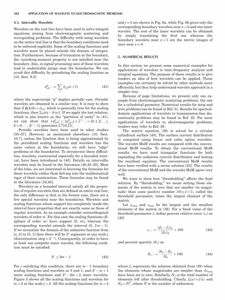
4.3. Intervallic Wavelets

Wavelets on the real line have been used to solve integralequations arising from electromagnetic scattering andwaveguiding problems. The difficulty with using waveletson the entire real line is that the boundary conditions needto be enforced explicitly. Some of the scaling functions andwavelets must be placed outside the domain of integra-tion. Furthermore, because of truncation at the boundary,the vanishing-moment property is not satisfied near theboundary. Also, in signal processing uses of these waveletslead to undesirable jumps near the boundaries. We canavoid this difficulty by periodizing the scaling function as[10, Sect. 9.3]

fpj;k : ¼

X

l

fj;kðxþ lÞ ð41Þ

where the superscript ‘‘p’’ implies periodic case. Periodicwavelets are obtained in a similar way. It is easy to showthat if ffð2pkÞ¼ dk;0, which is generally true for the scalingfunctions, then Skf(x� k)�1. If we apply the last relation,which is also known as the ‘‘partition of unity’’ to (41),we can show that ffp

0;0g [ fcpj;k; j 2 Zþ : ¼f0; 1; 2; . . .g;

k¼ 0; . . . ; 2 j � 1g generates L2([0,1]).Periodic wavelets have been used in other studies

[35–37]. However, as mentioned elsewhere [10, Sect.10.7], unless the function that is being approximated bythe periodized scaling functions and wavelets has thesame values at the boundaries, we still have ‘‘edge’’problems at the boundaries. To circumvent these difficul-ties, wavelets, constructed especially for a bounded inter-val, have been introduced in [40]. Details on intervallicwavelets may be found in the literature [40,43–45]. Mostof the time, we are interested in knowing the formulas forthese wavelets rather than delving into the mathematicalrigor of their construction. These formulas may be foundin the literature [16,40].

Wavelets on a bounded interval satisfy all the proper-ties of regular wavelets that are defined on entire real line;the only difference is that in the former case, there are afew special wavelets near the boundaries. Wavelets andscaling functions whose support lies completely inside theinterval have properties that are exactly same as those ofregular wavelets. As an example consider semiorthogonalwavelets of order m. For this case the scaling functions (B-splines of order m) have support [0, m], whereas thecorresponding wavelet extends the interval [0, 2 m� 1].If we normalize the domain of the unknown function from[a, b] to [0, 1] then there will be 2 j segments at any scale j(discretization step¼ 2� j). Consequently, in order to haveat least one complete inner wavelet, the following condi-tion must be satisfied:

2 j � 2m� 1 ð42Þ

For j satisfying this condition, there are m� 1 boundaryscaling functions and wavelets at 0 and 1, and 2 j

�mþ 1inner scaling functions and 2 j

� 2mþ 2 inner wavelets.Figure 5 shows all the scaling functions and wavelets form¼ 2 at the scale j¼ 2. All the scaling functions for m¼ 4

and j¼ 3 are shown in Fig. 6a, while Fig. 6b gives only thecorresponding boundary wavelets near x¼ 0 and one innerwavelet. The rest of the inner wavelets can be obtainedby simply translating the first one whereas theboundary wavelets near x¼ 1 are the mirror images ofones near x¼ 0.

5. NUMERICAL RESULTS

In this section we present some numerical examples forapplications of wavelets to time–frequency analysis andintegral equations. The purpose of these results is to givereaders an idea of how wavelets can be applied. Theseexamples can certainty be solved by other methods moreefficiently, but they help understand wavelet approach in asimpler way.

Because of page limitations, we present only one ex-ample from electromagnetic scattering problems, the onefor a cylindrical geometry. Numerical results for strip andwire problems can be found in Ref. 31. Results for spectral-domain applications of wavelets to transmission-line dis-continuity problems may be found in Ref. 22. For moreapplications of wavelets to electromagnetic problems,readers may refer to Ref. 39.

The matrix equation (39) is solved for a circularcylindrical surface [40]. The surface current distributionis computed using linear and cubic spline wavelets.The wavelet MoM results are compared with the conven-tional MoM results. To obtain the conventional MoMresults, we have used triangular functions for bothexpanding the unknown current distribution and testingthe resultant equation. The conventional MoM resultshave been verified with a series solution [23]. The resultsof the conventional MoM and the wavelet MoM agree verywell.

We want to show how ‘‘thresholding’’ affects the finalsolution. By ‘‘thresholding,’’ we mean setting those ele-ments of the matrix to zero that are smaller (in magni-tude) than some positive number d(0rdo1), called thethreshold parameter, times the largest element of thematrix.

Let zmax and zmin be the largest and the smallestelements of the matrix in (39). For a fixed value of thethreshold parameter d, define percent relative error (ed) as[40]

ed : ¼jjf0 � fdjj2jjf0jj2

� 100 ð43Þ

and percent sparsity (Sd) as

Sd : ¼N0 �Nd

N0� 100 ð44Þ

where fd represents the solution obtained from (39) whenthe elements whose magnitudes are smaller than dzmax

have been set to zero. Similarly, Nd is the total number ofelements left after thresholding. Clearly, f0(x)¼ f (x) andN0¼N2, where N is the number of unknowns.


Table 1 gives an idea of the relative magnitudes ofthe largest and the smallest elements in the matrix forconventional and wavelet MoM. As is expected, because oftheir higher vanishing moment property, cubic splinewavelets give the higher ratio, zmax/zmin.

The matrix elements with d¼ 0.0002 for the linearspline case are shown in Fig. 7. Figures 8 and 9 give anidea of the pointwise error in the solution for linear andcubic spline cases for different values of threshold para-meter.

It is worth pointing out here that regardless of the sizeof the matrix, only 5 � 5 in the case of the linear splineand 11 � 11 in the case of the cubic splines remainunaffected by thresholding; a significant number of theremaining elements can be set to zero without causingmuch error in the solution.

6. SEMIORTHOGONAL VERSUS ORTHOGONALWAVELETS

Both semiorthogonal and orthogonal wavelets have beenused for solving integral equations. A comparative studyof their advantages and disadvantages has been reported[31]. The orthonormal wavelet transformation, becauseof its unitary similar property, preserves the condition

number (k) of the original impedance matrix Z; semiortho-gonal wavelets do not. Consequently, the transformedmatrix equation may require more iterations to convergeto the desired solution. Some preliminary results compar-ing the condition number of matrices for different casesare given in Table 2 (where ON¼ orthonormal and SO¼semiorthogonal).

In applying wavelets directly to solve integral equa-tions, one of the most attractive features of semiorthogo-nal wavelets is that closed-form expressions are availablefor such wavelets [16,40]. Few of the continuous ONwavelets can be written in closed form.

One thing to be kept in mind is that, unlike signalprocessing applications where one usually deals with adiscretized signal and decomposition and reconstructionsequences, here in the boundary value problem we oftenhave to compute the wavelet and scaling function valuesat any given point. For a strip/thin-wire case, a compar-ison of the computation time and sparsity is summarizedin Tables 3 and 4 [31].

Semiorthogonal wavelets are symmetric and hencehave generalized linear phase [11, pp. 160–174], an im-portant factor in function reconstruction. It is well known[10, Sect. 8.1] that symmetric or antisymmetric, real-valued, continuous, and compactly supported ON scalingfunctions and wavelets do not exist. Finally, in using

−0.5

0 0.2 0.4 0.6 0.8 1.0

0 0.2 0.4

�2,2,1(x)

�2,2,−1(x) �2,2,0(x)

�2,2,2(x)

0.6 0.8 1.0

(b)

0

0.5

1.0

1.0 B2,2,−1 B2,2,1

x

(a)

0.5

00 0.2 0.4 0.6 0.8 1.0

0

0.5

1.0

−0.5

−1.0

0

0.5

1.0

−1.0 −1.0

−0.5

0 0.2 0.4 0.6 0.8 1.0

0 0.2 0.4 0.6 0.8 1.0

0

0.5

1.0

−0.5

−1.0

0

0.5

1.0

Figure 5. (a) Linear spline (m¼2) scaling func-tions on [0,1]; (b) linear spline wavelets on [0,1].The subscripts indicate the order of spline (m),scale (j), and the position (k), respectively [40].


wavelets to solve spectral domain problems, as discussedbefore, we need to look at the time–frequency windowproduct of the basis. Semiorthogonal wavelets approachthe optimal value of the time–frequency product, which is0.5, very fast. For instance, this value for the cubic splinewavelet is 0.505. It has been shown [46] that this productapproaches to N with the increase in smoothness of ONwavelets.

7. DIFFERENTIAL EQUATIONS

An ordinary differential equation (ODE) can be repre-sented as

Lf ðxÞ¼ gðxÞ; x 2 ½0; 1� ð45Þ

with

L¼Xm

j¼ 0

ajðxÞdj

dxjð46Þ

and some appropriate boundary conditions. If the coeffi-cients {aj} are independent of x, then the solution canbe obtained via a Fourier method. However, in the ODEcase, with nonconstant coefficients, and in PDEs, wegenerally use finite-element or finite-difference-typemethods.

7.1. Multigrid Method

In the traditional finite-element method (FEM), localbases are used to represent the unknown function andthe solution is obtained by Galerkin’s method, similar tothe approach described in previous sections. For thedifferential operator, we get sparse and banded stiffnessmatrices that are generally solved using iterative techni-ques, such as the Jacobi method.

One disadvantage of conventional FEM is that thecondition number (k) of the stiffness matrix grows asO(h�2), where h is the discretization step. As a result,the convergence of the iterative technique becomes slowand the solution becomes sensitive to small perturbationsin the matrix elements. If we study how the error

1.0

B4,3,−3

B4,3,0 B4,3,4

0.5

0

−0.2

−1.00 0.2 0.4 0.6 0.8 1.0

0 0.2 0.4 0.6 0.8 1.0

0

0.5�4,3,−3(x)

�4,3,−1(x)

�4,3,−2(x)

�4,3,0(x)

−0.5

0

0.2

−0.2

−0.2

0.2

0 0.2 0.4 0.6 0.8 1.0

0 0.2 0.4 0.6 0.8 1.0

0

0

0.2

0 0.2 0.4x

(a)

(b)

0.6 0.8 1.00

0.5

1.0

Figure 6. (a) Cubic spline (m¼4) scaling func-tions on [0,1]; (b) cubic spline wavelets on [0,1].The subscripts indicate the order of spline (m),scale (j), and the position (k), respectively [40].

Table 1. Relative Magnitudes of Largest and SmallestElements of Matrix for Conventional and Wavelet MoM (a¼0.1k0)

ConventionalMoM

WaveletMoM (m¼2)

WaveletMoM (m¼4)

Zmax 5.377 0.750 0.216Zmin 1.682 7.684 � 10� 8 8.585 � 10�13

Ratio 3.400 9.761 � 106 2.516 � 1011

Source: Ref. 40.


decreases with iteration in iterative techniques, such asthe Jacobi method, we find that the error decreasesrapidly for the first few iterations. After that, the rate atwhich the error decreases slows down [47, pp. 18–21].Such methods are also called ‘‘high-frequency methods’’since these iterative procedures have a ‘‘smoothing’’ effecton the high-frequency portion of the error. Once thisportion is eliminated, convergence becomes quite slow.After the first few iterations, if we could rediscretizethe domain with coarser grids and thereby go to lower

frequency, the convergence rate would be accelerated.This leads us to a multigrid-type method.

Multigrid or hierarchical methods have been proposedto overcome the difficulties associated with the conven-tional method [47–63]. In this technique one performs afew iterations of the smoothing method (Jacobi type), andthen the intermediate solution and the operator areprojected to a coarse grid. The problem is then solved atthe coarse grid, and by interpolation one goes back to thefiner grids. By going back and forth between finer andcoarser grids, the convergence can be accelerated. It hasbeen shown for elliptic PDEs, that for wavelet-basedmultilevel methods, the condition number is independentof discretization step [i.e., k¼O(1)] [58]. The multigridmethod is too involved to discuss in this article. Readersare encouraged to look at the references provided at theend of this article.

Multiresolution aspects of wavelets have also beenapplied in evolution equations [62,63]. In evolution pro-blems, the space and time discretizations are interrelatedto gain a stable numerical scheme. The timestep must bedetermined from the smallest space discretization. Thismakes the computation quite complex. A spacetime adap-tive method has been introduced [63] where wavelets havebeen used to adjust the spacetime discretization stepslocally.

7.2. Multiresolution Time-Domain (MRTD) Method

The explosive growth in wireless communications (3GCellular Systems, 802.11 WLANs) has spawned a greatdeal of research in electronic packaging for high-perfor-mance devices. Silicon-embedded components, ultracom-pact efficient antenna technology, and micromachiningtechnology are critical to meet the cost and performancerequirements for a higher level of multifunction integrationin the development of wireless transceivers, since they can

Figure 7. A typical grayscale plot of the matrix elementsobtained using linear wavelet MoM. The darker color representslarger magnitude. (This figure is available in full color at http://www.mrw.interscience.wiley.com/erfme.)

IJsz

/ E

0I

6×10−3

� = 0.0000� = 0.0001� = 0.0002� = 0.0005

m = 2a = 0.1�0

4×10−3

2×10−3

00 50 100 150

�

�

2a

Figure 8. The magnitude of surface current distribution com-puted using linear (m¼2) spline wavelet MoM for different valuesof the threshold parameter d [40].

IJsz

/ E

0I

6×10−3

� = 0.0000� = 0.0004� = 0.0010� = 0.0025

4×10−3

2×10−3

00 50 100 150

�

�

2a

m = 4a = 0.1�0

Figure 9. The magnitude of surface current distribution com-puted using cubic (m¼4) spline wavelet MoM for different valuesof the threshold parameter d [40].


considerably reduce the MMIC real estate and the amountof needed discrete elements. In addition, advances indevice processing are enabling the creation of increasinglycompact microwave circuits. These circuits incorporate ahigh degree of functionality through the combination ofmany microwave components in close proximity. Theseadvanced devices often utilize geometries with high aspectratios, small feature size, and moving parts. These char-acteristics, which are necessary to the operation of thesedevices, often lead to difficulties in predicting perfor-mance. The simulation of these complex devices requiresthe use of extremely small elements or cells, which can taxmany simulation tools beyond their limits. This has led tothe use of a combination of methods, such as full-wavesimulation and microwave circuit simulation, or, if higheraccuracy is required, the use of a parallel full-wavesimulator on specialized hardware. For the modeling ofall of these wireless elements, time-domain full-wavetechniques demonstrate numerous advantages sincethey are robust and easy to program, and they can usewideband excitations that allow for one simulation tocover the entire frequency band of interest and can beeasily parallelized on relatively inexpensive hardware,making it possible to simulate large structures.

The FDTD [67,70] method is one of the most matureand versatile time-domain numerical techniques and hasbeen used for a wide variety of structures. The use ofvariable gridding along with effective parallelization ap-proaches allows fine details of large structures to bemodeled. Curves and diagonal elements can be modeledusing stair stepping. In addition, a wide variety of FDTDenhancements make possible the modeling of small gaps,multidielectric/membrane configurations and resonatingpassives. Macroscopic results, such as S parameters andimpedances, can be determined by probing and comparingvoltages and currents at different points in the structure.The multiresolution time-domain technique (MRTD)

[62,65] is an adaptive generalization of the FDTD techni-que that is based on the principles of multiresolutionanalysis and makes use of wavelets to alleviate thecomputational burdens of FDTD for complex or largestructures, such as multilayer packages or MEMS, wherethe position of the boundaries is time changing and themembrane thickness is much smaller than any otherdetail in the transverse direction. The MRTD techniqueallows the cell resolution to vary with both time andposition. The wavelets can be used to represent higherlevels of detail along with higher-frequency content. Asfields propagate through the structure, the resolution canbe varied to allow for the rapidly changing fields.

The multiresolution time-domain (MRTD) techniqueuses a wavelet discretization of Maxwell’s equations toprovide a time- and space-adaptive electromagnetic mod-eling scheme. The advantage of this method is that it canuse much larger cells than similar methods [64], such asfinite-difference time-domain (FDTD). The number ofbasis functions used in each cell can be varied as afunction of space and time [71]. In this way, grids ofcomplex structures can use high-resolution cells in areasof large field variation and lower-resolution cells else-where. The multiresolution time-domain technique drawsits name from the application of multiresolution principlesto Maxwell’s equations. In the application of the method,the electric and magnetic fields are expanded into ascaling and wavelet functions and then inserted intoMaxwell’s equations. The method of moments is thenapplied to these equations. This leads to a time marchingscheme much like the finite-difference time-domain tech-nique. The advantage of this technique over other meth-ods is that wavelets can be added or subtracted during tothe simulation at any point in the grid. In this way thegrid can react to both complex geometry and rapidchanges in the field as it propagates through the grid.The choice of wavelet basis functions determines thecharacteristics of the MRTD scheme. The Battle–Lemarie[72,73], the Daubechies [10], and other wavelet basis (e.g.,biorthogonal wavelets [17,68,74]) have been successfullyapplied and demonstrated significant savings in memoryand execution time requirements by one and two orders ofmagnitude, respectively [75–79] with respect to the FDTDtechnique. The stability and dispersion performance ofentire-domain (e.g., Battle–Lemarie) MRTD schemes hasbeen investigated for different stencil sizes and for zero-resolution wavelets [80]. Analytical expressions for themaximum stable timestep have been derived. Larger

Table 2. Effect of Wavelet Transform Using Semiorthogonal and Orthonormal Wavelets on Condition Number of ImpedanceMatrixa

Condition Number k

Basis and Transform Number of Unknowns Octave Level d Sd ed Before Threshold After Threshold

Pulse and none 64 NAb NAb 0.0 2.6 � 10�5 14.7 —Pulse and SO 64 1 7.2 � 10�2 46.8 0.70 16.7 16.4Pulse and ON 64 1 7.5 � 10�3 59.7 0.87 14.7 14.5

aThe original impedance matrix is generated using pulse basis functions.bData not available.

Table 3. Comparison of CPU Time (in seconds) per MatrixElement for Spline, Semiorthogonal, and OrthonormalBasis Function [31]

Wire Plate

Spline 0.12 0.25�10�3

SO wavelet 0.49 0.19ON wavelet 4.79 4.19

Source: Ref. 31.


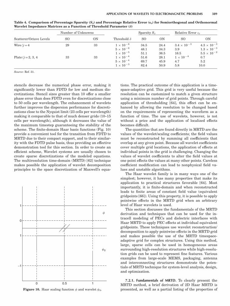
stencils decrease the numerical phase error, making itsignificantly lower than FDTD for low and medium dis-cretizations. Stencil sizes greater than 10 offer a smallerphase error than does FDTD even for discretizations closeto 50 cells per wavelength. The enhancement of waveletsfurther improves the dispersion performance for discreti-zations close to the Nyquist limit (23 cells per wavelength)making it comparable to that of much denser grids (10–15cells per wavelength), although it decreases the value ofthe maximum timestep guaranteeing the stability of thescheme. The finite-domain Haar basis functions (Fig. 10)provide a convenient tool for the transition from FDTD toMRTD due to their compact support, and to their similar-ity with the FDTD pulse basis, thus providing an effectivedemonstration tool for this section. In order to create anefficient scheme, Wavelet systems are usually chosen tocreate sparse discretizations of the modeled equations.The multiresolution time-domain (MRTD) [62] techniquemakes possible the application of wavelet decompositionprinciples to the space discretization of Maxwell’s equa-

tions. The practical outcome of this application is a time-space-adaptive grid. This grid is very useful because theresolution can be customized to match a given structureusing a minimum number of grid points. Through carefulapplication of thresholding [64], this effect can be en-hanced by allowing the resolution to be changed basedon the requirements of representing the waveform as afunction of time. The use of wavelets, however, is notwithout a price and the application of localized effectsbecomes difficult.

The quantities that are found directly in MRTD are thevalues of the wavelet/scaling coefficients; the field valuesmust be reconstructed by summing all coefficients thatoverlap at any given point. Because all wavelet coefficientscover multiple grid locations, the application of effects atindividual points in the grid is challenging. Changing thevalues of wavelet coefficients to alter the field values atone point effects the values at many other points. Carelesscoefficient modification can lead to nonphysical field va-lues and unstable algorithms.

The Haar wavelet family is in many ways one of thesimplest; however, it has many properties that make itsapplication to practical structures favorable [64]. Mostimportantly, it is finite-domain and when reconstructedleads to finite areas of constant field value (equivalentgridpoints [66]). Using this property, it is possible to applypointwise effects in the MRTD grid when an arbitrarylevel of Haar wavelets is used.

This section discusses the fundamentals of the MRTDderivation and techniques that can be used for the in-tracell modeling of PECs and dielectric interfaces withHaar MRTD to apply PEC effects at individual equivalentgridpoints. These techniques use wavelet reconstruction/decomposition to apply pointwise effects in the MRTD gridand makes possible the use of the MRTD timespace-adaptive grid for complex structures. Using this method,large, sparse cells can be used in homogeneous areassurrounding high-resolution structures while high-resolu-tion grids can be used to represent fine features. Variousexamples from large-scale MEMS, packaging, antennaand interconnecting structures demonstrate the poten-tials of MRTD technique for system-level analysis, design,and optimization.

7.2.1. Fundamentals of MRTD. To clearly present theMRTD method, a brief derivation of 2D Haar MRTD ispresented, as well as a partial listing of the properties of

Table 4. Comparison of Percentage Sparsity (Sd) and Percentage Relative Error (ed) for Semiorthogonal and OrthonormalWavelet Impedance Matrices as a Function of Threshold Parameter (d)

Number of Unknowns Sparsity Sd Relative Error ed

Scatterer/Octave Levels SO ON Threshold d SO ON SO ON

Wire / j¼4 29 33 1 � 10� 6 34.5 24.4 3.4 � 10� 3 4.3 � 10� 3

5 � 10� 6 48.1 34.3 3.9 1.3 � 10� 3

1 � 10� 5 51.1 36.5 16.5 5.5 � 10� 2

Plate / j¼2, 3, 4 33 33 1 � 10� 4 51.6 28.1 1 � 10� 4 0.75 � 10� 4 69.7 45.9 4.7 5.21 � 10� 3 82.4 50.9 5.8 10.0

Source: Ref. 31.

1

0

1

−1

0 0.5 1

�

�0

Figure 10. Haar scaling function f and wavelet c0.


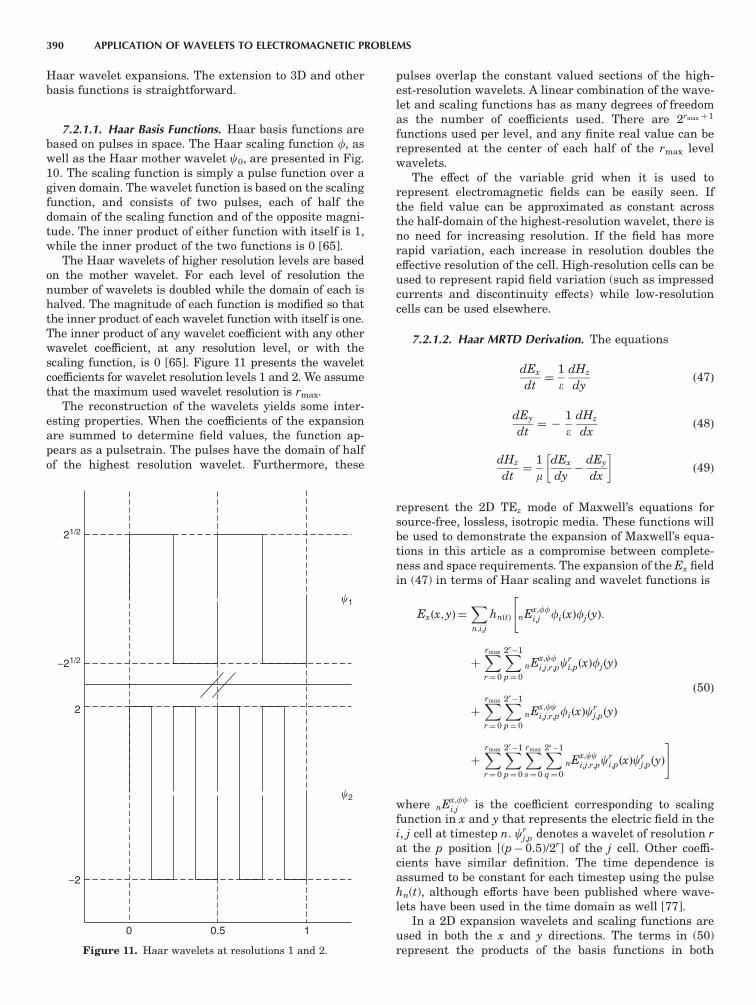
Haar wavelet expansions. The extension to 3D and otherbasis functions is straightforward.

7.2.1.1. Haar Basis Functions. Haar basis functions arebased on pulses in space. The Haar scaling function f, aswell as the Haar mother wavelet c0, are presented in Fig.10. The scaling function is simply a pulse function over agiven domain. The wavelet function is based on the scalingfunction, and consists of two pulses, each of half thedomain of the scaling function and of the opposite magni-tude. The inner product of either function with itself is 1,while the inner product of the two functions is 0 [65].

The Haar wavelets of higher resolution levels are basedon the mother wavelet. For each level of resolution thenumber of wavelets is doubled while the domain of each ishalved. The magnitude of each function is modified so thatthe inner product of each wavelet function with itself is one.The inner product of any wavelet coefficient with any otherwavelet coefficient, at any resolution level, or with thescaling function, is 0 [65]. Figure 11 presents the waveletcoefficients for wavelet resolution levels 1 and 2. We assumethat the maximum used wavelet resolution is rmax.

The reconstruction of the wavelets yields some inter-esting properties. When the coefficients of the expansionare summed to determine field values, the function ap-pears as a pulsetrain. The pulses have the domain of halfof the highest resolution wavelet. Furthermore, these

pulses overlap the constant valued sections of the high-est-resolution wavelets. A linear combination of the wave-let and scaling functions has as many degrees of freedomas the number of coefficients used. There are 2rmax þ 1

functions used per level, and any finite real value can berepresented at the center of each half of the rmax levelwavelets.

The effect of the variable grid when it is used torepresent electromagnetic fields can be easily seen. Ifthe field value can be approximated as constant acrossthe half-domain of the highest-resolution wavelet, there isno need for increasing resolution. If the field has morerapid variation, each increase in resolution doubles theeffective resolution of the cell. High-resolution cells can beused to represent rapid field variation (such as impressedcurrents and discontinuity effects) while low-resolutioncells can be used elsewhere.

7.2.1.2. Haar MRTD Derivation. The equations

dEx

dt¼

1

edHz

dyð47Þ

dEy

dt¼ �

1

edHz

dxð48Þ

dHz

dt¼

1

mdEx

dy�

dEy

dx

� �ð49Þ

represent the 2D TEz mode of Maxwell’s equations forsource-free, lossless, isotropic media. These functions willbe used to demonstrate the expansion of Maxwell’s equa-tions in this article as a compromise between complete-ness and space requirements. The expansion of the Ex fieldin (47) in terms of Haar scaling and wavelet functions is

Exðx; yÞ¼X

n;i;j

hnðtÞ

"

nEx;ffi;j fiðxÞfjðyÞ:

þXrmax

r¼ 0

X2r�1

p¼ 0

nEx;cfi;j;r;pc

ri;pðxÞfjðyÞ

þXrmax

r¼ 0

X2r�1

p¼ 0

nEx;fci;j;r;pfiðxÞc

rj;pðyÞ

þXrmax

r¼ 0

X2r�1

p¼ 0

Xrmax

s¼ 0

X2s�1

q¼0

nEx;cci;j;r;pc

ri;pðxÞc

rj;pðyÞ

#

ð50Þ

where nEx;ffi;j is the coefficient corresponding to scaling

function in x and y that represents the electric field in thei, j cell at timestep n. cr

j;p denotes a wavelet of resolution rat the p position [(p� 0.5)/2r] of the j cell. Other coeffi-cients have similar definition. The time dependence isassumed to be constant for each timestep using the pulsehn(t), although efforts have been published where wave-lets have been used in the time domain as well [77].

In a 2D expansion wavelets and scaling functions areused in both the x and y directions. The terms in (50)represent the products of the basis functions in both

−21/2

−2

0

�1

�2

0.5 1

2

21/2

Figure 11. Haar wavelets at resolutions 1 and 2.


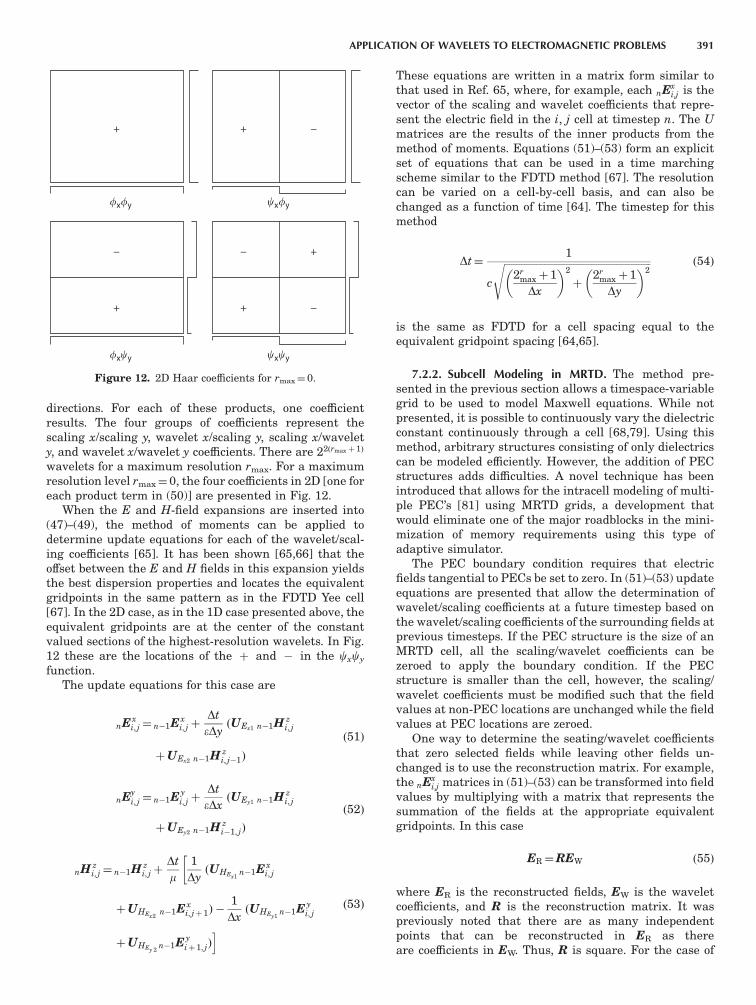
directions. For each of these products, one coefficientresults. The four groups of coefficients represent thescaling x/scaling y, wavelet x/scaling y, scaling x/wavelety, and wavelet x/wavelet y coefficients. There are 22ðrmax þ 1Þ

wavelets for a maximum resolution rmax. For a maximumresolution level rmax¼ 0, the four coefficients in 2D [one foreach product term in (50)] are presented in Fig. 12.

When the E and H-field expansions are inserted into(47)–(49), the method of moments can be applied todetermine update equations for each of the wavelet/scal-ing coefficients [65]. It has been shown [65,66] that theoffset between the E and H fields in this expansion yieldsthe best dispersion properties and locates the equivalentgridpoints in the same pattern as in the FDTD Yee cell[67]. In the 2D case, as in the 1D case presented above, theequivalent gridpoints are at the center of the constantvalued sections of the highest-resolution wavelets. In Fig.12 these are the locations of the þ and � in the cxcy

function.The update equations for this case are

nE xi; j¼ n�1E x

i; jþDt

eDyðUEx1 n�1H z

i; j

þUEx2 n�1H zi; j�1Þ

ð51Þ

nEyi; j¼ n�1E y

i; jþDt

eDxðUEy1 n�1H z

i; j

þUEy2 n�1H zi�1; jÞ

ð52Þ

nH zi; j¼ n�1H z

i; jþDt

m1

DyðUHEx1

n�1E xi; j

�

þUHEx2n�1E x

i; jþ 1Þ �1

DxðUHEy1

n�1E yi; j

þUHEy 2n�1E y

iþ1; jÞ

i

ð53Þ

These equations are written in a matrix form similar tothat used in Ref. 65, where, for example, each nEx

i;j is thevector of the scaling and wavelet coefficients that repre-sent the electric field in the i, j cell at timestep n. The Umatrices are the results of the inner products from themethod of moments. Equations (51)–(53) form an explicitset of equations that can be used in a time marchingscheme similar to the FDTD method [67]. The resolutioncan be varied on a cell-by-cell basis, and can also bechanged as a function of time [64]. The timestep for thismethod

Dt¼1

c

ffiffiffiffiffiffiffiffiffiffiffiffiffiffiffiffiffiffiffiffiffiffiffiffiffiffiffiffiffiffiffiffiffiffiffiffiffiffiffiffiffiffiffiffiffiffiffiffiffiffiffiffiffiffiffiffiffiffiffi2r

maxþ 1

Dx

� �2

þ2r

maxþ1

Dy

� �2s ð54Þ

is the same as FDTD for a cell spacing equal to theequivalent gridpoint spacing [64,65].

7.2.2. Subcell Modeling in MRTD. The method pre-sented in the previous section allows a timespace-variablegrid to be used to model Maxwell equations. While notpresented, it is possible to continuously vary the dielectricconstant continuously through a cell [68,79]. Using thismethod, arbitrary structures consisting of only dielectricscan be modeled efficiently. However, the addition of PECstructures adds difficulties. A novel technique has beenintroduced that allows for the intracell modeling of multi-ple PEC’s [81] using MRTD grids, a development thatwould eliminate one of the major roadblocks in the mini-mization of memory requirements using this type ofadaptive simulator.

The PEC boundary condition requires that electricfields tangential to PECs be set to zero. In (51)–(53) updateequations are presented that allow the determination ofwavelet/scaling coefficients at a future timestep based onthe wavelet/scaling coefficients of the surrounding fields atprevious timesteps. If the PEC structure is the size of anMRTD cell, all the scaling/wavelet coefficients can bezeroed to apply the boundary condition. If the PECstructure is smaller than the cell, however, the scaling/wavelet coefficients must be modified such that the fieldvalues at non-PEC locations are unchanged while the fieldvalues at PEC locations are zeroed.

One way to determine the seating/wavelet coefficientsthat zero selected fields while leaving other fields un-changed is to use the reconstruction matrix. For example,the nEx

i;j matrices in (51)–(53) can be transformed into fieldvalues by multiplying with a matrix that represents thesummation of the fields at the appropriate equivalentgridpoints. In this case

ER¼REW ð55Þ

where ER is the reconstructed fields, EW is the waveletcoefficients, and R is the reconstruction matrix. It waspreviously noted that there are as many independentpoints that can be reconstructed in ER as thereare coefficients in EW. Thus, R is square. For the case of

+

�x�y �x�y

�x�y �x�y

+ −

+ + −

− − +

Figure 12. 2D Haar coefficients for rmax¼0.


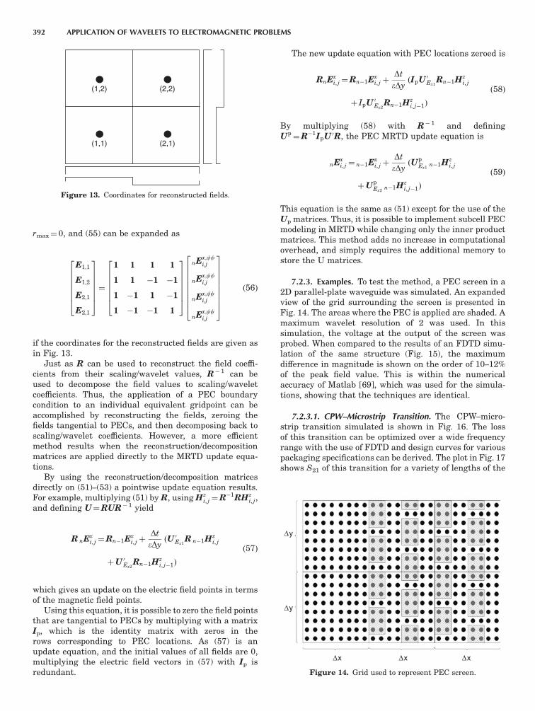
rmax¼ 0, and (55) can be expanded as

E1;1

E1;2

E2;1

E2;1

2

666664

3

777775¼

1 1 1 1

1 1 �1 �1

1 �1 1 �1

1 �1 �1 1

2

666664

3

777775

nEx;ffi;j

nEx;cfi;j

nEx;fci;j

nEx;cci;j

266666664

377777775

ð56Þ

if the coordinates for the reconstructed fields are given asin Fig. 13.

Just as R can be used to reconstruct the field coeffi-cients from their scaling/wavelet values, R�1 can beused to decompose the field values to scaling/waveletcoefficients. Thus, the application of a PEC boundarycondition to an individual equivalent gridpoint can beaccomplished by reconstructing the fields, zeroing thefields tangential to PECs, and then decomposing back toscaling/wavelet coefficients. However, a more efficientmethod results when the reconstruction/decompositionmatrices are applied directly to the MRTD update equa-tions.

By using the reconstruction/decomposition matricesdirectly on (51)–(53) a pointwise update equation results.For example, multiplying (51) by R, using Hz

i; j¼R�1RHzi; j,

and defining U¼RUR�1 yield

R nExi; j¼Rn�1Ex

i; jþDt

eDyðU 0Ex1

R n�1Hzi; j

þU 0Ex2Rn�1Hz

i; j�1Þ

ð57Þ

which gives an update on the electric field points in termsof the magnetic field points.

Using this equation, it is possible to zero the field pointsthat are tangential to PECs by multiplying with a matrixIp, which is the identity matrix with zeros in therows corresponding to PEC locations. As (57) is anupdate equation, and the initial values of all fields are 0,multiplying the electric field vectors in (57) with Ip isredundant.

The new update equation with PEC locations zeroed is

RnExi; j¼Rn�1Ex

i; jþDt

eDyðIpU 0Ex1

Rn�1Hzi; j

þ IpU 0Ex2Rn�1Hz

i; j�1Þ

ð58Þ

By multiplying (58) with R�1 and definingUp¼R�1IpU 0R, the PEC MRTD update equation is

nExi; j¼ n�1Ex

i; jþDt

eDyðUp

Ex1n�1Hz

i; j

þUpEx2

n�1Hzi; j�1Þ

ð59Þ

This equation is the same as (51) except for the use of theUp matrices. Thus, it is possible to implement subcell PECmodeling in MRTD while changing only the inner productmatrices. This method adds no increase in computationaloverhead, and simply requires the additional memory tostore the U matrices.

7.2.3. Examples. To test the method, a PEC screen in a2D parallel-plate waveguide was simulated. An expandedview of the grid surrounding the screen is presented inFig. 14. The areas where the PEC is applied are shaded. Amaximum wavelet resolution of 2 was used. In thissimulation, the voltage at the output of the screen wasprobed. When compared to the results of an FDTD simu-lation of the same structure (Fig. 15), the maximumdifference in magnitude is shown on the order of 10–12%of the peak field value. This is within the numericalaccuracy of Matlab [69], which was used for the simula-tions, showing that the techniques are identical.

7.2.3.1. CPW–Microstrip Transition. The CPW–micro-strip transition simulated is shown in Fig. 16. The lossof this transition can be optimized over a wide frequencyrange with the use of FDTD and design curves for variouspackaging specifications can be derived. The plot in Fig. 17shows S21 of this transition for a variety of lengths of the

(1,2) (2,2)

(1,1) (2,1)

Figure 13. Coordinates for reconstructed fields.

∆x

∆y

∆y

∆x ∆x

Figure 14. Grid used to represent PEC screen.


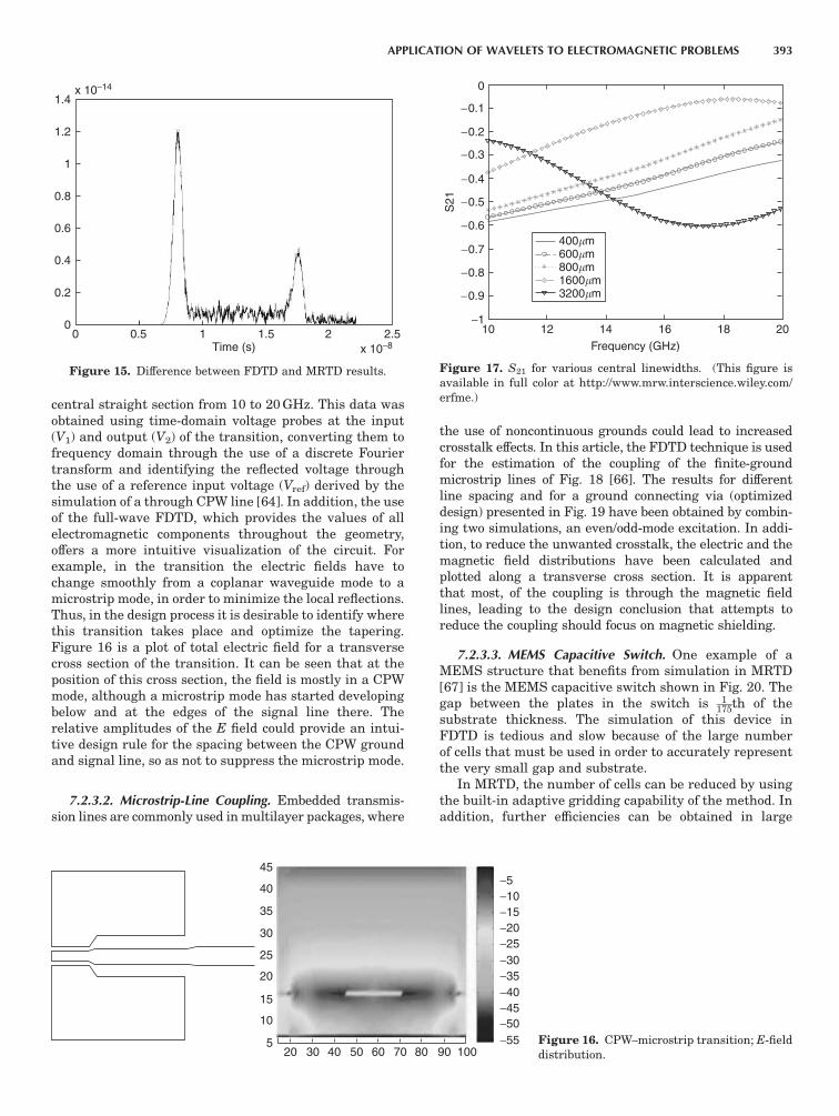
central straight section from 10 to 20 GHz. This data wasobtained using time-domain voltage probes at the input(V1) and output (V2) of the transition, converting them tofrequency domain through the use of a discrete Fouriertransform and identifying the reflected voltage throughthe use of a reference input voltage (Vref) derived by thesimulation of a through CPW line [64]. In addition, the useof the full-wave FDTD, which provides the values of allelectromagnetic components throughout the geometry,offers a more intuitive visualization of the circuit. Forexample, in the transition the electric fields have tochange smoothly from a coplanar waveguide mode to amicrostrip mode, in order to minimize the local reflections.Thus, in the design process it is desirable to identify wherethis transition takes place and optimize the tapering.Figure 16 is a plot of total electric field for a transversecross section of the transition. It can be seen that at theposition of this cross section, the field is mostly in a CPWmode, although a microstrip mode has started developingbelow and at the edges of the signal line there. Therelative amplitudes of the E field could provide an intui-tive design rule for the spacing between the CPW groundand signal line, so as not to suppress the microstrip mode.

7.2.3.2. Microstrip-Line Coupling. Embedded transmis-sion lines are commonly used in multilayer packages, where

the use of noncontinuous grounds could lead to increasedcrosstalk effects. In this article, the FDTD technique is usedfor the estimation of the coupling of the finite-groundmicrostrip lines of Fig. 18 [66]. The results for differentline spacing and for a ground connecting via (optimizeddesign) presented in Fig. 19 have been obtained by combin-ing two simulations, an even/odd-mode excitation. In addi-tion, to reduce the unwanted crosstalk, the electric and themagnetic field distributions have been calculated andplotted along a transverse cross section. It is apparentthat most, of the coupling is through the magnetic fieldlines, leading to the design conclusion that attempts toreduce the coupling should focus on magnetic shielding.

7.2.3.3. MEMS Capacitive Switch. One example of aMEMS structure that benefits from simulation in MRTD[67] is the MEMS capacitive switch shown in Fig. 20. Thegap between the plates in the switch is 1

175th of thesubstrate thickness. The simulation of this device inFDTD is tedious and slow because of the large numberof cells that must be used in order to accurately representthe very small gap and substrate.

In MRTD, the number of cells can be reduced by usingthe built-in adaptive gridding capability of the method. Inaddition, further efficiencies can be obtained in large

1.4

1.2

1

0.8

0.6

0.4

0.2

02.5

x 10−8

x 10−14

21.51Time (s)

0.50

Figure 15. Difference between FDTD and MRTD results.

−5−10−15−20−25−30−35−40−45−50−555

20 30 40 50 60 70 80 90 100

10

15

20

25

30

35

40

45

Figure 16. CPW–microstrip transition; E-fielddistribution.

S21

−0.9

−110 12 14 16

Frequency (GHz)18 20

−0.8

−0.7

−0.6

−0.5

−0.4

−0.3

−0.2

−0.1

0

400�m600�m800�m1600�m3200�m

Figure 17. S21 for various central linewidths. (This figure isavailable in full color at http://www.mrw.interscience.wiley.com/erfme.)


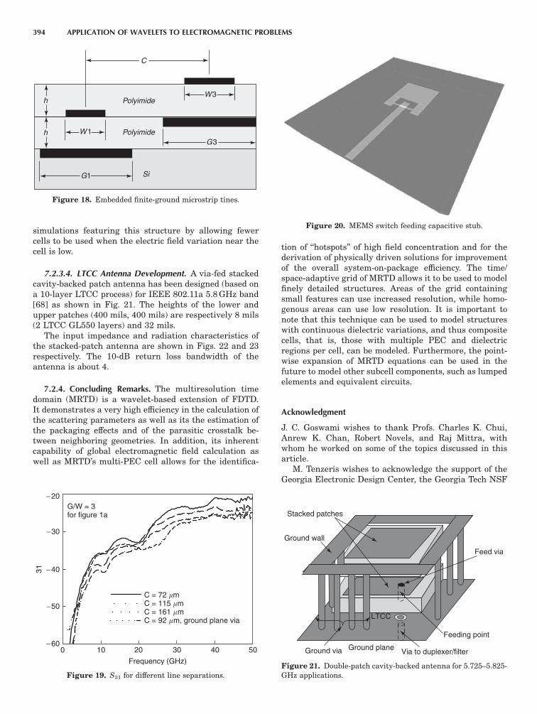
simulations featuring this structure by allowing fewercells to be used when the electric field variation near thecell is low.

7.2.3.4. LTCC Antenna Development. A via-fed stackedcavity-backed patch antenna has been designed (based ona 10-layer LTCC process) for IEEE 802.11a 5.8 GHz band[68] as shown in Fig. 21. The heights of the lower andupper patches (400 mils, 400 mils) are respectively 8 mils(2 LTCC GL550 layers) and 32 mils.

The input impedance and radiation characteristics ofthe stacked-patch antenna are shown in Figs. 22 and 23respectively. The 10-dB return loss bandwidth of theantenna is about 4.

7.2.4. Concluding Remarks. The multiresolution timedomain (MRTD) is a wavelet-based extension of FDTD.It demonstrates a very high efficiency in the calculation ofthe scattering parameters as well as its the estimation ofthe packaging effects and of the parasitic crosstalk be-tween neighboring geometries. In addition, its inherentcapability of global electromagnetic field calculation aswell as MRTD’s multi-PEC cell allows for the identifica-

tion of ‘‘hotspots’’ of high field concentration and for thederivation of physically driven solutions for improvementof the overall system-on-package efficiency. The time/space-adaptive grid of MRTD allows it to be used to modelfinely detailed structures. Areas of the grid containingsmall features can use increased resolution, while homo-genous areas can use low resolution. It is important tonote that this technique can be used to model structureswith continuous dielectric variations, and thus compositecells, that is, those with multiple PEC and dielectricregions per cell, can be modeled. Furthermore, the point-wise expansion of MRTD equations can be used in thefuture to model other subcell components, such as lumpedelements and equivalent circuits.

Acknowledgment

J. C. Goswami wishes to thank Profs. Charles K. Chui,Anrew K. Chan, Robert Novels, and Raj Mittra, withwhom he worked on some of the topics discussed in thisarticle.

M. Tenzeris wishes to acknowledge the support of theGeorgia Electronic Design Center, the Georgia Tech NSF

C

h Polyimide

Polyimide

SiG1

G3W1

W3

h

Figure 18. Embedded finite-ground microstrip tines.

− 20

−30

−40

−50

−600 10 20

Frequency (GHz)

30 40 50

31

G/W = 3for figure 1a

C = 72 �mC = 115 �mC = 161 �mC = 92 �m, ground plane via

Figure 19. S31 for different line separations.

Ground via

Ground wall

Stacked patches

Ground plane

LTCC

Via to duplexer/filter

Feeding point

Feed via

Figure 21. Double-patch cavity-backed antenna for 5.725–5.825-GHz applications.

Figure 20. MEMS switch feeding capacitive stub.


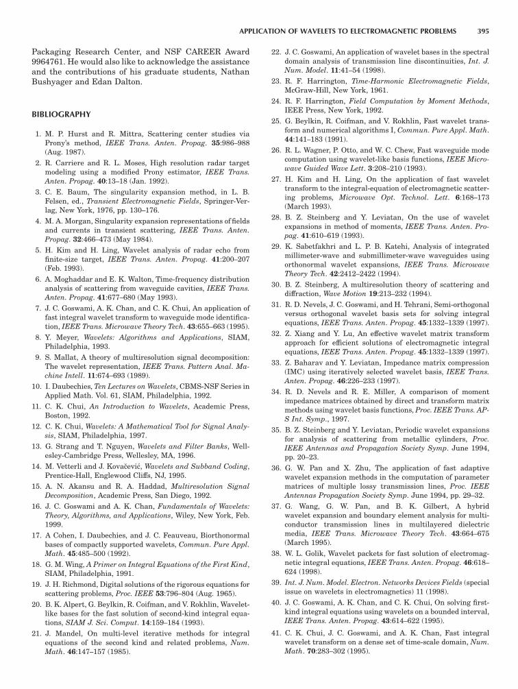
Packaging Research Center, and NSF CAREER Award9964761. He would also like to acknowledge the assistanceand the contributions of his graduate students, NathanBushyager and Edan Dalton.

BIBLIOGRAPHY

1. M. P. Hurst and R. Mittra, Scattering center studies viaProny’s method, IEEE Trans. Anten. Propag. 35:986–988(Aug. 1987).

2. R. Carriere and R. L. Moses, High resolution radar targetmodeling using a modified Prony estimator, IEEE Trans.

Anten. Propag. 40:13–18 (Jan. 1992).

3. C. E. Baum, The singularity expansion method, in L. B.Felsen, ed., Transient Electromagnetic Fields, Springer-Ver-lag, New York, 1976, pp. 130–176.

4. M. A. Morgan, Singularity expansion representations of fieldsand currents in transient scattering, IEEE Trans. Anten.

Propag. 32:466–473 (May 1984).

5. H. Kim and H. Ling, Wavelet analysis of radar echo fromfinite-size target, IEEE Trans. Anten. Propag. 41:200–207(Feb. 1993).

6. A. Moghaddar and E. K. Walton, Time-frequency distributionanalysis of scattering from waveguide cavities, IEEE Trans.Anten. Propag. 41:677–680 (May 1993).

7. J. C. Goswami, A. K. Chan, and C. K. Chui, An application offast integral wavelet transform to waveguide mode identifica-tion, IEEE Trans. Microwave Theory Tech. 43:655–663 (1995).

8. Y. Meyer, Wavelets: Algorithms and Applications, SIAM,Philadelphia, 1993.

9. S. Mallat, A theory of multiresolution signal decomposition:The wavelet representation, IEEE Trans. Pattern Anal. Ma-

chine Intell. 11:674–693 (1989).

10. I. Daubechies, Ten Lectures on Wavelets, CBMS-NSF Series inApplied Math. Vol. 61, SIAM, Philadelphia, 1992.

11. C. K. Chui, An Introduction to Wavelets, Academic Press,Boston, 1992.

12. C. K. Chui, Wavelets: A Mathematical Tool for Signal Analy-sis, SIAM, Philadelphia, 1997.

13. G. Strang and T. Nguyen, Wavelets and Filter Banks, Well-esley-Cambridge Press, Wellesley, MA, 1996.

14. M. Vetterli and J. Kovacevic, Wavelets and Subband Coding,Prentice-Hall, Englewood Cliffs, NJ, 1995.

15. A. N. Akansu and R. A. Haddad, Multiresolution Signal

Decomposition, Academic Press, San Diego, 1992.

16. J. C. Goswami and A. K. Chan, Fundamentals of Wavelets:

Theory, Algorithms, and Applications, Wiley, New York, Feb.1999.

17. A Cohen, I. Daubechies, and J. C. Feauveau, Biorthonormalbases of compactly supported wavelets, Commun. Pure Appl.

Math. 45:485–500 (1992).

18. G. M. Wing, A Primer on Integral Equations of the First Kind,SIAM, Philadelphia, 1991.

19. J. H. Richmond, Digital solutions of the rigorous equations forscattering problems, Proc. IEEE 53:796–804 (Aug. 1965).

20. B. K. Alpert, G. Beylkin, R. Coifman, and V. Rokhlin, Wavelet-like bases for the fast solution of second-kind integral equa-tions, SIAM J. Sci. Comput. 14:159–184 (1993).

21. J. Mandel, On multi-level iterative methods for integralequations of the second kind and related problems, Num.

Math. 46:147–157 (1985).

22. J. C. Goswami, An application of wavelet bases in the spectraldomain analysis of transmission line discontinuities, Int. J.Num. Model. 11:41–54 (1998).

23. R. F. Harrington, Time-Harmonic Electromagnetic Fields,McGraw-Hill, New York, 1961.

24. R. F. Harrington, Field Computation by Moment Methods,IEEE Press, New York, 1992.

25. G. Beylkin, R. Coifman, and V. Rokhlin, Fast wavelet trans-form and numerical algorithms I, Commun. Pure Appl. Math.44:141–183 (1991).

26. R. L. Wagner, P. Otto, and W. C. Chew, Fast waveguide modecomputation using wavelet-like basis functions, IEEE Micro-

wave Guided Wave Lett. 3:208–210 (1993).

27. H. Kim and H. Ling, On the application of fast wavelettransform to the integral-equation of electromagnetic scatter-ing problems, Microwave Opt. Technol. Lett. 6:168–173(March 1993).

28. B. Z. Steinberg and Y. Leviatan, On the use of waveletexpansions in method of moments, IEEE Trans. Anten. Pro-

pag. 41:610–619 (1993).

29. K. Sabetfakhri and L. P. B. Katehi, Analysis of integratedmillimeter-wave and submillimeter-wave waveguides usingorthonormal wavelet expansions, IEEE Trans. Microwave

Theory Tech. 42:2412–2422 (1994).

30. B. Z. Steinberg, A multiresolution theory of scattering anddiffraction, Wave Motion 19:213–232 (1994).

31. R. D. Nevels, J. C. Goswami, and H. Tehrani, Semi-orthogonalversus orthogonal wavelet basis sets for solving integralequations, IEEE Trans. Anten. Propag. 45:1332–1339 (1997).

32. Z. Xiang and Y. Lu, An effective wavelet matrix transformapproach for efficient solutions of electromagnetic integralequations, IEEE Trans. Anten. Propag. 45:1332–1339 (1997).

33. Z. Baharav and Y. Leviatan, Impedance matrix compression(IMC) using iteratively selected wavelet basis, IEEE Trans.Anten. Propag. 46:226–233 (1997).

34. R. D. Nevels and R. E. Miller, A comparison of momentimpedance matrices obtained by direct and transform matrixmethods using wavelet basis functions, Proc. IEEE Trans. AP-S Int. Symp., 1997.

35. B. Z. Steinberg and Y. Leviatan, Periodic wavelet expansionsfor analysis of scattering from metallic cylinders, Proc.

IEEE Antennas and Propagation Society Symp. June 1994,pp. 20–23.

36. G. W. Pan and X. Zhu, The application of fast adaptivewavelet expansion methods in the computation of parametermatrices of multiple lossy transmission lines, Proc. IEEEAntennas Propagation Society Symp. June 1994, pp. 29–32.

37. G. Wang, G. W. Pan, and B. K. Gilbert, A hybridwavelet expansion and boundary element analysis for multi-conductor transmission lines in multilayered dielectricmedia, IEEE Trans. Microwave Theory Tech. 43:664–675(March 1995).

38. W. L. Golik, Wavelet packets for fast solution of electromag-netic integral equations, IEEE Trans. Anten. Propag. 46:618–624 (1998).

39. Int. J. Num. Model. Electron. Networks Devices Fields (specialissue on wavelets in electromagnetics) 11 (1998).

40. J. C. Goswami, A. K. Chan, and C. K. Chui, On solving first-kind integral equations using wavelets on a bounded interval,IEEE Trans. Anten. Propag. 43:614–622 (1995).

41. C. K. Chui, J. C. Goswami, and A. K. Chan, Fast integralwavelet transform on a dense set of time-scale domain, Num.

Math. 70:283–302 (1995).


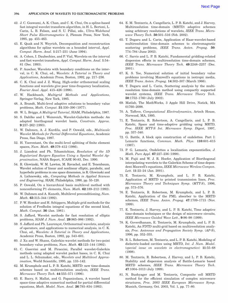
42. J. C. Goswami, A. K. Chan, and C. K. Chui, On a spline-basedfast integral wavelet transform algorithm, in H. L. Bertoni, L.Carin, L. B. Felsen, and S. U. Pillai, eds., Ultra-Wideband

Short Pulse Electromagnetics 2, Plenum Press, New York,1995, pp. 455–463.

43. E. Quak and N. Weyrich, Decomposition and reconstructionalgorithms for spline wavelets on a bounded interval, Appl.

Comput. Harm. Anal. 1:217–231 (June 1994).

44. A. Cohen, I. Daubechies, and P. Vial, Wavelets on the intervaland fast wavelet transform, Appl. Comput. Harm. Anal. 1:54–81 (Dec. 1993).

45. P. Auscher, Wavelets with boundary conditions on the inter-val, in C. K. Chui, ed., Wavelets: A Tutorial in Theory and

Applications, Academic Press, Boston, 1992, pp. 217–236.

46. C. K. Chui and J. Z. Wang, High-order orthonormal scalingfunctions and wavelets give poor time-frequency localization,Fourier Anal. Appl. 415–426 (1996).

47. W. Hackbusch, Multigrid Methods and Applications,Springer-Verlag, New York, 1985.

48. A. Brandt, Multi-level adaptive solutions to boundary valueproblems, Math. Comput. 31:330–390 (1977).

49. W. L. Briggs, A Multigrid Tutorial, SIAM, Philadelphia, 1987.

50. S. Dahlke and I. Weinreich, Wavelet-Galerkin methods: Anadapted biorthogonal wavelet basis, Constrain. Approx.9:237–262 (1993).

51. W. Dahmen, A. J. Kurdila, and P. Oswald, eds., Multiscale

Wavelet Methods for Partial Differential Equations, AcademicPress, San Diego, 1997.

52. H. Yserentant, On the multi-level splitting of finite elementspaces, Num. Math. 49:379–412 (1986).

53. J. Liandrat and Ph. Tchamitchian, Resolution of the 1D

Regularized Burgers Equation Using a Spatial Wavelet Ap-

proximation, NASA Report, ICASE 90-83, Dec. 1990.

54. R. Glowinski, W. M. Lawton, M. Ravachol, and E. Tenenbaum,Wavelet solution of linear and nonlinear elliptic, parabolic, andhyperbolic problems in one space dimension, in R. Glowinski andA. Lichnewsky, eds., Computing Methods in Applied Sciences

and Engineering, SIAM, Philadelphia, 1990, pp. 55–120.

55. P. Oswald, On a hierarchical basis multilevel method withnonconforming P1 elements, Num. Math. 62:189–212 (1992).

56. W. Dahmen and A. Kunoth, Multilevel preconditioning, Num.

Math. 63:315–344 (1992).

57. P. W. Hemker and H. Schippers, Multiple grid methods for thesolution of Fredholm integral equations of the second kind,Math. Comput. 36 (Jan. 1981).

58. S. Jaffard, Wavelet methods for fast resolution of ellipticproblems, SIAM J. Num. Anal. 29:965–986 (1992).

59. S. Jaffard and Ph. Laurenc,ot, Orthonormal wavelets, analysisof operators, and applications to numerical analysis, in C. K.Chui, ed., Wavelets: A Tutorial in Theory and Applications,Academic Press, Boston, 1992, pp. 543–601.

60. J. Xu and W. Shann, Galerkin-wavelet methods for two-pointboundary value problems, Num. Math. 63:123–144 (1992).

61. C. Guerrini and M. Piraccini, Parallel wavelet-Galerkinmethods using adapted wavelet packet bases, in C. K. Chuiand L. L. Schumaker, eds., Wavelets and Multilevel Approx-

imation, World Scientific, 1995, pp. 133–142.

62. M. Krumpholz and L. P. B. Katehi, MRTD: new time-domainschemes based on multiresolution analysis, IEEE Trans.

Microwave Theory Tech. 44:555–571 (1996).

63. E. Bacry, S. Mallat, and G. Papanicolaou, A wavelet basedspace-time adaptive numerical method for partial differentialequations, Math. Model. Num. Anal. 26:793–834 (1992).

64. E. M. Tentzeris, A. Cangellaris, L. P. B. Katehi, and J. Harvey,Multiresolution time-domain (MRTD) adaptive schemesusing arbitrary resolutions of wavelets, IEEE Trans. Micro-

wave Theory Tech. 50:501–516 (Feb. 2002).

65. T. Dogaru and L. Carin, Application of Haar-wavelet-basedmultiresolution time-domain schemes to electromagneticscattering problems, IEEE Trans. Anten. Propag. 50:774–784 (June 2002).

66. C. Sarris and L. P. B. Katehi, Fundamental gridding-relateddispersion effects in multiresolution time-domain schemes,IEEE Trans. Microwave Theory Tech. 49:2248–2257 (Dec.2001).

67. K. S. Yee, Numerical solution of initial boundary valueproblems involving Maxwell’s equations in isotropic media,IEEE Trans. Anten. Propag. 14:302–307 (March 1966).

68. T. Dogaru and L. Carin, Scattering analysis by the multi-resolution time-domain method using compactly supportedwavelet systems, IEEE Trans. Microwave Theory Tech.50:1752–1760 (July 2002).

69. Matlab, The MathWorks, 3 Apple Hill Drive, Natick, MA01760–2098.

70. A. Taflove, Computational Electrodynamics, Artech House,Norwood, MA, 1995.

71. E. Tentzeris, R. Robertson, A. Cangellaris, and L. P. B.Katehi, Space and time-adaptive gridding using MRTD,Proc. IEEE MTT-S Int. Microwave Symp. Digest, 1997,pp. 337–340.

72. G. Battle, A block spin construction of ondelettes. Part I:Lemarie functions, Commun. Math. Phys. 110:601–615(1987).

73. P. G. Lemarie, Ondelettes a localization exponentielles, J.

Math. Pure Appl. 67:227–236 (1998).

74. M. Fujii and W. J. R. Hoefer, Application of Biorthogonalinterpolating wavelets to the Galerkin Scheme of time-depen-dent Maxwell’s equations, IEEE Microwave Wireless Compon.

Lett. 11:22–24 (Jan. 2001).

75. E. Tentzeris, M. Krumpholz, and L. P. B. Katehi,Application of MRTD to printed transmission lines, Proc.

Microwave Theory and Techniques Symp. (MTT-S), 1996,pp. 573–576.

76. E. Tentzeris, R. Robertson, M. Krumpholz, and L. P. B.Katehi, Application of the PML absorber to the MRTDschemes, IEEE Trans. Anten. Propag. 47:1709–1715 (Nov.1999).

77. E. Tentzeris, J. Harvey, and L. P. B. Katehi, Time adaptivetime-domain techniques or the design of microwave circuits,IEEE Microwave Guided Wave Lett., 9:96–98 (1999).

78. K. Goverdhanam, E. Tentzeris, M. Krumpholz, and L. P. B.Katehi, An FDTD multi-grid based on multiresolution analy-sis, Proc. Antennas and Propagation Society Symp. (AP-S),1996, pp. 352–355.

79. R. L. Robertson, M. Tentzeris, and L. P. B. Katehi, Modeling ofdielectric-loaded cavities using MRTD, Int. J. Num. Model.(special issue on wavelets in electromagnetics) 11:55–68(1998).

80. M. Tentzeris, R. Robertson, J. Harvey, and L. P. B. Katehi,Stability and dispersion analysis of Battle-Lemarie basedMRTD schemes, IEEE Trans. Microwave Theory Tech.47:1004–1013 (July 1999).

81. N. Bushyager and M. Tentzeris, Composite cell MRTDmethod for the efficient simulation of complex microwavestructures, Proc. 2003 IEEE European Microwave Symp.Munich, Germany, Oct. 2003, Vol. 1, pp. 77–80.


Next Page

Documents

APERTURE ANTENNAS - Eefocusdata.eefocus.com/myspace/0/942/bbs/1174163529/a7c74d4.pdf · antenna system for portable equipment—II; ... a principle by which the actual sources on