AP Stats Chapter 9 Notes - Miami-Dade County Public Schoolsteachers.dadeschools.net/sdaniel/AP Stats Chapter 9 Notes.pdfChapter 9 3 State the Hypothesis & Parameter: p= true proportion

Chapter 9

1

Section 9.1

Significance Tests: The Basics

Section 9.1Significance Tests: The Basics

After this section, you should be able to…

STATE correct hypotheses for a significance test about a population proportion or mean.

INTERPRET P‐values in context.

INTERPRET a Type I error and a Type II error in context, and give the consequences of each.

DESCRIBE the relationship between the significance level of a test, P(Type II error), and power.

Statistical Inference

Significance Tests‐

• ASSESS the evidence provided by data about some claim concerning a population

• Reject or fail to reject (Yes vs. No)

Confidence Interval ‐

• ESTIMATE a population parameter.

• Give range of possible values

Significance Test

A significance test is a formal procedure for comparing observed data with a claim (also called a hypothesis) whose truth we want to assess.

The claim is a statement about a parameter, like the population proportion p or the population mean µ.

We express the results of a significance test in terms of a probability (p‐value) that measures how well the data and the claim agree.

The Reasoning of Significance Tests

Statistical tests deal with claims about a population. Tests ask if sample data give good evidence against a claim. A test might say, “If we took many random samples and the claim were true, what is the probability we will get a result like this.”

For example: Suppose a basketball player claimed to be an 80% free‐throw shooter. To test this claim, we have him attempt 50 free‐throws. He makes 32 of them. His sample proportion of made shots is 32/50 = 0.64.

What can we conclude about the claim based on this sample data? What is the probability the player is telling the

truth?!?!


We can use software to simulate 400 sets of 50 shots assuming that the player is really an 80% shooter.

Chapter 9

2


The observed statistic is so unlikely if the actual parameter value is p = 0.80 that it gives convincingevidence that the player’s claim is not true.

You can say how strong the evidence against the player’s claim is by giving the probability that he would make as few as 32 out of 50 free throws if he really makes 80% in the long run.

The Reasoning of Significance TestsBased on the evidence, we might conclude the player’s claim is incorrect. In reality, there are two possible explanations for the fact that he made only 64% of his free throws.

1) The player’s claim is correct (p = 0.8), and by horrible luck, a very unlikely outcome occurred.

2) The population proportion is actually less than 0.8, so the sample result is not an unlikely outcome.

An outcome that would rarely happen if a claim were true is good evidence that the claim is not true.

Basic Idea

Stating Hypotheses

The claim tested by a statistical test is called the null hypothesis (H0). The test is designed to assess the strength of the evidence against the null hypothesis. Often the null hypothesis is a statement of “no difference” or that the claim is true.

The claim about the population that we are trying to find evidence for is the alternative hypothesis (Ha).

In the free‐throw shooter example, our hypotheses are

H0 : p = 0.80Ha : p < 0.80

Parameter: p = the long‐run proportion of made free throws.

Stating Hypotheses

In any significance test, the null hypothesis has the formH0 : parameter = value

The alternative hypothesis has one of the formsHa : parameter < value Ha : parameter > valueHa : parameter ≠ value

To determine the correct form of Ha, read the problem carefully.

Stating Hypotheses• The alternative hypothesis is one‐sided if it states that a

parameter is larger than the null hypothesis value or if it states that the parameter is smaller than the null value.

• It is two‐sided if it states that the parameter is different from the null hypothesis value (it could be either larger or smaller). Use Ha : parameter ≠ value for two sided.

• Hypotheses always refer to a population, not to a sample. Be sure to state H0 and Ha in terms of population parameters (p or ).

• It is never correct to write a hypothesis about a sample statistic, such as

State the Hypothesis & Parameter:

A high school junior running for student body president, Sally, claims that 80% of the student body favors her in the school election. Her opponent believes this percentage to be lower, write the appropriate null and alternative hypotheses.

Chapter 9

3

State the Hypothesis & Parameter:

p= true proportion of students that favor Sally for president.

Interpreting P‐Values

• The null hypothesis H0 states the claim that we are seeking evidence against.

• The probability that measures the strength of the evidence against a null hypothesis is called a P‐value.

• The probability, computed assuming H0 is true, that the statistic would take a value as extreme as or more extreme than the one actually observed is called the P‐value of the test.

• The smaller the P‐value, the stronger the evidence against H0 provided by the data.

H0: µ = 0 English Math

Small P‐value

Evidence against

Unlikely to occur if H0 is true

We reject H0

Large P‐value

Not convincing evidence

Could occur if H0 is true

We fail to reject H0

Example: Studying Job SatisfactionDoes the job satisfaction of assembly‐line workers differ when their work is machine‐paced rather than self‐paced? One study chose 18 subjects at random from a company with over 200 workers who assembled electronic devices. Half of the workers were assigned at random to each of two groups. Both groups did similar assembly work, but one group was allowed to pace themselves while the other group used an assembly line that moved at a fixed pace. After two weeks, all the workers took a test of job satisfaction. Then they switched work setups and took the test again after two more weeks. The response variable is the difference in satisfaction scores, self‐paced minus machine‐paced.

a) Describe the parameter of interest in this setting.

b) State appropriate hypotheses for performing a significance test.

Example: Studying Job Satisfactiona) Describe the parameter of interest in this setting.

b) State appropriate hypotheses for performing a significance test.

The parameter of interest is the mean µ of the differences (self‐paced minus machine‐paced) in job satisfaction scores in the population of all assembly‐line workers at this company. (FYI‐Matched pairs!!!)

Because the initial question asked whether job satisfaction differs, the alternative hypothesis is two‐sided; that is, either µ < 0 or µ > 0. For simplicity, we write this as µ ≠ 0. That is,

H0: µ = 0Ha: µ ≠ 0

Example: Studying Job Satisfaction

c) Explain what it means for the null hypothesis to be true in this setting.

For the job satisfaction study, the hypotheses areH0: µ = 0Ha: µ ≠ 0

d) Interpret the given P‐value in context.

Chapter 9

4


c) Explain what it means for the null hypothesis to be true in this setting.

For the job satisfaction study, the hypotheses areH0: µ = 0Ha: µ ≠ 0

In this setting, the null hypothesis is that there is no mean difference in employee satisfaction scores (self‐paced ‐machine‐paced) for the entire population of assembly‐line workers at the company. If null hypothesis is true, then the workers don’t favor one work environment over the other, on average.


d) Interpret the P-value in context.

The P‐value is the probability of observing a sample result as extreme as (or more extreme) by pure chance given that the null hypothesis is actually true.

Since the test is two‐sided, we have a 23% chance of observing a value that is 17 points or more from the mean, in either direction. An outcome that would occur so often just by chance (almost 1 in every 4 random samples of 18 workers) when the null is true is not convincing evidence against null.

We fail to reject H0: µ = 0.

Conclusion: Statistical Significance

We will make one of two decisions based on the strength of the evidence against the null hypothesis (and in favor of the alternative hypothesis) ‐‐ reject H0 or fail to reject H0.

If our sample result is too unlikely to have happened by chance assuming H0 is true, then we’ll reject H0.

Otherwise, we will fail to reject H0.

A fail‐to‐reject H0 decision in a significance test doesn’t mean that H0 is true. For that reason, you should never “accept H0” or use language implying that you believe H0

is true.

Statistically Significant

• There is no perfect rule for how small a P‐value we should require in order to reject H0 — it’s a matter of judgment and depends on the specific circumstances.

• We can compare the P‐value with a fixed value (typically α = 0.05), called the significance level (alpha α).

• When our p‐value is greater than the chosen α, there is no statistically significance. We “fail to reject” the null.

• When our P‐value is less than the chosen α, we say that the result is statistically significant.

– In that case, we reject the null hypothesis H0 and conclude that there is convincing evidence in favor of the alternative hypothesis Ha.

General conclusion in a significance test :

P‐value small → reject H0 → conclude Ha

P‐value large → fail to reject H0 → cannot conclude Ha

Conclusion with fixed level of significance :

P‐value < α → reject H0 → conclude Ha

P‐value ≥ α → fail to reject H0 → cannot conclude Ha

Example: Better Batteries

a) What conclusion can you make for the significance level α = 0.05?

b) What conclusion can you make for the significance level α = 0.01?

A company has developed a new deluxe AAA battery that is supposed to last longer than its regular AAA battery. However, these new batteries are more expensive to produce, so the company would like to be convinced that they really do last longer. Based on years of experience, the company knows that its regular AAA batteries last for 30 hours of continuous use, on average. The company selects an SRS of 15 new batteries and uses them continuously until they are completely drained. A significance test is performed using the hypotheses

H0 : µ = 30 hours Ha : µ > 30 hours

where µ is the true mean lifetime of the new deluxe AAA batteries. The resulting P‐value is 0.0276.

Chapter 9

5

Example: Better Batteries

a) What conclusion can you make for the significance level α = 0.05?

b) What conclusion can you make at significance level α = 0.01?

Since the P‐value, 0.0276, is less than α = 0.05, the sample result is statistically significant at the 5% level. We have sufficient evidence to reject the null hypothesis and have sufficient evidence to conclude that the company’s deluxe AAA batteries last longer than 30 hours, on average.

Since the P‐value, 0.0276, is greater than α = 0.01, the sample result is not statistically significant at the 1% level. We fail to reject the null hypothesis; therefore, we cannot conclude that the deluxe AAA batteries last longer than 30 hours, on average.

Type I and Type II Errors

Type I error

Reject H0 when H0 is true

Type II error

Fail to reject H0 when H0 is false

Double F = Type II

Type I & II Errors

Type I & II Errors

American Justice System Example:

• Ho: innocent

• Ha: guilty

• Type I error: punish an innocent person

• Type II error: let a not innocent (guilty) person go free

More: http://www.intuitor.com/statistics/T1T2Errors.html

Type I & II Errors

Type I and II Errors

Quality Control Example:

• Ho: the product is acceptable to the customer

• Ha: the product is unacceptable to the customer

• type I error: reject acceptable product and don't ship it.

• type 2 error: ship unacceptable product to the customer

Chapter 9

6

Example: Perfect Potatoes

Describe a Type I and a Type II error in this setting, and explain the consequences of each.

A potato chip producer and its main supplier agree that each shipment of potatoes must meet certain quality standards. If the producer determines that more than 8% of the potatoes in the shipment have “blemishes,” the truck will be sent away to get another load of potatoes from the supplier. Otherwise, the entire truckload will be used to make potato chips. To make the decision, a supervisor will inspect a random sample of potatoes from the shipment. The producer will then perform a significance test using the hypotheses

H0 : p = 0.08Ha : p > 0.08

where p is the actual proportion of potatoes with blemishes in a given truckload.

Example: Perfect Potatoes

Describe a Type I and a Type II error in this setting, and explain the consequences of each.

• A Type I error would occur if the producer concludes that the proportion of potatoes with blemishes is greater than 0.08 when the actual proportion is 0.08 (or less). Consequence: The potato‐chip producer sends the truckload of acceptable potatoes away, which may result in lost revenue for the supplier.

• A Type II error would occur if the producer does not send the truck away when more than 8% of the potatoes in the shipment have blemishes. Consequence: The producer uses the truckload of potatoes to make potato chips. More chips will be made with blemished potatoes, which may upset consumers.

The probability of making a Type 1 error is ALWSYS equal to the significance level ( ).

The probability of making a Type 1 error is 1 ‐ . Beta is the “power” of the test.

Power

• The probability of NOTmaking a Type II error.

• The higher the power, the less likely the mistake is.

Factors that Increase Power• Sample Size

– The larger the sample size, the higher the power.

• Alpha Significance Level– Increasing alpha (from 0.01 to 0.05) increases the power, because a less conservative alpha increases the chance of (correctly) rejecting the null.

• Value of the Alternative Parameter– The greater the difference between the Hypothesized and True Mean the more obvious the result and therefore the greater the power.

More: https://onlinecourses.science.psu.edu/stat414/book/export/html/245

Increase Power, Decrease Type II

Chapter 9

7

Increase Power, Decrease Type II

Blue = PowerRed = Type II error

What’s Worse? Type I or II

• It depends.

• It’s impossible to minimize both error types completely.

More on Type 1 and 2 Errors

Error ProbabilitiesWe can assess the performance of a significance test by looking at the probabilities of

the two types of error. That’s because statistical inference is based on asking, “What would happen if I did this many times?”

For the truckload of potatoes in the previous example, we were testingH0 : p = 0.08Ha : p > 0.08

where p is the actual proportion of potatoes with blemishes. Suppose that the potato‐chip producer decides to carry out this test based on a random sample of 500 potatoes using a 5% significance level (α = 0.05).

Error Probabilities

The shaded area in the right tail is 5%. Sample proportion values to the right of the green line at 0.0999 will cause us to reject H0 even though H0 is true. This will happen in 5% of all possible samples. That is, P(making a Type I error) = 0.05.

Type 2 Errors Investigation WS

www.rossmanchance.com/applets

Select: Improved Batting Averages (Power)

Or direct link:

http://statweb.calpoly.edu/chance/applets/power/power.html

Chapter 9

8

Error ProbabilitiesThe potato‐chip producer wonders whether the significance test of H0 : p = 0.08 versus Ha : p > 0.08 based on a random sample of 500 potatoes has enough power to detect a shipment with, say, 11% blemished potatoes. In this case, a particular Type II error is to fail to reject H0 : p = 0.08 when p = 0.11.

What if p = 0.11?

• Error ProbabilitiesThe potato‐chip producer wonders whether the significance test of H0 : p = 0.08 versus Ha : p

> 0.08 based on a random sample of 500 potatoes has enough power to detect a shipment with, say, 11% blemished potatoes. In this case, a particular Type II error is to fail to reject H0 : p = 0.08 when p = 0.11. Earlier, we decided to reject H0

at α = 0.05 if our sample yielded a sample proportion to the right of the green line.

Since we reject H0 at α= 0.05 if our sample yields a proportion > 0.0999, we’d correctly reject the shipment about 75% of the time.

The power of a test against any alternative is 1 minus the probability of a Type II error for that alternative; that is, power = 1 - β.

Power and Type II Error


Summary

In this section, we learned that…

A significance test assesses the evidence provided by data against a null hypothesis H0 in favor of an alternative hypothesis Ha.

The hypotheses are stated in terms of population parameters. Often, H0 is a statement of no change or no difference. Ha says that a parameter differs from its null hypothesis value in a specific direction (one‐sided alternative) or in either direction (two‐sided alternative).

The reasoning of a significance test is as follows. Suppose that the null hypothesis is true. If we repeated our data production many times, would we often get data as inconsistent with H0 as the data we actually have? If the data are unlikely when H0 is true, they provide evidence against H0 .

The P‐value of a test is the probability, computed supposing H0 to be true, that the statistic will take a value at least as extreme as that actually observed in the direction specified by Ha .


Summary

Small P‐values indicate strong evidence against H0 . To calculate a P‐value, we must know the sampling distribution of the test statistic when H0 is true. There is no universal rule for how small a P‐value in a significance test provides convincing evidence against the null hypothesis.

If the P‐value is smaller than a specified value α (called the significance level), the data are statistically significant at level α. In that case, we can reject H0 . If the P‐value is greater than or equal to α, we fail to reject H0 .

A Type I error occurs if we reject H0 when it is in fact true. A Type II error occurs if we fail to reject H0 when it is actually false. In a fixed level αsignificance test, the probability of a Type I error is the significance level α.

The power of a significance test against a specific alternative is the probability that the test will reject H0 when the alternative is true. Power measures the ability of the test to detect an alternative value of the parameter. For a specific alternative, P(Type II error) = 1 ‐ power.

Section 9.2Tests About a Population Proportion

Section 9.2Tests About a Population Proportion


CHECK conditions for carrying out a test about a population proportion.

CONDUCT a significance test about a population proportion.

CONSTRUCT a confidence interval to draw a conclusion about for a two‐sided test about a population proportion.

Chapter 9

9

Carrying Out a Significance Test

Recall our basketball player who claimed to be an 80% free‐throw shooter. In an SRS of 50 free‐throws, he made 32. His sample proportion of made shots, 32/50 = 0.64, is much lower than what he claimed.

Does it provide convincing evidence against his claim? We use z‐scores and p‐values to evaluate.

Theory: One‐Sample z Test for a Proportion

The z statistic has approximately the standard Normal distribution when H0 is true.

Theory: Test Statistic and P‐valueA significance test uses sample data to measure the strength of evidence against H0.

• The test compares a statistic calculated from sample data with the value of the parameter stated by the null hypothesis.

• Values of the statistic far from the null parameter value in the direction specified by the alternative hypothesis give evidence against H0.

• A test statistic measures how far a sample statistic diverges from what we would expect if the null hypothesis H0 were true.


P Parameters

H Hypothesis

A Assess Conditions

N Name the Test

T Test Statistic (Calculate)

O Obtain P‐value

M Make a decision

S State conclusion


Parameters & Hypothesis

Parameter: p = the actual proportion of free throws the shooter makes in the long run.

Hypothesis:

H0: p = 0.80Ha: p < 0.80


Assess Conditions: Random, Normal & Independent.

RandomWe can view this set of 50 shots as a simple random sample from the population of all possible shots that the player takes.

Normal Assuming H0 is true, p = 0.80. then np = (50)(0.80) = 40 and n (1 ‐ p) = (50)(0.20) = 10 are both at least 10, so the normal condition is met.

Independent In our simulation, the outcome of each shot does is determined by a random number generator, so individual observations are independent.

Chapter 9

10

Carrying Out a Significance TestName the Test, Test Statistic (Calculate) & Obtain P‐value

Name Test: One‐proportion z‐test

Z‐ score: ‐2.83

P‐ value: 0.0023


Name the Test

TINspire: Menu, 6: Statistics, 7: Stats Tests, 5: 1‐Prop z Test


Test Statistic (Calculate) & Obtain P‐value

Carrying Out a Significance TestMake a Decision & State the Conclusion

Make a Decision: P‐value is 0.0023. Since the p‐value is so small we reject the null hypothesis.

State the Conclusion: We have convincing evidence that the basketball player does not make 80% of his free throws.

Example: One Potato, Two Potato

A potato‐chip producer has just received a truckload of potatoes from its main supplier. If the producer determines that more than 8% of the potatoes in the shipment have blemishes, the truck will be sent away to get another load from the supplier. A supervisor selects a random sample of 500 potatoes from the truck. An inspection reveals that 47 of the potatoes have blemishes. Carry out a significance test at the α= 0.10 significance level. What should the producer conclude?


State Parameter & State Hypothesis

α = 0.10 significance level

Parameter: p = actual proportion of potatoes in this shipment with blemishes.

Hypothesis: H0: p = 0.08Ha: p > 0.08

Chapter 9

11


Assess Check ConditionsRandom

Random sample of 500 potatoes Normal

Assuming H0: p = 0.08 is true, the expected numbers of blemished and unblemished potatoes are np0 = 500(0.08) = 40 and n(1 ‐ p0) = 500(0.92) = 460, respectively. Because both of these values are at least 10, we should be safe doing Normal calculations.

Independent Because we are sampling without replacement, we need to check the 10% condition. It seems reasonable to assume that there are at least 10(500) = 5000 potatoes in the shipment.


Name the Test


Test Statistic (Calculate) and Obtain P‐value


Make a Decision and State Conclusion

Make a Decision: Since our P‐value, 0.1251, is greater than the chosen significance level of α = 0.10, so we fail to reject the null hypothesis.

State Conclusion: There is not sufficient evidence to conclude that the shipment contains more than 8% blemished potatoes. The producer will use this truckload of potatoes to make potato chips.

Smoking in High School

According to the Centers for Disease Control and Prevention (CDC) Web site, 50% of high school students have never smoked a cigarette. Taeyeon wonders whether this national result holds true in his large, urban high school. For his AP Statistics class project, Taeyeon surveys an SRS of 150 students from his school. He gets responses from all 150 students, and 90 say that they have never smoked a cigarette. What should Taeyeon conclude? Give appropriate evidence to support your answer.


Perform at test at the α = 0.05 significance level

Parameter: p = actual proportion of students in Taeyeon’sschool who would say they have never smoked cigarettes

Hypothesis:H0: p = 0.50Ha: p ≠ 0.50

Chapter 9

12

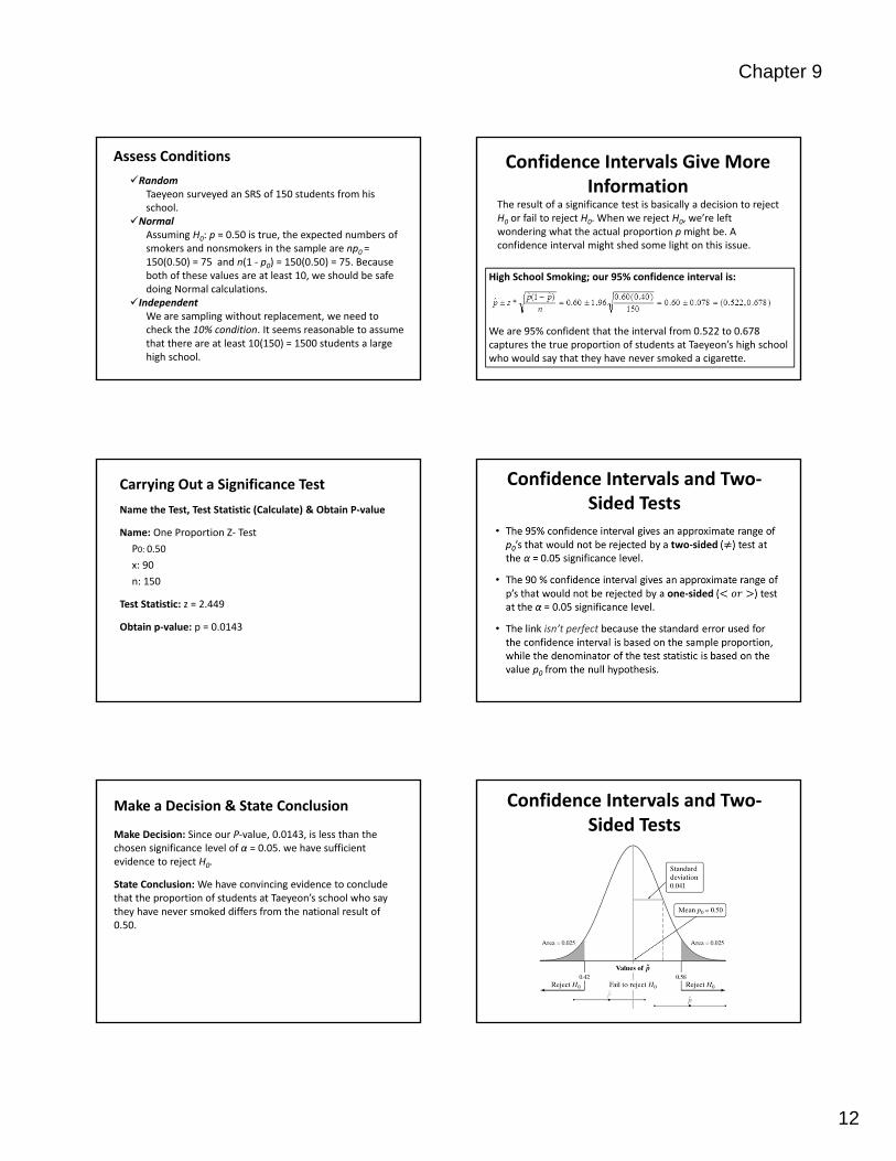
Assess Conditions

Random Taeyeon surveyed an SRS of 150 students from his school.

Normal Assuming H0: p = 0.50 is true, the expected numbers of smokers and nonsmokers in the sample are np0 = 150(0.50) = 75 and n(1 ‐ p0) = 150(0.50) = 75. Because both of these values are at least 10, we should be safe doing Normal calculations.

Independent We are sampling without replacement, we need to check the 10% condition. It seems reasonable to assume that there are at least 10(150) = 1500 students a large high school.


Name the Test, Test Statistic (Calculate) & Obtain P‐value

Name: One Proportion Z‐ Test

P0: 0.50

x: 90

n: 150

Test Statistic: z = 2.449

Obtain p‐value: p = 0.0143

Make a Decision & State Conclusion

Make Decision: Since our P‐value, 0.0143, is less than the chosen significance level of α = 0.05. we have sufficient evidence to reject H0.

State Conclusion: We have convincing evidence to conclude that the proportion of students at Taeyeon’s school who say they have never smoked differs from the national result of 0.50.

Confidence Intervals Give More Information

The result of a significance test is basically a decision to reject H0 or fail to reject H0. When we reject H0, we’re left wondering what the actual proportion p might be. A confidence interval might shed some light on this issue.

High School Smoking; our 95% confidence interval is:

We are 95% confident that the interval from 0.522 to 0.678 captures the true proportion of students at Taeyeon’s high school who would say that they have never smoked a cigarette.

Confidence Intervals and Two‐Sided Tests


Chapter 9

13

One Proportion Z‐Test by Hand

Basketball‐ Carrying Out a Significance TestStep 3a: Calculate Mean & Standard Deviation

If the null hypothesis H0 : p = 0.80 is true, then the player’s sample proportion of made free throws in an SRS of 50 shots would vary according to an approximately Normal sampling distribution with mean

Basketball‐ Carrying Out a Significance TestStep 3b: Calculate Test Statistic

Then, Using Table A, we find that the P‐value is P(z ≤ – 2.83) = 0.0023.


Step 3: CalculationsThe sample proportion of blemished potatoes is

P‐value Using Table A the desired P‐value isP(z ≥ 1.15) = 1 – 0.8749 = 0.1251

High School Smoking

The sample proportion is

P‐value To compute this P‐value, we find the area in one tail and double it. Using Table A or normalcdf(2.45, 100) yields P(z ≥ 2.45) = 0.0071 (the right‐tail area). So the desired P‐value is2(0.0071) = 0.0142.

Section 9.3Tests About a

Population Mean

Chapter 9

14

Section 9.3Tests About a Population Mean


CHECK conditions for carrying out a test about a population mean.

CONDUCT a one‐sample t test about a population mean.

CONSTRUCT a confidence interval to draw a conclusion for a two‐sided test about a population mean.

PERFORM significance tests for paired data.

Introduction

Confidence intervals and significance tests for a population proportion p are based on z‐values from the standard Normal distribution.

Reminder: Inference about a population mean µ uses a t distribution with n ‐ 1 degrees of freedom, except in the rare case when the population standard deviation σ is known.

The One‐Sample t Test

Choose an SRS of size n from a large population that contains an unknown mean µ. To test the hypothesis H0 : µ = µ0, compute the one‐sample t statistic

Find the P‐value by calculating the probability of getting a t statistic this large or larger in the direction specified by the alternative hypothesis Ha in a t‐distribution with df = n ‐ 1

Carrying Out a Significance Test for µ

ABC company claimed to have developed a new AAA battery that lasts longer than its regular AAA batteries. Based on years of experience, the company knows that its regular AAA batteries last for 30 hours of continuous use, on average. An SRS of 15 new batteries lasted an average of 33.9 hours with a standard deviation of 9.8 hours. Do these data give convincing evidence that the new batteries last longer on average?


Parameter: µ = the true mean lifetime of the new deluxe AAA batteries.

Hypothesis:

H0: µ = 30 hours

Ha: µ > 30 hours

Assess ConditionsRandom, Normal, and Independent.

Random: The company tests an SRS of 15 new AAA batteries. Normal: With such a small sample size (n = 15), we need to inspect the data for any departures from Normality.

Independent Since the batteries are being sampled without replacement, we need to check the 10% condition10% Condition: There must be at least 10(15) = 150 new AAA batteries. This seems reasonable to believe.

The boxplot show slight right‐skewness but no outliers. We should be safe performing a t‐test about the population mean lifetime µ.

Chapter 9

15

Name Test, Test statistic (Calculation) and Obtain P‐value

One sample t‐ test

t: 1.5413 df = 14

p‐value: 0.072771

Make a Decision & State Conclusion

Make a Decision: Since the p‐value of 0.072 exceeds our α = 0.05 significance level, we fail to reject the null hypothesis and

Make a Conclusion: we can’t conclude that the company’s new AAA batteries last longer than 30 hours, on average.

Details: Normal Condition

• The Normal condition for means is either population distribution is Normal or sample size is large (n ≥ 30).

• If the sample size is large (n ≥ 30), we can safely carry out a significance test (due to the central limit theorem).

• If the sample size is small, we should examine (create graph on calculator and then DRAW on paper) the sample data for any obvious departures from Normality, such as skewness and outliers.

Details: T‐ score table• T‐score table gives a range of possible P‐values for a significance. We can still draw a conclusion by comparing the range of possible P‐values to our desired significance level.

• T‐score table only includes probabilities only for t distributions with degrees of freedom from 1 to 30 and then skips to df = 40, 50, 60, 80, 100, and 1000. (The bottom row gives probabilities for df = ∞, which corresponds to the standard Normal curve.)

• If the df you need isn’t provided in Table B, use the next lower df that is available.

• T‐score table shows probabilities only for positive values of t. To find a P‐value for a negative value of t, we use the symmetry of the t distributions.

Example: Healthy StreamsThe level of dissolved oxygen (DO) in a stream or river is an important indicator of the water’s ability to support aquatic life. A researcher measures the DO level at 15 randomly chosen locations along a stream. Here are the results in milligrams per liter:

4.53 5.04 3.29 5.23 4.13

5.50 4.83 4.40 5.55 5.73

5.42 6.38 4.01 4.66 2.87

A dissolved oxygen level below 5 mg/l puts aquatic life at risk.

Example: Healthy Streams

State Parameters & State Hypothesis

α = 0.05

Parameters: µ = actual mean dissolved oxygen level in this stream.

Hypothesis: H0: µ = 5Ha: µ < 5

Chapter 9

16


Assess Conditions

Random The researcher measured the DO level at 15 randomly chosen locations.

Normal With such a small sample size (n = 15), we need to look at (and DRAW) the data.

Independent There is an infinite number of possible locations along the stream, so it isn’t necessary to check the 10% condition. We do need to assume that individual measurements are independent.

The boxplot shows no outliers; with no outliers or strong skewness, therefore we can use t procedures.


Name Test

Name Test: One Sample T‐Test

***Enter data into list first and name “stream”


Test Statistic (Calculate) and Obtain P‐value

Test Statistic: t= ‐ .9426 with df= 14

P‐value: 0.1809

Example: Healthy StreamsMake a Decision & State Conclusion

Make Decision: Since the P‐value is 0.1806 and this is greater than our α = 0.05 significance level, we fail to reject H0.

State Conclusion: We don’t have enough evidence to conclude that the mean DO level in the stream is less than 5 mg/l.

Pineapples: Two‐Sided TestsAt the Hawaii Pineapple Company, managers are interested in the sizes of the pineapples grown in the company’s fields. Last year, the mean weight of the pineapples harvested from one large field was 31 ounces. A new irrigation system was installed in this field after the growing season. Managers wonder whether this change will affect the mean weight of future pineapples grown in the field. To find out, they select and weigh a random sample of 50 pineapples from this year’s crop. The Minitab output below summarizes the data.

State Parameters & State Hypothesis:

Parameters: µ = the mean weight (in ounces) of all pineapples grown in the field this year

Hypothesis:H0: µ = 31Ha: µ ≠ 31

Since no significance level is given, we’ll use α = 0.05.

Chapter 9

17

Assess Conditions

Random The data came from a random sample of 50 pineapples from this year’s crop.

Normal We don’t know whether the population distribution of pineapple weights this year is Normally distributed. But n = 50 ≥ 30, so the large sample size (and the fact that there are no outliers) makes it OK to use t procedures.

Independent There need to be at least 10(50) = 500 pineapples in the field because managers are sampling without replacement (10% condition). We would expect many more than 500 pineapples in a “large field.”

Name Test, Test Statistic (Calculate) and Obtain P‐value

Make Decision & State Conclusion

Make Decision: Since the P‐value is 0.0081 it is less than our α = 0.05 significance level, so we have enough evidence to reject the null hypothesis.

State Conclusion: We have convincing evidence that the mean weight of the pineapples in this year’s crop is not 31 ounces; meaning the irrigation system has an effect.*

* We only KNOW that there is an effect. We did not test whether the effect was positive (bigger pineapples) or negative.

Confidence Intervals Give More Information

Minitab output for a significance test and confidence interval based on the pineapple data is shown below. The test statistic and P‐value match what we got earlier (up to rounding).

The 95% confidence interval for the mean weight of all the pineapples grown in the field this year is 31.255 to 32.616 ounces. We are 95% confident that this interval captures the true mean weight µ of this year’s pineapple crop.


The connection between two‐sided tests and confidence intervals is even stronger for means than it was for proportions. That’s because both inference methods for means use the standard error of the

sample mean in the calculations.

A two‐sided test at significance level α (say, α = 0.05) and a 100(1 – α)% confidence interval (a 95% confidence interval if α = 0.05) give similar information about the population parameter.

When the two‐sided significance test at level α rejects H0: µ = µ0, the 100(1 – α)% confidence interval for µ will not contain the hypothesized value µ0 .

When the two‐sided significance test at level α fails to reject the null hypothesis, the confidence interval for µ will contain µ0 .

Inference for Means: Paired Data

• Study designs that involve making two observations on the same individual, or one observation on each of two similar individuals, result in paired data.

• When paired data result from measuring the same quantitative variable twice, we can make comparisons by analyzing the differences in each pair.

• If the conditions for inference are met, we can use one‐sample t procedures to perform inference about the mean difference µd.

• These methods are sometimes called paired t procedures.

Chapter 9

18

Caffeine: Paired DataResearchers designed an experiment to study the effects of caffeine withdrawal. They recruited 11 volunteers who were diagnosed as being caffeine dependent to serve as subjects.

Each subject was barred from coffee, colas, and other substances with caffeine for the duration of the experiment. During one two‐day period, subjects took capsules containing their normal caffeine intake. During another two‐day period, they took placebo capsules.

The order in which subjects took caffeine and the placebo was randomized. At the end of each two‐day period, a test for depression was given to all 11 subjects.

Researchers wanted to know whether being deprived of caffeine would lead to an increase in depression. A higher value equals higher levels of depression.

Data on next slide.

Results of a caffeine deprivation study

Subject Depression (caffeine)

Depression (placebo)

Difference(placebo – caffeine)

1 5 16 11

2 5 23 18

3 4 5 1

4 3 7 4

5 8 14 6

6 5 24 19

7 0 6 6

8 0 3 3

9 2 15 13

10 11 12 1

11 1 0 ‐ 1

State Parameters & State Hypothesis:

If caffeine deprivation has no effect on depression, then we would expect the actual mean difference in depression scores to be 0. Parameter: µd = the true mean difference (placebo –caffeine) in depression score.

Hypotheses:H0: µd = 0Ha: µd > 0

Since no significance level is given, we’ll use α = 0.05.

Assess Conditions:Random researchers randomly assigned the treatment order—placebo then caffeine, caffeine then placebo—to the subjects.

Normal We don’t know whether the actual distribution of difference in depression scores (placebo ‐ caffeine) is Normal. So, with such a small sample size (n = 11), we need to examine the data

Independent We aren’t sampling, so it isn’t necessary to check the 10% condition. We will assume that the changes in depression scores for individual subjects are independent. This is reasonable if the experiment is conducted properly.

The boxplot shows some right‐skewness but no outliers; with no outliers or strong skewness, the t procedures are reasonable to use.

Name Test, Test Statistic (Calculate) and Obtain P‐value

Make Decision & State Conclusion:

Make Decision: Since the P‐value of 0.0027 is much less than our chosen α = 0.05, we have convincing evidence to reject H0: µd = 0.

State Conclusion: We can therefore conclude that depriving these caffeine‐dependent subjects of caffeine caused* an average increase in depression scores.

*Since the data came from a well‐designed experiment we can use the word “caused”

Chapter 9

19

Using Tests Wisely: Statistical Significance and Practical Importance

Statistical significance is valued because it points to an effect that is unlikely to occur simply by chance.

When a null hypothesis (“no effect” or “no difference”) can be rejected at the usual levels (α = 0.05 or α = 0.01), there is good evidence of a difference. But that difference may be very small. When large samples are available, even tiny deviations from the null hypothesis will be significant.

Using Tests Wisely: Don’t Ignore Lack of Significance

There is a tendency to infer that there is no difference whenever a P‐value fails to attain the usual 5% standard. In some areas of research, small differences that are detectable only with large sample sizes can be of great practical significance. When planning a study, verify that the test you plan to use has a high probability (power) of detecting a difference of the size you hope to find.

Using Tests Wisely: Statistical Inference Is Not Valid for All Sets of Data

Badly designed surveys or experiments often produce invalid results. Formal statistical inference cannot correct basic flaws in the design. Each test is valid only in certain circumstances, with properly produced data being particularly important.

Crap in = crap out

T‐Tests by Hand


Step 3: Calculations

The sample mean and standard deviation are

P‐value The P‐value is the area to the left oft = ‐0.94 under the t distribution curve with df = 15 – 1 = 14.

Upper-tail probability p

df .25 .20 .15

13 .694 .870 1.079

14 .692 .868 1.076

15 .691 .866 1.074

50% 60% 70%

Confidence level C

PineapplesThe sample mean and standard deviation are

P‐value The P‐value for this two‐sided test is the area under the t distribution curve with 50 ‐ 1 = 49 degrees of freedom. Since Table B does not have an entry for df = 49, we use the more conservative df = 40. The upper tail probability is between 0.005 and 0.0025 so the desired P‐value is between 0.01 and 0.005.


df .005 .0025 .001

30 2.750 3.030 3.385

40 2.704 2.971 3.307

50 2.678 2.937 3.261

99% 99.5% 99.8%

Confidence level C

Chapter 9

20

Caffeine Calculations

The sample mean and standard deviation are

P‐value According to technology, the area to the right of t= 3.53 on the t distribution curve with df = 11 – 1 = 10 is 0.0027.

Carrying Out a Significance TestName Test, Test statistic (Calculation) and Obtain P‐value

For a test of H0: µ = µ0, our statistic is the sample mean. Its standard deviation is

Because the population standard deviation σ is usually unknown, we use the sample standard deviation sx in its place. The resulting test statistic has the standard error of the sample mean in the denominator

When the Normal condition is met, this statistic has a t distribution with n ‐ 1 degrees of freedom.

Carrying Out a Hypothesis Test

Name Test, Test statistic (Calculation) and Obtain P‐value

The P‐value is the probability of getting a result this large or larger in the direction indicated by Ha, that is, P(t ≥ 1.54).

Go to the df = 14 row.

Since the t statistic falls between the values 1.345 and 1.761, the “Upper‐tail probability p” is between 0.10 and 0.05.

The P‐value for this test is between 0.05 and 0.10.


df .10 .05 .025

13 1.350 1.771 2.160

14 1.345 1.761 2.145

15 1.341 1.753 3.131

80% 90% 95%

Confidence level C


Summary

In this section, we learned that…

Significance tests for the mean µ of a Normal population are based on the sampling distribution of the sample mean. Due to the central limit theorem, the resulting procedures are approximately correct for other population distributions when the sample is large.

If we somehow know σ, we can use a z test statistic and the standard Normal distribution to perform calculations. In practice, we typically do not know σ. Then, we use the one‐sample t statistic

with P‐values calculated from the t distribution with n ‐ 1 degrees of freedom.


Summary

The one‐sample t test is approximately correct when

Random The data were produced by random sampling or a randomized experiment.

Normal The population distribution is Normal OR the sample size is large (n ≥ 30).

Independent Individual observations are independent. When sampling without replacement, check that the population is at least 10 times as large as the sample.

Confidence intervals provide additional information that significance tests do not—namely, a range of plausible values for the parameter µ. A two‐sided test of H0: µ = µ0 at significance level α gives the same conclusion as a 100(1 – α)% confidence interval for µ.

Analyze paired data by first taking the difference within each pair to produce a single sample. Then use one‐sample t procedures.


Summary

Very small differences can be highly significant (small P‐value) when a test is based on a large sample. A statistically significant difference need not be practically important.

Lack of significance does not imply that H0 is true. Even a large difference can fail to be significant when a test is based on a small sample.

Significance tests are not always valid. Faulty data collection, outliers in the data, and other practical problems can invalidate a test. Many tests run at once will probably produce some significant results by chance alone, even if all the null hypotheses are true.

Documents

AP Stats Chapter 9 Notes - Miami-Dade County Public Schoolsteachers.dadeschools.net/sdaniel/AP Stats Chapter 9 Notes.pdfChapter 9 3 State the Hypothesis & Parameter: p= true proportion