Embed Size (px)
Citation preview

AP StatisticsOverview

What is Statistics?Statistics is the science of learning from data.
Ex. Take a sample of 50 seniors and record the number of AP classes they are taking. Use this to make a prediction, or educated
guess, about how many AP classes ALL seniors are taking.
Parameter – summary measurement (ex: p, µ) that describes the population
Statistic – summary measurement (ex: ) that describes the sample

AP Statistics – At a Glance
I. Exploring Data (Chapters 1 – 4) A. Create Distributions (graph of data)
B. Describe / Compare Distributions
II. Observational Studies and Experiments (Ch 5)
III. Anticipating Patterns (Chapters 6 – 9)
IV. Statistical Inference (Chapters 10 – 15)

The key to AP Stats:THINK—SHOW—TELL
Think first! Know where you’re headed and why. It will save you a lot of work.
Show is what most people think Statistics is about. The mechanics of calculating statistics and making displays is important, but not the most important part of Statistics.
Tell what you’ve learned. Until you’ve explained your results so that someone else can understand your conclusions, the job is not done.STAY FOCUSED!

WHO is being described? How many?Individuals are the objects described by a set of data. These individuals go by different names depending on the situation.
Respondents Individuals who answer a survey.
Subjects/Participants
People on who we experiment.
Experimental Units
Animals, plants, Web sites, and other inanimate subjects on which we experiment.

WHAT are the variables? Units?
Categorical Group of category names w/no order
Eye Color (brown, blue, green)
Quantitative Numerical values Weight (117lbs 170oz)
Variables – characteristics recorded about each individual
Univariate Data One Variable Final Exam Scores
Bivariate Data 2 Paired Variables Homework % vs. Final Exam Scores
Discrete Numbers have specific values
# of desks, money
Continuous Estimated numbers Time, height, age

CHAPTER 1Exploring
Data

Summarize Categorical Data using a
Bar Chart or Pie ChartAP Scores
1 2 3 4 5AP SCORES
30282624222018161412108642
FR
EQ
UE
NC
Y

Dotplot for Univariate Quantitative Data
0 20 40 60 80 100 120 140 160Temperature
paneldat Dot Plot

Stemplot for Quantitative DataAges of Death of U.S. First Ladies
3 | 4, 6
4 | 3
5 | 2, 4, 5, 7, 8
6 | 0, 0, 1, 2, 4, 4, 4, 5, 6, 9
7 | 0, 1, 3, 4, 6, 7, 8, 8
8 | 1, 1, 2, 3, 3, 6, 7, 8, 9, 9
9 | 7
StemLeaf
3 | 4 indicates 34 years old
Leaf – single digitDo not skip stemsLeafs – smallest to largest

Split Stemplot
1 | 7
1 | 8, 9, 9, 9, 9, 9
2 | 0, 0, 0, 0, 1, 1, 1, 1, 1, 1
2 | 2, 2, 2, 3, 3
2 | 4, 5
2 |
2 | 8
3 | 0, 1
Stem is split for every 2 leaves— (0, 1), (2, 3), (4, 5), (6, 7), and (8, 9)
Age of 27 students randomly selected from Stat 303 at A&M

Split Stemplot
1 |
1 | 7, 8, 9, 9, 9, 9, 9
2 | 0, 0, 0, 0, 1, 1, 1, 1, 1, 1, 2, 2, 2, 3, 3, 4
2 | 5, 8
3 | 0, 1
3 | Stem is split for every 5 leaves—(0 thru 4) AND ( 5 thru 9)
Age of 27 students randomly selected from Stat 303 at A&M

Back-to-back Stemplot
Babe Ruth Roger Maris
| 0 | 8
| 1 | 3, 4, 6
5, 2 | 2 | 3, 6, 8
5, 4 | 3 | 3, 9
9, 7, 6, 6, 6, 1, 1 | 4
9, 4, 4 | 5 |
0 | 6 | 1
Number of home runs in a season

• Frequency - # of times something occurs• Cumulative Frequency – keep adding• Relative Frequency – percents• Cumulative Relative Frequency – add
percents (AKA ogive) See graphs on page 62
Letter Grade
Frequency Cumulative Frequency
Relative Frequency
Cumulative Relative
Frequency
A
B
C
D
F

Co
un
t
20
40
60
80
100
120
age0 20 40 60 80 100
TX_betweenHoustonDallas Histogram
Histogram—Univariate Quantitative data
Univariate Variable Age
Frequency Count • Classes should be equal width• Reasonable width• Reasonable starting point• Roughly 7 bars• Bars should touch• This is not a bar graph!

HistogramsDiscrete vs. Continuous
ContinuousDiscrete

Location—pth Percentile
The pth percentile of a distribution (set of data) is the value such that p percent of the observations fall at or below it.
Suppose your Math SAT score is at the 80th percentile of all Math SAT scores. This means your score was higher than 80% of all other test takers.

5 Number SummaryMinimum, Q1, Median, Q3, Maximum
Q1 (Quartile 1) is the 25th percentile of ordered data or median of lower half of ordered data
Median (Q2) is 50th percentile of ordered data
Q3 (Quartile 3) is the 75th percentile of ordered data or median of upper half of ordered data
Range = Maximum – minimum
IQR = Interquartile Range (Q3 – Q1) middle 50%

Calculating OUTLIERS
“1.5IQR above Q3 or below Q1”
IQR(Interquartile Range) = Q3 – Q1
Any point that falls outside the interval calculated by
Q1- 1.5(IQR) and Q3 + 1.5(IQR)
is considered an outlier.

121, 132, 134, 154, 164, 175, 188, 192, 201, 203, 203
3, 4, 4, 5, 10, 12, 13, 24
Calculate the 5 Number Summary
Calculate the 5 Number Summary and Check for Outliers

Boxplot - Using 5 Number Summary
ThouComputers0 2000 4000 6000 8000
ComputerDensity Box Plot
5# Summary of Computers: 250, 1000, 2950, 5400, 8600
min
250
Q1
1000
median
2950
Q3
5400
Max
8600

Boxplot and Modified Boxplot
Age_Wife15 20 25 30 35 40 45 50 55 60 65
HusbandsAndWives Box Plot
Ht_Husband1550 1650 1750 1850 1950
HusbandsAndWives Box Plot
Modified – show outliers
25% of data in each section

se
x
FM
age0 10 20 30 40 50 60 70 80 90
TX_betweenHoustonDallas Box Plot
Comparative Parallel (Side by Side) Boxplots
Outliers
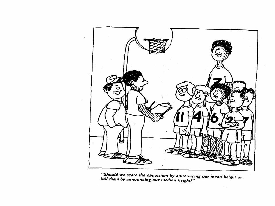
Mean or
Median?

Robust (Resistant) Statistic
Median is resistant to extreme values (outliers) in data set.
Mean is NOT robust against extreme values. Mean is pulled away from the center of the distribution toward the extreme value (“tails of graph”).
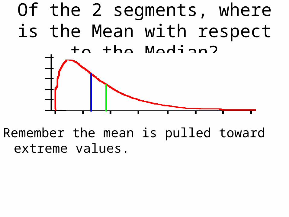
Of the 2 segments, where is the Mean with respect to the Median?
Remember the mean is pulled toward extreme values.

Where’s the Mean with respect to the Median?

Describing Spread: Standard DeviationRoughly speaking, standard deviation is the average distance values fall from the mean (center of graph).
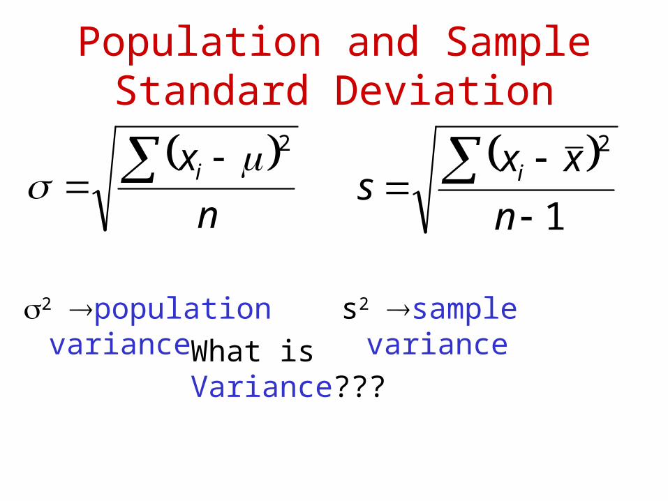
Population and SampleStandard Deviation
2 population variance s2 sample variance
n
xi
2
1
2
n
xxs i
What is Variance???

What is Variance?
Variance = (Standard deviation)2
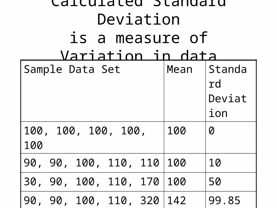
Calculated Standard Deviationis a measure of Variation in data
Sample Data Set Mean Standard Deviation
100, 100, 100, 100, 100 100 0
90, 90, 100, 110, 110 100 10
30, 90, 100, 110, 170 100 50
90, 90, 100, 110, 320 142 99.85

LET’S CUSS!

Center
Unusual Features
Spread
Shape
To describe a distribution:LET’S CUSS!

Center Mean, Median
Unusual Features Gaps, Outliers, Clusters
Spread Standard Deviation, Range, IQR
Shape Normal, Symmetric, Skewed Right (left)

CENTERMean(, ) —add up data values and divide by
number of data values
Median—list data values in order, locate middle data value
Data Set: 19, 20, 20, 21, 22
Mean is 04.205
2221202019
x
Median is 20 since it is the middle number of the ranked (ordered) data values.
x

Cluster---Gaps---Potential OutliersC
ou
nt
51015202530354045
Age_Husb_at_Marriage20 30 40 50 60
HusbandsAndWives Histogram
UNUSUAL FEATURES

SHAPE
Normal – bell-shaped Skewed Right
The shape can also be skewed left or symmetric or uniform.
“Tail” points to right

SPREAD
The spread can be described using: Standard Deviation (about 10) or
Range (80 – 150 or 70) orIQR (about 100 – 130)

Summary Features of Quantitative Variables
Center – Location
Unusual Features – Outliers, Gaps, Clusters
Spread – Variability
Shape – Distribution Pattern
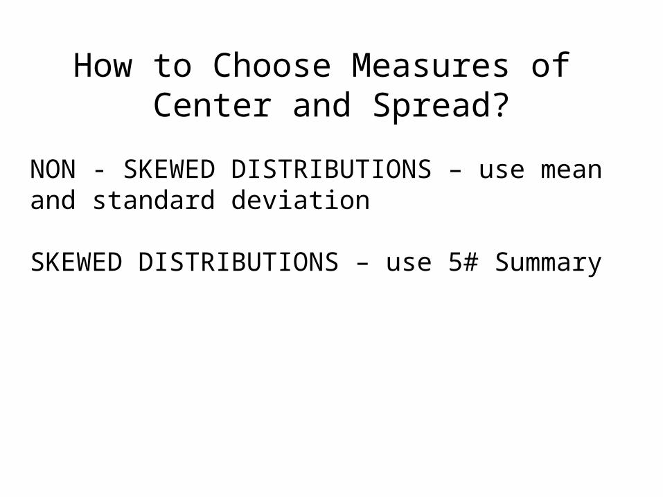
How to Choose Measures of Center and Spread?
NON - SKEWED DISTRIBUTIONS – use mean and standard deviation
SKEWED DISTRIBUTIONS – use 5# Summary

Comparing Distributions
• CUSS • COMPARE in CONTEXT• GENERAL CONCLUSION

Linear Transformationsusing the height of all LHS Seniors (in inches)
What happens to center and spread if everyone is put in 3 inch heels (add 3 inches)?
What happens to the center and spread if we change everyone height to feet (divide by 12)?

Summary of Linear Transformations
Multiplying each observation by a positive number b multiplies both measures of center (mean and median) and measures of spread (IQR and standard deviation) by b.
Adding the same number a (either positive, negative, or zero) to each observation adds a to measures of center and to quartiles but does not change measures of spread.
NOTE: The shape NEVER changes!