AP® Statistics 2009 Free-Response Questions - AP Central - The

AP® Statistics 2009 Free-Response Questions

The College Board

The College Board is a not-for-profit membership association whose mission is to connect students to college success and opportunity. Founded in 1900, the association is composed of more than 5,600 schools, colleges, universities and other educational organizations. Each year, the College Board serves seven million students and their parents, 23,000 high schools and 3,800 colleges through major programs and services in college readiness, college admissions, guidance, assessment, financial aid, enrollment, and teaching and learning. Among its best-known programs are the SAT®, the PSAT/NMSQT® and the Advanced Placement Program® (AP®). The College Board is committed to the principles of excellence and equity, and that commitment is embodied in all of its programs, services, activities and concerns.

© 2009 The College Board. All rights reserved. College Board, Advanced Placement Program, AP, AP Central, SAT, and the acorn logo are registered trademarks of the College Board. PSAT/NMSQT is a registered trademark of the College Board and National Merit Scholarship Corporation. Permission to use copyrighted College Board materials may be requested online at: www.collegeboard.com/inquiry/cbpermit.html. Visit the College Board on the Web: www.collegeboard.com. AP Central is the official online home for the AP Program: apcentral.collegeboard.com.

2009 AP® STATISTICS FREE-RESPONSE QUESTIONS

-2-

Formulas begin on page 3. Questions begin on page 6. Tables begin on page 11.


-3-

Formulas (I) Descriptive Statistics

xix

nÂ

=

( )211xs x xin

= -Â-

( ) ( )( ) ( )

2 21 21 2

1 2

1 1

1 1p

n s n ss

n n

- + -=

- + -

0 1y b b x= +

( )( )( )1 2

i i

i

x x y yb

x x

Â

Â

- -=

-

0 1b y b x= -

11

i i

x y

x x y yr

n s s

Ê ˆÊ ˆÂ Á ˜Á ˜Ë ¯ Ë ¯

- -= -

1y

x

sb r

s=

( )

( )

2

21

ˆ

2i i

b

i

y y

nsx x

Â

Â

--=-


-4-

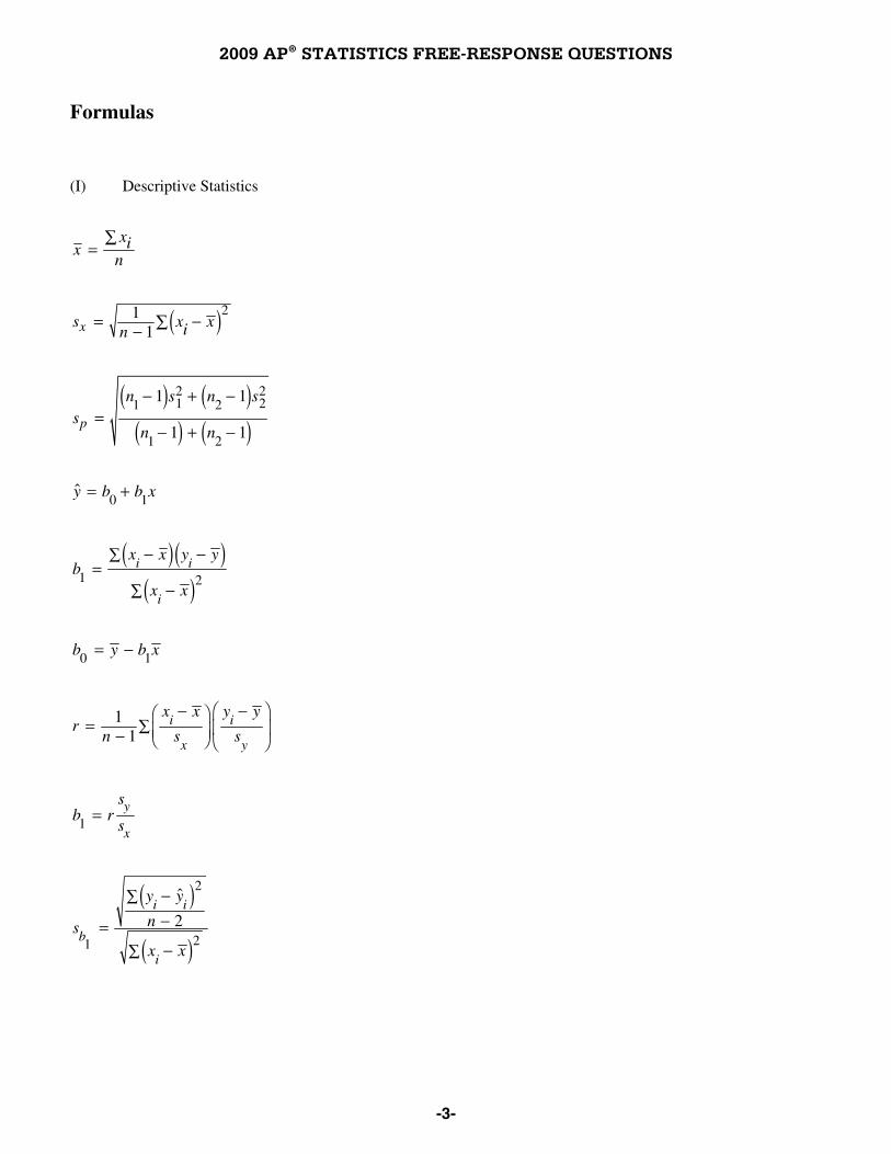
(II) Probability

( ) ( ) ( ) ( )P A B P A P B P A B» = + - «

( )

( )( )

P A BP A B

P B«=

( )E X x px i i= = Âμ

( )22Var( ) x i xX x pis= = -Â μ

If X has a binomial distribution with parameters n and p , then:

( ) (1 )n k n kP X k p pkÊ ˆÁ ˜Ë ¯

-= = -

npx =μ

(1 )np pxs = -

ˆ pp =μ

(1 )

ˆp p

p ns

-=

If x is the mean of a random sample of size n from an infinite population with mean μ and standard deviation ,s then:

x =μ μ

x ns

s =


-5-

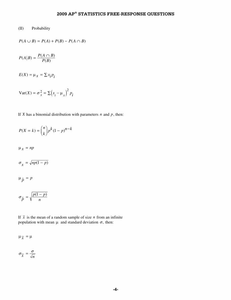
(III) Inferential Statistics

standard deviation of statisticstatistic parameter

Standardized test statistic:-

( ) ( )Confidence interval: statistic critical value standard deviation of statistic∑±

Single-Sample

Statistic Standard Deviation of Statistic

Sample Mean

ns

Sample Proportion

(1 )p pn-

Two-Sample

Statistic Standard Deviation of Statistic

Difference of sample means

2 21 2

1 2n ns s

+

Special case when 1 2s s=

1 2

1 1n n

s +

Difference of

sample proportions

1 1 2 2

1 2

(1 ) (1 )p p p pn n- -

+

Special case when 1 2p p=

( )1p p-1 2

1 1n n

+

( )2observed expectedChi-square test statistic

expected-

= Â


© 2009 The College Board. All rights reserved. Visit the College Board on the Web: www.collegeboard.com.

GO ON TO THE NEXT PAGE. -6-

STATISTICS SECTION II

Part A Questions 1-5

Spend about 65 minutes on this part of the exam. Percent of Section II score—75

Directions: Show all your work. Indicate clearly the methods you use, because you will be graded on the correctness of your methods as well as on the accuracy and completeness of your results and explanations. 1. A simple random sample of 100 high school seniors was selected from a large school district. The gender of each

student was recorded, and each student was asked the following questions.

1. Have you ever had a part-time job?

2. If you answered yes to the previous question, was your part-time job in the summer only?

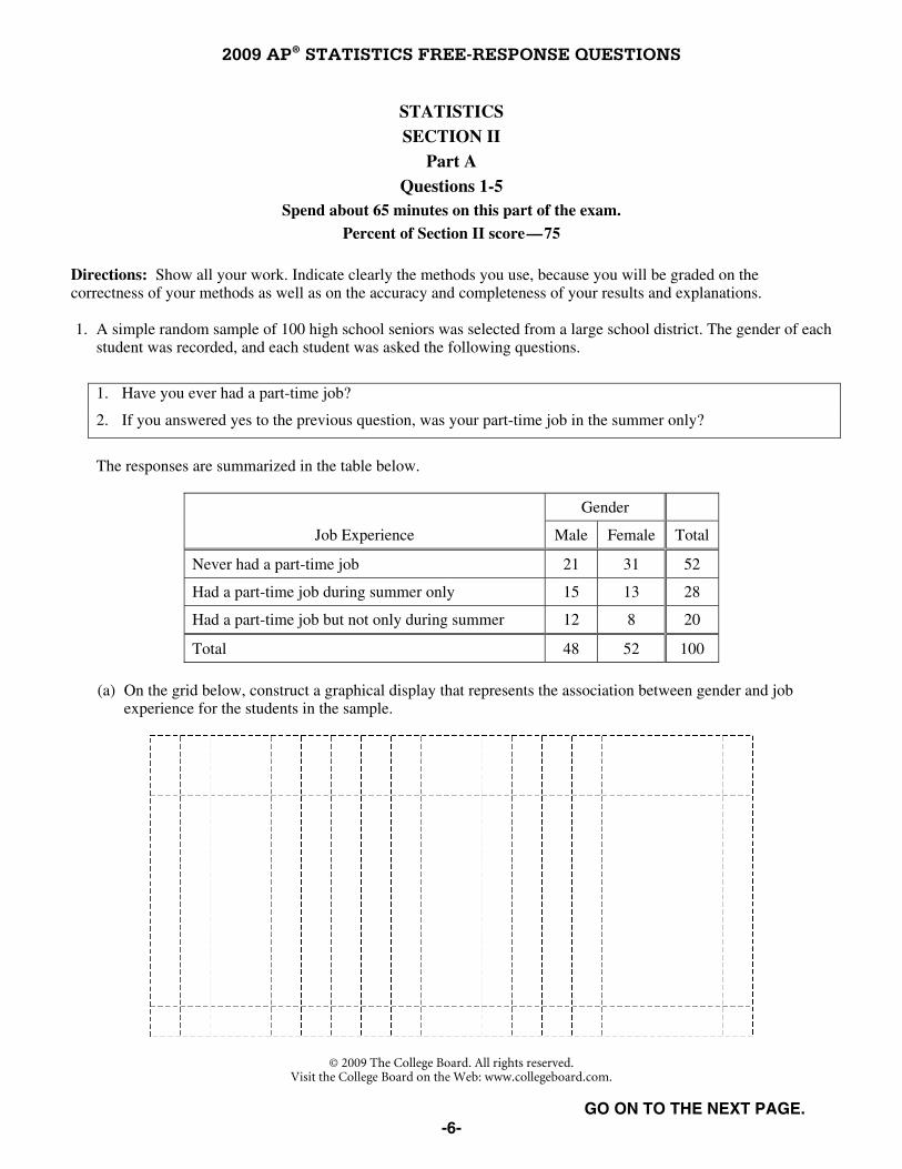
The responses are summarized in the table below.

Gender

Job Experience Male Female Total

Never had a part-time job 21 31 52

Had a part-time job during summer only 15 13 28

Had a part-time job but not only during summer 12 8 20

Total 48 52 100

(a) On the grid below, construct a graphical display that represents the association between gender and job

experience for the students in the sample.




(b) Write a few sentences summarizing what the display in part (a) reveals about the association between gender and job experience for the students in the sample.

(c) Which test of significance should be used to test if there is an association between gender and job experience for the population of high school seniors in the district?

State the null and alternative hypotheses for the test, but do not perform the test.

2. A tire manufacturer designed a new tread pattern for its all-weather tires. Repeated tests were conducted on cars

of approximately the same weight traveling at 60 miles per hour. The tests showed that the new tread pattern enables the cars to stop completely in an average distance of 125 feet with a standard deviation of 6.5 feet and that the stopping distances are approximately normally distributed.

(a) What is the 70th percentile of the distribution of stopping distances?

(b) What is the probability that at least 2 cars out of 5 randomly selected cars in the study will stop in a distance that is greater than the distance calculated in part (a) ?

(c) What is the probability that a randomly selected sample of 5 cars in the study will have a mean stopping distance of at least 130 feet?

3. Before beginning a unit on frog anatomy, a seventh-grade biology teacher gives each of the 24 students in the

class a pretest to assess their knowledge of frog anatomy. The teacher wants to compare the effectiveness of an instructional program in which students physically dissect frogs with the effectiveness of a different program in which students use computer software that only simulates the dissection of a frog. After completing one of the two programs, students will be given a posttest to assess their knowledge of frog anatomy. The teacher will then analyze the changes in the test scores (score on posttest minus score on pretest).

(a) Describe a method for assigning the 24 students to two groups of equal size that allows for a statistically

valid comparison of the two instructional programs.

(b) Suppose the teacher decided to allow the students in the class to select which instructional program on frog anatomy (physical dissection or computer simulation) they prefer to take, and 11 students choose actual dissection and 13 students choose computer simulation. How might that self-selection process jeopardize a statistically valid comparison of the changes in the test scores (score on posttest minus score on pretest) for the two instructional programs? Provide a specific example to support your answer.




4. One of the two fire stations in a certain town responds to calls in the northern half of the town, and the other fire station responds to calls in the southern half of the town. One of the town council members believes that the two fire stations have different mean response times. Response time is measured by the difference between the time an emergency call comes into the fire station and the time the first fire truck arrives at the scene of the fire.

Data were collected to investigate whether the council member’s belief is correct. A random sample of 50 calls selected from the northern fire station had a mean response time of 4.3 minutes with a standard deviation of 3.7 minutes. A random sample of 50 calls selected from the southern fire station had a mean response time of 5.3 minutes with a standard deviation of 3.2 minutes.

(a) Construct and interpret a 95 percent confidence interval for the difference in mean response times between

the two fire stations.

(b) Does the confidence interval in part (a) support the council member’s belief that the two fire stations have different mean response times? Explain.

5. For many years, the medically accepted practice of giving aid to a person experiencing a heart attack was to have

the person who placed the emergency call administer chest compression (CC) plus standard mouth-to-mouth resuscitation (MMR) to the heart attack patient until the emergency response team arrived. However, some researchers believed that CC alone would be a more effective approach.

In the 1990s a study was conducted in Seattle in which 518 cases were randomly assigned to treatments: 278 to CC plus standard MMR and 240 to CC alone. A total of 64 patients survived the heart attack: 29 in the group receiving CC plus standard MMR, and 35 in the group receiving CC alone. A test of significance was conducted on the following hypotheses.

0H : The survival rates for the two treatments are equal.

H :a The treatment that uses CC alone produces a higher survival rate.

This test resulted in a p-value of 0.0761.

(a) Interpret what this p-value measures in the context of this study.

(b) Based on this p-value and study design, what conclusion should be drawn in the context of this study? Use a significance level of α = 0.05.

(c) Based on your conclusion in part (b), which type of error, Type I or Type II, could have been made? What is one potential consequence of this error?




STATISTICS SECTION II

Part B Question 6

Spend about 25 minutes on this part of the exam. Percent of Section II score—25

Directions: Show all your work. Indicate clearly the methods you use, because you will be graded on the correctness of your methods as well as on the accuracy and completeness of your results and explanations. 6. A consumer organization was concerned that an automobile manufacturer was misleading customers by

overstating the average fuel efficiency (measured in miles per gallon, or mpg) of a particular car model. The model was advertised to get 27 mpg. To investigate, researchers selected a random sample of 10 cars of that model. Each car was then randomly assigned a different driver. Each car was driven for 5,000 miles, and the total fuel consumption was used to compute mpg for that car.

(a) Define the parameter of interest and state the null and alternative hypotheses the consumer organization is

interested in testing.

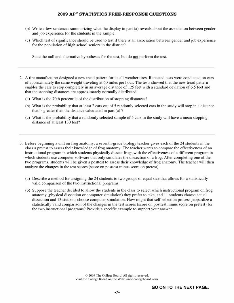
One condition for conducting a one-sample t-test in this situation is that the mpg measurements for the population of cars of this model should be normally distributed. However, the boxplot and histogram shown below indicate that the distribution of the 10 sample values is skewed to the right.

(b) One possible statistic that measures skewness is the ratio sample mean

sample median. What values of that statistic

(small, large, close to one) might indicate that the population distribution of mpg values is skewed to the right? Explain.



-10-

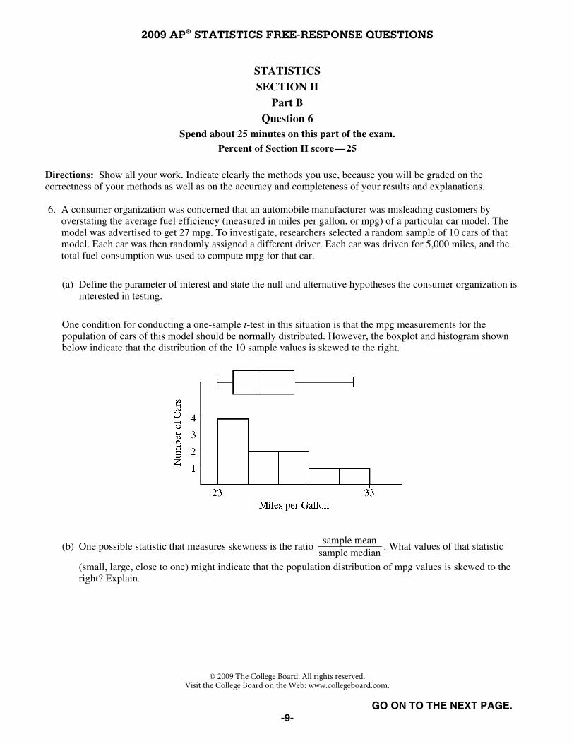
(c) Even though the mpg values in the sample were skewed to the right, it is still possible that the population distribution of mpg values is normally distributed and that the skewness was due to sampling variability. To investigate, 100 samples, each of size 10, were taken from a normal distribution with the same mean and

standard deviation as the original sample. For each of those 100 samples, the statistic sample mean

sample median was

calculated. A dotplot of the 100 simulated statistics is shown below.

In the original sample, the value of the statistic sample mean

sample median was 1.03. Based on the value of 1.03 and

the dotplot above, is it plausible that the original sample of 10 cars came from a normal population, or do the simulated results suggest the original population is really skewed to the right? Explain.

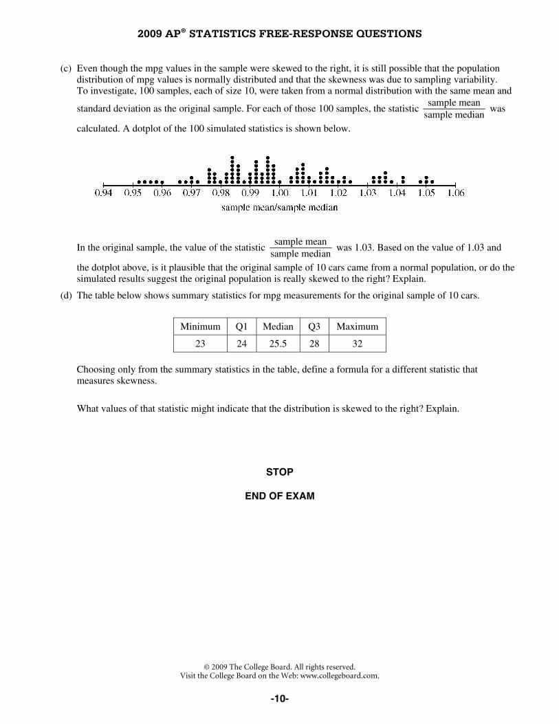
(d) The table below shows summary statistics for mpg measurements for the original sample of 10 cars.

Minimum Q1 Median Q3 Maximum

23 24 25.5 28 32

Choosing only from the summary statistics in the table, define a formula for a different statistic that

measures skewness.

What values of that statistic might indicate that the distribution is skewed to the right? Explain.

STOP

END OF EXAM


-11-

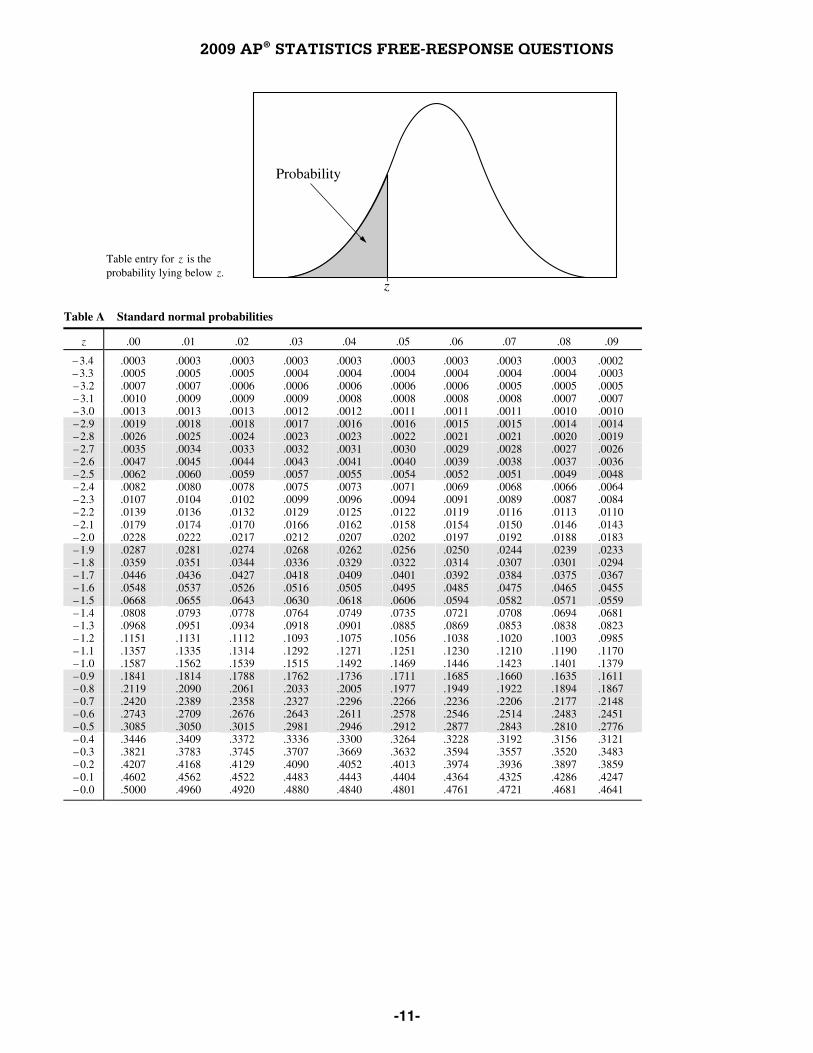
Probability

z

Table A Standard normal probabilities

z .00 .01 .02 .03 .04 .05 .06 .07 .08 .09 –3.4 .0003 .0003 .0003 .0003 .0003 .0003 .0003 .0003 .0003 .0002 –3.3 .0005 .0005 .0005 .0004 .0004 .0004 .0004 .0004 .0004 .0003 –3.2 .0007 .0007 .0006 .0006 .0006 .0006 .0006 .0005 .0005 .0005 –3.1 .0010 .0009 .0009 .0009 .0008 .0008 .0008 .0008 .0007 .0007 –3.0 .0013 .0013 .0013 .0012 .0012 .0011 .0011 .0011 .0010 .0010 –2.9 .0019 .0018 .0018 .0017 .0016 .0016 .0015 .0015 .0014 .0014 –2.8 .0026 .0025 .0024 .0023 .0023 .0022 .0021 .0021 .0020 .0019 –2.7 .0035 .0034 .0033 .0032 .0031 .0030 .0029 .0028 .0027 .0026 –2.6 .0047 .0045 .0044 .0043 .0041 .0040 .0039 .0038 .0037 .0036 –2.5 .0062 .0060 .0059 .0057 .0055 .0054 .0052 .0051 .0049 .0048 –2.4 .0082 .0080 .0078 .0075 .0073 .0071 .0069 .0068 .0066 .0064 –2.3 .0107 .0104 .0102 .0099 .0096 .0094 .0091 .0089 .0087 .0084 –2.2 .0139 .0136 .0132 .0129 .0125 .0122 .0119 .0116 .0113 .0110 –2.1 .0179 .0174 .0170 .0166 .0162 .0158 .0154 .0150 .0146 .0143 –2.0 .0228 .0222 .0217 .0212 .0207 .0202 .0197 .0192 .0188 .0183 –1.9 .0287 .0281 .0274 .0268 .0262 .0256 .0250 .0244 .0239 .0233 –1.8 .0359 .0351 .0344 .0336 .0329 .0322 .0314 .0307 .0301 .0294 –1.7 .0446 .0436 .0427 .0418 .0409 .0401 .0392 .0384 .0375 .0367 –1.6 .0548 .0537 .0526 .0516 .0505 .0495 .0485 .0475 .0465 .0455 –1.5 .0668 .0655 .0643 .0630 .0618 .0606 .0594 .0582 .0571 .0559 –1.4 .0808 .0793 .0778 .0764 .0749 .0735 .0721 .0708 .0694 .0681 –1.3 .0968 .0951 .0934 .0918 .0901 .0885 .0869 .0853 .0838 .0823 –1.2 .1151 .1131 .1112 .1093 .1075 .1056 .1038 .1020 .1003 .0985 –1.1 .1357 .1335 .1314 .1292 .1271 .1251 .1230 .1210 .1190 .1170 –1.0 .1587 .1562 .1539 .1515 .1492 .1469 .1446 .1423 .1401 .1379 –0.9 .1841 .1814 .1788 .1762 .1736 .1711 .1685 .1660 .1635 .1611 –0.8 .2119 .2090 .2061 .2033 .2005 .1977 .1949 .1922 .1894 .1867 –0.7 .2420 .2389 .2358 .2327 .2296 .2266 .2236 .2206 .2177 .2148 –0.6 .2743 .2709 .2676 .2643 .2611 .2578 .2546 .2514 .2483 .2451 –0.5 .3085 .3050 .3015 .2981 .2946 .2912 .2877 .2843 .2810 .2776 –0.4 .3446 .3409 .3372 .3336 .3300 .3264 .3228 .3192 .3156 .3121 –0.3 .3821 .3783 .3745 .3707 .3669 .3632 .3594 .3557 .3520 .3483 –0.2 .4207 .4168 .4129 .4090 .4052 .4013 .3974 .3936 .3897 .3859 –0.1 .4602 .4562 .4522 .4483 .4443 .4404 .4364 .4325 .4286 .4247 –0.0 .5000 .4960 .4920 .4880 .4840 .4801 .4761 .4721 .4681 .4641

Table entry for z is the probability lying below z.


-12-

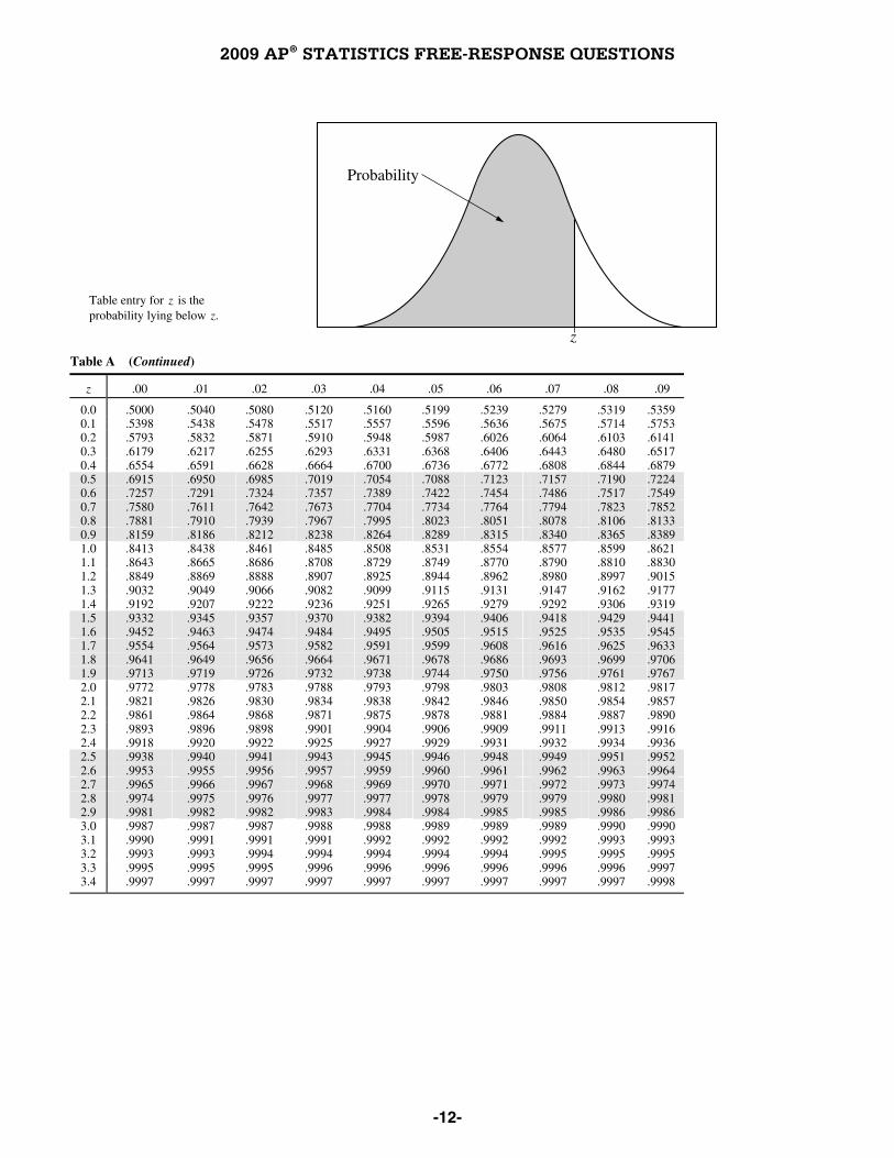
Probability

z

Table A (Continued)

z .00 .01 .02 .03 .04 .05 .06 .07 .08 .09 0.0 .5000 .5040 .5080 .5120 .5160 .5199 .5239 .5279 .5319 .5359 0.1 .5398 .5438 .5478 .5517 .5557 .5596 .5636 .5675 .5714 .5753 0.2 .5793 .5832 .5871 .5910 .5948 .5987 .6026 .6064 .6103 .6141 0.3 .6179 .6217 .6255 .6293 .6331 .6368 .6406 .6443 .6480 .6517 0.4 .6554 .6591 .6628 .6664 .6700 .6736 .6772 .6808 .6844 .6879 0.5 .6915 .6950 .6985 .7019 .7054 .7088 .7123 .7157 .7190 .7224 0.6 .7257 .7291 .7324 .7357 .7389 .7422 .7454 .7486 .7517 .7549 0.7 .7580 .7611 .7642 .7673 .7704 .7734 .7764 .7794 .7823 .7852 0.8 .7881 .7910 .7939 .7967 .7995 .8023 .8051 .8078 .8106 .8133 0.9 .8159 .8186 .8212 .8238 .8264 .8289 .8315 .8340 .8365 .8389 1.0 .8413 .8438 .8461 .8485 .8508 .8531 .8554 .8577 .8599 .8621 1.1 .8643 .8665 .8686 .8708 .8729 .8749 .8770 .8790 .8810 .8830 1.2 .8849 .8869 .8888 .8907 .8925 .8944 .8962 .8980 .8997 .9015 1.3 .9032 .9049 .9066 .9082 .9099 .9115 .9131 .9147 .9162 .9177 1.4 .9192 .9207 .9222 .9236 .9251 .9265 .9279 .9292 .9306 .9319 1.5 .9332 .9345 .9357 .9370 .9382 .9394 .9406 .9418 .9429 .9441 1.6 .9452 .9463 .9474 .9484 .9495 .9505 .9515 .9525 .9535 .9545 1.7 .9554 .9564 .9573 .9582 .9591 .9599 .9608 .9616 .9625 .9633 1.8 .9641 .9649 .9656 .9664 .9671 .9678 .9686 .9693 .9699 .9706 1.9 .9713 .9719 .9726 .9732 .9738 .9744 .9750 .9756 .9761 .9767 2.0 .9772 .9778 .9783 .9788 .9793 .9798 .9803 .9808 .9812 .9817 2.1 .9821 .9826 .9830 .9834 .9838 .9842 .9846 .9850 .9854 .9857 2.2 .9861 .9864 .9868 .9871 .9875 .9878 .9881 .9884 .9887 .9890 2.3 .9893 .9896 .9898 .9901 .9904 .9906 .9909 .9911 .9913 .9916 2.4 .9918 .9920 .9922 .9925 .9927 .9929 .9931 .9932 .9934 .9936 2.5 .9938 .9940 .9941 .9943 .9945 .9946 .9948 .9949 .9951 .9952 2.6 .9953 .9955 .9956 .9957 .9959 .9960 .9961 .9962 .9963 .9964 2.7 .9965 .9966 .9967 .9968 .9969 .9970 .9971 .9972 .9973 .9974 2.8 .9974 .9975 .9976 .9977 .9977 .9978 .9979 .9979 .9980 .9981 2.9 .9981 .9982 .9982 .9983 .9984 .9984 .9985 .9985 .9986 .9986 3.0 .9987 .9987 .9987 .9988 .9988 .9989 .9989 .9989 .9990 .9990 3.1 .9990 .9991 .9991 .9991 .9992 .9992 .9992 .9992 .9993 .9993 3.2 .9993 .9993 .9994 .9994 .9994 .9994 .9994 .9995 .9995 .9995 3.3 .9995 .9995 .9995 .9996 .9996 .9996 .9996 .9996 .9996 .9997 3.4 .9997 .9997 .9997 .9997 .9997 .9997 .9997 .9997 .9997 .9998

Table entry for z is the probability lying below z.


-13-

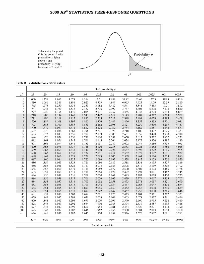
Probability p

t*

Table B t distribution critical values

Tail probability p

df .25 .20 .15 .10 .05 .025 .02 .01 .005 .0025 .001 .0005

1 1.000 1.376 1.963 3.078 6.314 12.71 15.89 31.82 63.66 127.3 318.3 636.6 2 .816 1.061 1.386 1.886 2.920 4.303 4.849 6.965 9.925 14.09 22.33 31.60 3 .765 .978 1.250 1.638 2.353 3.182 3.482 4.541 5.841 7.453 10.21 12.92 4 .741 .941 1.190 1.533 2.132 2.776 2.999 3.747 4.604 5.598 7.173 8.610 5 .727 .920 1.156 1.476 2.015 2.571 2.757 3.365 4.032 4.773 5.893 6.869 6 .718 .906 1.134 1.440 1.943 2.447 2.612 3.143 3.707 4.317 5.208 5.959 7 .711 .896 1.119 1.415 1.895 2.365 2.517 2.998 3.499 4.029 4.785 5.408 8 .706 .889 1.108 1.397 1.860 2.306 2.449 2.896 3.355 3.833 4.501 5.041 9 .703 .883 1.100 1.383 1.833 2.262 2.398 2.821 3.250 3.690 4.297 4.781

10 .700 .879 1.093 1.372 1.812 2.228 2.359 2.764 3.169 3.581 4.144 4.587 11 .697 .876 1.088 1.363 1.796 2.201 2.328 2.718 3.106 3.497 4.025 4.437 12 .695 .873 1.083 1.356 1.782 2.179 2.303 2.681 3.055 3.428 3.930 4.318 13 .694 .870 1.079 1.350 1.771 2.160 2.282 2.650 3.012 3.372 3.852 4.221 14 .692 .868 1.076 1.345 1.761 2.145 2.264 2.624 2.977 3.326 3.787 4.140 15 .691 .866 1.074 1.341 1.753 2.131 2.249 2.602 2.947 3.286 3.733 4.073 16 .690 .865 1.071 1.337 1.746 2.120 2.235 2.583 2.921 3.252 3.686 4.015 17 .689 .863 1.069 1.333 1.740 2.110 2.224 2.567 2.898 3.222 3.646 3.965 18 .688 .862 1.067 1.330 1.734 2.101 2.214 2.552 2.878 3.197 3.611 3.922 19 .688 .861 1.066 1.328 1.729 2.093 2.205 2.539 2.861 3.174 3.579 3.883 20 .687 .860 1.064 1.325 1.725 2.086 2.197 2.528 2.845 3.153 3.552 3.850 21 .686 .859 1.063 1.323 1.721 2.080 2.189 2.518 2.831 3.135 3.527 3.819 22 .686 .858 1.061 1.321 1.717 2.074 2.183 2.508 2.819 3.119 3.505 3.792 23 .685 .858 1.060 1.319 1.714 2.069 2.177 2.500 2.807 3.104 3.485 3.768 24 .685 .857 1.059 1.318 1.711 2.064 2.172 2.492 2.797 3.091 3.467 3.745 25 .684 .856 1.058 1.316 1.708 2.060 2.167 2.485 2.787 3.078 3.450 3.725 26 .684 .856 1.058 1.315 1.706 2.056 2.162 2.479 2.779 3.067 3.435 3.707 27 .684 .855 1.057 1.314 1.703 2.052 2.158 2.473 2.771 3.057 3.421 3.690 28 .683 .855 1.056 1.313 1.701 2.048 2.154 2.467 2.763 3.047 3.408 3.674 29 .683 .854 1.055 1.311 1.699 2.045 2.150 2.462 2.756 3.038 3.396 3.659 30 .683 .854 1.055 1.310 1.697 2.042 2.147 2.457 2.750 3.030 3.385 3.646 40 .681 .851 1.050 1.303 1.684 2.021 2.123 2.423 2.704 2.971 3.307 3.551 50 .679 .849 1.047 1.299 1.676 2.009 2.109 2.403 2.678 2.937 3.261 3.496 60 .679 .848 1.045 1.296 1.671 2.000 2.099 2.390 2.660 2.915 3.232 3.460 80 .678 .846 1.043 1.292 1.664 1.990 2.088 2.374 2.639 2.887 3.195 3.416

100 .677 .845 1.042 1.290 1.660 1.984 2.081 2.364 2.626 2.871 3.174 3.390 1000 .675 .842 1.037 1.282 1.646 1.962 2.056 2.330 2.581 2.813 3.098 3.300

� .674 .841 1.036 1.282 1.645 1.960 2.054 2.326 2.576 2.807 3.091 3.291

50% 60% 70% 80% 90% 95% 96% 98% 99% 99.5% 99.8% 99.9%

Confidence level C

Table entry for p and C is the point t* with probability p lying above it and probability C lying between −t * and t*.


-14-

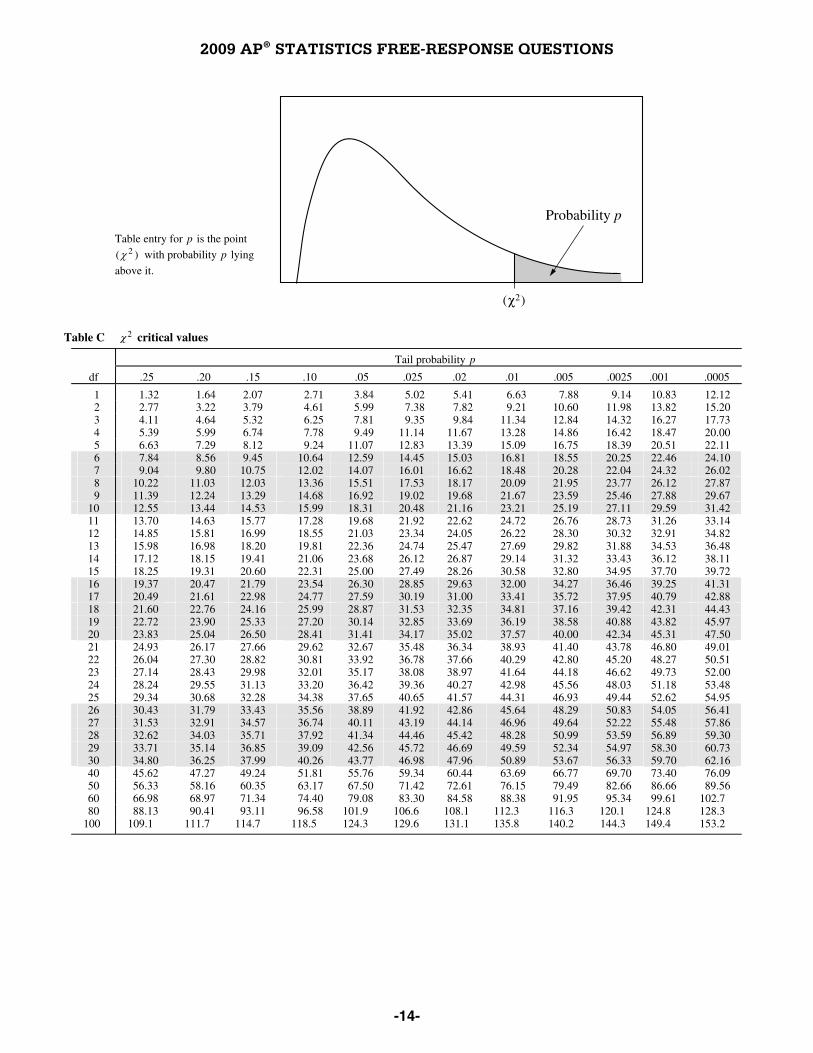
Probability p

(χ2)

Table C 2c critical values Tail probability p

df .25 .20 .15 .10 .05 .025 .02 .01 .005 .0025 .001 .0005

1 1.32 1.64 2.07 2.71 3.84 5.02 5.41 6.63 7.88 9.14 10.83 12.12 2 2.77 3.22 3.79 4.61 5.99 7.38 7.82 9.21 10.60 11.98 13.82 15.20 3 4.11 4.64 5.32 6.25 7.81 9.35 9.84 11.34 12.84 14.32 16.27 17.73 4 5.39 5.99 6.74 7.78 9.49 11.14 11.67 13.28 14.86 16.42 18.47 20.00 5 6.63 7.29 8.12 9.24 11.07 12.83 13.39 15.09 16.75 18.39 20.51 22.11 6 7.84 8.56 9.45 10.64 12.59 14.45 15.03 16.81 18.55 20.25 22.46 24.10 7 9.04 9.80 10.75 12.02 14.07 16.01 16.62 18.48 20.28 22.04 24.32 26.02 8 10.22 11.03 12.03 13.36 15.51 17.53 18.17 20.09 21.95 23.77 26.12 27.87 9 11.39 12.24 13.29 14.68 16.92 19.02 19.68 21.67 23.59 25.46 27.88 29.67

10 12.55 13.44 14.53 15.99 18.31 20.48 21.16 23.21 25.19 27.11 29.59 31.42 11 13.70 14.63 15.77 17.28 19.68 21.92 22.62 24.72 26.76 28.73 31.26 33.14 12 14.85 15.81 16.99 18.55 21.03 23.34 24.05 26.22 28.30 30.32 32.91 34.82 13 15.98 16.98 18.20 19.81 22.36 24.74 25.47 27.69 29.82 31.88 34.53 36.48 14 17.12 18.15 19.41 21.06 23.68 26.12 26.87 29.14 31.32 33.43 36.12 38.11 15 18.25 19.31 20.60 22.31 25.00 27.49 28.26 30.58 32.80 34.95 37.70 39.72 16 19.37 20.47 21.79 23.54 26.30 28.85 29.63 32.00 34.27 36.46 39.25 41.31 17 20.49 21.61 22.98 24.77 27.59 30.19 31.00 33.41 35.72 37.95 40.79 42.88 18 21.60 22.76 24.16 25.99 28.87 31.53 32.35 34.81 37.16 39.42 42.31 44.43 19 22.72 23.90 25.33 27.20 30.14 32.85 33.69 36.19 38.58 40.88 43.82 45.97 20 23.83 25.04 26.50 28.41 31.41 34.17 35.02 37.57 40.00 42.34 45.31 47.50 21 24.93 26.17 27.66 29.62 32.67 35.48 36.34 38.93 41.40 43.78 46.80 49.01 22 26.04 27.30 28.82 30.81 33.92 36.78 37.66 40.29 42.80 45.20 48.27 50.51 23 27.14 28.43 29.98 32.01 35.17 38.08 38.97 41.64 44.18 46.62 49.73 52.00 24 28.24 29.55 31.13 33.20 36.42 39.36 40.27 42.98 45.56 48.03 51.18 53.48 25 29.34 30.68 32.28 34.38 37.65 40.65 41.57 44.31 46.93 49.44 52.62 54.95 26 30.43 31.79 33.43 35.56 38.89 41.92 42.86 45.64 48.29 50.83 54.05 56.41 27 31.53 32.91 34.57 36.74 40.11 43.19 44.14 46.96 49.64 52.22 55.48 57.86 28 32.62 34.03 35.71 37.92 41.34 44.46 45.42 48.28 50.99 53.59 56.89 59.30 29 33.71 35.14 36.85 39.09 42.56 45.72 46.69 49.59 52.34 54.97 58.30 60.73 30 34.80 36.25 37.99 40.26 43.77 46.98 47.96 50.89 53.67 56.33 59.70 62.16 40 45.62 47.27 49.24 51.81 55.76 59.34 60.44 63.69 66.77 69.70 73.40 76.09 50 56.33 58.16 60.35 63.17 67.50 71.42 72.61 76.15 79.49 82.66 86.66 89.56 60 66.98 68.97 71.34 74.40 79.08 83.30 84.58 88.38 91.95 95.34 99.61 102.7 80 88.13 90.41 93.11 96.58 101.9 106.6 108.1 112.3 116.3 120.1 124.8 128.3

100 109.1 111.7 114.7 118.5 124.3 129.6 131.1 135.8 140.2 144.3 149.4 153.2

Table entry for p is the point

( )χ 2 with probability p lying

above it.

Documents

AP® Statistics 2009 Free-Response Questions - AP Central - The