Embed Size (px)
Citation preview

Course Planning and Pacing Guide
AP® Calculus BC
Mark HowellGonzaga College High School ▶ Washington, DC
© 2015 The College Board. College Board, Advanced Placement Program, AP, AP Central, SAT and the acorn logo are registered trademarks of the College Board. All other products and services may be trademarks of their respective owners. Visit the College Board on the Web: www.collegeboard.org.

AP Calculus BC ■ Course Planning and Pacing Guide ■ Mark Howell © 2015 The College Board. i
About the College BoardThe College Board is a mission-driven not-for-profit organization that connects students to college success and opportunity. Founded in 1900, the College Board was created to expand access to higher education. Today, the membership association is made up of over 6,000 of the world’s leading educational institutions and is dedicated to promoting excellence and equity in education. Each year, the College Board helps more than seven million students prepare for a successful transition to college through programs and services in college readiness and college success — including the SAT® and the Advanced Placement Program®. The organization also serves the education community through research and advocacy on behalf of students, educators, and schools. For further information, visit www.collegeboard.org.
AP® Equity and Access PolicyThe College Board strongly encourages educators to make equitable access a guiding principle for their AP® programs by giving all willing and academically prepared students the opportunity to participate in AP. We encourage the elimination of barriers that restrict access to AP for students from ethnic, racial, and socioeconomic groups that have been traditionally underrepresented. Schools should make every effort to ensure their AP classes reflect the diversity of their student population. The College Board also believes that all students should have access to academically challenging course work before they enroll in AP classes, which can prepare them for AP success. It is only through a commitment to equitable preparation and access that true equity and excellence can be achieved.
Welcome to the AP Calculus BC Course Planning and Pacing GuidesThis guide is one of several course planning and pacing guides designed for AP Calculus BC teachers. Each provides an example of how to design instruction for the AP course based on the author’s teaching context (e.g., demographics, schedule, school type, setting). These course planning and pacing guides highlight how the components of the AP Calculus AB and BC Curriculum Framework, which uses an Understanding by Design approach, are addressed in the course. Each guide also provides valuable suggestions for teaching the course, including the selection of resources, instructional activities, and assessments. The authors have offered insight into the why and how behind their instructional choices — displayed along the right side of the individual unit plans — to aid in course planning for AP Calculus teachers.
The primary purpose of these comprehensive guides is to model approaches for planning and pacing curriculum throughout the school year. However, they can also help with syllabus development when used in conjunction with the resources created to support the AP Course Audit: the Syllabus Development Guide and the four Annotated Sample Syllabi. These resources include samples of evidence and illustrate a variety of strategies for meeting curricular requirements.

AP Calculus BC ■ Course Planning and Pacing Guide ■ Mark Howell © 2015 The College Board. ii
1 Instructional Setting
3 Overview of the Course
4 Mathematical Thinking Practices for AP Calculus (MPACs)
6 Pacing Overview
Course Planning and Pacing by Unit
8 Unit 1: Limits and Continuity
14 Unit 2: Defining and Calculating Derivatives
19 Unit 3: Applications of the Derivative
25 Unit 4: The Integral and the Fundamental Theorem of Calculus
30 Unit 5: Differential Equations
36 Unit 6: Applications of the Definite Integral
40 Unit 7: Sequences, L’Hospital’s Rule, and Improper Integrals
44 Unit 8: Series
52 Unit 9: Parametric and Polar Functions
56 Resources
Contents
AP Calculus BC ■ Course Planning and Pacing Guide ■ Mark Howell © 2015 The College Board. 1
Gonzaga College High School ▶ Washington, DC
School Gonzaga College High School is a Jesuit private high school for boys located in Washington, D.C.
Student population
Gonzaga is a selective school with a highly motivated student population of about 950 boys. Nearly all of our students go on to attend a four-year college. Approximately 23 percent of the population are minorities and about 33 percent receive some form of financial aid.
Instructional time
School starts around August 20. However, our AP Calculus BC course extends over three semesters. There are approximately 215 class days, spanning two academic years, prior to the AP Calculus Exam. The pacing guide presented here has been adjusted to accommodate a two-semester timeline, consisting of 142 days. Regular class periods are 40 minutes. About once every 10 days, each class meets for 70 minutes, which allows for regular extended lab activities.
Student preparation
Most students in AP Calculus BC have followed a three-semester sequence beginning with one semester of Advanced Geometry, followed by two semesters of Advanced Precalculus. These students skip Algebra II; the content usually covered in that class is covered in Precalculus. Some students begin the sequence in grade 9, some in grade 10, and others join the Calculus BC course after completing AP Calculus AB in grade 11.
Instructional Setting

AP Calculus BC ■ Course Planning and Pacing Guide ■ Mark Howell © 2015 The College Board. 2
Primary planning resources
Finney, Ross L., Franklin D. Demana, Bert K. Waits, and Daniel Kennedy. Calculus: Graphical, Numerical, Algebraic AP Edition. 4th ed. Boston, MA: Pearson, 2012.
Primary textbook.
Hughes-Hallett, Deborah, et al. Calculus: Single Variable. 6th ed. Hoboken, NJ: Wiley, 2013.
Used as a resource for conceptual problems that serve as prompts for journal questions (Strengthen Your Understanding questions in the textbook), as well as problems involving interpretations of the derivative and the integral.
Hughes-Hallett, Deborah, Guadalupe I. Lonzano, Andrew M. Gleason, et al. AP Guide for Calculus: Single Variable. Hoboken, NJ: Wiley, 2010.
This guide serves as a resource for several calculator activities, including those on tangent line errors and Taylor polynomial errors. It is also a resource for AP-style review questions. Available online at http://bcs.wiley.com/he-bcs/Books?action=resource&bcsId=7694&itemId=047088861X&resourceId=29852.
Antinone, Linda, Thomas Dick, Kevin Fitzpatrick, Michael Grasse, and Mark Howell. Calculus Activities: TI-83 Plus/TI-84 Plus Explorations. Texas Instruments, 2004. Available online at http://education.ti.com/en/us/activities/explorations-series-books/activitybook_calculus_activities.
This is used as a resource for lab activities throughout the course.
Howell, Mark, and Martha Montgomery. Be Prepared for the AP Calculus Exam. 2nd ed. Andover, MA: Skylight, 2011.
I use this AP Exam preparation book both during the review leading up to the exam and for review of individual instructional units.
“Free-Response Questions.” The College Board AP Central, AP Calculus BC. Accessed April 20, 2015. http://apcentral.collegeboard.com/apc/members/exam/exam_information/8031.html.
Instructional Setting (continued)

AP Calculus BC ■ Course Planning and Pacing Guide ■ Mark Howell © 2015 The College Board. 3
Students learn best by doing. Formation of knowledge about mathematics requires engagement with mathematics itself as a live, ongoing human endeavor. In teaching AP Calculus, I am guided by the idea that students need to form their own knowledge through activities where they get their hands dirty, where they scrape up against or run headlong into the deep and difficult ideas in calculus. In each major content area, I use activities as guided inquiries into the concepts at the core of calculus: the idea of limits, the notion of instantaneous rate of change (the derivative), and the idea of accumulation of a rate of change (the integral). Other activities offer real-world settings where calculus ideas are interpreted, or provide a setting for discovery of some deep connections among various ideas in calculus. In particular, the discovery activity of the fundamental theorem is a central conceptual component of the course. Two activities, one that explores the accuracy of tangent line approximations early in the course, and a similar one that explores the accuracy of polynomial approximations when we get to Taylor polynomials, serve as conceptual bookends for the course. Both of these help students understand one of the toughest results in AP Calculus, Taylor’s theorem.
Throughout the course, several concepts serve as unifying touchstones. The idea of limits recurs throughout the course in the definitions of asymptotes, continuity, the derivative, the integral, and convergence of infinite series. Local linearity comes up throughout the course as well. Differentiable functions have graphs that resemble straight lines when you look at them close up. In many important ways, they behave like straight lines. Tangent line approximations, midpoint Riemann sums, slope fields, Euler’s method, and even Taylor series all leverage the idea of local linearity.
There are four ways to represent functions: graphically, numerically, symbolically, and verbally. I make a deliberate effort to use all four regularly throughout the course, during in-class activities, assignments, tests, and quizzes. For example, when we begin studying the derivative, we zoom into the graph of a function while calculating the average rate of change of the function over ever-narrowing intervals. Students see and connect two facets of the same idea: the graph straightening out and the difference quotients that represent the average rate of change converging to a limiting value. Later, we tie the symbolic definition of the derivative at a point to this activity.
Finally, in response to a journal question, students write about these connections. In class, we make the conceptual connection among the three representations explicit by verbalizing how zooming into the graph results in an appearance of linearity, which is connected to slopes converging to a constant. And the idea of zooming in is tied to the Dx (or h) approaching 0 in the definition of derivative (see the instructional activity “Zooming In to Reveal Local Linearity” in Unit 2 for details).
Students keep a calculus journal in which they write about their understanding of concepts, and respond to my prompts. The question described above is one example. This sort of activity serves as a formative assessment. Depending on how well students grasp fundamental concepts I craft additional questions and activities to address deficiencies. I collect and grade the journals twice each semester. Journal grades are based more on the quality and frequency of the students’ writing than on mathematical correctness.
Several of the activities I use have sections for further exploration to accommodate interested students. We use online resources like hippocampus.org and interactmath.com for students who need to see another point of view on a particular concept, or who need additional practice on certain problem types. These resources are particularly helpful for students who need additional practice with calculating derivatives and antiderivatives.
At the end of the course I have a review unit before the AP Exam. This is crucial for student success: for many, it is the first time they really begin to grasp what calculus is all about. This unit extends for as much time as we have prior to the AP Exam. With our three-semester course, this is at least 40 days (about 28 hours), but for a two-semester course it might be a 20-day (14 hour) review period. I do one topic-by-topic run-through, spending a day or two on each major content area. I use collections of released multiple-choice and free-response questions from past exams that I’ve grouped by topic for homework, in-class work, review tests, and quizzes. I also administer a final exam over three days in class during the week before the AP Exam. Finally, I make sure my students can use their calculator confidently and that they are prepared for the most common types of free-response questions.
Overview of the Course

AP Calculus BC ■ Course Planning and Pacing Guide ■ Mark Howell © 2015 The College Board. 4
The Mathematical Practices for AP Calculus (MPACs) capture important aspects of the work that mathematicians engage in, at the level of competence expected of AP Calculus students. They are drawn from the rich work in the National Council of Teachers of Mathematics (NCTM) Process Standards and the Association of American Colleges and Universities (AAC&U) Quantitative Literacy VALUE Rubric. Embedding these practices in the study of calculus enables students to establish mathematical lines of reasoning and use them to apply mathematical concepts and tools to solve problems. The Mathematical Practices for AP Calculus are not intended to be viewed as discrete items that can be checked off a list; rather, they are highly interrelated tools that should be utilized frequently and in diverse contexts.
MPAC 1: Reasoning with definitions and theoremsStudents can:
a. use definitions and theorems to build arguments, to justify conclusions or answers, and to prove results;
b. confirm that hypotheses have been satisfied in order to apply the conclusion of a theorem;
c. apply definitions and theorems in the process of solving a problem;
d. interpret quantifiers in definitions and theorems (e.g., “for all,” “there exists”);
e. develop conjectures based on exploration with technology; and
f. produce examples and counterexamples to clarify understanding of definitions, to investigate whether converses of theorems are true or false, or to test conjectures.
MPAC 2: Connecting conceptsStudents can:
a. relate the concept of a limit to all aspects of calculus;
b. use the connection between concepts (e.g., rate of change and accumulation) or processes (e.g., differentiation and its inverse process, antidifferentiation) to solve problems;
c. connect concepts to their visual representations with and without technology; and
d. identify a common underlying structure in problems involving different contextual situations.
MPAC 3: Implementing algebraic/computational processesStudents can:
a. select appropriate mathematical strategies;
b. sequence algebraic/computational procedures logically;
c. complete algebraic/computational processes correctly;
d. apply technology strategically to solve problems;
e. attend to precision graphically, numerically, analytically, and verbally, and specify units of measure; and
f. connect the results of algebraic/computational processes to the question asked.
Mathematical Thinking Practices for AP Calculus (MPACs)

AP Calculus BC ■ Course Planning and Pacing Guide ■ Mark Howell © 2015 The College Board. 5
MPAC 4: Connecting multiple representationsStudents can:
a. associate tables, graphs, and symbolic representations of functions;
b. develop concepts using graphical, symbolical, or numerical representations with and without technology;
c. identify how mathematical characteristics of functions are related in different representations;
d. extract and interpret mathematical content from any presentation of a function (e.g., utilize information from a table of values);
e. construct one representational form from another (e.g., a table from a graph or a graph from given information); and
f. consider multiple representations of a function to select or construct a useful representation for solving a problem.
MPAC 5: Building notational fluencyStudents can:
a. know and use a variety of notations (e.g., );
b. connect notation to definitions (e.g., relating the notation for the definite integral to that of the limit of a Riemann sum);
c. connect notation to different representations (graphical, numerical, analytical, and verbal); and
d. assign meaning to notation, accurately interpreting the notation in a given problem and across different contexts.
MPAC 6: CommunicatingStudents can:
a. clearly present methods, reasoning, justifications, and conclusions;
b. use accurate and precise language and notation;
c. explain the meaning of expressions, notation, and results in terms of a context (including units);
d. explain the connections among concepts;
e. critically interpret and accurately report information provided by technology; and
f. analyze, evaluate, and compare the reasoning of others.
Mathematical Practices for AP Calculus (MPACs)
AP Calculus BC ■ Course Planning and Pacing Guide ■ Mark Howell © 2015 The College Board. 6
Unit Hours of Instruction Unit Summary
1: Limits and Continuity
7 Before this unit, we spend 15 days (about 10 hours) consolidating precalculus knowledge. With a two-semester course, I would omit this review unit and start with limits (about 7 hours). This unit has abundant hands-on calculator work exploring limits and continuity, graphically and numerically.
2: Defining and Calculating Derivatives
13 This unit covers the idea of the derivative as the limit of an average rate of change. Local linearity is first introduced through an activity of zooming into a graph and calculating the slope of a segment joining two close points. The derivative is defined, and all derivative rules are covered, including those for transcendental functions.
3: Applications of the Derivative
8 I warn students at the start of this unit about an abrupt change of pace. Ideas come fast, though there is little new conceptual material. The Mean Value Theorem, first and second derivative tests, relative and absolute extrema, increasing and decreasing function behavior, concavity and points of inflection, and related rates are all covered here. An activity investigating errors in tangent line approximations foreshadows Taylor polynomials and the Taylor’s theorem.
4: The Integral and the Fundamental Theorem of Calculus
10 This is a core conceptual unit in the course, and I’m careful to provide students with plenty of hands-on activities (both paper and pencil, and technology fueled). The Car Lab that starts the unit provides a context for later discussions of applications of the integral. Students have personal experience of the fact that the integral of the rate of change of distance over a time interval gives the net change in distance over that time interval. Students learn that they can change the word “distance” to any other quantity, and the integral will provide the same information.
5: Differential Equations
10 I divide the applications of the integral into three main categories: geometric applications, including area, volume, average value, and arc length; particle motion applications, including finding net and total distance traveled from velocity, and finding net change in velocity from acceleration; and general applications using a given rate of change in a quantity to determine the net change in that quantity over some interval. For the latter applications, I repeatedly connect these types of problems to the Fundamental Theorem. I also show students two forms of this result:
1. , the integral of the rate of change of f from a to b gives the net change in f
from a to b.
2. , the amount of f at , is the amount there was at plus the amount that f
changes by from to .
Pacing Overview

AP Calculus BC ■ Course Planning and Pacing Guide ■ Mark Howell © 2015 The College Board. 7
Unit Hours of Instruction Unit Summary
6: Applications of the Definite Integral
9 Techniques for finding antiderivatives ( , parts, and partial fractions, as well as a few algebraic tricks) are all covered in this unit, as they arise in a key step in the process of solving a differential equation. I emphasize a multirepresentational approach: analyzing or solving differential equations numerically using Euler’s method; graphically, using slope fields; and symbolically, using separation of variables and antidifferentiation.
7: Sequences, L’Hospital’s Rule, and Improper Integrals
8 This unit is a bridge to infinite series. It begins with a review of limits in the context of infinite sequences, including the use of L’Hospital’s Rule. Ideas encountered during the study of improper
integrals, in particular the conclusions involving for various values of p, foreshadow results in the study of p-series.
8: Series 17 The topic of infinite series is rich enough to warrant the extensive time period indicated: many of the results and explorations are captivating for students. I begin with the comfortable topic of an infinite geometric series of constants and then progress to power series. I delay formal tests for convergence until after students see all the fireworks. Early explorations into the harmonic and alternating harmonic series lay groundwork for subsequent tests for convergence and error bounds. Taylor polynomials are a natural extension of tangent line approximations, and a calculator discovery activity allows students to discover coefficients for higher-order terms.
9: Parametric and Polar Functions
7 This pacing is significantly quicker than the usual time I spend on parametric and polar functions over a three-semester course. There are no new calculus concepts to cover. Rather, the unit is an excellent place to revisit the derivative and the integral in a new setting. That’s one reason I place this unit near the end of the course: students need this review after they’ve spent so much time with infinite series.
Pacing Overview

AP Calculus BC ■ Course Planning and Pacing Guide ■ Mark Howell © 2015 The College Board. 8
UNIT 1: LIMITS AND CONTINUITYBIG IDEA 1 Limits
Enduring Understandings:▶▶ EU 1.1, EU 1.2
Estimated Time:7 instructional hours
Guiding Questions:▶ What does it mean for a function to have a limit at infinity? At a point? ▶ What are the ways a limit can fail to exist? ▶ What does it mean for a function to be continuous at a point (and on an interval)? ▶ What are the consequences of continuity? That is, when you know a function is continuous on an interval, what else can you conclude?
Learning Objectives Materials Instructional Activities and Assessments
LO 1.1A(a): Express limits symbolically using correct notation.
LO 1.1A(b): Interpret limits expressed symbolically.
LO 1.1B: Estimate limits of functions.
PrintFinney et al., chapter 2
Instructional Activity: Analysis of Near
This activity takes place as a whole-class discussion. Students learn how to zoom in to a graph “horizontally,” leaving vertical scaling unchanged while reducing the horizontal scale. The same idea is explored in a table of values, with either a “build your own” table, or one where the increment
between adjacent table inputs is repeatedly decreased. The function
is analyzed near . We start with a table step of about 0.1, and divide it by 2 each time.
LO 1.1A(a): Express limits symbolically using correct notation.
LO 1.1A(b): Interpret limits expressed symbolically.
LO 1.1B: Estimate limits of functions.
Web“Is There a Limit to Which Side You Can Take?”
Instructional Activity: “Is There a Limit to Which Side You Can Take?”Students work individually on this graphing calculator activity, exploring one-sided limits from graphs and tables. Examples where limits fail to exist due to different one-sided limits are part of the activity. One such example is
the piecewise-defined function: .
Another function, , has different one-sided limits at without
a piecewise definition.

AP Calculus BC ■ Course Planning and Pacing Guide ■ Mark Howell © 2015 The College Board. 9
Guiding Questions:▶ What does it mean for a function to have a limit at infinity? At a point? ▶ What are the ways a limit can fail to exist? ▶ What does it mean for a function to be continuous at a point (and on an interval)? ▶ What are the consequences of continuity? That is, when you know a function is continuous on an interval, what else can you conclude?
Learning Objectives Materials Instructional Activities and Assessments
LO 1.1A(b): Interpret limits expressed symbolically.
Formative Assessment: Journal WritingStudents respond to these prompts:
“Explain what it means to say .”
“Explain what it means to say .”
Students refine their descriptions after a classroom discussion of their (usually inadequate) attempts. This assessment is blended with an activity during which students answer a series of questions such as “Is it possible
to make the values of within one-tenth of 0?” “How?” “Within
one-thousandth of 0?” “How?” and “How about as close as you want to 0?”
The goal is to arrive at a description of limits with language similar to that found in EK1.1A1. I find it easier to develop this understanding using limits at infinity, rather than limits at a point.
◀ Typically, students use language
like “ because as x
gets bigger, gets closer to
0.” This statement is incorrect: the
values of spend much of
the time getting farther from 0, as a graph will show!
We hope to arrive at a description like this:
Given a function f, the limit of as x approaches infinity is
a real number R if can be made arbitrarily close to R by making x sufficiently large.
Following this activity, as needed, more time is spent discussing how to verbalize the idea of limits.
UNIT 1: LIMITS AND CONTINUITYBIG IDEA 1 Limits
Enduring Understandings:▶▶ EU 1.1, EU 1.2
Estimated Time:7 instructional hours

AP Calculus BC ■ Course Planning and Pacing Guide ■ Mark Howell © 2015 The College Board. 10
Guiding Questions:▶ What does it mean for a function to have a limit at infinity? At a point? ▶ What are the ways a limit can fail to exist? ▶ What does it mean for a function to be continuous at a point (and on an interval)? ▶ What are the consequences of continuity? That is, when you know a function is continuous on an interval, what else can you conclude?
Learning Objectives Materials Instructional Activities and Assessments
LO 1.1C: Determine limits of functions.
LO 1.1D: Deduce and interpret behavior of functions using limits.
PrintFinney et al., chapter 2
Web“To Infinity and Beyond”
Instructional Activity: “To Infinity and Beyond”Students work in small groups on this graphing calculator activity, exploring limits at infinity. Graphs and tables are used to analyze limiting behavior, as well as examples where limits fail to exist. The horizontal asymptote of
a rational function like is investigated. The oscillating
behavior of at is part of the activity. Another example,
, explores machine precision limitations.
UNIT 1: LIMITS AND CONTINUITYBIG IDEA 1 Limits
Enduring Understandings:▶▶ EU 1.1, EU 1.2
Estimated Time:7 instructional hours

AP Calculus BC ■ Course Planning and Pacing Guide ■ Mark Howell © 2015 The College Board. 11
UNIT 1: LIMITS AND CONTINUITYBIG IDEA 1 Limits
Enduring Understandings:▶▶ EU 1.1, EU 1.2
Estimated Time:15 Hours
Guiding Questions:▶ What does it mean for a function to have a limit at infinity? At a point? ▶ What are the ways a limit can fail to exist? ▶ What does it mean for a function to be continuous at a point (and on an interval)? ▶ What are the consequences of continuity? That is, when you know a function is continuous on an interval, what else can you conclude?
Learning Objectives Materials Instructional Activities and Assessments
LO 1.2A: Analyze functions for intervals of continuity or points of discontinuity.
PrintFinney et al., chapter 2
Instructional Activity: Definition of Continuity at a Point and on an IntervalWorking individually, students zoom in horizontally (with a horizontal zoom factor of 1 and a vertical factor of 2), centered at a point where a function has a removable discontinuity. Students discover that a horizontal line is
produced, with a “hole.” A function like is used for this part of the
activity. We compare this result to a function with a jump discontinuity, such
as . The ensuing discussion ends with the definition of continuity at
a point.
Instructional Activity: Discussion of Limits by SubstitutionIn class, students are asked to respond to this question: “Under what circumstances can a limit be evaluated by direct substitution?” I allow several minutes for students to discuss the answer among themselves. If
necessary, I guide the discussion to the answer, “ is the same as
precisely when f is continuous at x = a.” This illuminates the definition of continuity, as well as the meaning of “evaluate a limit” and “substitution.”
UNIT 1: LIMITS AND CONTINUITYBIG IDEA 1 Limits
Enduring Understandings:▶▶ EU 1.1, EU 1.2
Estimated Time:7 instructional hours

AP Calculus BC ■ Course Planning and Pacing Guide ■ Mark Howell © 2015 The College Board. 12
Guiding Questions:▶ What does it mean for a function to have a limit at infinity? At a point? ▶ What are the ways a limit can fail to exist? ▶ What does it mean for a function to be continuous at a point (and on an interval)? ▶ What are the consequences of continuity? That is, when you know a function is continuous on an interval, what else can you conclude?
Learning Objectives Materials Instructional Activities and Assessments
LO 1.2B: Determine the applicability of important calculus theorems using continuity.
SuppliesGraph paper, with a point at (1, 2) and another at (5, 4)
Instructional Activity: Hypothesis and Conclusion of the Intermediate Value TheoremStudents work in groups of three or four on the following question involving the Intermediate Value Theorem (IVT):
Draw the graph of a function with a domain of [1, 5] that meets each of the following criteria, or explain why it is impossible to do so.
1. A function that fails to meet the hypothesis (the “If” part) of the IVT, and does not satisfy the conclusion (the “then” part)
2. A function that fails to meet the hypothesis of the IVT, but does satisfy the conclusion
3. A function that meets the hypothesis of the IVT, but does not satisfy the conclusion
4. A function that meets the hypothesis of the IVT, and does satisfy the conclusion
Student groups then present their responses to the class.
◀ For some students, their attempt to answer the third question will result in a new understanding of what theorems are!
All of the learning objectives in this unit are addressed.
Summative Assessment: Limits and Continuity This assessment consists of six to eight “evaluate the limit” problems with functions presented symbolically; two problems where students must determine whether or not a split-defined function is continuous, with a justification; a problem on finding horizontal and vertical asymptotes; and a multi-part problem involving limits and continuity for a function presented graphically.
◀ Conceptual questions like
and are an
integral part of the assessment. I take care to include problems with a graphical stem, as well as problems that require the use of the definition of “continuity” to write justifications.
This summative assessment addresses all of the guiding questions for the unit.
UNIT 1: LIMITS AND CONTINUITYBIG IDEA 1 Limits
Enduring Understandings:▶▶ EU 1.1, EU 1.2
Estimated Time:7 instructional hours

AP Calculus BC ■ Course Planning and Pacing Guide ■ Mark Howell © 2015 The College Board. 13
The following activities and techniques in Unit 1 help students learn to apply the Mathematical Practices for AP Calculus (MPACs):
MPAC 1 — Reasoning with definitions and theorems: In the instructional activity “Analysis of Near ,”
students develop a conjecture about a limit based on graphical and numeric evidence. “Discussion of Limits by
Substitution” requires students to reason with the definition of continuity in order to determine that limits can be evaluated by substitution when the function is continuous. In “Hypothesis and Conclusion of the Intermediate Value Theorem,” students evaluate their own reasoning process and share feedback with one another.
MPAC 2 — Connecting concepts: In “Analysis of Near ,” students connect the graphical behavior of
a function (the graph flattening out) to limiting behavior of function outputs. “To Infinity and Beyond” requires
students to connect the idea of limit to asymptotic behavior of a function’s graph.
MPAC 3 — Implementing algebraic/computational processes: Both of the instructional activities “Is There a Limit to Which Side You Can Take?” and “To Infinity and Beyond” require students to investigate a limit using technology employing an appropriate strategy. One part of “To Infinity and Beyond” investigates machine limitations due to finite precision and round-off errors.
MPAC 4 — Connecting multiple representations: All three of the calculator activities in Unit 1 involve making connections across multiple representations: graphic, numeric, and symbolic. The summative assessment asks students to infer symbolic results from the graph of a function.
MPAC 5 — Building notational fluency: Throughout the unit, students use the common notation for the limit of a function at a point (including one-sided limits in exercises and the instructional activity “Is There a Limit to Which Side You Can Take?”) and at infinity.
MPAC 6 — Communicating: The formative assessment asks students to use plain language to describe the idea of limits. The summative assessment requires justifications using the definition of continuity at a point.
UNIT 1: LIMITS AND CONTINUITY
Mathematical Practices for AP Calculus in Unit 1

AP Calculus BC ■ Course Planning and Pacing Guide ■ Mark Howell © 2015 The College Board. 14
Guiding Questions:▶ How is the derivative defined, and how does the definition reflect the relationship between average and instantaneous rates of change? ▶ What is the connection between local linearity and differentiability? ▶ What is the connection between continuity at a point and differentiability at a point? Why is continuity a necessary condition for differentiability? ▶ How are derivatives calculated for elementary functions?
Learning Objectives Materials Instructional Activities and Assessments
LO 2.1B: Estimate derivatives.
PrintFinney et al., chapter 3
Instructional Activity: Discussion of Average Velocity Versus Instantaneous VelocityThis introductory class discussion is based on a student’s trip to school. Assuming a trip of 10 miles that takes 30 minutes, we calculate the average rate of change of distance traveled with respect to time. We then discuss how this is irrelevant to a policeman using a radar gun to calculate velocity at a particular instant.
LO 2.1B: Estimate derivatives.
LO 2.1A: Identify the derivative of a function as the limit of a difference quotient.
SoftwareWinplot for Windows
Instructional Activity: Zooming In to Reveal Local Linearity
This activity begins by using Winplot to zoom in to the graph ofby pressing and holding the Page Up key on a PC. The graph straightens out quickly and dramatically. Working individually, students then do a calculator activity where they slowly zoom in (factors of ) to the graph of
. On each new graph screen, students calculate the average rate of
change of on an interval from , where a is the x-coordinate of the pixel on the graph just to the right and/or left of . Students see the difference quotients converging to a limit as the graph slowly straightens out: it’s cool. The activity ends with the definition of derivative at a point.
◀ I think this is one of the most powerful activities I do in AP Calculus. The connection between the graphical behavior and the convergence of those difference quotients is deep and revealing. Differentiable functions not only look linear close up, they behave like linear functions close up!
LO 2.1A: Identify the derivative of a function as the limit of a difference quotient.
Formative Assessment: Journal WritingStudents respond to this prompt: “Explain the difference between average rate of change and instantaneous rate of change. How is this difference manifested in the definition of the derivative of a function f at a point?”
◀ Students read and discuss their responses to this prompt in class. Inevitably, many require more guidance. This is delivered in class as needed, with leading questions referring to the definition of derivative. The goal is that they understand the derivative as the limit of an average rate of change, resulting in instantaneous rate of change at a point.
UNIT 2: DEFINING AND CALCULATING DERIVATIVESBIG IDEA 2 Derivatives
Enduring Understandings:▶▶ EU 2.1, EU 2.2
Estimated Time:13 instructional hours

AP Calculus BC ■ Course Planning and Pacing Guide ■ Mark Howell © 2015 The College Board. 15
Guiding Questions:▶ How is the derivative defined, and how does the definition reflect the relationship between average and instantaneous rates of change? ▶ What is the connection between local linearity and differentiability? ▶ What is the connection between continuity at a point and differentiability at a point? Why is continuity a necessary condition for differentiability? ▶ How are derivatives calculated for elementary functions?
Learning Objectives Materials Instructional Activities and Assessments
LO 2.1A: Identify the derivative of a function as the limit of a difference quotient.
LO 2.2B: Recognize the connection between differentiability and continuity.
SoftwareGeogebra
Instructional Activity: Differentiability and ContinuityA dynamic Geogebra sketch serves as the setting for a class discussion that revolves around the definition of derivative at a point. We explore difference quotients for the following function, which has a jump discontinuity:
.
On each side of the discontinuity, the slope of the function approaches the same number. But because of the jump, one of the one-sided difference quotients must approach infinity. Together, we evaluate these limits:
and . The latter limit is infinite.
LO 2.2A: Use derivatives to analyze properties of a function.
PTDeriv calculator program (for teacher use only; no need to distribute to students).
Instructional Activity: Moving On to the Function DefinitionThe conceptual difference between the derivative at a point and the derivative as a slope function is enormous. The purpose of this activity is to help bridge that gap. The calculator program PTDeriv is used to graph the derivative of a function one point at a time, allowing for focused questioning
about where each new point will go. We use and after a few points are plotted students can see a cosine graph emerge. A follow-up class
activity has each student zoom in to the graph of at a designated point
and calculate average rates of change, as described in the “Zooming In to Reveal Local Linearity” activity. A scatterplot of the results reveals the slope function .
UNIT 2: DEFINING AND CALCULATING DERIVATIVESBIG IDEA 2 Derivatives
Enduring Understandings:▶▶ EU 2.1, EU 2.2
Estimated Time:13 instructional hours

AP Calculus BC ■ Course Planning and Pacing Guide ■ Mark Howell © 2015 The College Board. 16
Guiding Questions:▶ How is the derivative defined, and how does the definition reflect the relationship between average and instantaneous rates of change? ▶ What is the connection between local linearity and differentiability? ▶ What is the connection between continuity at a point and differentiability at a point? Why is continuity a necessary condition for differentiability? ▶ How are derivatives calculated for elementary functions?
Learning Objectives Materials Instructional Activities and Assessments
LO 2.1A: Identify the derivative of a function as the limit of a difference quotient.
LO 2.2B: Recognize the connection between differentiability and continuity.
Formative Assessment: Graphing a Difference QuotientStudents work in pairs to respond to the following prompt: “Think about the
graph of . Can you predict how it will look? Use your
calculator to graph the function. Explain why it looks the way it does.”
◀ For students who don’t get this, a
simpler example
usually does the trick. Students can simplify this to show that it is the graph of . But they can also see that it represents the derivative of .
LO 2.1C: Calculate derivatives.
LO 2.1D: Determine higher order derivatives.
PrintFinney et al., chapters 3 and 4
Instructional Activity: Derivative RulesThis “activity” extends over eight days, and involves all of the derivative rules: sum, product, and quotient rules; chain rule; rules for trig, logarithmic, and exponential functions; and the rule for the derivative of the inverse of a function. A host of instructional strategies are used, including in-class worksheets on calculating derivatives, several short quizzes, differentiation contests, and daily “warm-up” problems. Students spend most of the class time on a variety of activities whose singular purpose is to make them proficient at calculating derivatives symbolically.
◀ This is an intensive computational activity. I believe it’s best for students to learn all of the derivative rules over a short period and have regular practice using them later.
UNIT 2: DEFINING AND CALCULATING DERIVATIVESBIG IDEA 2 Derivatives
Enduring Understandings:▶▶ EU 2.1, EU 2.2
Estimated Time:13 instructional hours

AP Calculus BC ■ Course Planning and Pacing Guide ■ Mark Howell © 2015 The College Board. 17
Guiding Questions:▶ How is the derivative defined, and how does the definition reflect the relationship between average and instantaneous rates of change? ▶ What is the connection between local linearity and differentiability? ▶ What is the connection between continuity at a point and differentiability at a point? Why is continuity a necessary condition for differentiability? ▶ How are derivatives calculated for elementary functions?
Learning Objectives Materials Instructional Activities and Assessments
LO 2.1C: Calculate derivatives.
LO 2.1D: Determine higher order derivatives.
PrintFinney et al., chapters 3 and 4
Instructional Activity: Discovery of the Rule for the Derivative of the Inverse of a FunctionThis directed classroom conversation uses a graph of a function and its inverse, with corresponding points and highlighted. Tangent lines are drawn at and at , each with a “slope triangle” showing
and on the legs ( and swap positions from horizontal to vertical on the legs of the slope triangle, a fact that is closely related to the rule). A discussion about interchanging function input and function output, horizontal and vertical, and x and y leads to the reciprocal connection between the derivative of f at and the derivative of at . An extension of this activity involves a symbolic substitution in the rule
, replacing “f ” with “sin” to get
.
All of the learning objectives in this unit are addressed.
Summative Assessment: The DerivativeThis assessment consists of a mixture of questions that require calculations of derivatives and reasoning from the definitions of derivative. For example,
students are asked to evaluate this limit: .
Another problem involves the function , asking whether
f is continuous at , differentiable at , and to evaluate these limits:
and .
◀ This summative assessment addresses the following guiding questions:▶▶ How is the derivative defined, and how does the definition reflect the relationship between average and instantaneous rates of change?▶▶ What is the connection between local linearity and differentiability?▶▶ How are derivatives calculated for elementary functions?
UNIT 2: DEFINING AND CALCULATING DERIVATIVESBIG IDEA 2 Derivatives
Enduring Understandings:▶▶ EU 2.1, EU 2.2
Estimated Time:13 instructional hours

AP Calculus BC ■ Course Planning and Pacing Guide ■ Mark Howell © 2015 The College Board. 18
The following activities and techniques in Unit 2 help students learn to apply the Mathematical Practices for AP Calculus (MPACs):
MPAC 1 — Reasoning with definitions and theorems: “Differentiability and Continuity” requires students to reason with the definition of derivative to determine why continuity at a point is a necessary condition for differentiability at the point. The formative assessment “Graphing a Difference Quotient” requires students to recognize an approximation to a derivative and communicate using reasoning that follows from the definition of the derivative as a function.
MPAC 2 — Connecting concepts: The instructional activity “Zooming In to Reveal Local Linearity” connects the idea of limits with graphic and numeric representations of the derivative.
MPAC 3 — Implementing algebraic/computational processes: The instructional activity “Derivative Rules” involves extensive work with symbolic manipulation and computing derivative values.
MPAC 4 — Connecting multiple representations: Most of the activities in this unit involve connecting multiple representations. The instructional activity “Zooming In to Reveal Local Linearity” connects graphic and numeric representations with the idea of limits and the definition of derivative. The instructional activity “Discovery of the Rule for the Derivative of the Inverse of a Function” makes a connection between the graph of a function and its inverse and the rule for the derivative of the inverse of a function.
MPAC 5 — Building notational fluency: The instructional activity “Derivative Rules” involves the use of various notations for the derivative, including verbal descriptions. One of the worksheets begins with a list of several prompts that require a student to differentiate a function, for example, “What is the instantaneous rate of change of y with
respect to x when ?”; “What is ?”; “Find at the point where ”; and “Find the slope of the tangent line to the graph of … at the point where .” The formative assessment at the end of the unit addresses all of the MPACs.
MPAC 6 — Communicating: When completing the formative assessment involving journal writing, students describe the connection between the definition of derivative and statements involving average and instantaneous rates of change.
UNIT 2: DEFINING AND CALCULATING DERIVATIVES
Mathematical Practices for AP Calculus in Unit 2

AP Calculus BC ■ Course Planning and Pacing Guide ■ Mark Howell © 2015 The College Board. 19
Guiding Questions:▶ How does the Mean Value Theorem connect the ideas of average rate of change and instantaneous rate of change? ▶ How can the derivative be used to describe function behavior? ▶ How can a tangent line be used to approximate a function? ▶ How can the derivative be used to find extrema and points of inflection, and to solve related rates problems?
Learning Objectives Materials Instructional Activities and Assessments
LO 2.3A: Interpret the meaning of a derivative within a problem.
LO 2.3D: Solve problems involving rates of change in applied contexts.
Activity worksheets; sunrise/sunset data for our latitude
Instructional Activity: Sunrise/Sunset Data Activity for CalculusWorking individually, students make a scatterplot of minutes of daylight versus number of days since the winter solstice for about 30 days spaced throughout a year, and calculate parameters A, B, h, and k so that the function
fits the data. Students then calculate the average rate of change of L with respect to t, first over an interval near the solstices, then near the equinoxes, and finally over every interval. They make a scatterplot of those average rates of change and fit a cosine curve to the plot. This part of the activity connects to the “Formative Assessment: Graphing a Difference Quotient” in Unit 2. A follow-up activity compares the fit to the symbolic derivative of .
LO 2.3A: Interpret the meaning of a derivative within a problem.
LO 2.3D: Solve problems involving rates of change in applied contexts.
PrintHughes-Hallett et al., section 2.4
Instructional Activity: Interpreting the Derivative Using Correct UnitsThis introductory in-class activity uses several problems where students explain the meaning of the value of a derivative in context, using correct units. One problem from the Hughes-Hallett text gives a function , the
monthly payment in dollars, on a mortgage that will take years to pay off. It asks for the units on and the practical meaning and sign of . Students learn that the units on a derivative are always the units on the dependent variable divided by the units on the independent variable, and see the connection between this result and the definition of derivative.
LO 2.3A: Interpret the meaning of a derivative within a problem.
LO 2.3D: Solve problems involving rates of change in applied contexts.
Formative Assessment: Journal WritingStudents respond to this prompt in their calculus journal: what does the derivative tell you about a function at a point? Explain how your answer is consistent with the definition of derivative at a point.
◀ As with all journal questions, a class discussion ensues and students read their responses aloud. For students who have difficulty with the interpretations, we emphasize getting the units correct at the outset, and ensuring that the interpretation involves a rate of change somehow.
UNIT 3: APPLICATIONS OF THE DERIVATIVEBIG IDEA 2 Derivatives
Enduring Understandings:▶▶ EU 2.2, EU 2.3, EU 2.4
Estimated Time:8 instructional hours

AP Calculus BC ■ Course Planning and Pacing Guide ■ Mark Howell © 2015 The College Board. 20
Guiding Questions:▶ How does the Mean Value Theorem connect the ideas of average rate of change and instantaneous rate of change? ▶ How can the derivative be used to describe function behavior? ▶ How can a tangent line be used to approximate a function? ▶ How can the derivative be used to find extrema and points of inflection, and to solve related rates problems?
Learning Objectives Materials Instructional Activities and Assessments
LO 2.2A: Use derivatives to analyze properties of a function.
LO 2.1D: Determine higher order derivatives.
Activity worksheets Instructional Activity: Graphical Connections Using DerivativesThis activity uses a collection of about 14 different small “snips” (with x in a closed interval) of derivative graphs. For each one, each student graphs corresponding small “snips” of a function graph. The first pair of derivatives is the simplest.
x
y
x
y
These are followed by four more, still with no sign changes.
x
y
x
y
x
y
xy
The next four derivative graphs are just vertical translations of the previous four, so that a sign change in the derivatives occurs in the interval. The final set involves derivatives as shown on the following page:
◀ We do these in class, and I ask for volunteers to put function graphs on the board, one at a time. The class then discusses its correctness. I’ve just recently begun using this activity, and was amazed by the gasps of insight that came from the students as the activity advanced. Students understood that the y coordinate on the derivative graph tells them the slope on the function graph.
UNIT 3: APPLICATIONS OF THE DERIVATIVEBIG IDEA 2 Derivatives
Enduring Understandings:▶▶ EU 2.2, EU 2.3, EU 2.4
Estimated Time:8 instructional hours

AP Calculus BC ■ Course Planning and Pacing Guide ■ Mark Howell © 2015 The College Board. 21
Guiding Questions:▶ How does the Mean Value Theorem connect the ideas of average rate of change and instantaneous rate of change? ▶ How can the derivative be used to describe function behavior? ▶ How can a tangent line be used to approximate a function? ▶ How can the derivative be used to find extrema and points of inflection, and to solve related rates problems?
Learning Objectives Materials Instructional Activities and Assessments
LO 2.2A: Use derivatives to analyze properties of a function.
LO 2.1D: Determine higher order derivatives.
Activity worksheets
x
y
x
y
x
y
The last three are reflections in the x-axis of the previous three.
LO 2.4A: Apply the Mean Value Theorem to describe the behavior of a function over an interval.
SuppliesGraph paper, with a point at (1, 2) and another at (5, 4)
Instructional Activity: The Hypothesis and Conclusion of the Mean Value Theorem This activity follows the format of the Unit 1 activity on the Intermediate Value Theorem. Students answer the same four questions about a function that either meets or fails to meet the hypothesis and conclusion of the MVT. In this case, though, we get more specific about which part of the hypothesis fails: continuity at an interior point, continuity at an endpoint, or differentiability at an interior point. As before, students work in small groups, and each group’s solution to each question is put on the board and discussed by the class.
◀ Answering the question about continuity at the endpoints reveals how the details of the hypothesis of a theorem are so important!
UNIT 3: APPLICATIONS OF THE DERIVATIVEBIG IDEA 2 Derivatives
Enduring Understandings:▶▶ EU 2.2, EU 2.3, EU 2.4
Estimated Time:8 instructional hours

AP Calculus BC ■ Course Planning and Pacing Guide ■ Mark Howell © 2015 The College Board. 22
Guiding Questions:▶ How does the Mean Value Theorem connect the ideas of average rate of change and instantaneous rate of change? ▶ How can the derivative be used to describe function behavior? ▶ How can a tangent line be used to approximate a function? ▶ How can the derivative be used to find extrema and points of inflection, and to solve related rates problems?
Learning Objectives Materials Instructional Activities and Assessments
LO 2.4A: Apply the Mean Value Theorem to describe the behavior of a function over an interval.
PrintFinney et al., chapter 5
Formative Assessment: Journal WritingStudents respond to this prompt: “Pat drives to the beach, leaving his house at 8 a.m. He arrives at the beach, 150 miles away, at 11 a.m. Explain why there must be at least one time between 8 and 11 when Pat was going exactly 50 mph.”
◀ Even students who were unable to answer this question accurately in the journal understand why this must be true. If necessary, a class discussion, accompanied by a velocity versus time graph for the drive to the beach, can help those who had trouble. Some students respond better to the geometric interpretation of the MVT than to a problem in context.
LO 2.3B: Solve problems involving the slope of a tangent line.
Web“The Tangent Line as the Best Linear Approximation”
Instructional Activity: Tangent Line ErrorsThis activity is taken from the Approximations Special Focus Workshop materials, available on the AP Central website. It gives students experience with using the tangent line to approximate a function near a point of tangency, and explores why the tangent line is called the “best” linear approximation. For BC students, it foreshadows later work with Taylor polynomials. The activity can be done individually or in small groups.
◀ An alternate version of this activity, which involves a numeric investigation, guides students to discover that the tangent line has special properties. This version can be found in the AP Guide to the Hughes-Hallett textbook.
LO 2.3C: Solve problems involving related rates, optimization, rectilinear motion, (BC) and planar motion.
PrintFinney et al., chapter 4
Instructional Activity: Related RatesMy feeling is that if you cover the chain rule and implicit differentiation well, there’s no new calculus to learn in this lesson. I don’t usually plan a special activity, but rather try to show students with a lecture and class discussion how what they already know about derivatives can be applied to related rates problems. In particular, we discuss the key step in every such problem: implicit differentiation with respect to time with an equation that relates changing quantities. The rest is translating information given in a problem into the language of derivatives, and putting information together to answer a question.
UNIT 3: APPLICATIONS OF THE DERIVATIVEBIG IDEA 2 Derivatives
Enduring Understandings:▶▶ EU 2.2, EU 2.3, EU 2.4
Estimated Time:8 instructional hours

AP Calculus BC ■ Course Planning and Pacing Guide ■ Mark Howell © 2015 The College Board. 23
UNIT 1: LIMITS AND CONTINUITYBIG IDEA 1 Limits
Enduring Understandings:▶▶ EU 1.1, EU 1.2
Estimated Time:15 Hours
Guiding Questions:▶ How does the Mean Value Theorem connect the ideas of average rate of change and instantaneous rate of change? ▶ How can the derivative be used to describe function behavior? ▶ How can a tangent line be used to approximate a function? ▶ How can the derivative be used to find extrema and points of inflection, and to solve related rates problems?
Learning Objectives Materials Instructional Activities and Assessments
LO 2.3C: Solve problems involving related rates, optimization, rectilinear motion, (BC) and planar motion.
PrintFinney et al., chapter 4
Instructional Activity: Visualizing Rectilinear MotionThis is a teacher-guided exploration with students working individually. We take a textbook problem that gives the position of a particle moving
along a line as a function of time, like , and graph the motion
parametrically as , . By tracing the parametric graph over
an appropriate range of t values (here, for ), students can see the particle moving and connect the direction of motion, left or right, to the sign of .
The summative assessments address all of the learning objectives in this unit.
WebFree-response questions available at AP Central
Summative Assessment: Free-Response QuestionsAbout halfway through Unit 3, I begin regular assessments involving released AP free-response questions. I distribute a set of three on Monday, and choose one of those three for a quiz at the end of the week. These are graded using AP scoring guidelines.
◀ All of the guiding questions are addressed in these two summative assessments for the unit.
“On the Role of Sign Charts in AP Calculus Exams for Justifying Local or Absolute Extrema”
Summative Assessment: Applications of the DerivativeThis unit test is usually open calculator, and involves a mix of graphic, numeric, and symbolic representations of derivative functions. It includes several problems that require students to write justifications for conclusions involving extrema of a function, concavity of graphs, and points of inflection. I use the article on the AP Central website, “On the Role of Sign Charts in AP Calculus Exams for Justifying Local or Absolute Extrema” to guide students on writing acceptable justifications.
UNIT 3: APPLICATIONS OF THE DERIVATIVEBIG IDEA 2 Derivatives
Enduring Understandings:▶▶ EU 2.2, EU 2.3, EU 2.4
Estimated Time:8 instructional hours

AP Calculus BC ■ Course Planning and Pacing Guide ■ Mark Howell © 2015 The College Board. 24
The following activities and techniques in Unit 3 help students learn to apply the Mathematical Practices for AP Calculus (MPACs):
MPAC 1 — Reasoning with definitions and theorems: “The Hypothesis and Conclusion of the Mean Value Theorem” requires students to determine why continuity and differentiability are hypotheses of the Mean Value Theorem by constructing function graphs that fail to satisfy the conclusion of the theorem by violating a part of the hypotheses.
MPAC 2 — Connecting concepts: The instructional activity “Graphical Connections Using Derivatives” connects the behavior of derivative graphs with increasing/decreasing behavior and concavity of function graphs.
MPAC 3 — Implementing algebraic/computational processes: The instructional activity “Related Rates” involves extensive work with symbolic computations of derivative values using implicit differentiation.
MPAC 4 — Connecting multiple representations: The instructional activity “Visualizing Rectilinear Motion” connects the graph of the motion of a particle, represented parametrically, with its symbolic derivative.
MPAC 6 — Communicating: When completing the formative assessment involving journal writing about the Mean Value Theorem, students describe how to interpret the conclusion of the theorem in a practical context. The formative assessment about interpreting the derivative requires that students write about the meaning of a derivative at a point, and how the units on a derivative are connected to the definition. The summative assessment includes several problems that require written justifications of conclusions that stem from derivative behavior.
The summative assessment at the end of this unit addresses all of the MPACs.
UNIT 3: APPLICATIONS OF THE DERIVATIVE
Mathematical Practices for AP Calculus in Unit 3

AP Calculus BC ■ Course Planning and Pacing Guide ■ Mark Howell © 2015 The College Board. 25
Guiding Questions:▶ How is an integral approximated and defined? ▶ What properties do integrals have, and how can these properties be applied to analyze or evaluate integrals? ▶ What is a function defined by an integral? ▶ How does the Fundamental Theorem of Calculus connect derivatives and integrals, and how is it used?
Learning Objectives Materials Instructional Activities and Assessments
LO 3.2B: Approximate a definite integral.
Automobile or MapMyRun app
Instructional Activity: Car LabStudents take a drive and record speedometer readings every 30 seconds over a 15-minute time interval. They then use midpoint and trapezoidal sums to approximate their distance traveled, and write up their results in a lab report. Students without access to a car can use an app like MapMyRun and either walk, run, or ride a bike for 15 minutes.
LO 3.2B: Approximate a definite integral.
LO 3.2A(a): Interpret the definite integral as the limit of a Riemann sum.
LO 3.2A(b): Express the limit of a Riemann sum in integral notation.
Web“Approximating Integrals with Riemann Sums”
Instructional Activity: Approximating Integrals with Riemann Sums
This activity begins with students approximating using first 2
and then 8 subintervals on with a left-hand Riemann sum. Working
individually, students draw rectangles on the graph of , each of
which has area corresponding to one of the terms in the Riemann sum. Students then use a calculator program to calculate left- and right-hand Riemann sums with 32, 64, 128, 256, and 512 subintervals. Students use the approximations to speculate about what the Riemann sums converge to. The next day, we define the definite integral.
LO 3.3A: Analyze functions defined by an integral.
LO 3.3B(a): Calculate antiderivatives.
LO 1.2B: Determine the applicability of important calculus theorems using continuity.
Web“Functions Defined by a Definite Integral”
Instructional Activity: Functions Defined by a Definite IntegralThis 30-minute paper-and-pencil activity exposes students to functions defined by a definite integral, using constant functions for the integrand. Working individually, students use areas of rectangles to evaluate and graph several such functions, with different integrands and different lower limits of integration. The activity is a prelude to the next day’s more extensive lab activity using a more complicated integrand, and it also serves to foreshadow the Fundamental Theorem. Understanding how the independent variable of a function can be a limit of integration is an essential component for becoming comfortable with the Fundamental Theorem.
UNIT 4: THE INTEGRAL AND THE FUNDAMENTAL THEOREM OF CALCULUS BIG IDEA 3 Integrals and the Fundamental Theorem of Calculus
Enduring Understandings:▶▶ EU 3.1, EU 3.2, EU 3.3, EU 3.4
Estimated Time:10 instructional hours

AP Calculus BC ■ Course Planning and Pacing Guide ■ Mark Howell © 2015 The College Board. 26
Guiding Questions:▶ How is an integral approximated and defined? ▶ What properties do integrals have, and how can these properties be applied to analyze or evaluate integrals? ▶ What is a function defined by an integral? ▶ How does the Fundamental Theorem of Calculus connect derivatives and integrals, and how is it used?
Learning Objectives Materials Instructional Activities and Assessments
LO 3.3A: Analyze functions defined by an integral.
LO 3.3B(a): Calculate antiderivatives.
LO 1.2B: Determine the applicability of important calculus theorems using continuity.
Web“Exploring the FTC from Numerical and Graphical Points of View”
Instructional Activity: Exploring the FTC from Numerical and Graphical Points of ViewThis calculator-intensive activity takes about two full class periods to complete, but is worth the time investment. It’s a discovery lesson that guides students to the Fundamental Theorem of Calculus. The activity can be done with students working in small groups or individually. Students
create lists of inputs and outputs for the function , and
look for maximum and minimum values in a table and then on a scatterplot. A teacher-guided extension makes a scatterplot of average rates of
change over small subintervals for . The grand finale reveals that this
scatterplot looks just like the graph of .
◀ This activity is always a hit among my students! It’s thrilling to see large groups of students discover such an awesome result by themselves. It parallels the much simpler paper-and-pencil activity that precedes it, but with an integrand that exhibits more interesting behavior.
Worksheet Formative Assessment: Notes and Examples on the Fundamental TheoremThis handout summarizes in practical terms what the consequences of
the Fundamental Theorem are: the derivative version,
allows us to construct an antiderivative for any continuous function, f.
The evaluation version, which I sometimes state as ,
allows us to evaluate the integral of a function whose antiderivative can be found in closed form. Students work a couple of exercises of each of these applications of the FTC.
◀ Students write solutions to the exercises on the board, and if necessary, similar examples are worked. Students often have trouble understanding the idea of a “dummy variable,” and this is a good time to address the issue by evaluating to integrals, like
and .
UNIT 4: THE INTEGRAL AND THE FUNDAMENTAL THEOREM OF CALCULUS BIG IDEA 3 Integrals and the Fundamental Theorem of Calculus
Enduring Understandings:▶▶ EU 3.1, EU 3.2, EU 3.3, EU 3.4
Estimated Time:10 instructional hours

AP Calculus BC ■ Course Planning and Pacing Guide ■ Mark Howell © 2015 The College Board. 27
Guiding Questions:▶ How is an integral approximated and defined? ▶ What properties do integrals have, and how can these properties be applied to analyze or evaluate integrals? ▶ What is a function defined by an integral? ▶ How does the Fundamental Theorem of Calculus connect derivatives and integrals, and how is it used?
Learning Objectives Materials Instructional Activities and Assessments
LO 3.4A: Interpret the meaning of a definite integral within a problem.
PrintFinney et al., chapter 6
Instructional Activity: The Integral of a Rate of Change Gives Net ChangeThis is a short verbal lesson that involves the translation of the evaluation part of the Fundamental Theorem into plain English: the equation
when expressed in words, says that the integral of
the rate of change of f over the interval is the net change in f over. A second part of this lesson makes a verbal connection between the
definitions of derivative and integral: the derivative is defined as the limit of the quotient of differences, and the integral is defined as the limit of the sum of products.
LO 3.3A: Analyze functions defined by an integral.
Instructional Activity: Journal WritingStudents respond in class to this prompt: “Explain how the Fundamental Theorem guarantees that every continuous function is a derivative.” It takes some work for students to understand this statement. Some need help understanding the difference between saying that every continuous function is a derivative and that every continuous function has a derivative. Of course the latter statement is false! The former is true because as long as
f is continuous, the function is an antiderivative for f.
LO 3.3A: Analyze functions defined by an integral.
LO 3.2C: Calculate a definite integral using areas and properties of definite integrals.
WebFree-response questions available at AP Central
Instructional Activity and Assessment: Working with Functions Defined by an IntegralThis activity uses several free-response questions from past AP Exams. These questions ask students to evaluate and analyze a function defined by integrating another function whose graph is given. Students work on a packet of three of these questions over the course of a week, and are quizzed on one of the questions at the end of the week. I use this strategy with old AP free-response questions regularly, particularly once the Fundamental Theorem has been covered.
◀ In recent years, it’s tough to find free-response questions that cover only the derivative. Questions from older AP Exams can be used, or you can assign just those parts of questions that students would be expected to be able to solve.
UNIT 4: THE INTEGRAL AND THE FUNDAMENTAL THEOREM OF CALCULUS BIG IDEA 3 Integrals and the Fundamental Theorem of Calculus
Enduring Understandings:▶▶ EU 3.1, EU 3.2, EU 3.3, EU 3.4
Estimated Time:10 instructional hours

AP Calculus BC ■ Course Planning and Pacing Guide ■ Mark Howell © 2015 The College Board. 28
UNIT 1: LIMITS AND CONTINUITYBIG IDEA 1 Limits
Enduring Understandings:▶▶ EU 1.1, EU 1.2
Estimated Time:15 Hours
Guiding Questions:▶ How is an integral approximated and defined? ▶ What properties do integrals have, and how can these properties be applied to analyze or evaluate integrals? ▶ What is a function defined by an integral? ▶ How does the Fundamental Theorem of Calculus connect derivatives and integrals, and how is it used?
Learning Objectives Materials Instructional Activities and Assessments
All of the learning objectives in this unit are addressed.
Summative Assessment: The Integral and the Fundamental TheoremThe Unit 4 assessment includes questions on calculating Riemann and trapezoidal sums, some in context, as well as a wide assortment of problems that assess students’ understanding of both parts of the Fundamental Theorem. These involve functions presented graphically, numerically, or symbolically. One problem asks students to interpret the meaning of an integral of a rate of change.
◀ This summative assessment addresses the following guiding questions:
▶▶ How is an integral approximated and defined?▶▶ What properties do integrals have, and how can these properties be applied to analyze or evaluate integrals?▶▶ How does the Fundamental Theorem of Calculus connect derivatives and integrals, and how is it used?
UNIT 4: THE INTEGRAL AND THE FUNDAMENTAL THEOREM OF CALCULUS BIG IDEA 3 Integrals and the Fundamental Theorem of Calculus
Enduring Understandings:▶▶ EU 3.1, EU 3.2, EU 3.3, EU 3.4
Estimated Time:10 instructional hours
AP Calculus BC ■ Course Planning and Pacing Guide ■ Mark Howell © 2015 The College Board. 29
The following activities and techniques in Unit 4 help students learn to apply the Mathematical Practices for AP Calculus (MPACs):
MPAC 1 — Reasoning with definitions and theorems: The instructional activity “Approximating Integrals with Riemann Sums” leads students to the definition of the definite integral. The journal writing activity that follows the fundamental theorem requires students to reason from the statement of the theorem to a simple but profound statement about continuous functions.
MPAC 2 — Connecting concepts: The instructional activity “The Integral of a Rate of Change Gives Net Change” makes important connections between the statement of the Fundamental Theorem and the practical applications of the definite integral. It also makes a verbal connection between the definitions of derivative and integral.
MPAC 3 — Implementing algebraic/computational processes: During the formative assessment “Notes and Examples on the Fundamental Theorem,” students construct antiderivatives using functions defined by integrals and evaluate definite integrals using closed-form antiderivatives.
MPAC 4 — Connecting multiple representations: During the instructional activity “Exploring the FTC from Numerical and Graphical Points of View” students create tables of inputs and outputs for a function defined by an integral, and connect the graphic and numeric behavior of such functions to the graphic and numeric behavior of the integrand.
MPAC 5 — Building notational fluency: One of the main goals of the instructional activity “Functions Defined by a Definite Integral” is to familiarize students with a function where the independent variable is a limit of integration. Students work with such functions extensively in the activity.
MPAC 6 — Communicating: When completing the formative assessment involving journal writing about the Fundamental Theorem, students describe how to interpret the conclusion of the theorem in a practical context. The formative assessment about interpreting the derivative requires that students write about the meaning of a derivative at a point, and how the units on a derivative are connected to the definition. The summative assessment includes several problems that require written justifications of conclusions that stem from derivative behavior.
The summative assessment at the end of this unit addresses all of the MPACs.
UNIT 4: THE INTEGRAL AND THE FUNDAMENTAL THEOREM OF CALCULUS
Mathematical Practices for AP Calculus in Unit 4

AP Calculus BC ■ Course Planning and Pacing Guide ■ Mark Howell © 2015 The College Board. 30
Guiding Questions:▶ How do you find antiderivatives by change of variable, parts, and partial fractions? ▶ How can you use slope fields, Euler’s method, and antidifferentiation to find or analyze the solution of a differential equation? ▶ What is the logistic model and what are its properties?
Learning Objectives Materials Instructional Activities and Assessments
LO 3.3B(a): Calculate antiderivatives.
LO 3.3B(b): Evaluate definite integrals.
PrintFinney et al., chapter 7
WebInteractMath.com for Finney et al., chapter 7
Instructional Activity: Finding Antiderivatives by a Change of Variable and by PartsThis activity emphasizes the connection between the chain rule for finding the derivative of a composition of two functions, and the use of a change of variable to find an antiderivative of a composition of two functions. Through a class lecture, the method of integration by parts is connected to the product rule for finding derivatives. Once these conceptual connections are established, the emphasis of the activity is practice working problems with students working individually. Some students need extended time with this activity, and I encourage students to use supplementary problems from InteractMath.com.
LO 2.3E: Verify solutions to differential equations.
LO 2.3F: Estimate solutions to differential equations.
SoftwareSLPFLD calculator program
Web“Slope Field Card Match”
“Using Slope Fields”
Instructional Activity: Reading Slope FieldsThere are three types of cards in the “Slope Field Card Match” activity: slope fields, differential equations, and conclusion statements describing the solutions of the differential equations. At first, students work individually to find the group of three they belong in. Once they have formed their groups, I distribute a second set of slope field matching problems from the TI Exploration series “Using Slope Fields.”
UNIT 5: DIFFERENTIAL EQUATIONSBIG IDEA 3 Integrals and the Fundamental Theorem of Calculus
Enduring Understandings:▶▶ EU 3.3, EU 3.5
Estimated Time:10 instructional hours

AP Calculus BC ■ Course Planning and Pacing Guide ■ Mark Howell © 2015 The College Board. 31
Guiding Questions:▶ How do you find antiderivatives by change of variable, parts, and partial fractions? ▶ How can you use slope fields, Euler’s method, and antidifferentiation to find or analyze the solution of a differential equation? ▶ What is the logistic model and what are its properties?
Learning Objectives Materials Instructional Activities and Assessments
LO 2.3F: Estimate solutions to differential equations.
Instructional Activity: Euler’s MethodEuler’s method is the numeric representation of the solution of a differential
equation. Working as a class, we derive the formula . Then students work individually. They first do these calculations by hand
with a simple differential equation, like , with an initial condition of
and . They then iterate this on the calculator Home screen. Enter
the derivative expression as or . Then, on the Home screen, store the initial condition into variables X and Y, and enter this string of commands (assuming a step size of 0.1):
. Press ENTER over and over, until X reaches the value where you’re approximating Y.
◀ I emphasize the idea of local linearity (differentiable functions look and behave like lines when viewed “close up”), and I refer back to the idea of using the tangent line to approximate a function.
LO 3.5A: Analyze differential equations to obtain general and specific solutions.
Instructional Activity: Multiple Representational Approach to Solving Differential EquationsThis activity takes about 20 minutes and is teacher guided. We look at three views of the solution of a differential equation that can be solved analytically by separation of variables: (1) sketch a solution on a slope field projected on the whiteboard; (2) approximate a solution using Euler’s method (creating a scatterplot of each point you reach along the way); and (3) solve the differential equation analytically, and compare the exact solution to the graphic and numeric results. Choosing a solution with no points of inflection allows us to discuss how concavity affects the error from using Euler’s method.
◀ This is a terrific opportunity to pull multiple representations together into one short instructional activity: I look forward to the spectacle every year! In fact, partly because of this opportunity, I cover Euler’s method in my AB classes even though it is a BC-only topic.
UNIT 5: DIFFERENTIAL EQUATIONSBIG IDEA 3 Integrals and the Fundamental Theorem of Calculus
Enduring Understandings:▶▶ EU 3.3, EU 3.5
Estimated Time:10 instructional hours

AP Calculus BC ■ Course Planning and Pacing Guide ■ Mark Howell © 2015 The College Board. 32
Guiding Questions:▶ How do you find antiderivatives by change of variable, parts, and partial fractions? ▶ How can you use slope fields, Euler’s method, and antidifferentiation to find or analyze the solution of a differential equation? ▶ What is the logistic model and what are its properties?
Learning Objectives Materials Instructional Activities and Assessments
LO 2.3E: Verify solutions to differential equations.
LO 3.1A: Recognize antiderivatives of basic functions.
Formative Assessment: Journal WritingStudents respond to this prompt: “Translate this Algebra 1 problem into a calculus problem involving a differential equation: write an equation for the line with slope 2 passing through . Then explain your translation.”
◀ The day after I assign this journal prompt, I ask students to read their response aloud. We critique the response. Students are encouraged to rewrite their own response after hearing the critiques.
LO 3.5B: Interpret, create and solve differential equations from problems in context.
PrintFinney et al., chapter 7
Worksheet
Instructional Activity: The Logistic Differential Equation and the Spread of a RumorIn a class with N students, assign each student a number from 1 to N. On “day” one (the first trial), randomly pick one student to hear the rumor (and stand). Then on each subsequent “day,” select one random number from 1 to N for each student who has heard the rumor so far (have these students stand so they can be counted). For example, on “day” two (the second trial) pick one number from 1 to N. Now maybe two students have heard the rumor, so on “day” three select two random numbers. When a student’s number is called, the student stands up (the student has heard the rumor) and remains standing. Count the number of students who have heard the rumor each “day.” Make a scatterplot of the number of students who have heard the rumor so far versus the number of “days.” The activity works best if . When my class is too small, each student represents two people, with a raised hand substituting for a standing person.
◀ Antidifferentiation by partial fractions is also covered at this time.
UNIT 5: DIFFERENTIAL EQUATIONSBIG IDEA 3 Integrals and the Fundamental Theorem of Calculus
Enduring Understandings:▶▶ EU 3.3, EU 3.5
Estimated Time:10 instructional hours

AP Calculus BC ■ Course Planning and Pacing Guide ■ Mark Howell © 2015 The College Board. 33
UNIT 1: LIMITS AND CONTINUITYBIG IDEA 1 Limits
Enduring Understandings:▶▶ EU 1.1, EU 1.2
Estimated Time:15 Hours
Guiding Questions:▶ How do you find antiderivatives by change of variable, parts, and partial fractions? ▶ How can you use slope fields, Euler’s method, and antidifferentiation to find or analyze the solution of a differential equation? ▶ What is the logistic model and what are its properties?
Learning Objectives Materials Instructional Activities and Assessments
LO 2.3E: Verify solutions to differential equations.
LO 3.1A: Recognize antiderivatives of basic functions.
Web“The Domain of Solutions to Differential Equations”
Instructional Activity: The Domain of the Solution of a Differential Equation
This activity is a class discussion prompted by this question: “If
and , is it possible to determine the value of ?” Students are
surprised to learn that the answer is no! These two functions both satisfy the conditions, but have different values for :
and .
LO 3.1A: Recognize antiderivatives of basic functions.
LO 3.3B(b): Evaluate definite integrals.
Formative Assessment: Finding AntiderivativesThis is a take-home worksheet of about 20 antidifferentiation problems involving the use of algebra, u-substitution, and antidifferentiation by parts.
◀ Students are given about 10 days to complete this assessment. They are free to consult with one another, or use other resources. But they are required to submit complete work. Problems from Interactmath.com are assigned for those who are still having difficulties.
UNIT 5: DIFFERENTIAL EQUATIONSBIG IDEA 3 Integrals and the Fundamental Theorem of Calculus
Enduring Understandings:▶▶ EU 3.3, EU 3.5
Estimated Time:10 instructional hours
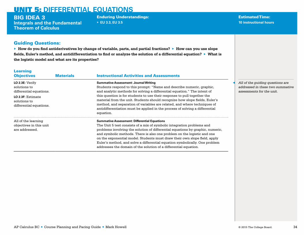
AP Calculus BC ■ Course Planning and Pacing Guide ■ Mark Howell © 2015 The College Board. 34
UNIT 1: LIMITS AND CONTINUITYBIG IDEA 1 Limits
Enduring Understandings:▶▶ EU 1.1, EU 1.2
Estimated Time:15 Hours
Guiding Questions:▶ How do you find antiderivatives by change of variable, parts, and partial fractions? ▶ How can you use slope fields, Euler’s method, and antidifferentiation to find or analyze the solution of a differential equation? ▶ What is the logistic model and what are its properties?
Learning Objectives Materials Instructional Activities and Assessments
LO 2.3E: Verify solutions to differential equations.
LO 2.3F: Estimate solutions to differential equations.
Summative Assessment: Journal WritingStudents respond to this prompt: “Name and describe numeric, graphic, and analytic methods for solving a differential equation.” The intent of this question is for students to use their response to pull together the material from the unit. Students should recognize how slope fields, Euler’s method, and separation of variables are related, and where techniques of antidifferentiation must be applied in the process of solving a differential equation.
◀ All of the guiding questions are addressed in these two summative assessments for the unit.
All of the learning objectives in this unit are addressed.
Summative Assessment: Differential EquationsThe Unit 5 test consists of a mix of symbolic integration problems and problems involving the solution of differential equations by graphic, numeric, and symbolic methods. There is also one problem on the logistic and one on the exponential model. Students must draw their own slope field, apply Euler’s method, and solve a differential equation symbolically. One problem addresses the domain of the solution of a differential equation.
UNIT 5: DIFFERENTIAL EQUATIONSBIG IDEA 3 Integrals and the Fundamental Theorem of Calculus
Enduring Understandings:▶▶ EU 3.3, EU 3.5
Estimated Time:10 instructional hours

AP Calculus BC ■ Course Planning and Pacing Guide ■ Mark Howell © 2015 The College Board. 35
The following activities and techniques in Unit 5 help students learn to apply the Mathematical Practices for AP Calculus (MPACs):
MPAC 2 — Connecting concepts: The instructional activity on Euler’s method links the ideas of local linearity and tangent lines to the iterative process of Euler’s method.
MPAC 3 — Implementing algebraic/computational processes: Several activities in this unit involve the practice of carrying out computational processes, including the formative assessment “Finding Antiderivatives”; the instructional activity on Euler’s method, which also incorporates technology to solve a problem; and the unit test, where students complete the process of finding the solution of a differential equation symbolically.
MPAC 4 — Connecting multiple representations: The instructional activity “Multiple Representational Approach to Solving Differential Equations” explicitly connects three ways of looking at the solution of a differential equation. The formative assessment at the end of the unit asks students to write about these three representations in their journals.
MPAC 5 — Building notational fluency: The symbolic process of solving a differential equation could serve as the poster child for notational fluency! Students select, carry out, and interpret a symbolic process when they find a function containing an initial condition and having a certain derivative. In the summative unit test, students solve such problems when the derivative is presented using different notations. The problems contained in the formative assessment on finding antiderivatives are posed using a variety of notations. For example, all of these types of prompts appear:
▶▶ What is ?
▶▶ If , what is ?
▶▶ Find a function whose derivative is given by .
▶▶ What is an antiderivative for ?
MPAC 6 — Communicating: In response to a journal prompt, students describe how finding the equation of a line with a certain slope and containing a certain point is the same as finding a function with a certain derivative and containing an initial condition.
The summative assessment at the end of this unit addresses all of the MPACs.
UNIT 5: DIFFERENTIAL EQUATIONS
Mathematical Practices for AP Calculus in Unit 5

AP Calculus BC ■ Course Planning and Pacing Guide ■ Mark Howell © 2015 The College Board. 36
Guiding Questions:▶ How can the definite integral be used to find the net or total change of a quantity whose rate of change is known? ▶ What is the connection between the Fundamental Theorem of Calculus and applications of the integral? ▶ How do you use the definite integral to find area, volume, and arc length?
Learning Objectives Materials Instructional Activities and Assessments
LO 3.4D: Apply definite integrals to problems involving area, volume, (BC) and length of a curve.
LO 3.4B: Apply definite integrals to problems involving the average value of a function.
Print Finney et al., chapter 8
Instructional Activity: Area of a RegionI emphasize that the area of any region can be found by evaluating
where is the “top” curve and is the “bottom” curve. Similarly, when integrating with respect to y to find the area of a
region, we evaluate where is the “right-most” curve
and is the “left-most” curve.
◀ We revisit the idea of average value, first presented briefly in Unit 4, in the context of area. The idea of multiplying the average value of the function by the width of the interval, , to get the area under the graph of a positive function, is a natural way to view the average value formula. That
is, gives
the area under the graph of f,
i.e. .
LO 3.4D: Apply definite integrals to problems involving area, volume, (BC) and length of a curve.
LO 3.4B: Apply definite integrals to problems involving the average value of a function.
Print Finney et al., chapter 8
Instructional Activity: Archimedes’s Formula for the Area of a Parabolic Region A homework problem gives rise to a conjecture that the area inside a parabolic region centered at the vertex is two-thirds of the area of the circumscribed rectangle. We prove this result for a general parabolic region in a teacher-guided discussion. The region under the graph of from
to is calculated using , and compared with the area
of the rectangle with vertices , and , which is .
UNIT 6: APPLICATIONS OF THE DEFINITE INTEGRALBIG IDEA 3 Integrals and the Fundamental Theorem of Calculus
Enduring Understandings:▶▶ EU 3.4
Estimated Time:9 instructional hours

AP Calculus BC ■ Course Planning and Pacing Guide ■ Mark Howell © 2015 The College Board. 37
Guiding Questions:▶ How can the definite integral be used to find the net or total change of a quantity whose rate of change is known? ▶ What is the connection between the Fundamental Theorem of Calculus and applications of the integral? ▶ How do you use the definite integral to find area, volume, and arc length?
Learning Objectives Materials Instructional Activities and Assessments
LO 3.4D: Apply definite integrals to problems involving area, volume, (BC) and length of a curve.
LO 3.4B: Apply definite integrals to problems involving the average value of a function.
Print Finney et al., chapter 8
Instructional Activity: Volume of a Solid with Known Cross-Sectional AreaEvery volume problem in AP Calculus can be solved using either
or where or is the area of a general
cross section of the solid. I emphasize that when the solid is formed by revolving a region around a horizontal or vertical line, the cross section is either a circle or a “washer.” So the cross-sectional area is given by a formula like , where R and r are the radii of the outer and inner circles, respectively. Students solve problems using this general approach.
LO 3.4A: Interpret the meaning of a definite integral within a problem.
LO 3.4C: Apply definite integrals to problems involving motion.
LO 3.4E: Use the definite integral to solve problems in various contexts.
Print Finney et al., chapter 8
Instructional Activity: Integral as Net ChangePrevious work with the Car Lab and the Fundamental Theorem serves as the conceptual underpinning for this activity. Students saw that the integral of the rate of change of position (i.e., velocity) yielded the net change in position. Change the word “position” to any other quantity, and the same result holds. See the Thought Box below on “Formative Assessment: Journal Writing.” Students set up and evaluate definite integrals in order to determine the net change in a quantity whose rate of change is known.
UNIT 6: APPLICATIONS OF THE DEFINITE INTEGRALBIG IDEA 3 Integrals and the Fundamental Theorem of Calculus
Enduring Understandings:▶▶ EU 3.4
Estimated Time:9 instructional hours

AP Calculus BC ■ Course Planning and Pacing Guide ■ Mark Howell © 2015 The College Board. 38
UNIT 1: LIMITS AND CONTINUITYBIG IDEA 1 Limits
Enduring Understandings:▶▶ EU 1.1, EU 1.2
Estimated Time:15 Hours
Guiding Questions:▶ How can the definite integral be used to find the net or total change of a quantity whose rate of change is known? ▶ What is the connection between the Fundamental Theorem of Calculus and applications of the integral? ▶ How do you use the definite integral to find area, volume, and arc length?
Learning Objectives Materials Instructional Activities and Assessments
LO 3.4E: Use the definite integral to solve problems in various contexts.
Formative Assessment: Journal WritingStudents respond to this prompt: “Think of one real-world setting where some quantity changes at a variable rate. What would you need to know to determine how much the quantity changes over some time period? How would you find how much the quantity changes?” Students discuss their responses to this prompt in class.
◀ Some students need additional guidance in responding to this prompt. Recalling the Fundamental Theorem, I refer them to the equation
. The
function f represents a quantity whose rate of change is known. In fact, it is known as . The quantity represents the net change in f from to .
LO 3.4D: Apply definite integrals to problems involving area, volume, (BC) and length of a curve.
Instructional Activity: Volume of a SolidI emphasize that all volume problems are solved using the same formula:
, where is the cross-sectional area of the solid that extends
from to . If that solid is one formed by revolving a region around an axis, then is either the area of a circle or a “washer.” Otherwise,
must either be directly given or described geometrically.
All of the learning objectives in this unit are addressed.
Summative Assessment: Applications of the IntegralFor the Unit 6 test, I try to assess all of the applications of the integral students have seen. For grading, more emphasis is given to setting up integrals, rather than evaluating them. Usually, this test is all open calculator. Problems on area, volume, arc length, particle motion, and a real world context problem involving the integral of a rate of change to calculate net change all appear on the test.
◀ This summative assessment addresses all of the guiding questions for the unit.
UNIT 6: APPLICATIONS OF THE DEFINITE INTEGRALBIG IDEA 3 Integrals and the Fundamental Theorem of Calculus
Enduring Understandings:▶▶ EU 3.4
Estimated Time:9 instructional hours

AP Calculus BC ■ Course Planning and Pacing Guide ■ Mark Howell © 2015 The College Board. 39
The following activities and techniques in Unit 6 help students learn to apply the Mathematical Practices for AP Calculus (MPACs):
MPAC 1 — Reasoning with definitions and theorems: In the instructional activity “Volume of a Solid with Known Cross-Sectional Area,” I emphasize to students that the same formula, , is used for all volume problems. Solids of revolution are treated the same as other solids with known cross-sectional area.
MPAC 2 — Connecting concepts: The definition of the integral involves the limit of the sum of products. The factors in the product are always the dependent variable (function output) and independent variable (function input). Recognizing this simple fact helps students understand the meaning of the integral in context by focusing on the units attached to these two quantities.
MPAC 3 — Implementing algebraic/computational processes: Students must implement multistep analytic and algebraic procedures to determine the correct integrand for area and volume problems.
MPAC 4 — Connecting multiple representations: The instructional activity “Integral as Net Change” emphasizes the connection between a verbal description of how the integral is applied to real-world contexts and the symbolic statement of the Fundamental Theorem of Calculus.
MPAC 5 — Building notational fluency: Throughout the unit, students set up definite integrals to answer questions about area, volume, distance traveled, arc length, and so on. All of these exercises help to familiarize students with the notation and meaning of the definite integral.
MPAC 6 — Communicating: In the summative assessment, students must interpret the meaning of a definite integral in context, using correct units.
UNIT 6: APPLICATIONS OF THE DEFINITE INTEGRAL
Mathematical Practices for AP Calculus in Unit 6

AP Calculus BC ■ Course Planning and Pacing Guide ■ Mark Howell © 2015 The College Board. 40
Guiding Questions:▶ How is the idea of limits extended to include limits of sequences? ▶ What are indeterminate forms, and how can L’Hospital’s Rule be applied to evaluate limits and to determine when one function grows faster than another? ▶ How do you use limits to evaluate the two types of improper integrals?
Learning Objectives Materials Instructional Activities and Assessments
LO 1.1A(a): Express limits symbolically using correct notation.
LO 1.1A(b): Interpret limits expressed symbolically.
LO 1.1B: Estimate limits of functions.
LO 1.1C: Determine limits of functions.
Print Finney et al., chapter 9
Web“A Local Linearity Approach to Calculus”
Instructional Activity: Limits of Sequences and L’Hospital’s RuleA sequence is a function whose domain is a subset of the natural numbers. Though sequences are not explicitly tested on the AP Calculus BC Exam, convergence of infinite series is defined in terms of the limit of a sequence of partial sums, so it is important to cover sequences. This activity also serves as a good review of properties of limits. The rationale for L’Hospital’s Rule (section 9.2 in Finney et al.) is another opportunity to connect local linearity with important calculus results. Students evaluate the limit of several sequences, including the sequence of partial sums of the geometric
series for various values of r, and the sequence , which
diverges because of the oscillations.
LO 1.1C: Determine limits of functions.
Print Finney et al., chapter 9
Web“A Local Linearity Approach to Calculus”
Formative Assessment: Journal WritingStudents respond to this prompt in their journal: “How does local linearity help explain L’Hospital’s Rule?” Even though we have discussed the connection in class, I believe that writing about their understanding of this connection will cement the concept for students. When students have trouble getting started, I refer them to page three of “A Local Linearity Approach to Calculus,” which has a good explanation of how L’Hospital’s Rule can be understood through the lens of local linearity.
◀ When students struggle with the rationale behind L’Hospital’s Rule, we use computer software to zoom in to the graph of two functions with a common x-intercept, and show the ratio of the slopes on the graphs as they straighten out.
UNIT 7: SEQUENCES, L’HOSPITAL’S RULE, AND IMPROPER INTEGRALSBIG IDEA 1 Limits BIG IDEA 3 Integrals and the Fundamental Theorem of Calculus
Enduring Understandings:▶▶ EU 1.1, EU 3.2
Estimated Time:8 instructional hours

AP Calculus BC ■ Course Planning and Pacing Guide ■ Mark Howell © 2015 The College Board. 41
Guiding Questions:▶ How is the idea of limits extended to include limits of sequences? ▶ What are indeterminate forms, and how can L’Hospital’s Rule be applied to evaluate limits and to determine when one function grows faster than another? ▶ How do you use limits to evaluate the two types of improper integrals?
Learning Objectives Materials Instructional Activities and Assessments
LO 1.1D: Deduce and interpret behavior of functions using limits.
Print Finney et al., chapter 9
Web“A Local Linearity Approach to Calculus”
Instructional Activity: Relative Growth RatesI like to motivate this topic with this question from precalculus, posed to the entire class: “How may points of intersection do the graphs of and
have?” Looking at the graphs in a standard viewing window would lead students to assume that there are two points of intersection. However, since exponential growth “beats” polynomial growth, eventually, the graph of “catches up” to the graph of , and there is a third point of intersection.
LO 1.1D: Deduce and interpret behavior of functions using limits.
Print Finney et al., chapter 9
Web“A Local Linearity Approach to Calculus”
Formative Assessment: Journal WritingStudents respond to this prompt: “Explain why logarithms grow slower than polynomials, and why polynomials grow slower than exponential functions with a base greater than 1.” Students discuss their responses to this prompt in class.
◀ A class discussion of journal answers initiates an explanation involving L’Hospital’s rule, applied
to evaluate , where P
is a polynomial function, or to
evaluate , where .
LO 3.2D: (BC) Evaluate an improper integral or show that an improper integral diverges.
Print Finney et al., chapter 9
Web“A Local Linearity Approach to Calculus”
Instructional Activity: Improper IntegralsMy strategy here is similar to the one I use in covering related rates problems. Students combine their understanding of limits with the Fundamental Theorem to figure out whether an improper integral converges, and if it does, what it converges to. We discuss the two types of improper integrals as “horizontal” (where a limit of integration is infinite) or “vertical” (where the integrand grows without bound).
UNIT 7: SEQUENCES, L’HOSPITAL’S RULE, AND IMPROPER INTEGRALSBIG IDEA 1 Limits BIG IDEA 3 Integrals and the Fundamental Theorem of Calculus
Enduring Understandings:▶▶ EU 1.1, EU 3.2
Estimated Time:8 instructional hours

AP Calculus BC ■ Course Planning and Pacing Guide ■ Mark Howell © 2015 The College Board. 42
UNIT 7: SEQUENCES, L’HOSPITAL’S RULE, AND IMPROPER INTEGRALSBIG IDEA 1 Limits BIG IDEA 3 Integrals and the Fundamental Theorem of Calculus
Enduring Understandings:▶▶ EU 1.1, EU 3.2
Estimated Time:8 instructional hours
Guiding Questions:▶ How is the idea of limits extended to include limits of sequences? ▶ What are indeterminate forms, and how can L’Hospital’s Rule be applied to evaluate limits and to determine when one function grows faster than another? ▶ How do you use limits to evaluate the two types of improper integrals?
Learning Objectives Materials Instructional Activities and Assessments
All of the learning objectives in this unit are addressed.
Summative Assessment: Sequences, L’Hospital’s Rule, and Improper Integrals This unit test is challenging for students. It includes some nonstandard
questions, like this one: “Determine a and b so that .”
Students need to recognize the need for an indeterminate form at the outset. There are limit problems involving all the different indeterminate forms that can be answered with L’Hospital’s Rule, as well as several improper integrals to evaluate. One problem asks this: “A student does the following
on a homework problem: . Explain exactly
what error the student, who is otherwise a good person, made.” Another asks students to rank 10 functions in order from slowest to fastest growing.
◀ This summative assessment addresses all of the guiding questions for the unit.

AP Calculus BC ■ Course Planning and Pacing Guide ■ Mark Howell © 2015 The College Board. 43
The following activities and techniques in Unit 7 help students learn to apply the Mathematical Practices for AP Calculus (MPACs):
MPAC 1 — Reasoning with definitions and theorems: Applying L’Hospital’s Rule requires students to check that the hypotheses of a theorem are met. Examples are given in the instructional activity “Limits of Sequences and L’Hospital’s Rule” where a lack of attention to that detail results in errors. The instructional activity on improper integrals requires students to pay close attention to when an improper integral is said to converge based on a definition.
MPAC 2 — Connecting concepts: The instructional activity “Improper Integrals” combines two Big Ideas: limits and integrals. The instructional activity “Relative Growth Rates” connects the limit of the ratio of two functions with their growth rates. We investigate this both graphically and numerically.
MPAC 3 — Implementing algebraic/computational processes: Problems involving analyzing and evaluating improper integrals require students to carry out a computational process that takes several steps: identifying what limit to evaluate; constructing the combination of a limit with an integral; evaluating the integral in terms of a limit of integration; and finally, taking the limit of the result.
MPAC 4 — Connecting multiple representations: Both the first instructional activity of the unit and the ensuing journal question use the connection between the graphic, numeric, and symbolic representations of two functions and their derivatives.
MPAC 5 — Building notational fluency: When evaluating improper integrals, students combine the notation for taking the limit with that of a definite integral. In particular, they must be careful to apply the Fundamental Theorem with limits of integration that are real numbers. So I emphasize the importance of communicating mathematics
correctly by writing .
MPAC 6 — Communicating: In the summative assessment, students must explain the error in misapplying the Fundamental Theorem to evaluate an integral, in a case where the integrand has a discontinuity.
UNIT 7: SEQUENCES, L’HOSPITAL’S RULE, AND IMPROPER INTEGRALS
Mathematical Practices for AP Calculus in Unit 7

AP Calculus BC ■ Course Planning and Pacing Guide ■ Mark Howell © 2015 The College Board. 44
Guiding Questions:▶ How do you define convergence and divergence of an infinite series, and how can the definition be applied to analyze some common convergent and divergent infinite series? ▶ How can you test when an infinite series converges, and how do these tests make sense? ▶ How are Taylor polynomials used to approximate functions? ▶ What is a Taylor series and what are the consequences of Taylor’s theorem?
Learning Objectives Materials Instructional Activities and Assessments
LO 4.1A: Determine whether a series converges or diverges.
LO 4.1B: Determine or estimate the sum of a series.
Print Finney et al., chapter 10
Instructional Activity: Repeating Decimals as Infinite Geometric SeriesI begin our coverage of infinite series by presenting students with some comfortable examples, hoping to improve self-confidence as we begin this daunting topic. We investigate repeating decimals, such as 0.333 … , and notice two important facts: the repeating decimal is actually an infinite geometric series, 3/10 + 3/100 + 3/1000 + … ; and the series converges to one-third. We define convergence of an infinite series as the existence of the limit of the sequence of partial sums, and apply that definition to a couple of
series that do not converge: and .
◀ This activity addresses the first guiding question. Students participate in the development of the definition of convergence, and see how to apply that definition to these simple examples.
LO 4.1A: Determine whether a series converges or diverges.
LO 4.1B: Determine or estimate the sum of a series.
SoftwareANHARM calculator program for demonstration purposes
Instructional Activity: The Harmonic and the Alternating Harmonic SeriesThis activity is teacher guided and takes the form of a conversation with the class. I use a calculator program to display the sequence of partial sums for
the harmonic and alternating harmonic series and .
After 20 minutes, it seems clear that the latter series converges. Students are divided in their opinions about the convergence of the harmonic series. That motivates us to consider ways to test for convergence. An argument
approximating with a left-hand Riemann sum and rectangles of
width 1 (the sum of which is exactly the harmonic series) convinces the
skeptics that the harmonic series indeed diverges. An argument that examines partial sums convinces students that the alternating harmonic series converges.
◀ The justifications we do here serve as a nice introduction to two important tests for convergence: the integral test, which is essentially a generalization of the argument for the divergence of the harmonic series, and the alternating series test (with error bound), which is a generalization of the argument for the convergence of the alternating harmonic series.
UNIT 8: SERIESBIG IDEA 4 Series (BC)
Enduring Understandings:▶▶ EU 4.1, EU 4.2
Estimated Time:17 instructional hours

AP Calculus BC ■ Course Planning and Pacing Guide ■ Mark Howell © 2015 The College Board. 45
Guiding Questions:▶ How do you define convergence and divergence of an infinite series, and how can the definition be applied to analyze some common convergent and divergent infinite series? ▶ How can you test when an infinite series converges, and how do these tests make sense? ▶ How are Taylor polynomials used to approximate functions? ▶ What is a Taylor series and what are the consequences of Taylor’s theorem?
Learning Objectives Materials Instructional Activities and Assessments
LO 4.2B: Write a power series representing a given function.
LO 4.2C: Determine the radius and interval of convergence of a power series.
Print Finney et al., chapter 10
WebCollege Board Special Focus materials on series
“Setting the Stage with Geometric Series”
Instructional Activity: Interval of Convergence Students work individually to graph the following functions on the
same screen: , , , and so on, up to
. After noticing that these functions represent a sequence of partial sums for the infinite geometric series with common
ratio x, we graph on top of all of them, and notice that the functions
converge to a long as x is between –1 and 1. This introduces the
idea of an interval of convergence.
UNIT 8: SERIESBIG IDEA 4 Series (BC)
Enduring Understandings:▶▶ EU 4.1, EU 4.2
Estimated Time:17 instructional hours

AP Calculus BC ■ Course Planning and Pacing Guide ■ Mark Howell © 2015 The College Board. 46
Guiding Questions:▶ How do you define convergence and divergence of an infinite series, and how can the definition be applied to analyze some common convergent and divergent infinite series? ▶ How can you test when an infinite series converges, and how do these tests make sense? ▶ How are Taylor polynomials used to approximate functions? ▶ What is a Taylor series and what are the consequences of Taylor’s theorem?
Learning Objectives Materials Instructional Activities and Assessments
LO 4.2B: Write a power series representing a given function.
LO 4.2C: Determine the radius and interval of convergence of a power series.
Print Finney et al., chapter 10
WebCollege Board Special Focus materials on series
“Setting the Stage with Geometric Series”
Instructional Activity: From the Geometric Series to the Series for the Arctangent FunctionI use this activity to introduce the idea of creating new series from old by substitution and integration. It has the added benefit of being most captivating! Here’s the process. I guide students through the activity, but each student writes out the details.
1. (geometric series)
Replace by :
2.
Replace by :
3.
Antidifferentiate termwise:
4.
Substitute , and we get a series that converges to . Cool! Go back
to the series at step 2, and antidifferentiate termwise:
5.
Substitute , and we get the alternating harmonic series converging to. The earlier calculator-produced number, about 0.693, is revealed.
Note that this procedure uses a theorem that guarantees that the radius of convergence is unchanged when we antidifferentiate termwise.
◀ I think this activity is powerful, mysterious, and illuminating all at the same time! For students to participate in a process that yields a series that can be used to approximate pi and another that approximates is mathematically enriching.
UNIT 8: SERIESBIG IDEA 4 Series (BC)
Enduring Understandings:▶▶ EU 4.1, EU 4.2
Estimated Time:17 instructional hours

AP Calculus BC ■ Course Planning and Pacing Guide ■ Mark Howell © 2015 The College Board. 47
Guiding Questions:▶ How do you define convergence and divergence of an infinite series, and how can the definition be applied to analyze some common convergent and divergent infinite series? ▶ How can you test when an infinite series converges, and how do these tests make sense? ▶ How are Taylor polynomials used to approximate functions? ▶ What is a Taylor series and what are the consequences of Taylor’s theorem?
Learning Objectives Materials Instructional Activities and Assessments
LO 4.2A: Construct and use Taylor polynomials.
LO 4.2B: Write a power series representing a given function.
PrintHughes-Hallett et al. AP Guide for Calculus: Single Variable, Lab 10
Instructional Activity: A Numeric Investigation into the Accuracy of Polynomial Approximations to Transcendental FunctionsThis calculator activity leads students to discover the coefficients of special
second- and third-degree polynomials that approximate near . By looking at the limit of the error relative to in using the tangent line to
approximate , that is, , students empirically determine that
if they add to the tangent line, the error relative to will approach 0
(a good thing!). That is, . In a similar way, we then
determine a cubic polynomial approximation whose error relative to
approaches 0 as approaches 0. That is, . Cool!
◀ This is another one of my favorite activities. As a follow-up, it is a simple matter to verify that the output and first three derivatives of the cubic polynomial approximation for at are the same as the output and first three derivatives for . That is, we have discovered the third-degree Taylor polynomial. Awesome.
UNIT 8: SERIESBIG IDEA 4 Series (BC)
Enduring Understandings:▶▶ EU 4.1, EU 4.2
Estimated Time:17 instructional hours

AP Calculus BC ■ Course Planning and Pacing Guide ■ Mark Howell © 2015 The College Board. 48
UNIT 1: LIMITS AND CONTINUITYBIG IDEA 1 Limits
Enduring Understandings:▶▶ EU 1.1, EU 1.2
Estimated Time:15 Hours
Guiding Questions:▶ How do you define convergence and divergence of an infinite series, and how can the definition be applied to analyze some common convergent and divergent infinite series? ▶ How can you test when an infinite series converges, and how do these tests make sense? ▶ How are Taylor polynomials used to approximate functions? ▶ What is a Taylor series and what are the consequences of Taylor’s theorem?
Learning Objectives Materials Instructional Activities and Assessments
LO 4.2B: Write a power series representing a given function.
Print Finney et al., chapter 10
Instructional Activity: Working with Taylor Series
Once we cover the Taylor series for , , and , we do a teacher-guided lesson involving connections among these series. For example, differentiating both sides of the equation
yields the series for the cosine. I
point out that the powers of all the terms in the series for sine are odd, and the sine is an odd function. A similar result follows with the even powers in
the series for cosine. Differentiate both sides of the series for and you get the same series back! And there’s a cool way to showcase Euler’s identity,
, using series.
LO 4.2A: Construct and use Taylor polynomials.
Print Finney et al., chapter 10
Instructional Activity: Lagrange Error Bound and Taylor’s TheoremIn this activity, we find the c promised by Taylor’s theorem for the Maclaurin polynomial with and , and graph the third-degree Taylor
polynomial, with . Using x = , we find the c in the interval
(0, ), and illustrate the quantity as the length of a vertical line
segment connecting the graphs.
◀ I think this is the toughest topic in AP Calculus, and it takes at least a couple of days to cover in depth. I’ve found it especially helpful to look at Taylor’s theorem for the case where . Students see that this is exactly the Mean Value Theorem!
UNIT 8: SERIESBIG IDEA 4 Series (BC)
Enduring Understandings:▶▶ EU 4.1, EU 4.2
Estimated Time:17 instructional hours

AP Calculus BC ■ Course Planning and Pacing Guide ■ Mark Howell © 2015 The College Board. 49
Guiding Questions:▶ How do you define convergence and divergence of an infinite series, and how can the definition be applied to analyze some common convergent and divergent infinite series? ▶ How can you test when an infinite series converges, and how do these tests make sense? ▶ How are Taylor polynomials used to approximate functions? ▶ What is a Taylor series and what are the consequences of Taylor’s theorem?
Learning Objectives Materials Instructional Activities and Assessments
LO 4.1A: Determine whether a series converges or diverges.
LO 4.1B: Determine or estimate the sum of a series.
LO 4.2A: Construct and use Taylor polynomials.
Formative Assessment: Journal Writing
Students respond to this journal prompt: “Can the value of be
calculated with an accuracy of using only addition, subtraction,
multiplication, and division? Explain your answer. If this is possible, how many terms must be added (or subtracted)?”
◀ This question gets at the heart of one of the theoretical applications of Taylor series, and the alternating series error bound. As with all of the journal writing exercises, students’ responses serve to initiate a class discussion that can resolve any misconceptions.
LO 4.2A: Construct and use Taylor polynomials.
LO 4.2C: Determine the radius and interval of convergence of a power series.
Web“Taylor Polynomial Approximation”
Instructional Activity: Geogebra Investigation into Taylor Polynomials and ErrorThis short teacher-guided spectacle uses a Geogebra applet that displays Taylor polynomials. A control allows the user to change the degree dynamically. You can observe the behavior of the graph of the error function (i.e., the difference between the Taylor polynomial and the function it approximates).
LO 4.1A: Determine whether a series converges or diverges.
Web College Board Special Focus materials on series
“Overview of Tests for Convergence of Infinite Series”
Instructional Activity: Tests for ConvergenceMost of the core ideas that lead to the tests of convergence are covered “on the side” during the various instructional activities of the unit. The integral test and the alternating series test, for example, come up in the activity involving the harmonic and alternating harmonic series. Here, all the tests are covered at one time. The limit comparison test and the ratio test get special attention since they were not touched on earlier. The former is not covered in the Special Focus materials.
UNIT 8: SERIESBIG IDEA 4 Series (BC)
Enduring Understandings:▶▶ EU 4.1, EU 4.2
Estimated Time:17 instructional hours

AP Calculus BC ■ Course Planning and Pacing Guide ■ Mark Howell © 2015 The College Board. 50
Guiding Questions:▶ How do you define convergence and divergence of an infinite series, and how can the definition be applied to analyze some common convergent and divergent infinite series? ▶ How can you test when an infinite series converges, and how do these tests make sense? ▶ How are Taylor polynomials used to approximate functions? ▶ What is a Taylor series and what are the consequences of Taylor’s theorem?
Learning Objectives Materials Instructional Activities and Assessments
LO 4.1A: Determine whether a series converges or diverges.
LO 4.1B: Determine or estimate the sum of a series.
LO 4.2A: Construct and use Taylor polynomials.
LO 4.2B: Write a power series representing a given function.
LO 4.2C: Determine the radius and interval of convergence of a power series.
Summative Assessment: SeriesThe unit test includes the following problem types:
1. Use a Taylor polynomial of a specified degree to approximate a function output. For example,
2. A set of always, sometimes, never questions. This format allows testing of
simple, fundamental concepts. One of these is If , then .
3. Find a new series from an old one by substitution.
4. Find the interval of convergence for a power series.
5. Apply a specified test to determine whether or not a series converges. There’s one question for each test in the course.
6. Find a new series from an old one by antidifferentiation.
In addition to these, there’s a question on the alternating series error bound and on the Lagrange error bound.
◀ This summative assessment addresses all of the guiding questions for the unit.
UNIT 8: SERIESBIG IDEA 4 Series (BC)
Enduring Understandings:▶▶ EU 4.1, EU 4.2
Estimated Time:17 instructional hours

AP Calculus BC ■ Course Planning and Pacing Guide ■ Mark Howell © 2015 The College Board. 51
The following activities and techniques in Unit 8 help students learn to apply the Mathematical Practices for AP Calculus (MPACs):
MPAC 1 — Reasoning with definitions and theorems: A key result of the instructional activity “Repeating Decimals as Infinite Geometric Series” is the definition of convergence of an infinite series as the existence of the limit of the sequence of partial sums. Students apply this definition to make conclusions about the convergence of several series.
MPAC 2 — Connecting concepts: The instructional activity “Interval of Convergence” connects the concept of an interval of convergence with its graphical representation.
MPAC 3 — Implementing algebraic/computational processes: In order to determine an interval of convergence using the ratio test and other convergence tests, students must apply a procedure involving limits, testing endpoints, and putting together an interval. Students follow a computational process when forming a Taylor polynomial.
MPAC 4 — Connecting multiple representations: Two activities in this unit use graphical representations to illustrate important concepts about power series. The instructional activity “Interval of Convergence” uses graphs to introduce the idea of the interval of convergence for a power series. Later, the instructional activity “Geogebra Investigation into Taylor Polynomials and Error” offers a dramatic graphic view of Taylor polynomials converging to the function they are approximating with increasing degree.
MPAC 5 — Building notational fluency: Students work extensively with summation notation, limits, integrals, and derivatives throughout this unit.
MPAC 6 — Communicating: When students respond to the journal question about calculating the value of using only addition, subtraction, multiplication, and division in the formative assessment, they must explain their answer. A problem on the summative assessment requires students to justify their answer using the alternating series error bound.
UNIT 8: SERIES
Mathematical Practices for AP Calculus in Unit 8

AP Calculus BC ■ Course Planning and Pacing Guide ■ Mark Howell © 2015 The College Board. 52
Guiding Questions:▶ How does what we know about derivatives apply to parametric and polar curves? ▶ How do you use the integral to find the length of parametric and polar curves? ▶ How do you use the integral to find the area of a region bounded by one or more polar curves?
Learning Objectives Materials Instructional Activities and Assessments
LO 2.1C: Calculate derivatives.
LO 2.2A: Use derivatives to analyze properties of a function.
PrintFinney et al., chapter 11
Instructional Activity: Derivatives of Parametric and Polar FunctionsRather than asking students to memorize formulas, I approach this unit as a simple application of the chain rule to calculate slopes of parametric and polar curves. We calculate the slope of the polar curve at the Cartesian point three ways: by writing a Cartesian form of the
curve and using implicit differentiation; by parameterizing
the curve using , , and using , after finding
the angle t that gives the point ; and by using the polar to rectangular
conversions to write , , then using
, after calculating the angle for the point .
◀ I spend 10 hours on this unit, but it can be covered in much less time than that. We take three semesters for the AP Calculus BC course, so can afford more time on polar and parametric functions. Seven hours is probably adequate for a two-semester course.
LO 2.1C: Calculate derivatives.
LO 2.3C: Solve problems involving related rates, optimization, rectilinear motion, (BC) and planar motion.
LO 3.4C: Apply definite integrals to problems involving motion.
PrintFinney et al., chapter 11
Instructional Activity: Motion in the PlaneDuring this activity, students use the parametric plotting feature of the
calculator to display the motion of a particle along a line. Set and, for , with a t step of 0.2 and define a suitable viewing
window. Then trace on the graph to see the particle move on a line. Students determine the position, velocity, and acceleration at integer times, and connect the results to the motion. The next day, we start with a velocity function and an initial position, and use it to determine net and total distance traveled over the time interval from 0 to 5.
◀ I cover vectors and parametric functions together. It’s natural to use two parametric functions, one for the horizontal and one for the vertical component, to represent position, velocity, and acceleration vectors in the plane.
UNIT 9: PARAMETRIC AND POLAR FUNCTIONSBIG IDEA 2 Derivatives BIG IDEA 3 Integrals and the Fundamental Theorem of Calculus
Enduring Understandings:▶▶ EU 2.1, EU 2.2, EU 3.4
Estimated Time:7 instructional hours

AP Calculus BC ■ Course Planning and Pacing Guide ■ Mark Howell © 2015 The College Board. 53
Guiding Questions:▶ How does what we know about derivatives apply to parametric and polar curves? ▶ How do you use the integral to find the length of parametric and polar curves? ▶ How do you use the integral to find the area of a region bounded by one or more polar curves?
Learning Objectives Materials Instructional Activities and Assessments
LO 3.4D: Apply definite integrals to problems involving area, volume, (BC) and length of a curve.
PrintFinney et al., section 11.3, problem 60
Instructional Activity: Area of a Polar RegionThe difference between finding the area of a region in the Cartesian plane and the area of a polar region is that instead of adding the areas of thin rectangles, we’re adding the areas of circular sectors. It’s compelling to calculate the area of a region two ways: by using the polar methodology, and by using the rectangular methodology. We find the area of the region
bounded by the x-axis and the graphs of and by evaluating
. We show that the same region is bounded by the
graph of with from 0 to . So we evaluate
, and get the same answer.
LO 3.4D: Apply definite integrals to problems involving area, volume, (BC) and length of a curve.
Formative Assessment: Journal WritingStudents respond to this prompt in their journal: “Explain why the word ‘smooth’ appears in the section titled ‘Length of a Smooth Curve’.” If a function fails to be differentiable at a point in the interval over which you’re calculating the length of its graph, the arc length formula doesn’t apply. So, some caution is needed when using the formula. Occasionally, you can split the curve into two pieces to find the length. If the lack of differentiability results from a vertical tangent, you can sometimes interchange the variable to transform the vertical tangent to a horizontal one.
◀ I usually give an arc length problem with a point of nondifferentiability on a follow-up quiz after this journal assignment. If it seems that the lesson wasn’t learned, I ask students to find the length of the graph of from 1 to 1. If they mindlessly enter the integral into their calculator without checking the behavior at , the calculator barks at them.
UNIT 9: PARAMETRIC AND POLAR FUNCTIONSBIG IDEA 2 Derivatives BIG IDEA 3 Integrals and the Fundamental Theorem of Calculus
Enduring Understandings:▶▶ EU 2.1, EU 2.2, EU 3.4
Estimated Time:7 instructional hours

AP Calculus BC ■ Course Planning and Pacing Guide ■ Mark Howell © 2015 The College Board. 54
Guiding Questions:▶ How does what we know about derivatives apply to parametric and polar curves? ▶ How do you use the integral to find the length of parametric and polar curves? ▶ How do you use the integral to find the area of a region bounded by one or more polar curves?
Learning Objectives Materials Instructional Activities and Assessments
LO 3.4D: Apply definite integrals to problems involving area, volume, (BC) and length of a curve.
PrintFinney et al., chapter 11
Instructional Activity: Length of a CurveStudents first see arc length problems in Chapter 8. They are revisited here in the context of parametric functions. We do an exploration that investigates the length of one arch of the cycloid parameterized by
, with . As in Chapter 8, I’m more concerned that students can set up an integral that gives the length. Evaluating such integrals is generally better relegated to a machine at this point.
All of the learning objectives in this unit are addressed.
Summative Assessment: Parametric and Polar FunctionsThe Unit 9 test has at least one question for each of the major calculus applications involving polar and vector functions. Students find the length of a polar curve and the area of a region bounded by the graphs of two polar curves. Given the x and y components of the velocity vector of a particle moving in the plane, students find a tangent line, the speed and acceleration vector at a certain time, and the total distance traveled. In a closed calculator part, students calculate the slope of a polar curve, and determine where the graph of a parametrically defined curve is concave up. Another closed calculator problem asks for the length of a parametrically defined curve.
◀ This summative assessment addresses all of the guiding questions for the unit.
UNIT 9: PARAMETRIC AND POLAR FUNCTIONSBIG IDEA 2 Derivatives BIG IDEA 3 Integrals and the Fundamental Theorem of Calculus
Enduring Understandings:▶▶ EU 2.1, EU 2.2, EU 3.4
Estimated Time:7 instructional hours

AP Calculus BC ■ Course Planning and Pacing Guide ■ Mark Howell © 2015 The College Board. 55
The following activities and techniques in Unit 9 help students learn to apply the Mathematical Practices for AP Calculus (MPACs):
MPAC 1 — Reasoning with definitions and theorems: The method of evaluating slope in the first activity using three different methods is an example of building an argument and justifying a conclusion.
MPAC 2 — Connecting concepts: The instructional activity “Derivatives of Polar and Parametric Functions” uses the chain rule to calculate slopes of polar and parametric curves. The instructional activity on the area of a polar region uses the geometric formula for the area of a circular sector together with an integral.
MPAC 3 — Implementing algebraic/computational processes: When calculating the slope of a polar or parametric curve, or the area of a polar region, students must evaluate derivatives, find points of intersection, and set up and evaluate definite integrals.
MPAC 4 — Connecting multiple representations: The instructional activity “Motion in the Plane” connects the graphical representation of the motion of particle with information drawn from analyzing symbolic derivatives.
MPAC 5 — Building notational fluency: The process of showing the equivalence of various arc length formulas gives
students practice with manipulating derivatives in the arc length formula. The expressions , , and
are all connected. Students must work with the latter two in the context of calculating the length of a
function graph, or the length of a parametrically defined curve.
MPAC 6 — Communicating: In response to the journal question about the use of the word “smooth” in the textbook, students write about their understanding of differentiability and the limitations of the use of the arc length formula.
UNIT 9: PARAMETRIC AND POLAR FUNCTIONS
Mathematical Practices for AP Calculus in Unit 9

AP Calculus BC ■ Course Planning and Pacing Guide ■ Mark Howell © 2015 The College Board. 56
General Resources Antinone, Linda, Thomas Dick, Kevin Fitzpatrick, Michael Grasse, and Mark Howell. Calculus Activities by Texas Instruments. Texas Instruments Education Technology. Accessed February 9, 2015. http://education.ti.com/en/us/activities/explorations-series-books/activitybook_calculus_activities.
Finney, Ross, Franklin Demana, Bert Waits, and Daniel Kennedy. Calculus: Graphical, Numerical, Algebraic AP* Edition. 4th ed. Boston: Prentice Hall, 2012.
Montgomery, Martha, and Mark Howell. Be Prepared for the AP* Calculus Exam. 2nd ed. Andover, MA: Skylight, 2011.
The College Board. Free-Response Questions. AP Central. Accessed April 19, 2015. http://apcentral.collegeboard.com/apc/members/exam/exam_information/8031.html.
Unit 1: Limits and Continuity Resources“Is There a Limit to Which Side You Can Take?” Antinone, Linda, Thomas Dick, Kevin Fitzpatrick, Michael Grasse, and Mark Howell. Calculus Activities: TI-83 Plus/TI-84 Plus Explorations. Texas Instruments, 2004. http://education.ti.com/en/us/activities/explorations-series-books/activitybook_calculus_activities.
“To Infinity and Beyond!” Antinone, Linda, Thomas Dick, Kevin Fitzpatrick, Michael Grasse, and Mark Howell. Calculus Activities: TI-83 Plus/TI-84 Plus Explorations. Texas Instruments, 2004. http://education.ti.com/en/us/activities/explorations-series-books/activitybook_calculus_activities.
Unit 2: Defining and Calculating Derivatives ResourcesGeogebra. Accessed February 9, 2015. www.geogebra.org.
“Winplot for Windows.” Parris, Richard. Accessed February 9, 2015. http://math.exeter.edu/rparris/winplot.html.
Unit 3: Applications of the Derivative Resources“On the Role of Sign Charts in AP Calculus Exams for Justifying Local or Absolute Extrema.” Bressoud, David, and Caren Diefenderer. Accessed April 19, 2015. http://apcentral.collegeboard.com/apc/public/repository/signcharts2005apcentr_36691.pdf.
“The Tangent Line as the Best Linear Approximation.” Howell, Mark. AP Central Special Focus Materials: Approximation. Accessed February 9, 2015. http://apcentral.collegeboard.com/apc/public/repository/ap-sf-calculus-approximation.pdf.
Unit 4: The Integral and the Fundamental Theorem of Calculus Resources“Approximating Integrals with Riemann Sums.” Antinone, Linda, Thomas Dick, Kevin Fitzpatrick, Michael Grasse, and Mark Howell. Calculus Activities: TI-83 Plus/TI-84 Plus Explorations. Texas Instruments, 2004. http://education.ti.com/en/us/activities/explorations-series-books/activitybook_calculus_activities.
“Exploring the FTC from Numerical and Graphical Points of View.” Howell, Mark. AP Central Special Focus Materials: The Fundamental Theorem of Calculus. http://apcentral.collegeboard.com/apc/public/repository/Calculus_SF_Theorem.pdf.
“Functions Defined by a Definite Integral.” Howell, Mark. AP Central Special Focus Materials: The Fundamental Theorem of Calculus. http://apcentral.collegeboard.com/apc/public/repository/Calculus_SF_Theorem.pdf.
MapMyRun. Accessed February 9, 2015. www.mapmyrun.com.
Unit 5: Differential Equations Resources“Chapter 7: Differential Equations and Mathematical Modeling.” Sections 2 and 3. InteractMath.com. Accessed February 9, 2015. http://interactmath.com/ChapterContents.aspx.
“The Domain of Solutions to Differential Equations.” Riddle, Larry. AP Central: AP Calculus BC Course Home Page. Accessed February 9, 2015. http://apcentral.collegeboard.com/apc/members/repository/ap07_calculus_DE_domain_fin.pdf.
“Slope Field Card Match.” Stephenson, Nancy. AP Central. Accessed February 9, 2015. http://apcentral.collegeboard.com/apc/public/repository/ap08_calculus_slopefields_cardmatch.pdf.
SLPFLD. http://tinyurl.com/ku6j2hg.
“Using Slope Fields.” Antinone, Linda, Thomas Dick, Kevin Fitzpatrick, Michael Grasse, and Mark Howell. Calculus Activities: TI-83 Plus/TI-84 Plus Explorations. Texas Instruments, 2004. http://education.ti.com/en/us/activities/explorations-series-books/activitybook_calculus_activities.
Unit 6: Applications of the Definite Integral ResourcesNo unit-specific resources.
Unit 7: Sequences, L’Hospital’s Rule, and Improper Integrals Resources“A Local Linearity Approach to Calculus.” Teague, Daniel. Paper presented at ICME-8, Seville, Spain. Accessed February 9, 2015. http://courses.ncssm.edu/math/Talks/PDFS/icme_8.pdf.
Resources

AP Calculus BC ■ Course Planning and Pacing Guide ■ Mark Howell © 2015 The College Board. 57
Unit 8: Series ResourcesANHARM. http://tinyurl.com/ku6j2hg.
“A Numeric Investigation into the Accuracy of Polynomial Approximations to Transcendental Functions.” Albert, Benita, Raymond Cannon, Mark Howell, and Steven Olson. Lab 10 in the AP Guide to accompany Calculus: Single Variable. 5th ed. Hoboken, NJ: Wiley, 2010.
“Overview of Tests for Convergence of Infinite Series.” Howell, Mark. AP Central: AP Calculus BC Course Home Page. In Infinite Series. Accessed February 9, 2015. http://apcentral.collegeboard.com/apc/public/repository/ap-sf-calculus-infinte-series.pdf.
“Setting the Stage with Geometric Series.” Kennedy, Daniel. AP Central: AP Calculus BC Course Home Page. In Infinite Series. Accessed February 9, 2015. http://apcentral.collegeboard.com/apc/public/repository/ap-sf-calculus-infinte-series.pdf.
“Taylor Polynomial Approximation.” May, Mike. Last modified August 12, 2007. Accessed February 9, 2015. http://www.slu.edu/classes/maymk/GeoGebra/TaylorPoly.html.
Unit 9: Polar and Parametric Functions ResourcesNo unit-specific resources.
Resources (continued)