To peg or to join: Estimating the effects on bilateral trade of an EMU

membership and a direct fixed exchange rate regime

Abstract

This thesis report examines the impact on trade, within the European Union, of an

EMU membership and a direct fixed exchange rate regime during the period 2003-

2012. This has been done using the gravity model of trade and three different

estimation techniques, the Pooled OLS model, the fixed effects model and the random

effects model. Previous research in this area has focused on estimating the trade

effects in a global perspective. As far as we are aware, this report is the first to study

this topic in a strictly European context. Since the composition of countries using a

common currency apart from the Eurozone, to a large extent, consists of small and

poor countries our estimated results, from a data set with a high concentration of

OECD countries, are an interesting benchmark to earlier studies. Our core result

indicates that two members of the EMU trade 9.3 % more between each other than if

one of the countries is a member of the EMU and the other has a direct fixed

exchange rate to the euro.

Bachelor’s thesis in Economics and Financial Economics, Spring 2014

University of Gothenburg – School of Business, Economics and Law

Supervisor: Charles Nadeau

Authors: Anton Agermark & Daniel Albrektsson

   

Table  of  Contents  Chapter 1 - Introduction  ....................................................................................................................................  1  

1.2 Background - The EMU and the ERM II  ........................................................................................  2  Chapter 2 - Theory and previous research  ...................................................................................................  4  

2.1 Previous research  .....................................................................................................................................  4  2.2 Theoretical framework  ...........................................................................................................................  6  

Chapter 3 - Data and Methodology  ..............................................................................................................  10  3.1 The Gravity Model  ................................................................................................................................  10  3.2 Pooled OLS, Fixed effects model and Random effects model  ...............................................  11  3.2.1  Pooled  OLS  .....................................................................................................................................  11  3.2.2  The  Fixed  Effects  Model  ...........................................................................................................  12  3.2.3  The  Random  Effects  Model  .....................................................................................................  14  3.2.4  The  Breusch-­‐Pagan  Lagrange  Multiplier  (LM)  ...............................................................  15  3.2.5  Hausman  test  ................................................................................................................................  16  

3.3 Our Regression Model  .........................................................................................................................  17  3.4 Data  ............................................................................................................................................................  20  

Chapter 4 - Results and analysis  ...................................................................................................................  22  4.1 How to interpret the coefficient results in Table 2  .....................................................................  22  4.2 Similarities and differences across the models  ............................................................................  24  4.3 Breusch-Pagan test  ................................................................................................................................  26  4.4 Hausman test  ...........................................................................................................................................  27  4.5 Shortcomings with the standard errors  ...........................................................................................  27  4.6 Core results from the fixed effects model  .....................................................................................  28  

Chapter 5 - Conclusion  ....................................................................................................................................  32  References  ............................................................................................................................................................  33  Appendix  ..............................................................................................................................................................  35    

 

1    

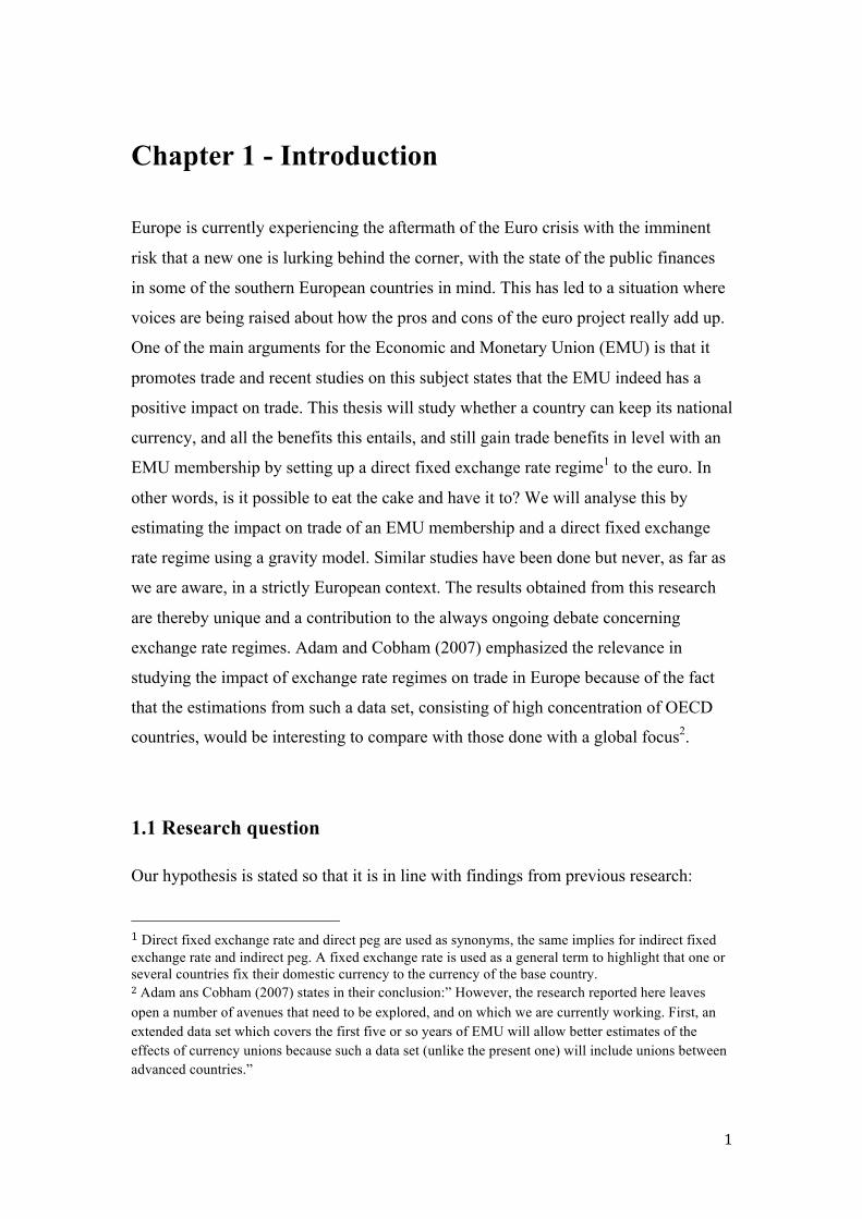
Chapter 1 - Introduction

 Europe is currently experiencing the aftermath of the Euro crisis with the imminent

risk that a new one is lurking behind the corner, with the state of the public finances

in some of the southern European countries in mind. This has led to a situation where

voices are being raised about how the pros and cons of the euro project really add up.

One of the main arguments for the Economic and Monetary Union (EMU) is that it

promotes trade and recent studies on this subject states that the EMU indeed has a

positive impact on trade. This thesis will study whether a country can keep its national

currency, and all the benefits this entails, and still gain trade benefits in level with an

EMU membership by setting up a direct fixed exchange rate regime1 to the euro. In

other words, is it possible to eat the cake and have it to? We will analyse this by

estimating the impact on trade of an EMU membership and a direct fixed exchange

rate regime using a gravity model. Similar studies have been done but never, as far as

we are aware, in a strictly European context. The results obtained from this research

are thereby unique and a contribution to the always ongoing debate concerning

exchange rate regimes. Adam and Cobham (2007) emphasized the relevance in

studying the impact of exchange rate regimes on trade in Europe because of the fact

that the estimations from such a data set, consisting of high concentration of OECD

countries, would be interesting to compare with those done with a global focus2.

1.1 Research question

Our hypothesis is stated so that it is in line with findings from previous research:

                                                                                                                         1  Direct fixed exchange rate and direct peg are used as synonyms, the same implies for indirect fixed exchange rate and indirect peg. A fixed exchange rate is used as a general term to highlight that one or several countries fix their domestic currency to the currency of the base country.  2  Adam ans Cobham (2007) states in their conclusion:” However, the research reported here leaves open a number of avenues that need to be explored, and on which we are currently working. First, an extended data set which covers the first five or so years of EMU will allow better estimates of the effects of currency unions because such a data set (unlike the present one) will include unions between advanced countries.”

 

2    

H0: During the period 2003-2012 an EMU membership has exceeded a direct fixed

exchange rate regime to the euro in terms of gains in intra-EU bilateral trade.

H1: H0 not true.

1.2 Background - The EMU and the ERM II

In 1999 the monetary system in Europe was fundamentally changed due to the

introduction of the euro. This was another step to further strengthen the market

integration in Europe that, among other things, facilitate for trade between the

European countries. The currency union initially consisted of eleven member

countries; a figure that today has been expanded to eighteen (The European

Commission, 2014). The decision to implement the euro was taken in 1992 from the

agreement of the Maastricht Treaty, which set up the rules of the introduction. Among

other things it states the conditions a country needs to meet to be able to join the

currency union. These conditions are known as the convergence criteria and address

issues as required levels of inflation, public debt, interests rates and exchange rate

fluctuations (Krugman and Obsfeldt, 2006).

One criteria concern participation in the European Monetary System’s exchange

rate mechanism (ERM II) and is of specific interest in our research since it has had

significant repercussions on the exchange rate regime landscape in Europe. The

criteria states that the member state must have participated in the ERM II for the

preceding two years without severe exchange rate fluctuations and must also not have

devalued its currency in that period. The ERM II was set up in 1999, when it replaced

the ERM, to safeguard that exchange rate fluctuations does not interfere with the

economic stability in Europe (European Commission, 2014). The operating

procedures are determined in agreement between the European Central Bank (ECB)

and the central bank of the nation in question. Fluctuation margins of +/- 15 % are set

up around an agreed central rate. The ECB has the power to initiate a procedure with

the purpose to change the rate (De Grauwe, 2012).

3    

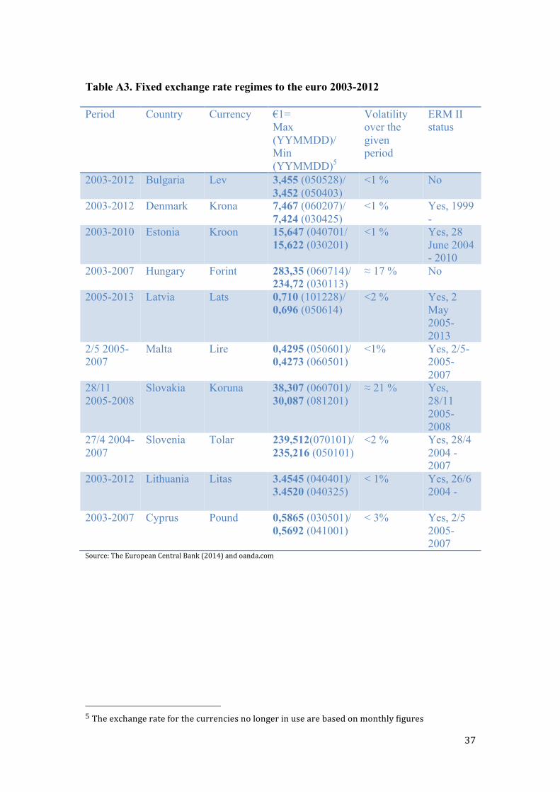
Table A3 in the appendix shows the distinct relationship between the presence of

ERM II and the amount of nations that have used a fixed exchange rate regime in

Europe during the period 2003-2012. It should be pointed out that the fluctuation

possibilities incorporated in the ERM II agreements makes it somewhat of a stretch to

call it per definition a fixed exchange rate regime. We have addressed this fact by

using exchange rate volatility terms to get a suitable selection, but more on that later.

However, the ERM II does not give the whole picture regarding the fixed exchange

rate regimes in Europe since there are countries, Bulgaria and Hungary, that have

exercised a fixed exchange rate regime in the period 2003-2012 despite not at any

time been participating in the ERM II. Both countries had problems with high levels

of inflation during the end of the 1990’s and this was a significant factor for them to

adopt a fixed exchange rate regime (Moghadam, 1998) (Gulde, 1999). Currently the

ERM II consists of only two countries, Denmark and Lithuania. Denmark has not a

pronounced intention to join the EMU but is involved in the ERM II at a +/- 2.25 %

fluctuations margin. Lithuania on the other hand has been required to postpone their

entry to the EMU because of too high levels of inflation (European Commission,

2006).

4    

Chapter 2 - Theory and previous research

2.1 Previous research

The starting point of the last decade’s research concerning common currency and

trade can be attributed to Andrew Rose (2000). Rose’s extraordinary finding that

countries using the same currency trade three times as much as they would if they

used different currencies got a major impact in the academic world. Rose studied

bilateral trade between 186 countries in the period 1970 to 1990 using a gravity model

and cross-sectional data. Since currency unions are rare, a majority of the

observations referred to trade between countries with different currencies and only

about one per cent of the observations concerned country pairs involving countries

using the same currency. Despite this fact his findings were statistically significant.

The subsequent research used Rose’s results as a benchmark and it did not take

long until criticism arose. The name of the report “Honey, I shrunk the currency union

effect on trade” quite obviously stated the author, Volker Nitsch’s, view on the topic.

Nitsch presented results that showed how minor changes in the data set, used by Rose,

got major implications in the results and he argued that the effect was exaggerated.

One substantial characteristic in the data set is that countries using a common

currency typically are small and poor, for example countries using the East Caribbean

dollar. Another characteristic in Rose’s data is small and poor countries that have

adopted a currency from a larger economy, for example island states in the Pacific

adopting the Australian dollar, a phenomenon called dollarization (Nitsch 2001).

Torsten Persson criticised the gravity model used by Rose on the basis that the

observations of trade amongst countries with the same currency were so few. Persson

stated that “Rose’s finding of a huge treatment effect of a common currency on

bilateral trade are likely to reflect systematic selection into common currencies of

country pairs with peculiar results” (Persson 2001).

If we put it in a European context; what is the EMU’s impact on bilateral trade?

Once again Andrew Rose plays a significant role with his research done together with

Eric van Wincoop (2001). Their research is an extension of Rose’s previous one and it

5    

is based on trade statistics in the period 1970 to 1995, but the authors are now making

regional breakdowns. They estimated that the eleven initial members of the EMU

would have increased their overall trade with 59 % if they had used a common

currency during the years 1970 to 1995. The statistics include multilateral residence

effects to be more accurate.

Other studies on the subject have been conducted by Faraquee (2004), Micco,

Stien and Ordonez (2003) and De Nardis and Vicarelli (2003). These all indicate that

the EMU have had a positive impact on trade, though in lesser terms then those

presented by Rose and Wincoop (2001). All studies use a similar technique, the

gravity model, but their data is comprised of slightly different variables. In summary

their estimated results indicate that the EMU has had a positive impact on bilateral

trade in the range of 2-8 % for its members.

Since the breakdown of the Bretton Woods system in the early 70’s, numerous

studies have been published to examine the impact of exchange rate volatility on trade.

The underlying concept is that less exchange rate volatility gives more stability and

should promote trade, therefore should a fixed exchange rate regime have a positive

impact on trade. Despite the logic in this there has been no coherency in the empirical

studies stating that this is true. Most studies have found no evidence that exchange

rate volatility impact trade, for example van Wincoop and Banchetta (2000) and

Tenreyro (2007). McKenzie (2002) made a compilation of previous research on this

topic and reached the conclusion that; ”the empirical literature contains the same

mixed results as the evidence provided by world trade data most commonly fails to

reveal a significant relationship. However, where a statistically significant

relationship has been derived, they indicate a positive and negative relationship

seemingly at random.”

One study with a different approach is Klein and Shambaugh’s (2004). Their

research indicates that a direct fixed exchange rate regime has a significant positive

impact on bilateral trade. Their panel data consist of 181 countries and the

observation period is 1973-1999. The result, using country pair fixed effects, implies

a 21 % increase in trade of using a direct fixed exchange rate regime compared to not

using one, everything else equal. The difference with this study, compared to previous

ones, is that the authors measure the significance on dummy variables representing if

6    

there is a direct fixed or indirect fixed exchange rate between countries. Previous

studies have estimated the effects of a fixed exchange rate on trade by multiplying the

estimated coefficients of the exchange rate volatility terms by a given change in

exchange rate volatility and exchange rate volatility squared respectively, with results

that implies minor effects of fixed exchange rates on trade. Klein and Shambaugh also

measure the effect on trade of being a member of a currency union. Their results,

using country pair fixed effects, implies that a pair of countries that are members of

the same currency union trade 38% more than an otherwise similar pair, this result is

not statistically significant though.

Adam and Cobham (2007), the research we referred to in the introduction, used

the same dummy variable estimation technique as Klein and Shambaugh (2004) but

expanded the area of interest to not only include fixed exchange rate regimes but

various ones. Using a pooled OLS gravity model they presented results indicating not

only a great treatment effect of being member of a currency union but also that a fixed

exchange rate regime fosters trade and, not the least, that it is a sliding scale,

indicating that the stronger the ties are to the base currency the greater is the positive

impact on trade. Trade between members of a currency union was 139.8 % higher

then it would be if they were non-members. Furthermore they found that if one

country was a member of a currency union and the other country pegged to this

currency, the trade increased with 56.8% compared to if this relationship did not exist.

Their results concerning if both countries have a floating regime implied a negative

impact of 17.6 % on trade. The relationships indicated by Klein and Shambaugh

(2004) and Adam and Cobham (2007) are the ones we want to study in a European

perspective since, as stated earlier, the composition of countries being members of

currency unions globally does not reflect the European context.

2.2 Theoretical framework

Even if the number of empirical studies comparing trade effects of currency unions

and fixed exchange rate regimes are limited, there are consensus among these that

currency unions foster trade to a greater extent. In this section we try to identify what

in the structure of the two regimes that cause this order. The focus is directed at the

issues of transaction costs and exchange rate uncertainty and how these affect

7    

bilateral trade.

Robert Copeland (2008) defines a monetary union as: “one (zone)3 where the

accepted means of payment consists either of a single, homogeneous currency or of

two or more currencies linked by an exchange rate that is fixed (at one for one)

irrevocably”. This definition underlines the fact that a currency union in many ways

resembles a system of fixed exchange rate regimes, but in the same time the two

systems differ in essential areas.

Robert Mundell’s theory of Optimum Currency Areas highlights two major

benefits of a common currency; the elimination of transaction costs and a better

performance of money as a medium of exchange and as a unit of account (Ricci,

2008). The Commission of the European Community (1990) describes the direct

benefits from a monetary union to be; “the elimination of exchange rate related

transaction costs and the suppression of exchange rate uncertainty”.

The matter of transaction cost is straightforward. When adopting a common

currency the need for currency exchange transactions within the currency union, and

the cost associated with these, vanish. With regards to the extreme amount of euros

traded daily in the money market, this adds up to a significant amount. Estimations

concerning the total transaction cost figure, associated with euro transactions, have

been found to be in the range of 0.25 % to 0.5 % of EU’s GDP (De Grauwe, 2012). In

this perspective the national currency is a barrier of trade since it carries transaction

costs.

The issue of exchange rate uncertainty between countries disappears if they both

adopt a common currency. The same applies if one country pegs its currency to the

other, but in this case it is a matter of the construction of the peg. The benefit of the

reduction of exchange rate uncertainty is related to the theory of the risk-averse

investor. Faced with investment or trade opportunities, investors are likely to be less

enthusiastic when the decision involves the risk of currency fluctuations (Copeland,

2008). However, the existence of forward and futures markets reduce the influence of

exchange rate fluctuations on trade and, as stated earlier, research have not been

successful in finding a causal relationship between exchange rate fluctuations and

                                                                                                                         3  Authors  remark  

8    

trade reduction. Even so, sharing a common currency is a much more serious and a

more durable commitment than a fixed exchange rate (Rose, 2000).

So far we have presented information that emphasizes benefits of a common

currency over a fixed exchange rate regime. A quick look at the European economic

landscape makes it quite clear that also this coin has two sides. The primary

disadvantage with joining a monetary union is that the country gives up its monetary

independence, which is a fundamental tool to react to changes in the economic

environment as well as strengthen the nation’s competitiveness in terms of trade

(Fregert and Jonung, 2010).

The same argument can be used against a fixed exchange rate regime. Under a

fixed exchange rate regime it is the obligation of the central bank to make sure that

the exchange rate is kept. As a consequence of this the central bank cannot deviate

from this duty by changing the money supply or interest rate if it is not in the purpose

of retaining the exchange rate (Burda and Wyplosz, 2009). The monetary

independence is therefore undermined. But what is a major difference between being

a member of a currency union and having a fixed exchange rate regime is the relative

flexibility of changing system if the current one does not benefit the country’s

economic performance. If we put this in context; it would be a much larger operation

for example Greece to leave the EMU, which has been discussed in recent years, then

it would be for Denmark to leave the ERM II. What we want to point out is that

joining a currency union is to a large extent a point of no return, a description that

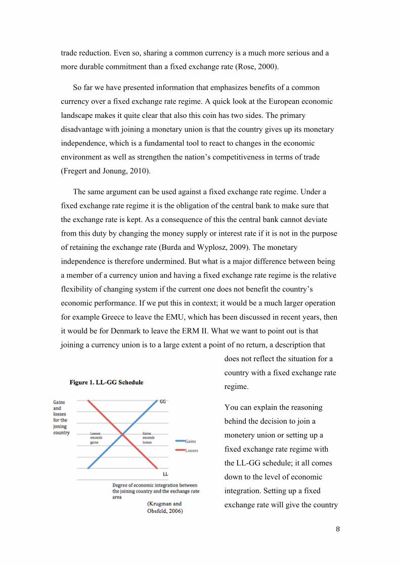
does not reflect the situation for a

country with a fixed exchange rate

regime.

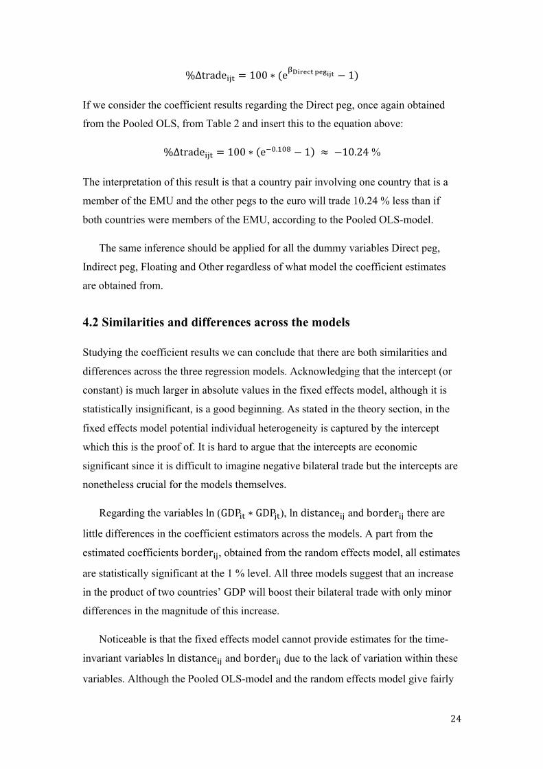
You can explain the reasoning

behind the decision to join a

monetery union or setting up a

fixed exchange rate regime with

the LL-GG schedule; it all comes

down to the level of economic

integration. Setting up a fixed

exchange rate will give the country

9    

gains in monetary efficiency, because of the removal of exchange rate fluctuations

with the currency it pegs to. Joining a currency union is one step further in the pursue

of monetary efficiency. On the other hand the country gives up its possibility of using

the exchange rate and monetary policy when either setting up a fixed exchange

regime and even more so when joining monetary union. Figure 1 shows how the level

of economic integration and the gains and losses covary. The stronger the economic

integration is the greater the incentive is in pegging the currency, or even joining the

monetary union.

 

   

 

 

 

10    

Chapter 3 - Data and Methodology

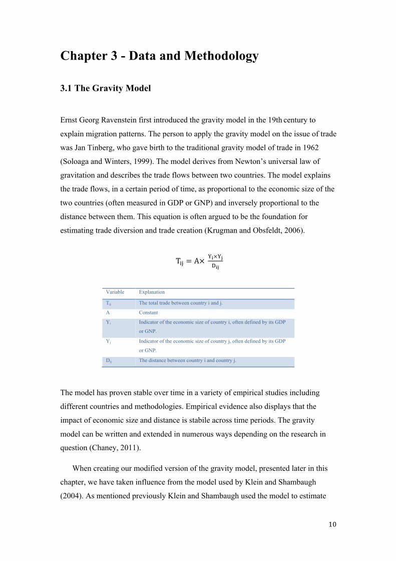
3.1 The Gravity Model

Ernst Georg Ravenstein first introduced the gravity model in the 19th century to

explain migration patterns. The person to apply the gravity model on the issue of trade

was Jan Tinberg, who gave birth to the traditional gravity model of trade in 1962

(Soloaga and Winters, 1999). The model derives from Newton’s universal law of

gravitation and describes the trade flows between two countries. The model explains

the trade flows, in a certain period of time, as proportional to the economic size of the

two countries (often measured in GDP or GNP) and inversely proportional to the

distance between them. This equation is often argued to be the foundation for

estimating trade diversion and trade creation (Krugman and Obsfeldt, 2006).

T!" = A×  !!×!!!!"

Variable Explanation

Tij The total trade between country i and j.

A Constant

Yi Indicator of the economic size of country i, often defined by its GDP

or GNP.

Yj Indicator of the economic size of country j, often defined by its GDP

or GNP.

Dij The distance between country i and country j.

The model has proven stable over time in a variety of empirical studies including

different countries and methodologies. Empirical evidence also displays that the

impact of economic size and distance is stabile across time periods. The gravity

model can be written and extended in numerous ways depending on the research in

question (Chaney, 2011).

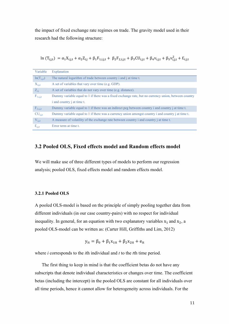
When creating our modified version of the gravity model, presented later in this

chapter, we have taken influence from the model used by Klein and Shambaugh

(2004). As mentioned previously Klein and Shambaugh used the model to estimate

11    

the impact of fixed exchange rate regimes on trade. The gravity model used in their

research had the following structure:

ln  (T!,!,!)  = α!X!,!,! + α!Z!,! + β!F!,!,!,! +  β!F!,!,!,! + β!CU!,!,! + β!v!,!,! + β!v!,!,!! + Ɛ!,!,! Variable Explanation ln(Ti,j,t) The natural logarithm of trade between country i and j at time t. Xi,j,t A set of variables that vary over time (e.g. GDP). Zi,j A set of variables that do not vary over time (e.g. distance). F1,i,j,t Dummy variable equal to 1 if there was a fixed exchange rate, but no currency union, between country

i and country j at time t. F2,i,j,t Dummy variable equal to 1 if there was an indirect peg between country i and country j at time t. CUi,j,t Dummy variable equal to 1 if there was a currency union amongst country i and country j at time t. Vi,j,t A measure of volatility of the exchange rate between country i and country j at time t. Ɛi,j,t Error term at time t.

3.2 Pooled OLS, Fixed effects model and Random effects model

We will make use of three different types of models to perform our regression

analysis; pooled OLS, fixed effects model and random effects model.

3.2.1 Pooled OLS

A pooled OLS-model is based on the principle of simply pooling together data from

different individuals (in our case country-pairs) with no respect for individual

inequality. In general, for an equation with two explanatory variables x! and x!, a

pooled OLS-model can be written as: (Carter Hill, Griffiths and Lim, 2012)

y!" = β! + β!x!"# + β!x!"# + e!"

where i corresponds to the ith individual and t to the tth time period.

The first thing to keep in mind is that the coefficient betas do not have any

subscripts that denote individual characteristics or changes over time. The coefficient

betas (including the intercept) in the pooled OLS are constant for all individuals over

all time periods, hence it cannot allow for heterogeneity across individuals. For the

12    

OLS estimators to be unbiased and consistent this exogeneity assumption must be

fulfilled.

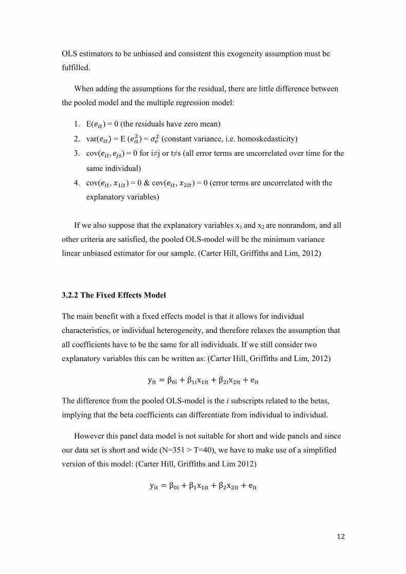
When adding the assumptions for the residual, there are little difference between

the pooled model and the multiple regression model:

1. E(𝑒!") = 0 (the residuals have zero mean)

2. var(𝑒!") = E (𝑒!"! ) = 𝜎!! (constant variance, i.e. homoskedasticity)

3. cov(𝑒!" , 𝑒!") = 0 for i≠j or t≠s (all error terms are uncorrelated over time for the

same individual)

4. cov(𝑒!",  𝑥!!") = 0 & cov(𝑒!",  𝑥!!") = 0 (error terms are uncorrelated with the

explanatory variables)

If we also suppose that the explanatory variables x1 and x2 are nonrandom, and all

other criteria are satisfied, the pooled OLS-model will be the minimum variance

linear unbiased estimator for our sample. (Carter Hill, Griffiths and Lim, 2012)

3.2.2 The Fixed Effects Model

The main benefit with a fixed effects model is that it allows for individual

characteristics, or individual heterogeneity, and therefore relaxes the assumption that

all coefficients have to be the same for all individuals. If we still consider two

explanatory variables this can be written as: (Carter Hill, Griffiths and Lim, 2012)

y!" = β!" + β!"x!"# + β!"x!"# + e!"

The difference from the pooled OLS-model is the i subscripts related to the betas,

implying that the beta coefficients can differentiate from individual to individual.

However this panel data model is not suitable for short and wide panels and since

our data set is short and wide (N=351 > T=40), we have to make use of a simplified

version of this model: (Carter Hill, Griffiths and Lim 2012)

y!" = β!" + β!x!"# + β!x!"# + e!"

13    

The i subscripts for the parameter betas (𝛽!  𝑎𝑛𝑑  𝛽!) are gone which implies that these

parameters are treated as constants for all individuals. The differences in behavioral

characteristics between individuals, or heterogeneity, are now assumed to be captured

by the intercept (𝛽!!). This is the key feature of a fixed effects model that the

individual intercepts (often called fixed effects) are included to control for

characteristics that are distinctive for one individual and that does not change over

time.

The estimation technique we will make use of is called the fixed effects estimator

and since our number of individuals (country-pairs) is relatively large this will be the

most appropriate technique to use. We will illustrate this estimation technique below

with the simplified fixed effects model as our starting point: (Carter Hill, Griffiths and

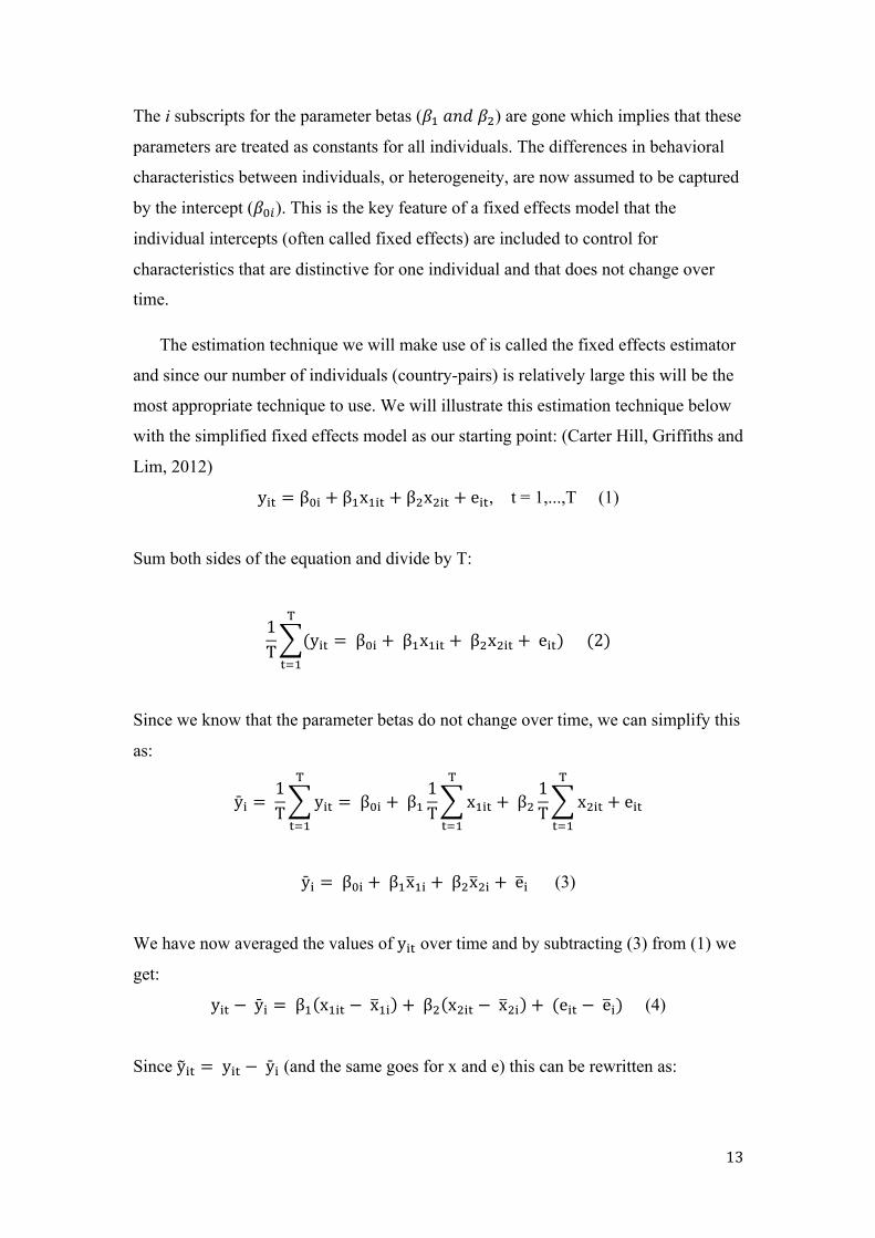
Lim, 2012)

y!" = β!" + β!x!"# + β!x!"# + e!", t = 1,...,T (1)

Sum both sides of the equation and divide by T:

1T (y!" =  β!" +  β!x!"# +  β!x!"# +  e!")

!

!!!

         (2)

Since we know that the parameter betas do not change over time, we can simplify this

as:

ӯ! =  1T y!"

!

!!!

=  β!" +  β!1T x!"#

!

!!!

+  β!1T x!"#

!

!!!

+ e!"

ӯ! =  β!" +  β!x!" +  β!x!" +  e! (3)

We have now averaged the values of y!" over time and by subtracting (3) from (1) we

get:  

y!" −  ӯ! =  β! x!"# −  x!" +  β! x!"# −  x!" +  (e!" −  e!) (4)

Since y!" =  y!" −  ӯ! (and the same goes for x and e) this can be rewritten as:

14    

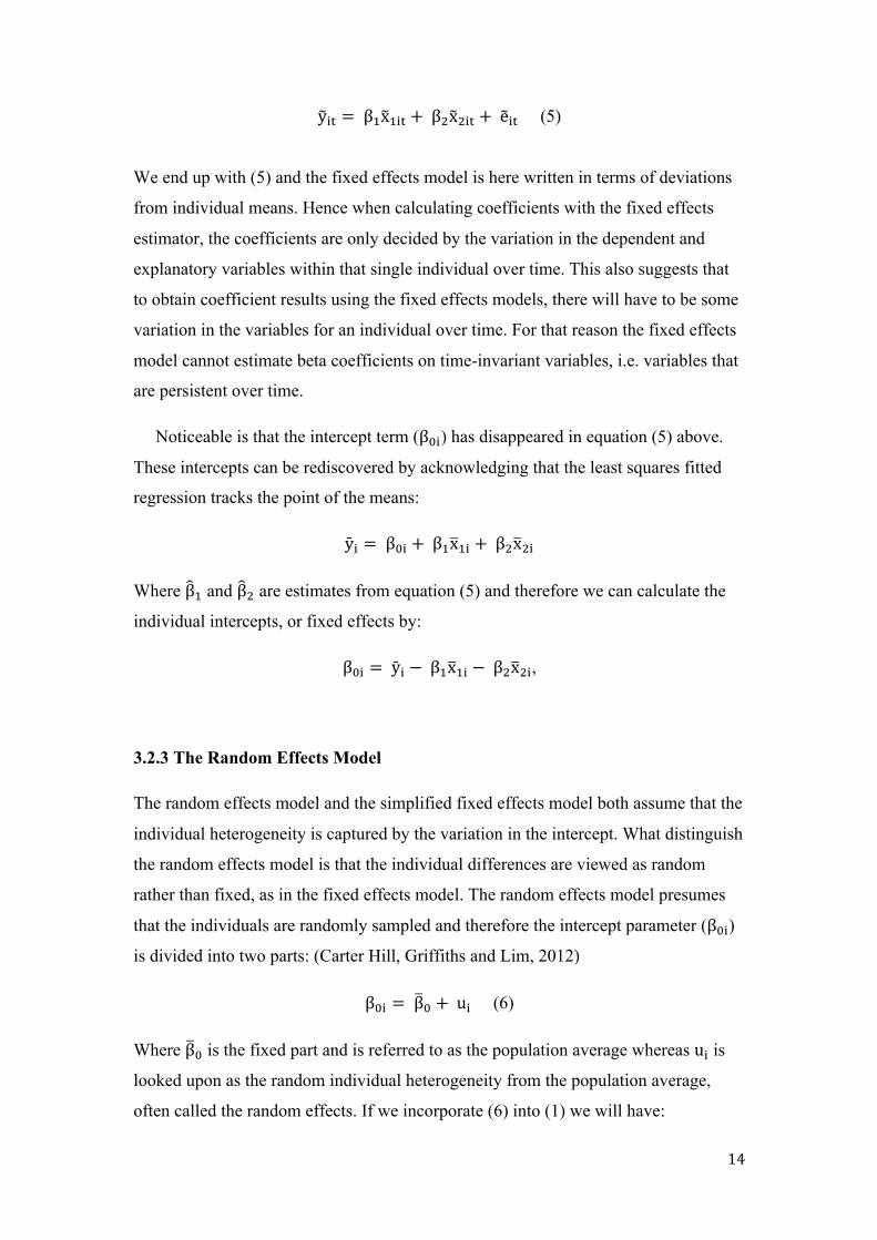
y!" =  β!x!"# +  β!x!"# +  e!" (5)

We end up with (5) and the fixed effects model is here written in terms of deviations

from individual means. Hence when calculating coefficients with the fixed effects

estimator, the coefficients are only decided by the variation in the dependent and

explanatory variables within that single individual over time. This also suggests that

to obtain coefficient results using the fixed effects models, there will have to be some

variation in the variables for an individual over time. For that reason the fixed effects

model cannot estimate beta coefficients on time-invariant variables, i.e. variables that

are persistent over time.

Noticeable is that the intercept term (β!") has disappeared in equation (5) above.

These intercepts can be rediscovered by acknowledging that the least squares fitted

regression tracks the point of the means:

ӯ! =  β!" +  β!x!" +  β!x!"

Where β! and β! are estimates from equation (5) and therefore we can calculate the

individual intercepts, or fixed effects by:

β!" =  ӯ! −  β!x!" −  β!x!",

3.2.3 The Random Effects Model

The random effects model and the simplified fixed effects model both assume that the

individual heterogeneity is captured by the variation in the intercept. What distinguish

the random effects model is that the individual differences are viewed as random

rather than fixed, as in the fixed effects model. The random effects model presumes

that the individuals are randomly sampled and therefore the intercept parameter (β!")

is divided into two parts: (Carter Hill, Griffiths and Lim, 2012)

β!" =  β! +  u! (6)

Where β! is the fixed part and is referred to as the population average whereas u! is

looked upon as the random individual heterogeneity from the population average,

often called the random effects. If we incorporate (6) into (1) we will have:

15    

y!" = (β! +  u!)+ β!x!"# + β!x!"# + e!" (7)

Rearranging terms will make us end up with:

y!" = β! + β!x!!" + β!x!"# + (e!" +  u!)

y!" = β! + β!x!"# + β!x!"# +  v!" (8)

The β! is now the intercept parameter and the error term v!" carries both the usual

error term that we looked at earlier (e!") and the random individual effect (u!). The

combined error term in a random effects model can be given by:

v!" =  u! +  e!"

The major difference regarding the residual assumptions in the random effects model

and the pooled OLS-model is that the errors terms for the same individual are

assumed to be correlated over time: (Carter Hill, Griffiths and Lim, 2012)

1. E(v!") = 0 (the residuals have zero mean)

2. var(v!") =  σ!! +  σ!! (constant variance, i.e. homoskedasticity)

3. cov(v!", v!") = σ!! for t≠s (error terms for individual i are correlated)

4. cov(v!", v!") = 0 for i≠j (error terms for different individuals are uncorrelated)

5. cov (e!",  x!"#) = 0 & cov (e!",  x!"#) = 0 (error term e!" are uncorrelated with the

explanatory variables)

6. cov (u!",  x!"#) = 0 & cov (u!",  x!"#) = 0 (random effects are uncorrelated with

the explanatory variables)

3.2.4 The Breusch-Pagan Lagrange Multiplier (LM)

When coefficient results have been obtained from the Pooled OLS-model, the fixed

effects model and the random effects model we will perform a Breusch-Pagan (LM)

test to determine whether the Pooled OLS-model is an appropriate estimation

technique that fits the purpose of this thesis report.

The Breusch-Pagan test will help to examine if there is individual heterogeneity to

account for across our data sample. The random individual effect (u!) and the

assumptions for the residuals in the random effects model, both discussed above, are

16    

the key components for this test alongside with the correlation equation given by:

(Carter Hill, Griffiths and Lim, 2012)

ρ = corr   v!", v!" =cov  (v!", v!")var v!" var(v!")

=  σ!!

σ!! + σ!!              t ≠ s

Suppose if σ!! = 0 this will lead to ρ = 0 and we can therefore conclude that

differences amongst the individuals in our data set occur. The Breusch-Pagan test is

consequently a simple hypothesis test stated by:

H!:  σ!! = 0

H!:  σ!! ≠ 0

If the null hypothesis can be rejected when performing the Breusch-Pagan test we can

be assured that random individual effects are present in the data sample and the

pooled OLS-model will be biased and inconsistent estimating the coefficient results.

If this is the case, then the pooled OLS-model is disqualified as an estimation

technique and we have to put our faith to either the fixed effects model or the random

effects model.

3.2.5 Hausman test

To decide whether to apply the fixed effects model or the random effects model, in

case the null hypothesis is rejected in the Breusch-Pagan test, a Hausman test is

appropriate for making this decision.

The basic theory behind the Hausman test is that if there is no correlation between

the random individual effect (u!) and any of the explanatory variables, then both the

fixed effects model and the random effects will be consistent and generate estimators

that in large samples will merge into the true beta parameters. However, if there is

correlation between (u!) and any of the explanatory variables, the random effects

model will be inconsistent and in large samples not converge into the true beta

parameters, whilst the fixed effects model still would generate consistent parameters.

In the presence of the correlation mentioned previously, we can expect differences in

the estimates obtained from the two models. (Carter Hill, Griffiths and Lim, 2012)

17    

The hypothesis testing connected to the Hausman test is as follows:

H!:Corr  u!, x!"# =  0

H!:Corr  u!, x!"# ≠  0

Hence if the null hypothesis is rejected when performing the Hausman test, the

random effect models estimation parameters will be misleading and the fixed effects

model should be put to practice.

A vital shortcoming of the Hausman test is that it cannot be exercised in

combination with cluster-robust standard errors. The method of cluster-robust

standard errors liberates the assumptions regarding the standard errors and this causes

violations in the assumptions for the Hausman test.

3.3 Our Regression Model

As mentioned previously our regression model is influenced by the regression model

used by Klein and Shambaugh (2004). The two models differentiate regarding the

classification scheme of exchange rate regimes that are not classified as a currency

union, direct peg or indirect peg. We will not include exchange rate volatility as one

of the explanatory variables. This is because of the problem, discussed in section 2.1,

to find a causal relationship between exchange rate volatility and bilateral trade - even

when you do so the economic significance can be either positive or negative. Also, we

are not studying the effects of exchange rate volatility on bilateral trade in the EU but

the exchange rate regimes as such, hence the exclusion of this term from our model.

ln  (  T!,!,!) =  β!ln(GDP!" ∗ GDP!")+ β!ln  (Distance!")+ β!Border!,! + β!CU!,!,!+  β!Direct  peg!,!,! +  β!Indirect  peg  !,!,! + β!Floating!,!,!+ β!Other!,!,! + β!quarter! +  ε!,!,!

where: i = 1,2,… ,N

j = 1,2,… ,N i ≠ j

t = 1, 2,… ,T

18    

Variable Explanation 𝐥𝐧  (  𝐓𝐢,𝐣,𝐭) Dependent variable. The natural logarithm of trade between

country i and country j at time t. Time-variant variable. 𝐥𝐧(𝐆𝐃𝐏𝐢𝐭 ∗ 𝐆𝐃𝐏𝐣𝐭) The natural logarithm of the product of GDP in country i and

country j at time t. Time-variant variable.

𝐥𝐧  (𝐃𝐢𝐬𝐭𝐚𝐧𝐜𝐞𝐢𝐣) The natural logarithm of distance between country i and country j in kilometres. Time-invariant variable.

𝐁𝐨𝐫𝐝𝐞𝐫𝐢,𝐣 Dummy variable equal to 1 if the counties share a land border. Time-invariant variable.

𝐂𝐔𝐢,𝐣,𝐭   Dummy variable equal to 1 if country i and country j are members of the EMU at time t. Time-variant variable.

𝐃𝐢𝐫𝐞𝐜𝐭  𝐩𝐞𝐠𝐢,𝐣,𝐭 Dummy variable equal to 1 if country i or country j is a member of the EMU and the other country has a fixed exchange rate to the euro at time t. Time-variant variable.

𝐈𝐧𝐝𝐢𝐫𝐞𝐜𝐭  𝐩𝐞𝐠𝐢,𝐣,𝐭 Dummy variable equal to 1 if country i and country j have a fixed exchange rate to the euro at time t. Time-variant variable

𝐅𝐥𝐨𝐚𝐭𝐢𝐧𝐠𝐢,𝐣,𝐭 Dummy variable equal to 1 if there is a floating exchange rate between country i and country j at time t. Time-variant variable.

𝐎𝐭𝐡𝐞𝐫𝐢,𝐣,𝐭 Dummy variable equal to 1 if country i or country j has a fixed exchange rate to a currency basket and the other country does not have a floating exchange rate at time t. Or if country i or country j has a fixed exchange rate to the Euro with a volatility exceeding 2% in a given year and the other country does not have a floating exchange rate at time t. Time-variant variable.

𝐪𝐮𝐚𝐫𝐭𝐞𝐫𝐭 Dummy variable equal to 1 for all observations in a given quarter.

𝛆𝐢,𝐣,𝐭 Error term. Time-variant variable.

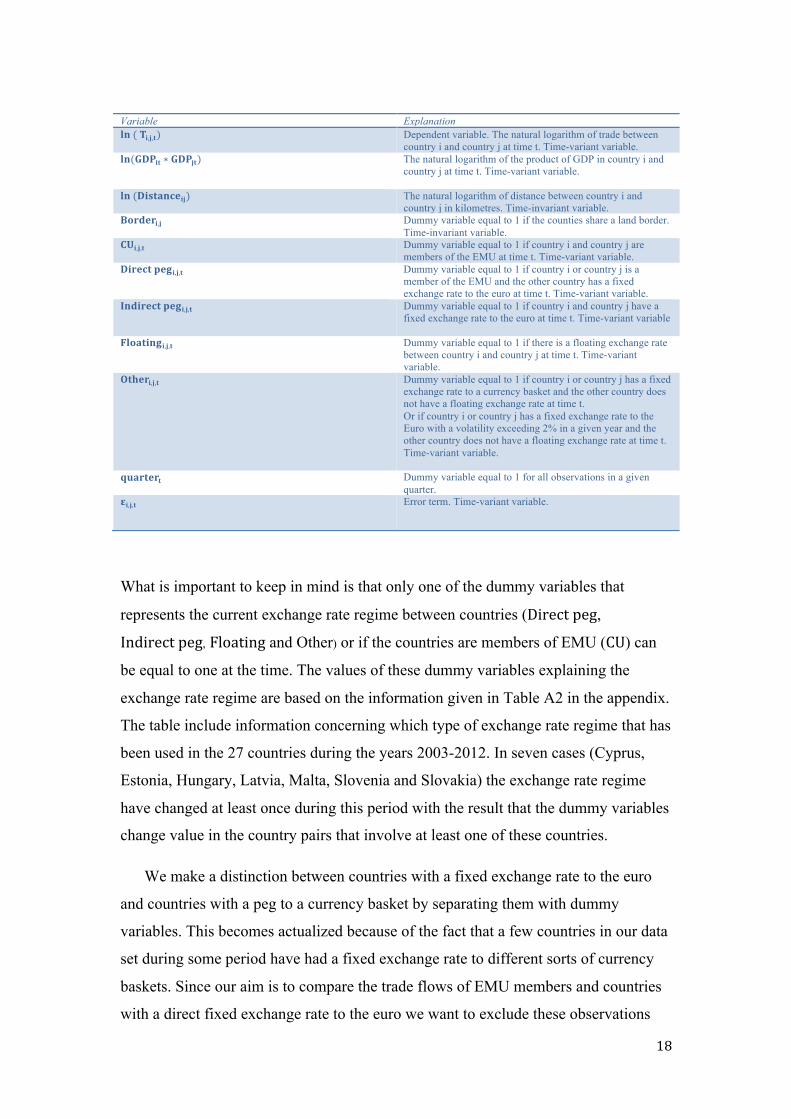
What is important to keep in mind is that only one of the dummy variables that

represents the current exchange rate regime between countries (Direct  peg,

Indirect  peg, Floating and Other) or if the countries are members of EMU (CU) can

be equal to one at the time. The values of these dummy variables explaining the

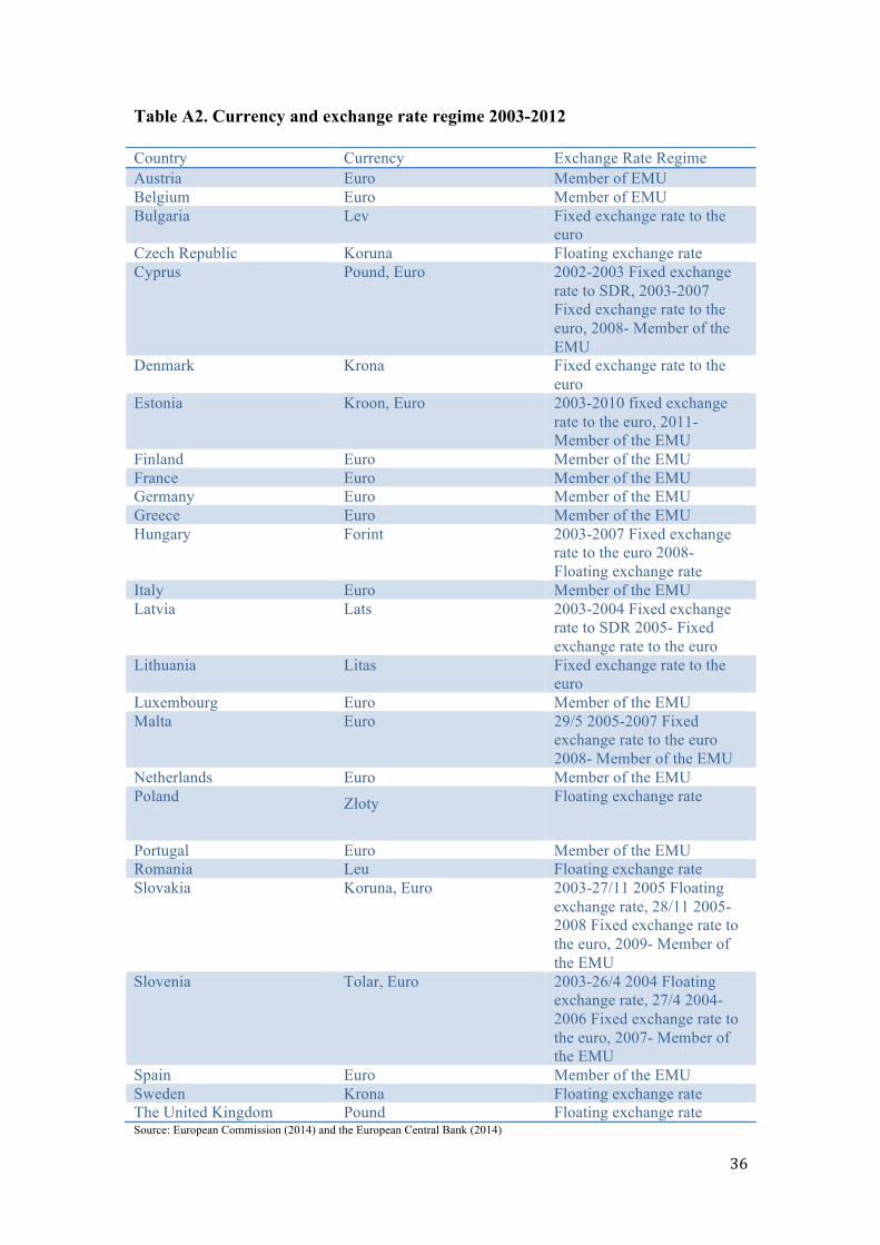
exchange rate regime are based on the information given in Table A2 in the appendix.

The table include information concerning which type of exchange rate regime that has

been used in the 27 countries during the years 2003-2012. In seven cases (Cyprus,

Estonia, Hungary, Latvia, Malta, Slovenia and Slovakia) the exchange rate regime

have changed at least once during this period with the result that the dummy variables

change value in the country pairs that involve at least one of these countries.

We make a distinction between countries with a fixed exchange rate to the euro

and countries with a peg to a currency basket by separating them with dummy

variables. This becomes actualized because of the fact that a few countries in our data

set during some period have had a fixed exchange rate to different sorts of currency

baskets. Since our aim is to compare the trade flows of EMU members and countries

with a direct fixed exchange rate to the euro we want to exclude these observations

19    

from impacting the Direct  peg dummy and therefore we have created a dummy

variable, Other, whose purpose is to collect these observations.

We also make a distinction between countries with a direct and indirect fixed

exchange rate. We illustrate the difference with an example; Denmark and Bulgaria

have had a fixed exchange rate to the euro during the entire sample period, 2003-2012,

resulting in that the Direct peg dummy is equal to 1 in the country pairs involving

Denmark or Bulgaria and any member of the EMU. As a consequence of the two

countries’ exchange rate regime there is an indirect fixed exchange rate between the

two countries in question and we devote a dummy variable, Indirect peg, for

observations of this kind.

To account for time trends and seasonality we have included forty dummy

variables, one for each quarter of observation. These are included only for controlling

purposes.

Table A3 in the appendix shows the maximum and minimum exchange rates for

the currencies that during at least some part of the period 2003-2012 have been

pegged to the euro. The volatility term clearly indicates that there have been

differences in the way the fixed exchange rate regimes have been constructed and

implemented. All countries besides Bulgaria and Hungary have been, or are, members

of the ERM II and the volatility terms indicates that they have used the fluctuation

possibility in the ERM II agreements in different fashion. We have made a

classification scheme for those countries with a peg to the euro, proceeded from the

classification used by Klein and Shambaugh (2004). Therefore a particular country

with a peg to the euro is judged to have a direct peg if the exchange rate volatility,

between the domestic currency and the euro, stays within a +/- 2 per cent band in a

given year. We do not need to make any further distinctions here since the only two

countries that have experienced exchange rate fluctuations exceeding these yearly

limitations are Hungary (in five consecutive years between 2003 and 2007) and

Slovakia (between year 2006 and 2008). The observations not eligible as direct pegs

will be placed in the Other dummy. Given that the purpose of our analysis is to

highlight the difference in trade flows among members of the EMU and countries

with a direct peg to the euro, we will not suffer from adding these observations in the

Other dummy – as the results provided from the variable Other is not of interest to us.

20    

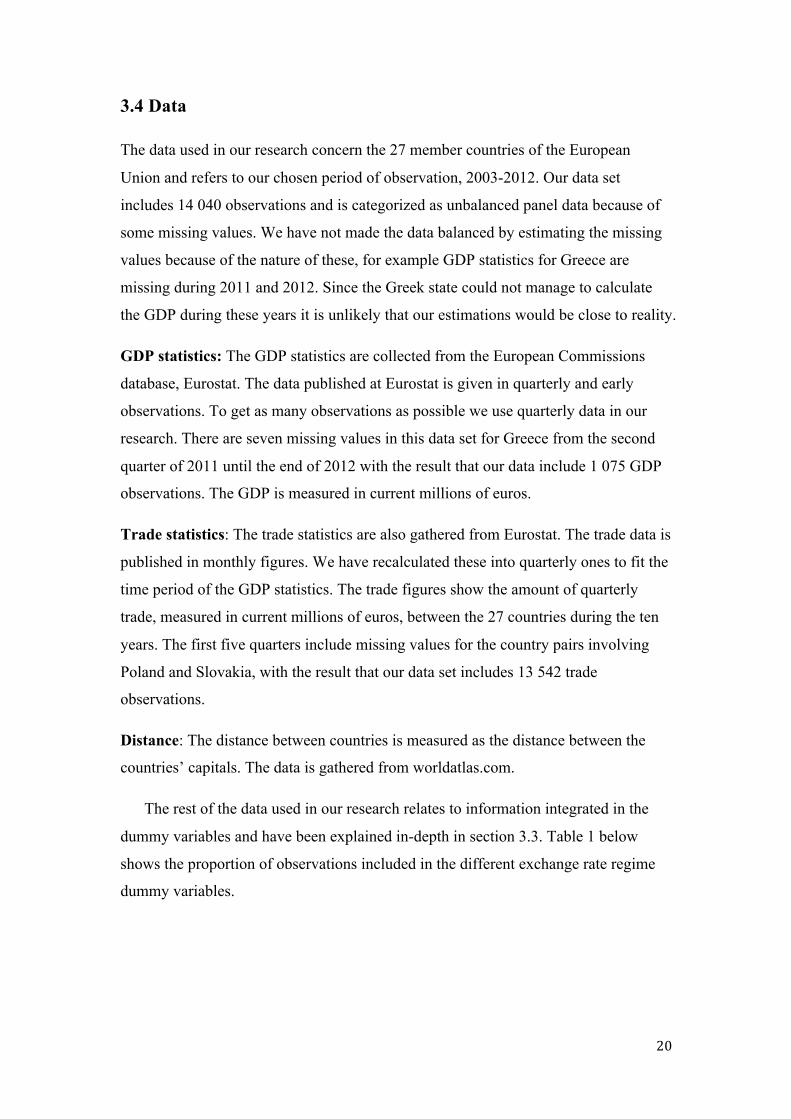
3.4 Data

The data used in our research concern the 27 member countries of the European

Union and refers to our chosen period of observation, 2003-2012. Our data set

includes 14 040 observations and is categorized as unbalanced panel data because of

some missing values. We have not made the data balanced by estimating the missing

values because of the nature of these, for example GDP statistics for Greece are

missing during 2011 and 2012. Since the Greek state could not manage to calculate

the GDP during these years it is unlikely that our estimations would be close to reality.

GDP statistics: The GDP statistics are collected from the European Commissions

database, Eurostat. The data published at Eurostat is given in quarterly and early

observations. To get as many observations as possible we use quarterly data in our

research. There are seven missing values in this data set for Greece from the second

quarter of 2011 until the end of 2012 with the result that our data include 1 075 GDP

observations. The GDP is measured in current millions of euros.

Trade statistics: The trade statistics are also gathered from Eurostat. The trade data is

published in monthly figures. We have recalculated these into quarterly ones to fit the

time period of the GDP statistics. The trade figures show the amount of quarterly

trade, measured in current millions of euros, between the 27 countries during the ten

years. The first five quarters include missing values for the country pairs involving

Poland and Slovakia, with the result that our data set includes 13 542 trade

observations.

Distance: The distance between countries is measured as the distance between the

countries’ capitals. The data is gathered from worldatlas.com.

The rest of the data used in our research relates to information integrated in the

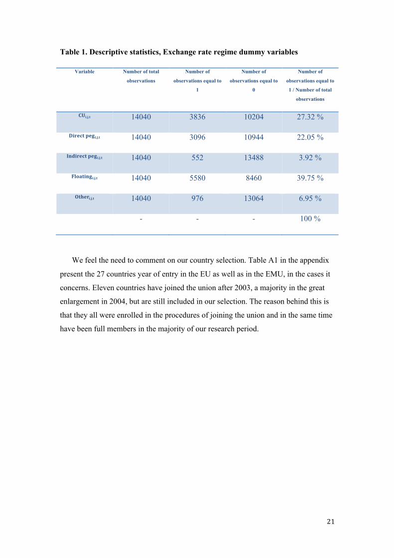
dummy variables and have been explained in-depth in section 3.3. Table 1 below

shows the proportion of observations included in the different exchange rate regime

dummy variables.

21    

Table 1. Descriptive statistics, Exchange rate regime dummy variables

Variable Number of total

observations

Number of

observations equal to

1

Number of

observations equal to

0

Number of

observations equal to

1 / Number of total

observations

𝐂𝐔𝐢,𝐣,𝐭 14040 3836 10204 27.32 %

𝐃𝐢𝐫𝐞𝐜𝐭  𝐩𝐞𝐠𝐢,𝐣,𝐭 14040 3096 10944 22.05 %

𝐈𝐧𝐝𝐢𝐫𝐞𝐜𝐭  𝐩𝐞𝐠𝐢,𝐣,𝐭 14040 552 13488 3.92 %

𝐅𝐥𝐨𝐚𝐭𝐢𝐧𝐠𝐢,𝐣,𝐭 14040 5580 8460 39.75 %

𝐎𝐭𝐡𝐞𝐫𝐢,𝐣,𝐭 14040 976 13064 6.95 %

- - - 100 %

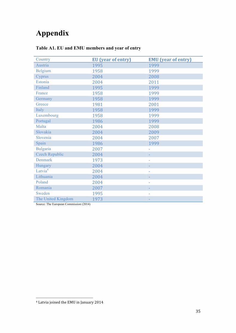
We feel the need to comment on our country selection. Table A1 in the appendix

present the 27 countries year of entry in the EU as well as in the EMU, in the cases it

concerns. Eleven countries have joined the union after 2003, a majority in the great

enlargement in 2004, but are still included in our selection. The reason behind this is

that they all were enrolled in the procedures of joining the union and in the same time

have been full members in the majority of our research period.

   

 

 

22    

Chapter 4 - Results and analysis  

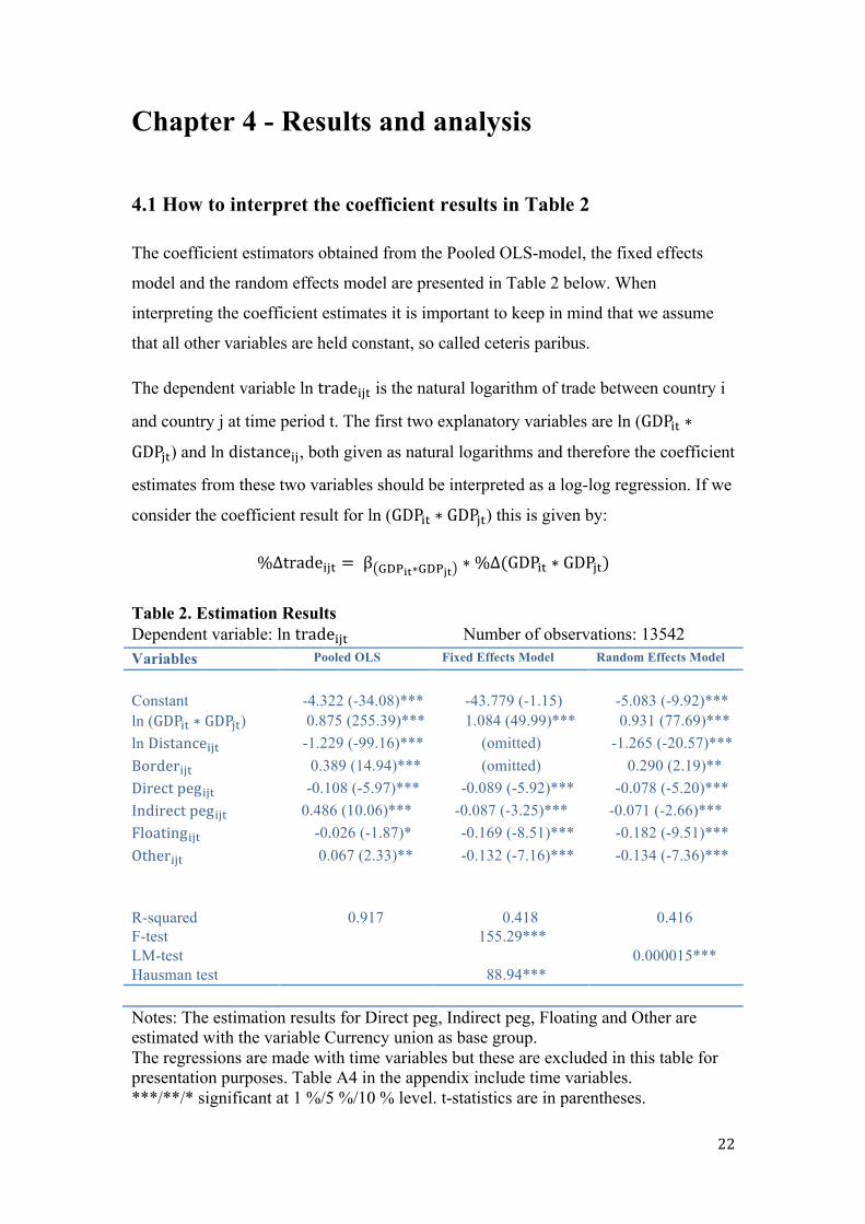
4.1 How to interpret the coefficient results in Table 2  The coefficient estimators obtained from the Pooled OLS-model, the fixed effects

model and the random effects model are presented in Table 2 below. When

interpreting the coefficient estimates it is important to keep in mind that we assume

that all other variables are held constant, so called ceteris paribus.

The dependent variable ln trade!"# is the natural logarithm of trade between country i

and country j at time period t. The first two explanatory variables are ln (GDP!" ∗

GDP!") and ln distance!", both given as natural logarithms and therefore the coefficient

estimates from these two variables should be interpreted as a log-log regression. If we

consider the coefficient result for ln (GDP!" ∗ GDP!") this is given by:

%Δtrade!"# =  β !"#!"∗!"#!" ∗%Δ(GDP!" ∗ GDP!")

Table 2. Estimation Results Dependent variable: ln trade!"# Number of observations: 13542 Variables Pooled OLS Fixed Effects Model Random Effects Model

Constant -4.322 (-34.08)*** -43.779 (-1.15) -5.083 (-9.92)*** ln (GDP!" ∗ GDP!") 0.875 (255.39)*** 1.084 (49.99)*** 0.931 (77.69)*** ln Distance!"# -1.229 (-99.16)*** (omitted) -1.265 (-20.57)*** Border!"# 0.389 (14.94)*** (omitted) 0.290 (2.19)** Direct  peg!"# -0.108 (-5.97)*** -0.089 (-5.92)*** -0.078 (-5.20)*** Indirect  peg!"# 0.486 (10.06)*** -0.087 (-3.25)*** -0.071 (-2.66)*** Floating!"# -0.026 (-1.87)* -0.169 (-8.51)*** -0.182 (-9.51)*** Other!"# 0.067 (2.33)** -0.132 (-7.16)*** -0.134 (-7.36)*** R-squared F-test LM-test Hausman test

0.917 0.418 155.29***

88.94***

0.416

0.000015***

Notes: The estimation results for Direct peg, Indirect peg, Floating and Other are estimated with the variable Currency union as base group. The regressions are made with time variables but these are excluded in this table for presentation purposes. Table A4 in the appendix include time variables. ***/**/* significant at 1 %/5 %/10 % level. t-statistics are in parentheses.

23    

Let us suppose that the product of GDP between countries i and j increase with 1 % at

time t, everything else held constant. The beta coefficient related to GDP!" ∗ GDP!" is

0.875, using the Pooled OLS-model, we thereby get:

%Δtrade!"# =  0.875 ∗ 1  % = 0.875  %

Accordingly, if (GDP!" ∗ GDP!") increase with 1 % we would expect a 0.875 %

increase in trade between the two countries i and j, ceteris paribus, given the Pooled

OLS estimators. The same interpretation should be used for all estimates regarding ln

(GDP!" ∗ GDP!") and ln distance!".

The next explanatory variable, border!", is a dummy variable given the value 1 if

the countries i and j share a border and 0 if they do not. The estimated beta

coefficients of border!" should be interpreted as the effect on bilateral trade if

countries i and j share a border. Since the dependent variable is expressed as a natural

logarithm, the exact percentage change in trade!"# given a movement in the dummy

variable from 0 to 1 is:

%Δtrade!"# = 100 ∗ (e!!"#$%#!" − 1)

Reading of the Table 2 above, the border!"  beta coefficient obtained from the Pooled

OLS-model is 0.389, inserting this figure in the equation above gives us:

%Δtrade!"# = 100 ∗ e!.!"# − 1 ≈ 47.55 %

The bilateral trade for two countries within the European Union in general is 47.55 %

higher if the country pair shares a border compared to if they do not, during the period

2003 to 2012 given the Pooled OLS estimates. All three coefficient results from the

variable border!" should be understood in the same way as described above.

What is significant to remember regarding the dummy variables Direct peg,

Indirect peg, Floating and Other is that their coefficient estimates stand in comparison

to the base group, CU. The coefficient results for Direct peg should consequently

thereby be taken as the effects on bilateral trade between countries i and j at time

period t, for applying a direct fixed exchange rate regime instead of both being

members of the EMU. The exact percentage change is given by:

24    

%Δtrade!"# = 100 ∗ (e!!"#$%&  !"#!"# − 1)

If we consider the coefficient results regarding the Direct peg, once again obtained

from the Pooled OLS, from Table 2 and insert this to the equation above:

%Δtrade!"# = 100 ∗ e!!.!"# − 1  ≈  −10.24 %

The interpretation of this result is that a country pair involving one country that is a

member of the EMU and the other pegs to the euro will trade 10.24 % less than if

both countries were members of the EMU, according to the Pooled OLS-model.

The same inference should be applied for all the dummy variables Direct peg,

Indirect peg, Floating and Other regardless of what model the coefficient estimates

are obtained from.

4.2 Similarities and differences across the models  Studying the coefficient results we can conclude that there are both similarities and

differences across the three regression models. Acknowledging that the intercept (or

constant) is much larger in absolute values in the fixed effects model, although it is

statistically insignificant, is a good beginning. As stated in the theory section, in the

fixed effects model potential individual heterogeneity is captured by the intercept

which this is the proof of. It is hard to argue that the intercepts are economic

significant since it is difficult to imagine negative bilateral trade but the intercepts are

nonetheless crucial for the models themselves.

Regarding the variables ln (GDP!" ∗ GDP!"), ln distance!" and border!" there are

little differences in the coefficient estimators across the models. A part from the

estimated coefficients  border!", obtained from the random effects model, all estimates

are statistically significant at the 1 % level. All three models suggest that an increase

in the product of two countries’ GDP will boost their bilateral trade with only minor

differences in the magnitude of this increase.

Noticeable is that the fixed effects model cannot provide estimates for the time-

invariant variables ln distance!" and border!" due to the lack of variation within these

variables. Although the Pooled OLS-model and the random effects model give fairly

25    

consistent estimations of these two variables. If the distance between country i and

country j increase by 1 % the Pooled OLS predicts a decrease in bilateral trade by

1.229 %, whilst the random effects model suggests a decrease by 1.265 %.

The effects of two countries sharing a border on bilateral trade are as follows:

Pooled  OLS ∶  %Δtrade!"# = 100 ∗ e!.!"# − 1 ≈ 47.55 %

Random  effects  model ∶ %Δtrade!"# = 100 ∗ e!.!"# − 1 ≈ 33.64  %

The bilateral trade for two countries within the European Union is in general 47.55 %

higher if the country pair shares a border compared to if they do not, during the period

2003 to 2012 given the Pooled OLS estimates. The corresponding figure using the

random effects model is 33.64 %.

The major distinctions in the results are found when we evaluate the coefficient

estimations for the dummy variables Direct peg, Indirect peg, Floating and Other. The

fixed effects model and the random effects model give consistent rankings and the

magnitude of the coefficient results do not differ sufficiently. However, the results

from the Pooled OLS-model provide us with a completely different set of rankings.

According to the results from the Pooled OLS if a country pair’s exchange rate

regime is characterized as Indirect peg or Other, the two countries would be better off

than if both countries were a part of the EMU – in terms of bilateral trade. An indirect

peg would increase trade between country i and country j by 62.58 % compared to if

both countries i and j were members of the EMU, according to the Pooled OLS

estimation. Whilst the fixed effects model suggests a decrease in bilateral trade by

8.33 % and the random effects model a decrease by 6.85 %.

Another difference is that the R-square is much higher with the Pooled OLS-

model compared to the two others. The difference occurs due to the fact that in the

fixed effects model and the random effects model the intercept captures the individual

heterogeneity or random effects. Due to shortcomings in the estimation technique, the

explanatory powers in the intercept are lost in the fixed effects model and the random

effects model. Therefore, in reality, there are no differences in explanatory power

across the three models.

26    

4.3 Breusch-Pagan test  To conclude whether the coefficient results obtained from the Pooled OLS-model, the

fixed effects model or the random effects model reflects the true parameter betas to

the greatest extent – we have performed a Breusch-Pagan test (LM-test). This test will

help us to assess if the results from the Pooled OLS-model are reliable and consistent

given the nature of our dataset. If not, we have to apply the fixed effects model or the

random effects model to justify the results from our regression model.

The LM test basically examines if there are random individual effects across

entities. The null hypothesis can thereby be simplified and interpreted as that there are

no individual heterogeneity present across country pairs.

The outcome of the Breusch-Pagan test is both unambiguous and persuasive,

displayed in Table A5 in the appendix, as it rejects the null hypothesis at any of the

conventional significance levels. Hence we can rule out the theory that there are no

individual differences amongst the country pairs in our sample, or in other words that

the bilateral trade is determined by identical factors within all country pairs.

The presence of individual differences between the country pairs in our sample is,

in hindsight, rational since we are dealing with such a complex greatness as bilateral

trade between countries. The driving forces of trade between one country pair are not

equal to the driving forces of trade for another country pair. The differences can be

attributed to country-specific conditions that arise due to inequality in for example

social, economical, political, geographical and historical matters.

The Pooled OLS-model cannot allow for heterogeneity for its estimators to be

unbiased and consistent. Through the Breusch-Pagan test we have proved that

individual heterogeneity is present in our data set and therefore we can disqualify the

Pooled OLS-model as the best suitable estimation technique for our regression

analysis. Hence, to obtain trustworthy and unbiased coefficient estimators, we have to

make use of either the fixed effects model or the random effects model.

27    

4.4 Hausman test  To decide between the fixed effects model and the random effects model we have

executed a Hausman test. The core of this test, further discussed in the theory section,

is to examine if the unique random effects (𝑢!) are correlated with the independent

variables in our regression. The null hypothesis is that the random effects are not

correlated with the regressors and that the random effects model is therefore

preferred. Whilst the alternative hypothesis is that 𝑢! is correlated with the regressors

and the fixed effects model is the superior estimation technique.

The result of the Hausman test is displayed in Table A6 in the appendix and it is

convincing since the null hypothesis is rejected at the 1 % significance level. The

outcome of the Hausman test states that the unique effects are correlated with the

independent variables within our model, thus the random effects model is biased and

its beta estimators will not merge into the true beta parameters in large samples.

Nevertheless the coefficient estimators obtained with the fixed effects are still

unbiased and consistent.

The presence of correlation between the random effects and the regressors in our

model is as well anticipated. Everything with an explanatory power of bilateral trade

between two countries, not included in our model, ends up in the residual. If the

omitted variable is correlated with the regressors, then the unique random effect (𝑢!)

of that omitted variable will also be correlated with the explanatory variables in our

model. For example, a common language might influence bilateral trade within a

country-pair. If so, it can be argued that having a common language is correlated with

the distance between the two countries and whether they share a border or not, two

variables included in our regression model.

4.5 Shortcomings with the standard errors  We have also tested for heteroscedasticity and autocorrelation, visualized in Table A7

and A8 in the appendix. The outcome of the tests states that both heteroscedasticity

and autocorrelation are present within our data set. This will de facto lead to

underestimated standard errors and consequently the t-statistics will be upward

biased. To correct for this it is appropriate to perform a Huber-White’s test, but since

28    

this requires clustering of the panel data it cannot be used in combination with a

Hausman test. Because of this conflict we are not able to use cluster-robust standard

errors.

Another thing to be aware of is that the data set we make use of has the same

characteristics as those of a dyadic regression. This means that our observations are

not fully independent from one another since the residual for country pair x is

correlated to the residual of another country pair that includes one of the countries

from country pair x. For example:

Corr (ε!"#,!"#,!, ε!"#,!"#,!) ≠ 0

The presence of correlated error terms across our sample complicates the calculations

of the standard errors in our model. (Fafchamps and Söderbom, 2013) In general the

standard errors will once again be underestimated and influence the t-statistics.

We are therefore aware of the shortcomings with the standard errors in the model

but, as mentioned above, we cannot correct for this since we had to perform the

Hausman test to conclude which of the three models that were most suitable for our

data set.

4.6 Core results from the fixed effects model  Ruling out both the Pooled OLS-model and the random effects model, we will hereon

focus on the coefficient estimates given by the fixed effects model. First and foremost

when drawing conclusions about the relationship between one of the explanatory

variables and bilateral trade, we still have to hold everything else constant. Secondly,

all coefficient results discussed in this section are statistically significant and therefore

only the economic significance needs to be questioned from now on.

The outcome of the fixed effects model suggests that an increase in the product of

two countries GDP at time period t, will cause an upswing in bilateral trade amongst

the two countries of consideration roughly equivalent to the percentage increase in the

product of GDP. If the product of Sweden’s and Germany’s GDP increases by 1 % at

any given time during the sample period, we expect the trade between Sweden and

Germany to enhance with approximately 1.084 %.

29    

As mentioned previously the fixed effects model could not provide coefficient

results for the time-invariant variables ln distance!" and border!". Since these

coefficient results will not contribute to fulfill the purpose of our thesis analysis, we

are not distressed by this fact. Nonetheless both the Pooled OLS and the random

effects model give us insight into to effects of bilateral trade given the distance

between the two countries and whether they share a border or not. Both models

unambiguously state that an increase in distance within a country pair will result in a

decrease in trade between the concerned countries. As well as countries that share a

border tend to trade more with one another than countries that do not share a border.

The variables of greatest interest are of course the dummy variables describing the

characteristics of the exchange rate regimes between country i and country j at time

period t. From Table 2 above we can transform the coefficient results to the exact

percentage change, notice that the percentage change for each variable stand in

comparison to if both countries i and j were members of the EMU at time period t:

Direct peg | CU: %Δtrade!"# = 100 ∗ e!!.!"# − 1  ≈  −8.52  %

Indirect peg | CU: %Δtrade!"# = 100 ∗ e!!.!"# − 1  ≈  −8.33  %

Floating | CU: %Δtrade!"# = 100 ∗ e!!.!"# − 1  ≈  −15.55  %

Other | CU: %Δtrade!"# = 100 ∗ e!!.!"# − 1  ≈  −12.37  %

We can conclude that the variable CU is superior, in terms of bilateral trade, to the

four other exchange rate regimes. For convenience of analysis we can converse the

relationship and express the percentage changes in how much better of countries i and

j are being members of the EMU compared to exercising any other exchange rate

regime, in terms of trade:

CU | Direct peg: %Δtrade!"# ≈  9.32  %

CU | Indirect peg: %Δtrade!"#  ≈  9.10  %

CU | Floating: %Δtrade!"#  ≈  18.41  %

CU | Other: %Δtrade!"#  ≈  14.11  %

30    

The estimated results for the variables Direct peg and Indirect peg are more or less

equal. This indicates that the trade effects involving a country pair where country i is

a member of the EMU and country j pegs to the euro are similar to those involving a

country pair where both countries peg to euro. This is probably due to the fact that

country pairs categorized as direct pegs or indirect pegs have experienced very low

levels of exchange rate fluctuations between the domestic currency and the euro, as

indicated in Table A3 in the appendix.

As our results are presented with the variable CU as base group; we can not speak

in terms of impact on trade of having or not having a certain exchange rate regime

hence the figures stand in comparison with the base group. The reason to this

presentation technique is that we are interested in the difference between the variable

CU and Direct peg. As a consequence of this we cannot make a direct comparison

with previous research. However, we can conclude that the huge treatment effect of a

currency union on trade found by Rose (2000) does not reflect our findings.

Remember the critique that Rose received concerning the composition of countries

using a common currency globally, them being small and poor. You would describe

our sample of countries using a common currency in more or less opposite terms.

With regards to these circumstances and the research that followed Rose’s these

results did not come as a big surprise.

Despite it is beyond our research question the finding that a direct fixed exchange

rate regime significantly outperforms a floating regime is interesting, not the least

from a policy perspective. As discussed previously there is no coherency in the

research on this topic. What is a fact though is that when using a similar technique,

measuring the impact using dummy variables instead of exchange rate volatility

terms, as Adam and Cobham (2007) we observe the same relationship, but not as

strong. Adam and Cobham (2007) found a positive impact on trade of 56.8 % for

country pairs classified in the same structure as our variable Direct peg and a negative

impact of 17.5 % if both countries used a floating exchange rate regime. Adam and

Cobham (2007) utilized a pooled OLS model when conducting their research and, as

we have stated, the results obtained from this model should be interpreted with

caution when working with data set with this content. It seems likely to assume that

their data set has the same structure when it comes to the issue of heterogeneity, but

this is a question that they do not raise in their report. However, we can state that our

31    

results, taking fixed effects into account, indicates that a direct fixed exchange rate

regime is better then a floating ditto in terms of trade.

The result measuring the difference between CU and Direct peg is our core

finding, indicating that two countries that are members of the EMU trade 9.32 %

more than if one country is member of the EMU and the other have a direct peg to the

euro. If we once again compare our findings with the results from Adam and Cobham

(2007) we observe the same overall relationship but our results differentiate in

magnitude. Even if our figures are not directly comparable, Adam and Cobham

(2007) observe a greater difference between the two regimes; 139.8 % for CU and

56.8 % for Direct peg. This study have a significantly longer period of observation

and you can once again raise the question about selection influence; that the

composition of countries using a common currency historically and globally are not

among the richest you find around the globe. The critique Rose (2000) received from

Nitsch (2002) and Persson (2001) can reasonably be applied to this study as well.

To summarize, our findings obtained from the exchange rate dummy variables

indicate that the stronger the monetary commitment is between countries the greater

the positive impact will be on trade amidst the countries in question.

             

32    

Chapter 5 - Conclusion  The purpose of this thesis report has been to estimate the difference in impact on

intra-EU bilateral trade between an EMU membership and a direct fixed exchange

rate regime. This have been done using a modified gravity model of trade and three

different estimation techniques, the Pooled OLS-model, the fixed effects model and

the random effects model. The trade effects of the different exchange rate regimes are

captured using dummy variables. We can conclude, from the estimated results given

by the fixed effects model, that countries trade 9.32 % more if they both use the euro

as national currency than if one country is a member of the EMU and the other have a

direct peg to the euro, i.e. that their national currencies are fixed. As a consequence of

this we cannot reject our null hypothesis stating that an EMU membership has

exceeded a direct fixed exchange rate regime to the euro in terms of gains in intra-EU

bilateral trade.

In the theory section we argued that a currency union facilitates monetary

efficiency. Our estimated results put figures on the value of this monetary efficiency,

incorporating matters such as the removal of transaction cost and exchange rate

uncertainty etc. However, this efficiency only applies in terms of intra EU-trade.

What would be interesting for further studies to examine is what the relationship

would look like if the data set was expanded to include trade with nations globally

and this monetary efficiency no longer applies. Would a membership in the EMU still

be superior to other exchange rate regimes?

Even if the Eurozone undoubtedly have a positive impact on intra EU-trade this

does not by any means imply that joining the EMU is a rational decision on all levels

and for all countries. The motive for a country to join the EMU is a far more complex

matter and covers various topics that need to be taken in to consideration apart from

trade. How will the adoption of the euro affect levels of inflation? How will the

inability to conduct an independent monetary policy affect the nation’s overall

economic environment? The list of these questions is extensive and must all be placed

in the balance pan; which these questions are and the how the balance pan will tip are

there as many answers to as there are economists.

33    

References Books, reports and articles Adam, C. and Cobham, D. (2007), Exchange rate regimes and trade, The Manchester School, Vol. 75 Issue supplement s1 Hill, R., Griffiths, W. and Lim, G. (2011), Principles of econometrics, 4. ed. Hoboken, N.J: Wiley Chaney, T. (2013), The Gravity Equation in International Trade: An Explanation, NBER Working Paper No. 19285 Burda, M. and Wyplosz, C. (2009), Macroeconomics: a European text, 5. ed. Oxford: Oxford University Press. Commission of the European Community (1990), One Money One Market, No.44 Copeland, L. (2008), Exchange rates and international finance, 5. ed. Harlow: Prentice Hall / Financial Times. De Nardis, S. and Vicarelli, C. (2003), Currency unions and trade: The special case of EMU, Review of World Economics, Vol. 139 No. 4 European Commission (2006), Commission assesses the state of convergence in Lithuania, IP/06/662 Farquee, H. (2004), Measuring the trade effects of EMU. IMF Working Papers 04/154 Fregert, K. and Jonung, L. (2010), Makroekonomi: teori, politik och institutioner, 3. ed. Lund: Studentlitteratur De Grauwe, P. (2012), Economics of monetary union, 9. ed. Oxford: Oxford University Press Gulde, A-M. (1999), The Role of the Currency Board in Bulgaria’s Stabilization, Finance and Development, Vol. 36 No. 3 Klein, M. and Shambaugh, J. (2004), Fixed Exchange Rates and Trade, Journal of International Economics, Vol. 70 No. 2 Krugman, P. and Obstfeld, M. (2006), International economics: theory and policy, 7. ed. Boston: Addison-Wesley McKenzie, D. (2002), The Impact of exchange rate volatility on international trade flows, Journal of Economic Surveys, Vol. 13 No. 1 Moghadam, R. (1999), Hungary: Economic Policies for Sustainable Growth, International Monetary Fund, Publications services

34    

Nitsch, V. (2002), Honey, I shrunk the currency union effect on trade, The World Economy, Vol. 25 No. 4 Micco, A., Stien, E. and Ordonez, G. (2003), The currency union effect on trade: early evidence from EMU, Economic Policy, Vol. 18 No. 37 Persson, T. (2001), Currency Unions and trade: How large is the treatment effect?, Economic Policy Vol. 16 No. 33 Rose, A.K. (2000), One Money, One Market: The effect on common currencies on trade, Economic Policy, Vol. 15 No. 30 Soloaga, I. and Winters, A. (1999), How has Regionalism in the 1990s affected trade?, The World Bank – Policy research working papers

Söderbom, M. and Fafchamps, M. (2013), Network proximity and business practices in African manufacturing, World bank economic review (not yet published) Tenreyro, S. (2007), On the trade impact of nominal exchange rate volatility, Journal of Development Economics, Vol. 82 No. 2 Wincoop van, E. and Rose A.K. (2001), National Money as a Barrier to International Trade: The Real Case for Currency Union, The American Economic Review, Vol. 91 No. 2 Wincoop van, E and Banchetta, P. (2001), Does Exchange-Rate Stability Increase Trade and Welfare?, American Economic Association, Vol. 90 No. 5 Databases and websites European Central Bank (2014), Euro foreign exchange reference rates, Available at: http://www.ecb.europa.eu/stats/exchange/eurofxref/html/index.en.html European Commission (2014), The euro, Available at: http://ec.europa.eu/economy_finance/euro/index_en.htm Eurostat (2014), EU27 trade since 1998, Available at: http://epp.eurostat.ec.europa.eu/portal/page/portal/international_trade/data/database Eurostat (2014), Quarterly national accounts; GDP and main components – current prices, Available at: http://epp.eurostat.ec.europa.eu/portal/page/portal/national_accounts/data/database Oanda.com, Historical exchange rates, Available at: http://www.oanda.com/currency/historical-rates/ Worldatlas.com, Distance between cities, Available at: http://www.worldatlas.com/aatlas/infopage/howfar.ht

35    

Appendix Table A1. EU and EMU members and year of entry  Country   EU  (year  of  entry)   EMU  (year  of  entry)  Austria   1995   1999  Belgium   1958   1999  Cyprus   2004   2008  Estonia   2004   2011  Finland 1995   1999  France   1958   1999  Germany   1958   1999  Greece   1981   2001  Italy   1958   1999  Luxembourg   1958   1999  Portugal   1986   1999  Malta 2004   2008  Slovakia   2004   2009  Slovenia   2004   2007  Spain   1986   1999  Bulgaria   2007   -­‐  Czech Republic   2004   -­‐  Denmark   1973   -­‐  Hungary 2004   -­‐  Latvia4   2004   -­‐  Lithuania   2004   -­‐  Poland   2004   -­‐  Romania   2007   -­‐  Sweden   1995   -­‐  The United Kingdom   1973   -­‐  Source: The European Commission (2014)                                                                                                                                      4  Latvia  joined  the  EMU  in  January  2014  

36    

Table A2. Currency and exchange rate regime 2003-2012  

Source: European Commission (2014) and the European Central Bank (2014)  

Country   Currency   Exchange Rate Regime  Austria   Euro   Member of EMU  Belgium   Euro   Member of EMU  Bulgaria   Lev   Fixed exchange rate to the

euro  Czech Republic   Koruna   Floating exchange rate  Cyprus Pound, Euro 2002-2003 Fixed exchange

rate to SDR, 2003-2007 Fixed exchange rate to the euro, 2008- Member of the EMU

Denmark   Krona   Fixed exchange rate to the euro  

Estonia   Kroon, Euro   2003-2010 fixed exchange rate to the euro, 2011- Member of the EMU  

Finland   Euro   Member of the EMU  France   Euro   Member of the EMU  Germany   Euro   Member of the EMU  Greece   Euro   Member of the EMU  Hungary   Forint   2003-2007 Fixed exchange

rate to the euro 2008- Floating exchange rate  

Italy   Euro   Member of the EMU  Latvia   Lats   2003-2004 Fixed exchange

rate to SDR 2005- Fixed exchange rate to the euro  

Lithuania   Litas   Fixed exchange rate to the euro  

Luxembourg   Euro   Member of the EMU  Malta   Euro   29/5 2005-2007 Fixed

exchange rate to the euro 2008- Member of the EMU  

Netherlands   Euro   Member of the EMU  Poland   Złoty  

 

Floating exchange rate  

Portugal   Euro   Member of the EMU  Romania   Leu   Floating exchange rate  Slovakia   Koruna, Euro   2003-27/11 2005 Floating

exchange rate, 28/11 2005-2008 Fixed exchange rate to the euro, 2009- Member of the EMU  

Slovenia   Tolar, Euro   2003-26/4 2004 Floating exchange rate, 27/4 2004-2006 Fixed exchange rate to the euro, 2007- Member of the EMU  

Spain   Euro   Member of the EMU  Sweden   Krona   Floating exchange rate  The United Kingdom   Pound   Floating exchange rate  

37    

Table A3. Fixed exchange rate regimes to the euro 2003-2012  Period Country Currency €1=

Max (YYMMDD)/ Min (YYMMDD)5

Volatility over the given period

ERM II status

2003-2012 Bulgaria Lev 3,455 (050528)/ 3,452 (050403)

<1 % No

2003-2012 Denmark Krona 7,467 (060207)/ 7,424 (030425)

<1 % Yes, 1999 -

2003-2010 Estonia Kroon 15,647 (040701/ 15,622 (030201)

<1 % Yes, 28 June 2004 - 2010

2003-2007 Hungary Forint 283,35 (060714)/ 234,72 (030113)

≈ 17 % No

2005-2013 Latvia Lats 0,710 (101228)/ 0,696 (050614)

<2 % Yes, 2 May 2005-2013

2/5 2005-2007

Malta Lire 0,4295 (050601)/ 0,4273 (060501)

<1% Yes, 2/5-2005-2007

28/11 2005-2008

Slovakia Koruna 38,307 (060701)/ 30,087 (081201)

≈ 21 % Yes, 28/11 2005-2008

27/4 2004-2007

Slovenia Tolar 239,512(070101)/ 235,216 (050101)

<2 % Yes, 28/4 2004 - 2007

2003-2012 Lithuania Litas 3.4545 (040401)/ 3.4520 (040325)

< 1% Yes, 26/6 2004 -

2003-2007 Cyprus Pound 0,5865 (030501)/ 0,5692 (041001)

< 3% Yes, 2/5 2005-2007

Source:  The  European  Central  Bank  (2014)  and  oanda.com    

                                                                                                                         5  The  exchange  rate  for  the  currencies  no  longer  in  use  are  based  on  monthly  figures  

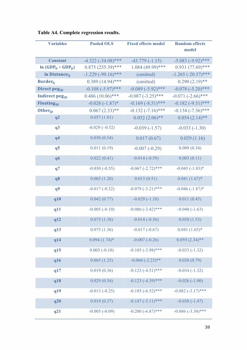
38    

Table A4. Complete regression results.

Variables Pooled OLS Fixed effects model Random effects model

Constant -4.322 (-34.08)*** -43.779 (-1.15) -5.083 (-9.92)*** ln (𝐆𝐃𝐏𝐢𝐭 ∗ 𝐆𝐃𝐏𝐣𝐭) 0.875 (255.39)*** 1.084 (49.99)*** 0.931 (77.69)***

ln 𝐃𝐢𝐬𝐭𝐚𝐧𝐜𝐞𝐢𝐣 -1.229 (-99.16)*** (omitted) -1.265 (-20.57)*** 𝐁𝐨𝐫𝐝𝐞𝐫𝐢𝐣 0.389 (14.94)*** (omitted) 0.290 (2.19)** 𝐃𝐢𝐫𝐞𝐜𝐭  𝐩𝐞𝐠𝐢𝐣𝐭 -0.108 (-5.97)*** -0.089 (-5.92)*** -0.078 (-5.20)*** 𝐈𝐧𝐝𝐢𝐫𝐞𝐜𝐭  𝐩𝐞𝐠𝐢𝐣𝐭 0.486 (10.06)*** -0.087 (-3.25)*** -0.071 (-2.66)*** 𝐅𝐥𝐨𝐚𝐭𝐢𝐧𝐠𝐢𝐣𝐭 -0.026 (-1.87)* -0.169 (-8.51)*** -0.182 (-9.51)*** 𝐎𝐭𝐡𝐞𝐫𝐢𝐣𝐭 0.067 (2.33)** -0.132 (-7.16)*** -0.134 (-7.36)***

q2 0.057 (1.01) 0.052 (2.06)** 0.054 (2.14)**

q3 -0.029 (–0.52) -0.039 (-1.57) -0.033 (-1.30)

q4 0.030 (0.54) 0.017 (0.67) 0.029 (1.16)

q5 0.011 (0.19) -0.007 (-0.29) 0.009 (0.34)

q6 0.022 (0.41) -0.014 (-0.59) 0.003 (0.11)

q7 -0.030 (-0.55) -0.067 (-2.72)*** -0.045 (-1.83)*

q8 0.065 (1.20) 0.013 (0.51) 0.041 (1.67)*

q9 -0.017 (-0.32) -0.079 (-3.21)*** -0.046 (-1.87)*

q10 0.042 (0.77) -0.029 (-1.18) 0.011 (0.45)

q11 -0.005 (-0.10) -0.086 (-3.42)*** -0.040 (-1.63)

q12 0.075 (1.38) -0.014 (-0.56) 0.038 (1.53)

q13 0.075 (1.36) -0.017 (-0.67) 0.041 (1.65)*

q14 0.094 (1.74)* -0.007 (-0.26) 0.059 (2.34)**

q15 0.005 (-0.10) -0.105 (-3.98)*** -0.033 (-1.32)

q16 0.065 (1.25) -0.060 (-2.23)** 0.020 (0.79)

q17 0.019 (0.36) -0.123 (-4.51)*** -0.034 (-1.32)

q18 0.029 (0.54) -0.123 (-4.39)*** -0.026 (-1.00)

q19 -0.013 (-0.25) -0.185 (-6.52)*** -0.082 (-3.17)***

q20 0.019 (0.37) -0.147 (-5.11)*** -0.038 (-1.47)

q21 -0.005 (-0.09) -0.200 (-6.87)*** -0.086 (-3.30)***

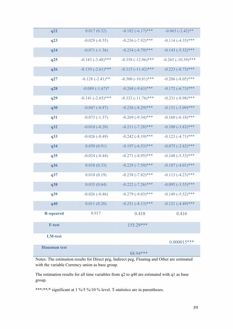
39    

q22 0.017 (0.32) -0.182 (-6.17)*** -0.063 (-2.42)**

q23 -0.029 (-0.55) -0.236 (-7.92)*** -0.114 (-4.35)***

q24 -0.071 (-1.36) -0.254 (-8.79)*** -0.143 (-5.52)***

q25 -0.183 (-3.48)*** -0.358 (-12.96)*** -0.265 (-10.39)***

q26 -0.139 (-2.61)*** -0.315 (-11.42)*** -0.223 (-8.73)***

q27 -0.128 (-2.41)** -0.300 (-10.81)*** -0.206 (-8.05)***

q28 -0.089 (-1.67)* -0.268 (-9.63)*** -0.172 (-6.73)***

q29 -0.141 (-2.65)*** -0.332 (-11.76)*** -0.231 (-8.98)***

q30 -0.047 (-0.87) -0.236 (-8.29)*** -0.131 (-5.09)***

q31 -0.073 (-1.37) -0.269 (-9.34)*** -0.160 (-6.18)***

q32 -0.010 (-0.20) -0.211 (-7.28)*** -0.100 (-3.83)***

q33 -0.026 (-0.49) -0.242 (-8.19)*** -0.123 (-4.71)***

q34 0.050 (0.91) -0.197 (-6.53)*** -0.075 (-2.82)***

q35 -0.024 (-0.44) -0.271 (-8.95)*** -0.148 (-5.53)***

q36 0.018 (0.33) -0.229 (-7.59)*** -0.107 (-4.01)***

q37 0.010 (0.19) -0.238 (-7.82)*** -0.113 (-4.23)***

q38 0.035 (0.64) -0.222 (-7.26)*** -0.095 (-3.55)***

q39 -0.026 (-0.46) -0.279 (-9.03)*** -0.149 (-5.52)***

q40 0.011 (0.20) -0.251 (-8.13)*** -0.121 (-4.49)***

R-squared 0.917 0.418

0.416

F-test 155.29***

LM-test 0.000015***

Hausman test 88.94***

Notes: The estimation results for Direct peg, Indirect peg, Floating and Other are estimated with the variable Currency union as base group.

The estimation results for all time variables from q2 to q40 are estimated with q1 as base group.

***/**/* significant at 1 %/5 %/10 % level. T-statistics are in parentheses.

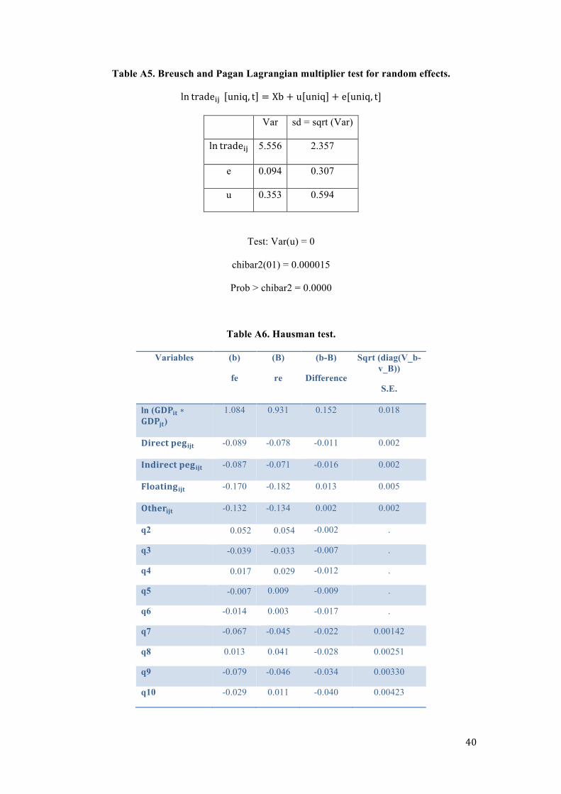
40    

Table A5. Breusch and Pagan Lagrangian multiplier test for random effects.

ln trade!"   uniq, t = Xb + u uniq + e[uniq, t]

Var sd = sqrt (Var)

ln trade!" 5.556 2.357

e 0.094 0.307

u 0.353 0.594

Test: Var(u) = 0

chibar2(01) = 0.000015

Prob > chibar2 = 0.0000

Table A6. Hausman test.

Variables (b)

fe

(B)

re

(b-B)

Difference

Sqrt (diag(V_b-v_B))

S.E.

ln (𝐆𝐃𝐏𝐢𝐭 ∗𝐆𝐃𝐏𝐣𝐭)

1.084 0.931 0.152 0.018

𝐃𝐢𝐫𝐞𝐜𝐭  𝐩𝐞𝐠𝐢𝐣𝐭 -0.089 -0.078 -0.011 0.002

𝐈𝐧𝐝𝐢𝐫𝐞𝐜𝐭  𝐩𝐞𝐠𝐢𝐣𝐭 -0.087 -0.071 -0.016 0.002

𝐅𝐥𝐨𝐚𝐭𝐢𝐧𝐠𝐢𝐣𝐭 -0.170 -0.182 0.013 0.005

𝐎𝐭𝐡𝐞𝐫𝐢𝐣𝐭 -0.132 -0.134 0.002 0.002

q2 0.052 0.054 -0.002 .

q3 -0.039 -0.033 -0.007 .

q4 0.017 0.029 -0.012 .

q5 -0.007 0.009 -0.009 .

q6 -0.014 0.003 -0.017 .

q7 -0.067 -0.045 -0.022 0.00142

q8 0.013 0.041 -0.028 0.00251

q9 -0.079 -0.046 -0.034 0.00330

q10 -0.029 0.011 -0.040 0.00423

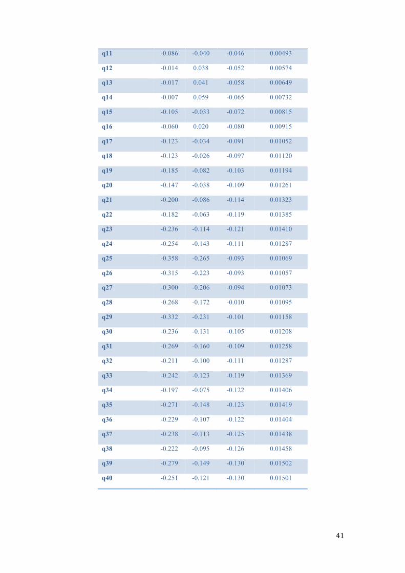
41    

q11 -0.086 -0.040 -0.046 0.00493

q12 -0.014 0.038 -0.052 0.00574

q13 -0.017 0.041 -0.058 0.00649

q14 -0.007 0.059 -0.065 0.00732

q15 -0.105 -0.033 -0.072 0.00815

q16 -0.060 0.020 -0.080 0.00915

q17 -0.123 -0.034 -0.091 0.01052

q18 -0.123 -0.026 -0.097 0.01120

q19 -0.185 -0.082 -0.103 0.01194

q20 -0.147 -0.038 -0.109 0.01261

q21 -0.200 -0.086 -0.114 0.01323

q22 -0.182 -0.063 -0.119 0.01385

q23 -0.236 -0.114 -0.121 0.01410

q24 -0.254 -0.143 -0.111 0.01287

q25 -0.358 -0.265 -0.093 0.01069

q26 -0.315 -0.223 -0.093 0.01057

q27 -0.300 -0.206 -0.094 0.01073

q28 -0.268 -0.172 -0.010 0.01095

q29 -0.332 -0.231 -0.101 0.01158

q30 -0.236 -0.131 -0.105 0.01208

q31 -0.269 -0.160 -0.109 0.01258

q32 -0.211 -0.100 -0.111 0.01287

q33 -0.242 -0.123 -0.119 0.01369

q34 -0.197 -0.075 -0.122 0.01406

q35 -0.271 -0.148 -0.123 0.01419

q36 -0.229 -0.107 -0.122 0.01404

q37 -0.238 -0.113 -0.125 0.01438

q38 -0.222 -0.095 -0.126 0.01458

q39 -0.279 -0.149 -0.130 0.01502

q40 -0.251 -0.121 -0.130 0.01501

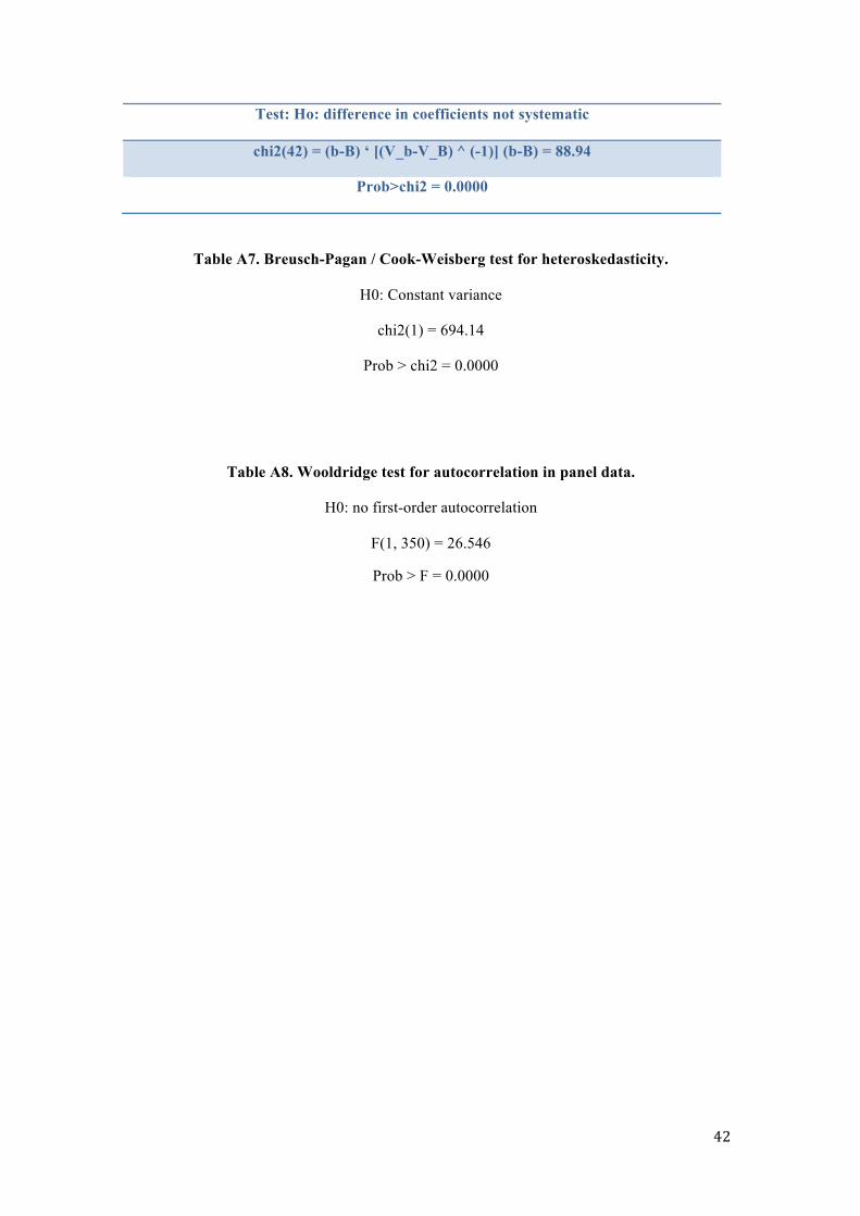
42    

Test: Ho: difference in coefficients not systematic

chi2(42) = (b-B) ‘ [(V_b-V_B)  ^ (-1)] (b-B) = 88.94

Prob>chi2 = 0.0000

Table A7. Breusch-Pagan / Cook-Weisberg test for heteroskedasticity.

H0: Constant variance

chi2(1) = 694.14

Prob > chi2 = 0.0000

Table A8. Wooldridge test for autocorrelation in panel data.

H0: no first-order autocorrelation

F(1, 350) = 26.546

Prob > F = 0.0000