Anticipating species distributions: handling1

sampling effort bias under a Bayesian2

framework3

Duccio Rocchini 1,*, Carol X. Garzon-Lopez 2, Matteo4

Marcantonio 1,3,*, Valerio Amici4, Giovanni Bacaro5, Lucy5

Bastin6,7, Neil Brummitt8, Alessandro Chiarucci9, Giles M.6

Foody10, Heidi C. Hauffe1, Kate S. He11, Carlo Ricotta12,7

Annapaola Rizzoli1, Roberto Rosa18

December 2, 20169

1 Fondazione Edmund Mach, Research and Innovation Centre, Department10

of Biodiversity and Molecular Ecology, Via E. Mach 1, 38010 S. Michele11

all’Adige (TN), Italy, corresponding author: ducciorocchini@gmail.com, duc-12

cio.rocchini@fmach.it13

2 UR “Ecologie et Dynamique des Systemes Anthropises” (EDYSAN, FRE14

3498 CNRS), 9 Universite de Picardie Jules Verne, 1 rue des Louvels, FR-15

80037 Amiens Cedex 1, France; 216

3 Department of Pathology, Microbiology, and Immunology, School of Vet-17

erinary Medicine, University of California, Davis, USA18

4 Department of Life Sciences, Universitfy of Siena, Via P.A. Mattioli 4,19

53100 Siena, Italy20

5 Department of Life Sciences, University of Trieste, Via L. Giorgieri 10,21

34127 Trieste, Italy22

6 School of Computer Science, Aston University, UK23

7 Currently on secondment to Joint Research Centre of the European Com-24

mission25

8 Department of Life Sciences, Natural History Museum, Cromwell Road,26

London, SW7 5BD, UK27

1

© 2017, Elsevier. Licensed under the Creative Commons Attribution-NonCommercial-NoDerivatives 4.0 Internationalhttp://creativecommons.org/licenses/by-nc-nd/4.0/

*Graphical Abstract

9 BIGEA, Department of Biological, Geological and Environmental Sciences,28

Alma Mater Studiorum, University of Bologna, Via Irnerio 42, 40126, Bologna,29

Italy30

10 University of Nottinhgam, University Park, Nottingham, NG7 2RD, UK31

11 Department of Biological Sciences, Murray State University, Murray, Ken-32

tucky, 42071, USA33

12 Department of Environmental Biology, University of Rome “La Sapienza”,34

00185 Rome, Italy35

∗ Authors contributed equally to the paper36

Abstract37

Anticipating species distributions in space and time is necessary for38

effective biodiversity conservation and for prioritising management in-39

terventions. This is especially true when considering invasive species.40

In such a case, anticipating their spread is important to effectively plan41

management actions. However, considering uncertainty in the output42

of species distribution models is critical for correctly interpreting re-43

sults and avoiding inappropriate decision-making. In particular, when44

dealing with species inventories, the bias resulting from sampling effort45

may lead to an over- or under-estimation of the local density of occur-46

rences of a species. In this paper we propose an innovative method to47

i) map sampling effort bias using cartogram models and ii) explicitly48

consider such uncertainty in the modeling procedure under a Bayesian49

framework, which allows the integration of multilevel input data with50

prior information to improve the anticipation species distributions.51

52

Keywords: anticipation, Bayesian theorem, sampling effort bias,53

Species Distribution Modeling, uncertainty54

55

List of acronyms: DIC: Deviance Information Criterion, MCMC:56

Markov Chain Monte Carlo, PPD: posterior probability distribution,57

SDM: Species Distribution Models58

1 Introduction59

Anticipation is an important topic in ecological fields such as food science60

(Lobell et al., 2012), community ecology (Keddy, 1992), species distribution61

modeling (Willis et al., 2009), landscape ecology (Tattoni et al., in press),62

and biological invasion science (Rocchini et al., 2015). Anticipatory methods63

2

are also crucial for developing effective management practices to deal with64

invasive species (Rocchini et al., 2015).65

Invasive species can modify the structure and functioning of ecosystems,66

altering biotic interactions and homogenizing previously diverse plant and67

animal communities over large spatial scales, ultimately resulting in a loss of68

genetic, species and ecosystem diversity (Winter et al., 2009). The annual69

economic impact of invasive species has been estimated at over 100 billion70

dollars just within the USA (NRC, 2002), an order of magnitude higher than71

those caused by all natural disasters put together (Ricciardi et al., 2011);72

some authors go as far as to claim that the economic impact of invasive73

species is incalculable (Mack et al., 2000).74

Given the massive negative economic and ecological effects of invasive75

species, a robust method for predicting species’ distributions is crucial for an76

early assessment of species invasions and effective application of appropriate77

management actions (Malanson and Walsh, 2013).78

Investigating how biodiversity is distributed spatially and temporally79

across the globe has long been a central theme in ecology (Gaston, 2000)80

and the methods developed to answer this question have become key tools for81

biodiversity monitoring (Ferretti and Chiarucci, 2003). For example, species82

distribution models (SDMs) have been used to map the current distribution83

of a single species (Rocchini et al., 2011), model the potential distribution84

of native and invasive species (Rocchini et al., 2015), investigate the sta-85

tistical performance of different models to infer the distribution of species86

under various ecological conditions (Guisan and Zimmermann, 2000; Elith87

and Graham, 2009), test the transferability in space of modeled distribu-88

tion patterns (Randin et al., 2006; Heikkinen et al., 2012), predict long term89

changes to species distributions (Pearman et al., 2008) and make inferences90

on future biodiversity scenarios (Pompe et al., 2008; Engler et al., 2009),91

evaluate the potential of satellite imagery bands as predictors of biodiver-92

sity patterns (Mathys et al., 2009), analyse spatial autocorrelation in species93

distributions (Carl and Kuhn, 2007; Dormann, 2007), and understand bio-94

geographical patterns (Sax, 2001).95

In combination with remote sensing products (e.g. Rocchini (2007); Feil-96

hauer et al. (2013)) and current global data sets on in situ species observa-97

tions, SDMs have become the method of choice for monitoring biodiversity at98

multiple spatial and temporal scales. However, the strength of this combina-99

tion depends on the careful selection and application of integrative modeling100

approaches, in combination with a thorough assessment of uncertainty in101

both data inputs and modeling methods.102

Reliable anticipation of species invasions depends on the quality of input103

data on one hand and robustness of the predictive SDM on the other. As104

3

an example, Rocchini et al. (2011) demonstrated theoretically that input105

data arising from biased species distribution maps could potentially lead to106

unsuitable management strategies. In addition, Elith and Leathwick (2009)107

demonstrated that, given the same input data set, different SDMs might108

lead to dissimilar results (see also Bierman et al. (2010); Manceur and Kuhn109

(2014)).110

The aim of this manuscript is to propose coherent and straightforward111

methods to explicitly account for uncertainty when mapping species distribu-112

tions in the light of anticipating the spread of invasive species. In particular113

we will cover: i) explicitly mapping uncertainty in sampling bias, ii) mitigat-114

ing uncertainty in data through prior beliefs and Bayesian inference and iii)115

reporting uncertainty in species distribution maps through Markov Chain116

Monte Carlo methods. The findings of this manuscript should be of par-117

ticular interest to landscape managers and planners attempting to predict118

the spread of species and deal with errors in species distribution maps in a119

straightforward manner.120

2 Mapping input uncertainty related to sam-121

pling effort bias122

In anticipating species distributions a first step is to ensure that the infor-123

mation indicating where species are present is bias-free or, at least, that the124

uncertainty of input data is explicitly taken into account in further modeling125

steps.126

One of the main problems with field data on species distributions is re-127

lated to “sampling effort bias” (Rocchini et al., 2011), namely the bias inher-128

ent in some areas being under-sampled with respect to others. Quantifying129

and mapping the uncertainty derived from variation in the number of obser-130

vations due to sampling effort can be achieved using cartograms (Gastner and131

Newman, 2004), in which the shape of spatial objects (e.g. polygons, cells,132

etc.) is directly related to a determined property, in our case to uncertainty.133

Cartograms build on the standard treatment of diffusion theory by Gast-ner and Newman (2004), in which the current spatial density of a populationis given by:

J = v(r, t)p(r, t) (1)

where v(r, t) and p(r, t) are the velocity and density of the spread of the134

population under study, respectively, at position r and time t.135

Cartograms facilitate the visualization of spatial uncertainty in the data136

4

by varying the size of each polygon according to the density of information137

contained (e.g. number of observations, variation, etc.). As an example,138

we show a cartogram of the distribution of Abies alba Miller overlapping a139

grid to the set of records obtained from the Global Biodiversity Information140

Facility (GBIF, http://www.gbif.org, Figure 1). GBIF offers free and open141

access to hundreds of millions of records from over 30,000 species datasets142

which are collated from around the world and stored with a common Darwin143

Core data standard. The cartogram was developed using the free and open144

source software ScapeToad (http://scapetoad.choros.ch/). Since cells with a145

higher number species occurrences might be biased by the effort spent visit-146

ing them, in Figure 1, the shape of each cell is determined by the the number147

of times it was visited (i.e. number of different dates recorded in GBIF for148

the species in that cell). From now on, we will refer to this as sampling effort.149

The colour represents the spatial distribution (density of occurrences, sensu150

) of the species in each cell.151

Therefore, cartograms allow uncertainty to be shown explicitly in a straight-152

forward manner. Furthermore, sampling effort might be considered as a153

variable in the SDM procedure, as described in the next section.154

3 Accounting for input uncertainty in the mod-155

eling procedure: multi-level models, prior156

beliefs and probability distribution surfaces157

Species observation records are often heterogeneous and incomplete because,158

for example, they are unevenly distributed by year or area, or were collected159

by different field operators. In addition, there is wide variation in recording160

behaviours.161

GBIF is a classic example of such heterogeneity: GBIF data is oppor-162

tunistically gathered from a mixture of systematic surveys and volunteer163

projects, and the intensity of publishing effort is strongly influenced by the164

membership of the organisation. In terms of geographic coverage, GBIF con-165

tains plentiful data from Northern Europe and America, parts of Latin and166

Central America, South Africa, Australia and Oceania – but by contrast,167

there are significant gaps in other regions, and there is a large variation168

in sampling effort even between neighbouring European countries (see Ap-169

pendix 1, Figure S1). This heterogeneity makes it difficult to estimate the170

underlying variable (actual species presence and density of occurrences) and171

potentially has an enormous impact on the information content of any one172

species observation or set of observations (Isaac and Pocock, 2015). This173

5

paper proposes methods by which ancillary knowledge about a species and174

its environment might be exploited in a Bayesian framework to increase that175

information content.176

Multi-level models can be essential for detecting (spatially) clustered data177

by considering the variation between groups (clusters). This approach is178

more efficient and powerful than standard linear modeling techniques as it179

provides a coherent and flexible method for modeling the effects of sampling180

variation and allows uncertainty to be elegantly accounted for at all levels of181

data structure (Gelman and Hill, 2006).182

Furthermore, environmental variables with different spatial or temporal183

resolution (i.e., country, regional or pixel level) are often used as predictors184

in SDMs. Multi-levels models can simultaneously and coherently incorpo-185

rate multi-level predictors allowing effects to be modelled at the appropriate186

scale (Gelman and Hill, 2006). Hierarchical models are naturally handled187

using Bayesian methods, which provide intuitive and direct estimates of un-188

certainty around parameter estimates (Link et Sauer, 2002).189

Despite tremendous effort by ecologists, collecting unbiased and reliable190

data on the presence of species in a determined area/time to assess their191

potential distribution through SDMs is sometimes not feasible since system-192

atic field work is inherently expensive, time-consuming, and often involves193

logistical hurdles, if the species under study is, for example, rare, elusive, in-194

habits remote areas, or is in transitional equilibrium with its ecological niche195

(as is the case with invasive species). Even for less problematic species, pres-196

ence/absence data may also be distorted by several potential flaws, such as197

sampling errors and subjectivity. As a result, SDM outputs may show high198

uncertainty and be difficult to interpret, jeopardizing their utility in con-199

servation applications. However, besides the availability of observation data200

directly exploitable for modeling purposes, there is a wider set of ecological201

data that can be used in SDMs, the so called “prior knowledge”. This data202

is very often neglected and comprises information represented in different203

formats; for example, previously conducted experiments, scientific literature204

on the studied species or similar species, or even as “prior beliefs” (basic eco-205

logical principles). Bayesian inference allows basic ecological principles and206

prior data to be incorporated in a straightforward manner with potential207

cost-effective consequences in increasing confidence of SDMs (McCarthy and208

Masters, 2005; Bierman et al., 2010; Manceur and Kuhn, 2014). The prior209

information needs to be translated into a probability distribution, which is210

then combined under Bayes’ rule with the likelihood information contained in211

the original data to estimate a “posterior belief” or posterior probability dis-212

tribution (PPD). The contribution of the prior and the data to the posterior213

distribution depends on their relative precision, with the more precise of the214

6

two having the greatest effect. A prior distribution can be non-informative215

(flat prior), mildly informative (vague prior) or informative (strong prior).216

In any case, the prior must be clearly described and justified according to217

the context under investigation (Kruschke, 2015).218

The result of the interaction between the likelihood of the data and the219

prior distribution is itself a probability distribution (posterior probability220

distribution or PPD). In an SDM, the advantage of having model parameter221

estimations expressed as probability distributions, and not as point estima-222

tion of the mean, is that the predicted suitability of the species in each223

prediction unit (pixel) is itself a probability distribution. The suitability of224

the PPD in each spatial unit represents the uncertainty of the prediction225

in that unit. This uncertainty is stored in the Markov Chain Monte Carlo226

(MCMC) model and can be re-used in future modeling exercises that, for227

example, use a different set of data.228

As an example, we applied a multi-level logistic regression with Bayesian229

inference to model the distribution of Abies alba in Europe. We chose this230

species due to its well known autoecology and actual distribution in Europe231

(Farjon, 1998; Tinner et al., 2013; Gazol et al., 2015). We derived 44375232

Abies alba presence records from the GBIF database, as points in vector233

format (see Appendix 1, Figures S3 and S4). We generated an equal number234

of pseudoabsences using the following strategy: we selected random points235

a) within areas where conifers have been sampled (conifer occurrences in236

the GBIF dataset) to pick the same areas that have been surveyed using the237

sampling protocol used to record Abies alba presences, b) outside dry climatic238

zones (e.g. Mediterranean climate) derived from the Koppen-Geiger climatic239

zones map (Koppen and Geiger, 1930) where this species is not found and c)240

outside a radius of 100 metres around the presence points to avoid overlap241

with presence points.242

We generated an equal number of absence locations at areas within which243

conifers have been sampled (conifer occurrences in the GBIF dataset) and244

outside a 100 meters radius from the presence points and the temperate and245

dry climatic zones (e.g. mediterranean climate) derived from the Koppen-246

Geiger climatic zones map .247

To select the predictor variables, we performed a literature review on248

the ecology of the species (Aussenac, 2002; Wolf, 2003; Rolland et al., 2009;249

Tinner et al., 2013; Gazol et al., 2015). Hence, we relied on three different250

datasets by selecting: i) the annual mean temperature (Bio1), and mean251

diurnal temperature range (Bio2) obtained from the WorldClim dataset (Hi-252

jmans et al., 2005), ii) radiation seasonality (Bio23) and the annual mean253

moisture index (Bio28), obtained from the CliMond dataset (Kriticos et al.,254

2012), and iii) the number of wet days during summer and frost days during255

7

winter (and early spring) derived from the wet-days and ground-frost data256

in the climate research unit dataset (Mitchell et al., 2004) (see Figure 2).257

258

Considering sampling effort as a predictor, the sampling of the GBIF259

dataset is clearly opportunistic. As a result, the unevenness of sampling260

effort is particularly evident, with the Northern European region being more261

sampled than other European regions (see Appendix 1, Figure S1). This bias262

in GBIF data could generate unreliable predictions.263

The clustering of GBIF data mainly derives from differences in surveys at264

national and subnational level (Appendix 1, Figure S1). Thus, the sampling265

effort was derived as the number (richness) of dates of survey recorded in the266

GBIF dataset per polygon of the official administrative division of European267

countries using the Nomenclature of Territorial Units for Statistics level 3268

(NUTS 3).269

We built a multi-level model to take into account the different resolution270

of the predictor variables (Figure 2) and the differential sampling effort of271

Abies alba occurrences in each NUTS3 polygon. The sampling effort was272

used to re-scale the precision of the likelihood at pixel level, multiplying the273

scaled sampling effort by the standard deviation of the Gaussian likelihood.274

As a result, the likelihood estimate of pixels in regions with a higher number275

of samples was expected to be more precise. The theoretical model (Figure276

2) was coded in JAGS language and run in JAGS 4.2.0 through R (R Core277

Team, 2016) using the R2jags (Su and Yajima, 2016) and CODA (Plummer278

et al., 2002) packages. In order to allow reproducibility (Rocchini and Neteler279

(2012)) of our approach we have included the complete R code in Appendix280

2.281

As previously stated, in heterogeneous datasets like the GBIF set, thesampling effort in a certain region may be correlated with the presence ofthe species under study. Therefore, a more highly sampled region should havealso a higher probability of hosting the species. However, our data showed aweak sampling effort signal, with a high number of very low-sampled regionsshowing presence of Abies alba. This may result from errors, or low numbersof records not being representative of the distribution of the species understudy. Therefore, we applied uninformative priors (µ = 0, SD = 1/10−2) forall the predictors but not for sampling effort, whose prior distribution p(θ)was given three different sets of parameters:

p(θ) =

dnorm(0, 1/10−2), uninformative prior.

dnorm(1, 10), mild positive prior.

dnorm(5, 5), strong positive prior.

(2)

282

8

Such distributions were chosen as examples under the hypothesis that i)283

data alone were enough to account for heterogeneity in sampling effort; ii)284

a mildly informative (vague) prior knowledge about the positive correlation285

of sampling effort was useful for improving the model; iii) imposing strong286

prior knowledge on the positive influence of the prior would improve the287

model output. These three hyphoteses were translated in three models that288

shared the same structure (Figure 2) exept for the prior distribution imposed289

on sampling effort. All the predictors were scaled and centered in order to290

improve the efficiency of the MCMC process. PPDs for all parameters were291

sampled from each of two chains with 10000 MCMC iterations using 1000292

burn-in and 1000 adaptation iterations, with a thinning set of 20. Conver-293

gence was assesed by the Gelman-Rubin statistic (Gelman and Rubin, 1992).294

Each model was then used to estimate the suitability PPDs in each pixel of295

the study area. The parameter estimates for the three models will show if296

different prior belief on the role of sampling effort changed the model pa-297

rameter estimates. Furthermore, the Deviance Information Criterion (DIC,298

see Spiegelhalter et al. (2014)) was used to assess the model with the best299

predictive power.300

The Posterior Probability Distributions (PPDs) of model parameters for301

the three models (with different priors on sampling effort, see Equation 2)302

are reported in Figure 3. All the models agreed on the direction and effect303

size of the predictors (Figure 3). Credible effects (no intersection with 0 in304

Figure 3) were attained for those variables directly related to temperature. In305

particular, annual mean temperature (Bio1 and Bio12) and radiation season-306

ality (Bio23) showed negative effects while mean diurnal temperature range307

(Bio2) showed positive effects (Figures 3 and 4). The negative credible effect308

of Bio12 implies that the relationship between the probability of presence309

(suitability) of Abies alba and annual mean temperature has a “bell shape”,310

by rising slowly to the left of the annual mean temperature average (7.8 °C)311

and decreasing rapidly when on its right (Figure 4). On the contrary, the312

distribution of wet days, annual mean moisture index (Bio28) and frost days313

included 0, showing a non-credible effect on the presence of Abies alba.314

The sampling effort coefficient changed heavily between models. In the315

first model with an uninformative prior, the coefficient average was slightly316

negative but with its high density interval comprising 0 (Figure 3). Therefore317

we concluded that according to the data the sampling effort had a non-318

credible effect. In the second model (Figure 3) a mildly informative positive319

prior affected the estimate of the parameters, but yet was not enough to320

derive a credible effect of the prior estimate. In the last model, the strong321

informative prior pulled the estimation of sampling effort coefficient towards322

positive values. This showed that, according to the data and to the “prior323

9

knowledge”, the sampling effort was positively affecting the probability of324

presence of Abies alba.325

In summary, the model with the strong prior showed an improved preci-326

sion of sampling effort, basically maintaining that of the others (Figure 3).327

Based on this and since the DIC did not show differences for the strong prior-328

model with respect to the uninformative prior-model (Table 1, δDIC ≤ 4,329

see Burnham and Anderson (2002)), we further focused on the model with330

a strong prior to build the output distribution map. The resulting potential331

niche distribution of Abies alba is thus shown in Figure 5.332

4 Discussion333

In this paper, we have demonstrated the importance of i) mapping uncer-334

tainty derived from varying sampling effort and ii) considering it in an explicit335

manner in order to anticipate species’ potential distributions. We have pro-336

vided a case study with a plant species widespread throughout Europe (Abies337

alba) where the observed data (Figure 1) and the modelled potential niche338

(Figure 5) differed mainly because of tree plantations recorded in the GBIF339

dataset. For example, Northern Europe was shown to be unsuitable for the340

natural spread of the species in our Bayesian model (Figure 5), as well as in341

previous studies on the distribution of the species (e.g. the European Forest342

genetic Resources programme, http://www.euforgen.org/, see Appendix 1,343

Figure S2), corroborating our results. However, it appeared to be present344

in the GBIF field-based dataset (Figure 1, see also Appendix 1, Figure S3),345

mainly because of human-related conifer plantations.346

Notably, when we associated a stronger prior to sampling effort, model347

coefficient estimates had lower uncertainty, and in addition, the model DIC348

did not differ from the model with the uninformative prior. Therefore, a349

strong prior allowed us to decrease uncertainty and maintain high model350

quality (δDIC ≤ 4, see Burnham and Anderson (2002)).351

We have shown that multilevel models coupled with Bayesian inference352

can be used to account for variability in sampling effort, integrating external353

data on prior knowledge with species observations, to model species distribu-354

tion more accurately and with higher certainty than previous methods. The355

priors considered in the reported case study were only examples generated356

here to illustrate how the precision of parameter estimates can potentially357

be increased using prior knowledge about the system under study. However,358

in order to have scientifically sound results, the priors considered should359

obviously be fully justified and rooted in ecological theory.360

Anticipating species potential distributions based on prior information361

10

(Bayesian modeling) can help to predict the potential future spread of a362

species in space (and time) in a robust manner (Bierman et al., 2010; Manceur363

and Kuhn, 2014). Using sampling effort bias among priors was important364

in our case since it allowed such uncertainty to be considered explicitly in365

the model. This can help to accommodate the error rate directly into the366

modeling procedure.367

Hence, calibrating models conditioned on previous knowledge and/or ob-368

servations might be feasible when relying on a Bayesian framework in which:369

P (Y |H) (3)

where P = the probability of occurrence of patterns Y given a hypothesis370

H is substituted by:371

P (H|Y ) (4)

i.e. the probability P that a hypothesis H is true in light of the available372

data.373

Bayesian statistics have long been used in independent scientific disci-374

plines and topics such as trait loci mapping (Ball, 2001), environmental sci-375

ence (Clark, 2005), machine learning approaches in computer science (Di-376

etterich, 2000), classification of remotely-sensed images (Goncalves et al.,377

2009), conservation genetics (Bertorelle et al., 2004), statistical algorithm378

development (Hoeting et al., 2009) and sampling strategies (Mara et al.,379

2016).380

In the framework of ecological patterns and processes, Ellison (2004)381

makes an explicit quest for using known information to build a model, re-382

lying on prior rather than posterior probabilities. This reinforces the view383

of Ginzburg et al. (2007) that biology should constrain mathematical con-384

structions. Quoting the authors, “While mathematics provides an incredibly385

vast set of possible equations, logic dictates that only a small subset of these386

equations can represent a given ecological phenomenon. A large number387

of constructions, while mathematically sound, should be excluded based on388

their inconsistency with biology.”389

This is especially true when the results of model construction impact390

decision-making, which could be more focused and effective if uncertainty391

was explicitly taken into account based on previous literature regarding the392

main drivers that shape the distribution of species (Ellison, 1996). Our393

approach reduces the danger of relying on misleading predictions of alien394

species invasions with high model errors, which are hidden or unrecognizable395

using previous approaches (Rocchini et al., 2015).396

11

In the framework of Species Distribution Modeling it has been demon-397

strated that prior probabilities in the observation of a certain species might398

improve model performance. This is true at various hierarchical levels, from399

species to entire communities. Thus, applying Bayes’ theorem to predict val-400

ues at a certain site might thus allow known environmental properties to be401

accounted for. If Bayesian models do not outperform other modeling tech-402

niques, they at least better reflect the theory under the realized niche of a403

certain species. A number of examples are provided in Guisan and Zimmer-404

mann (2000), modeling different plant species in different habitat types.405

5 Conclusion406

In the light of the importance of anticipating species future distributions,407

especially for economically important invasive species, it is crucial to detect408

those areas into which such a species might be expected to disperse. Antici-409

pating their spread based on the suitability of environmental conditions can410

lead to more effective management strategies, allowing timely actions to be411

initiated and preventing further spread (Rocchini et al., 2015).412

This can be summarized by the following equation:

Decision =

(< Em| > I < Em| < I> Em| > I > Em| < I

)(5)

In this case, a high (or low) invasion rate I might be related to high or413

low error Em in the output model being observed by decision makers. The414

most dangerous situation is when a low predicted invasion rate is related to415

a high error in the modeling procedure. In this case decision makers might416

underestimate the effort against the likelihood of invasion, that, from the417

species distribution map, is suspected to be low.418

In this paper we have demonstrated the power of incorporating sampling419

bias into the model being used by relying on prior probabilities of distribu-420

tion of a plant species widely spread in Europe. We believe this is a good421

example to further encourage species distribution modellers and environmen-422

tal planners and conservationists to account for uncertainty and bias in the423

sampling effort in anticipating the spatial spread of species, instead of relying424

on distribution maps with potentially hidden uncertainty.425

6 Acknowledgments426

We are particularly grateful to the handling Editor Rocco Scolozzi and to427

two anonymous Reviewers who provided useful insights which improved a428

12

first draft of this manuscript. We thank Ingolf Kuhn for precious sugges-429

tions.430

DR was partially supported by the EU BON (Building the European Biodi-431

versity Observation Network) project, funded by the European Union under432

the 7th Framework programme (Contract No. 308454), by the ERANET433

BioDiversa FP7 project DIARS, funded by the European Union and by the434

Life project Future For CoppiceS.435

References436

Alba-Sanchez, F., Lopez-Saez, J.A., Pando, B.B., Linares, J.C., Nieto-437

Lugilde, D., Lopez-Merino, L., 2010. Past and present potential distribu-438

tion of the Iberian Abies species: a phytogeographic approach using fossil439

pollen data and species distribution models. Diversity and Distributions440

16, 214–228. doi:10.1111/j.1472-4642.2010.00636.x441

Aussenac, G. (2002). Ecology and ecophysiology of circum-Mediterranean442

firs in the context of climate change. Annals of Forest Science 59: 823-832.443

Ball, RD. (2001). Bayesian Methods for Quantitative Trait Loci Mapping444

Based on Model Selection: Approximate Analysis Using the Bayesian In-445

formation Criterion.” Genetics, 159: 1351-1364.446

Barbosa, A., 2015. fuzzySim: applying fuzzy logic to binary similarity indices447

in ecology. Methods in Ecology and Evolution p. in press.448

Beck, J., Ballesteros-Mejia, L., Buchmann, C.M., Dengler, J., Fritz, S.A.,449

Gruber, B., Hof, C., Jansen, F., Knapp, S., Kreft, H., Schneider, A.-K.,450

Winter, M., Dormann, C.F. (2012). What’s on the Horizon for Macroecol-451

ogy? Ecography, 35: 673-683.452

Beck, J., Boller, M., Erhardt, A., Schwanghart, W. (2014). Spatial bias453

in the GBIF database and its effect on modeling species’ geographic454

distributions. Ecological Informatics, 19: 10-15.455

456

Bertorelle, G., Bruford, M., Chemini, C., Vernesi, C., Hauffe, H.C. (2004).457

New, flexible Bayesian approaches to revolutionize conservation genetics.458

Conservation Biology, 18: 1-2.459

Bierman, S.M., Butler, A., Marion, G., Kuhn, I. (2010). Bayesian image460

restoration models for combining expert knowledge on recording activity461

with species distribution data. Ecography, 33: 451-460.462

13

Burnham, K.P., Anderson, D.R., 2002. Model Selection and Multimodel463

Inference: A practical Information-Theoretic Approach, Second. ed.464

Springer.465

Carl, G., Kuhn, I. (2007). Analyzing spatial autocorrelation in species dis-466

tributions using Gaussian and logit models. Ecological Modelling, 207:467

159-170.468

Chen, G., Kery, M., Plattner, M., Ma, K., Gardner, B. (2012). Imperfect469

detection is the rule rather than the exception in plant distribution studies.470

Journal of Ecology, 101: 183-191.471

Clark, J. (2005) Why environmental scientists are becoming Bayesians. Ecol-472

ogy Letters, 8: 2-14.473

Dietterich, T.G. (2000). Ensemble Methods in Machine Learning. Lecture474

Notes in Computer Science, 1857: 1–15.475

Dormann, C.F. (2007). Effects of incorporating spatial autocorrelation into476

the analysis of species distribution data. Global Ecology and Biogeography,477

16: 129-138.478

Elith, J., Graham, C.H. (2009). Do they? How do they? WHY do they479

differ? On finding reasons for differing performances of species distribution480

models. Ecography, 32: 66-77.481

Elith, J., Leathwick, J.R. (2009) Species distribution models: ecological ex-482

planation and prediction across space and time. Annual Review of Ecology,483

Evolution, and Systematics, 40: 677-697.484

Ellison, A. (1996). An Introduction to Bayesian Inference for Ecological485

Research and Environmental Decision-Making. Ecological Applications 6:486

1036-1046.487

Ellison, A. (2004). Bayesian Inference in Ecology. Ecology Letters, 7: 509-488

520.489

Engler, R., Randin, C.F., Vittoz, P., Czaka, T., Beniston, M., Zimmermann,490

N.E., Guisan, A. (2009). Predicting future distributions of mountain plants491

under climate change: does dispersal capacity matter? Ecography, 32: 34-492

45.493

Farjon (1998), World Bibliography and Checklist of Conifers, RBG Kew.494

14

Feilhauer, H., Thonfeld, F., Faude, U., He, K.S., Rocchini, D., Schmidtlein,495

S. (2013). Assessing floristic composition with multispectral sensors - A496

comparison based on monotemporal and multiseasonal field spectra. Inter-497

national Journal of Applied Earth Observation and Geoinformation, 21:498

218-229.499

Ferretti, M., Chiarucci, A. (2003). Design concepts adopted in long-term500

forest monitoring programs in Europe - problems for the future? Science501

of The Total Environment, 310, 171-178.502

Gaston, K.J. (2000). Global patterns in biodiversity. Nature 405, 220-227.503

Gastner, M.T., Newman, M.E.J. (2004). Diffusion-based method for pro-504

ducing density-equalizing maps. Proceedings of the national Academy of505

Sciences USA, 101: 7499-7504.506

Gazol, A., Camarero, J.J., Gutierrez, E., Popa, I., Andreu-Hayles, L., Motta,507

R., Nola, P., Ribas, M., Sanguesa-Barreda, G., Urbinati, C., Carrer, M.508

(2015). Distinct effects of climate warming on populations of silver fir509

(Abies alba) across Europe. Journal of Biogeography, 42: 1150-1162.510

Gelman, A., Rubin, D.B. (1992). Inference from iterative simulation using511

multiple sequences. Statistical Science, 7: 457-511.512

Gelman, A., Hill, J. (2006). Data Analysis Using Regression and Multi-513

level/Hierarchical Models. Cambridge University Press.514

Ginzburg, L.R., Jensen, C.X.J., Yule, J.V. (2007). Aiming the “unreasonable515

effectiveness of mathematics” at ecological theory, Ecological Modelling,516

207, 356-362.517

Goncalves, Luisa, Cidalia Fonte, Eduardo Julio, and Mario Caetano. “A518

Method to Incorporate Uncertainty in the Classification of Remote Sensing519

Images.” International Journal of Remote Sensing 30, no. 20 (2009): 5503,520

5489.521

Guisan, A., Zimmermann, N.E. (2000). Predictive habitat distribution mod-522

els in ecology. Ecological Modelling, 135: 147-186.523

Heikkinen, R.K., Marmion, M., Luoto, M. (2012). Does the interpolation524

accuracy of species distribution models come at the expense of transfer-525

ability? Ecography 35: 276-288.526

15

Hijmans, R..J, Cameron, S.E., Parra, J.L., Jones, P.G., Jarvis, A. (2005)527

Very high resolution interpolated climate surfaces for global land areas.528

International Journal of Climatology, 25: 1965-1978.529

Hoeting, JA, CT Volinsky, and D Madigan. “Bayesian Model Averaging: A530

Tutorial.” Statistical Science 14, no. 4 (1999): 417, 382.531

Isaac, N.J.B., Pocock, M.J.O. (2015). Bias and information in biological532

records. Biological Journal of the Linnean Society, 115: 522-531.533

Keddy, P.A. (1992). Assembly and response rules: two goals for predictive534

community ecology. Journal of Vegetation Science 3: 157-164.535

Koppen, W., Geiger, R. (1930). Handbuch der klimatologie. Gebruder Born-536

traeger Berlin, Germany.537

Kriticos, D.J., Webber, B.L., Leriche, A., Ota, N., Bathols, J., Macadam, I.,538

Scott, J.K. (2012). CliMond: global high resolution historical and future539

scenario climate surfaces for bioclimatic modelling. Methods in Ecology540

and Evolution, 3: 53-64.541

Kruschke, J.K., 2015. Doing Bayesian Data Analysis, 2nd Edition, Elsevier,542

Amsterdam.543

Link, W.A., Sauer, J.R., 2002. A hierarchical analysis of population change544

with application to Cerulean Warblers. Ecology 83, 9.545

Lobell, D. B., Sibley, A., Ortiz-Monasterio, J.I. (2012). Extreme heat effects546

on wheat senescence in India. Nature Climate Change, 2: 186-189.547

Mack, R.N., Simberloff, D., Lonsdale, W.M., et al. (2000). Biotic invasions:548

causes, epidemiology, global consequences, and control. Ecological Appli-549

cations, 10: 689-710.550

Manceur, A.M., Kuhn, I. (2014). Inferring model-based probability of oc-551

currence from preferentially sampled data with uncertain absences using552

expert knowledge. Methods in Ecology and Evolution, 5: 739-750.553

Mathys, L., Guisan, A., Kellenberger, T.W., Zimmermann, N.E. (2009).554

Evaluating effects of spectral training data distribution on continuous field555

mapping performance. ISPRS Journal of Photogrammetry and Remote556

Sensing, 64: 665-673.557

16

Malanson, G.P., Walsh, S.J. (2013). A geographical approach to optimization558

of response to invasive species. In: Walsh SJ and Mena C (eds) Science559

and Conservation in the Galapagos Islands: Frameworks and Perspectives.560

New York, USA: Springer, pp. 199-215.561

Mara, T.A., Delay, F., Lehmann, F., Younes, A. (2016). A Comparison of562

Two Bayesian Approaches for Uncertainty Quantification. Environmental563

Modelling & Software, 82: 21-30.564

McCarthy, M.A., Masters, P., 2005. Profiting from prior information in565

Bayesian analyses of ecological data. Journal of Applied Ecology 42,566

1012–1019. doi:10.1111/j.1365-2664.2005.01101.x567

Mitchell, T.D., Carter, T.R., Jones, P.D., Hulme, M., New, M. (2004). A568

comprehensive set of climate scenarios for Europe and the globe: the ob-569

served record (1900-2000) and 16 scenarios (2000-2100). University of East570

Anglia, Norwich,UK, pp. 30.571

NRC (Committee on the Scientific Basis for Predicting the Invasive Potential572

of Non-indigenous Plants and Plant Pests in the United States) (2002)573

Predicting Invasions of Non-indigenous Plants and Plant Pests. Washing-574

ton, DC: National Academy Press.575

Pearman, P.B., Randin, C.F., Broennimann, O., Vittoz, P:, van der Knaap,576

W.O., Engler, R., Le Lay, G., Zimmermann, N.E., Guisan; A. (2008). Pre-577

diction of plant species distributions across six millennia. Ecology Letters,578

11: 357-369.579

Pompe, S., Hanspach, J., Badeck, F., Klotz, S., Thuiller, W., Kuhn, I. (2008).580

Climate and land use change impacts on plant distributions in Germany.581

Biology Letters, 4: 564-567.582

Plummer, M., Best, N., Cowles, K., Vines, K. (2006). CODA: Convergence583

Diagnosis and Output Analysis for MCMC. R News. 6: 7-11.584

R Core Team (2016). R: A language and environment for statistical com-585

puting. R Foundation for Statistical Computing, Vienna, Austria. URL586

http://www.R-project.org/.587

Randin, C.F., Dirnbock, T., Dullinger, S., Zimmermann, N.E., Zappa, M.,588

Guisan, A. (2006). Are niche-based species distribution models transferable589

in space? Journal of Biogeography, 33: 1689-1703.590

17

Ricciardi, A., Palmer M.E., Yan, N.D. (2011) Should biological invasions be591

managed as natural disasters? Bioscience, 61: 312-317.592

Rocchini, D. (2007). Distance decay in spectral space in analysing ecosystem593

b-diversity. International Journal of Remote Sensing, 28: 2635-2644.594

Rocchini, D., Andreo, V., Forster, M., Garzon-Lopez, C.X., Gutierrez, A.P.,595

Gillespie ,T.W., Hauffe, H.C., He, K.S., Kleinschmit, B., Mairota, P., Mar-596

cantonio, M., Metz, M., Nagendra, H., Pareeth, S., Ponti, L., Ricotta, C.,597

Rizzoli, A., Schaab, G., Zebisch, M., Zorer, R., Neteler, M. (2015). Poten-598

tial of remote sensing to predict species invasions - a modeling perspective.599

Progress in Physical Geography, 39: 283-309.600

Rocchini, D., Hortal, J., Lengyel, S., Lobo, J.M., Jimenez-Valverde, A., Ri-601

cotta, C., Bacaro, G., Chiarucci, A. (2011). Accounting for uncertainty602

when mapping species distributions: The need for maps of ignorance.603

Progress in Physical Geography, 35: 211-226.604

Rocchini, D., Neteler, M. (2012). Let the four freedoms paradigm apply to605

ecology. Trends in Ecology & Evolution, 27: 310–311.606

Rolland, C., Michalet, R., Desplanque, C., Petetin, A., Aime, S. 2009. Eco-607

logical requirements of Abies alba in the French Alps derived from dendro-608

ecological analysis. Journal of Vegetation Science, 10: 297-306.609

Sax, D.F. (2001). Latitudinal gradients and geographic ranges of exotic610

species: implications for biogeography. Journal of Biogeography, 28: 139-611

150.612

Spiegelhalter, D.J., Best, N.G., Carlin, B.P., van der Linde, A. (2014). The613

deviance information criterion: 12 years on (with discussion). Journal of614

the Royal Statistical Society, Series B, 76: 485-493.615

Su, Y.-S., Yajima, M. (2016). R2jags: A Package for Running jags from R.616

http://CRAN. R-project. org/package= R2jags617

Tattoni, C., Ianni, E., Geneletti, D., Zatelli, P., Ciolli, M. (in press). Land-618

scape changes, traditional ecological knowledge and future scenarios in the619

Alps: A holistic ecological approach. Science of the Total Environment.620

Tinner, W., Colombaroli, D., Heiri, O., Henne, P.D., Steinacher, M., Unte-621

necker, J., Vescovi, E., Allen, J.R.M., Carraro, G., Conedera, M., Joos,622

F., Lotter, A.F., Luterbacher, J., Samartin, S., Valsecchi, V. (2013). The623

past ecology of Abies alba provides new perspectives on future responses624

of silver fir forests to global warming. Ecological Monographs, 83: 419-439.625

18

Willis, S.G., Thomas, C., Hill, J.K., Collingham, Y., Telfer, M.G., Fox, R.,626

Huntley, B. (2009). Dynamic distribution modelling: predicting the present627

from the past. Ecography 32: 5-12.628

Winter, M., Schweiger, O., Klotz, S., Nentwig, W., Andriopoulos, P., Ari-629

anoutsou, M., Basnou, C., Delipetrou, P., Didziulis, V., Hejda, M., Hulme,630

P.E., Lambdon, J.P., Pysek, P., Royl, D.B., Ingolf Kuhn (2009). Plant631

extinctions and introductions lead to phylogenetic and taxonomic homog-632

enization of the European flora. Proceedings of the National Academy of633

Sciences of the United States of America, 106: 21721-21725.634

Wolf, H. (2003). EUFORGEN Technical Guidelines for genetic conservation635

and use for silver fir (Abies alba). International Plant Genetic Resources636

Institute, Rome, Italy. 6 pp.637

19

Tables638

Model DIC Gelman diagnostic Burn In Iterations ChainsUninformative prior 1938 1.13 2000 10000 2Mild prior 2133 1.15 2000 10000 2Strong prior 1940 1.22 2000 10000 2

Table 1: Deviance Information Criterion (DIC) used to assess the prior withthe best predictive power. Notice that δDIC ≤ 4 using an uninformativeprior and a strong prior on sampling effort. Therefore, a strong prior allowedus to decrease uncertainty and maintain high model quality. Refer to themain text for additional information.

20

Figures639

Figure 1: Cartogram representing the sampling effort bias (cell distortion) ofthe GBIF dataset related to Abies alba. This species is not native in NorthernEurope, although it is widely cultivated as a timber tree, as thus present inthe GBIF dataset.

21

Figure 2: The multi-level model represented through a pictogram. To selectthe predictor variables, we performed a literature review on the ecology ofthe species, finally selecting: radiation seasonality (Bio23), the annual meanmoisture index (Bio28), the number of wet days during summer and the frostdays during winter and early spring, the annual mean temperature (Bio1),the mean diurnal temperature range (Bio2). Sampling effort was calculatedas the richness of dates of survey recorded in the GBIF dataset for eachNUTS3 country. Refer to the main text for additional information on thesource of each dataset. Symbols used in this figure: µ, σ = mean and stan-dard deviation of prior and hyperprior distributions; ζ, χ, φ = intercepts forNUTS3, 35km, 6km level of the model; subscript d,j,i,o = index for NUTS3,35km, 6km and observation level; weightijd = scaled weights for sampling ef-fort; logistic(ψ) = logistic transformation of the model output (link function);pi|j|d = probability of occurrence; yo|i|j|d = presence or absence. Refer to Kr-uschke (2015) for a complete dissertation about the terms and the graphicalrepresentation of the proposed model. Notice that variables at 6km resolu-tion were resampled from an original resolution of 1km to allow the Bayesianmodel to be run in R. The R code of the model is available in Appendix 2.

22

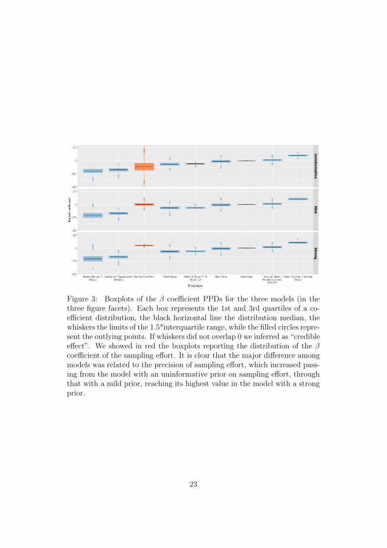
Figure 3: Boxplots of the β coefficient PPDs for the three models (in thethree figure facets). Each box represents the 1st and 3rd quartiles of a co-efficient distribution, the black horizontal line the distribution median, thewhiskers the limits of the 1.5*interquartile range, while the filled circles repre-sent the outlying points. If whiskers did not overlap 0 we inferred as “credibleeffect”. We showed in red the boxplots reporting the distribution of the βcoefficient of the sampling effort. It is clear that the major difference amongmodels was related to the precision of sampling effort, which increased pass-ing from the model with an uninformative prior on sampling effort, throughthat with a mild prior, reaching its highest value in the model with a strongprior.

23

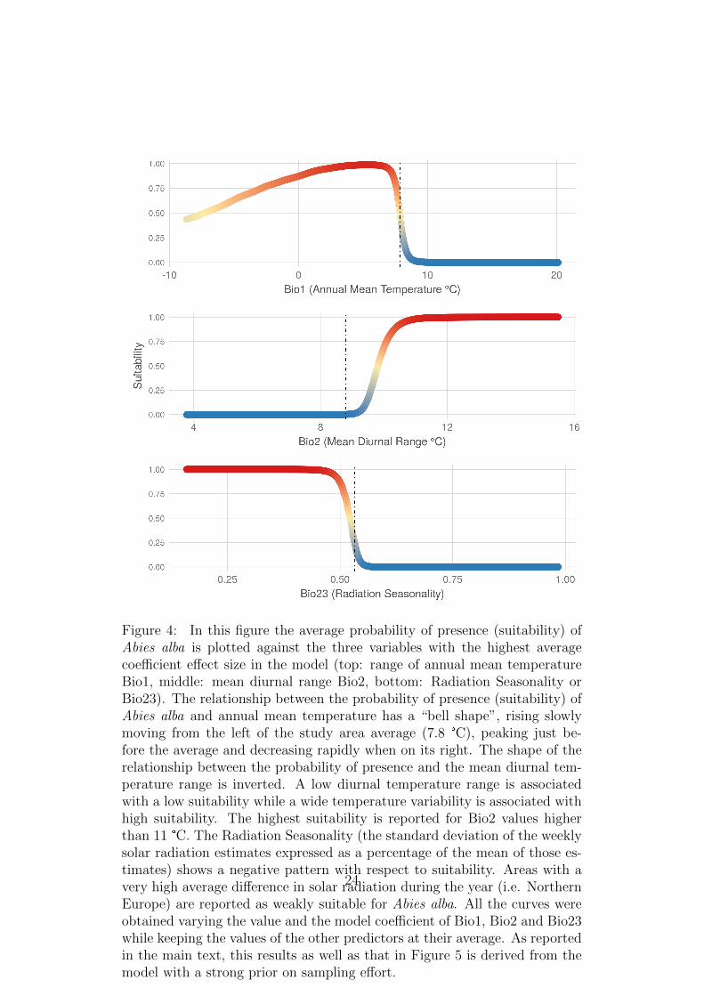
Figure 4: In this figure the average probability of presence (suitability) ofAbies alba is plotted against the three variables with the highest averagecoefficient effect size in the model (top: range of annual mean temperatureBio1, middle: mean diurnal range Bio2, bottom: Radiation Seasonality orBio23). The relationship between the probability of presence (suitability) ofAbies alba and annual mean temperature has a “bell shape”, rising slowlymoving from the left of the study area average (7.8 °C), peaking just be-fore the average and decreasing rapidly when on its right. The shape of therelationship between the probability of presence and the mean diurnal tem-perature range is inverted. A low diurnal temperature range is associatedwith a low suitability while a wide temperature variability is associated withhigh suitability. The highest suitability is reported for Bio2 values higherthan 11 °C. The Radiation Seasonality (the standard deviation of the weeklysolar radiation estimates expressed as a percentage of the mean of those es-timates) shows a negative pattern with respect to suitability. Areas with avery high average difference in solar radiation during the year (i.e. NorthernEurope) are reported as weakly suitable for Abies alba. All the curves wereobtained varying the value and the model coefficient of Bio1, Bio2 and Bio23while keeping the values of the other predictors at their average. As reportedin the main text, this results as well as that in Figure 5 is derived from themodel with a strong prior on sampling effort.

24

Figure 5: Abies alba suitability distribution as derived from the multi-levelmodel with strong prior on sampling effort. The pixel value is the average ofthe PPDs for that pixel.

25

Figure 1Click here to download high resolution image

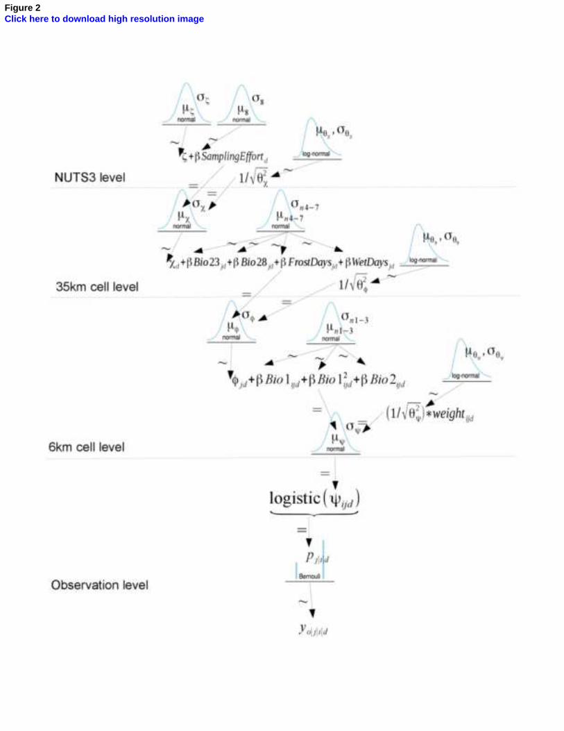
Figure 2Click here to download high resolution image

Figure 3Click here to download high resolution image

Figure 4Click here to download high resolution image

Figure 5Click here to download high resolution image

Figure S1Click here to download high resolution image

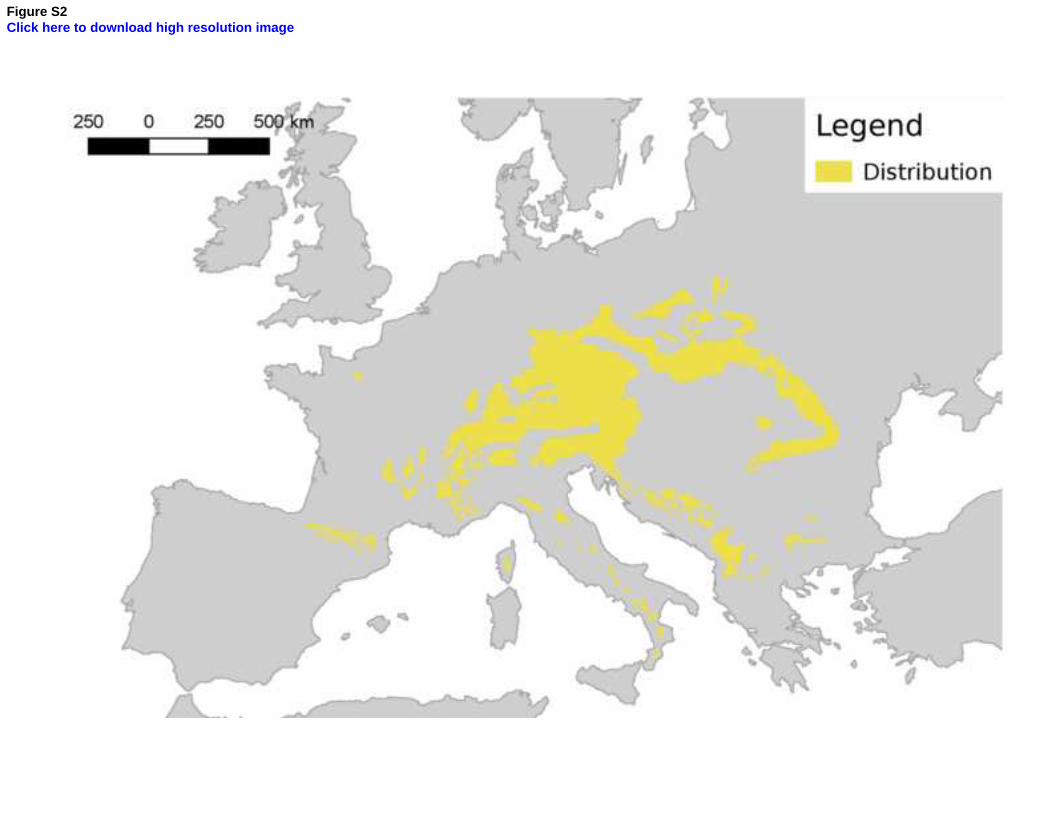
Figure S2Click here to download high resolution image

Figure S3Click here to download high resolution image

Figure S4Click here to download high resolution image