Anti-lock Braking System performance on rough terrain

Anti-lock Braking System performance on rough terrain

Wietsche Clement William Penny

Submitted in partial fulfilment of the requirements for the degree

Master of Engineering (Mechanical Engineering)

in the Faculty of

Engineering, Built Environment and Information Technology (EBIT) at the

University of Pretoria, October 2015

© University of Pretoria

ii

Abstract

The safety of motor vehicles is of primary concern in the modern age as the death rate of road users are

still at unacceptably high numbers and is the second largest cause for unnatural death worldwide.

Consumers often expect unrealistic performance and comfort levels from their vehicles regardless of

terrain or conditions, and the Sport Utility Vehicle class is often under the most pressure to meet these

high expectations.

Literature reveals that the performance of Anti-lock Braking Systems (ABS) deteriorates on rough off-

road terrains due to a number of factors such as axle oscillations, wheel speed fluctuations and

deficiencies in the algorithms. This leads to complications such as loss of vertical contact between the

tyres and the terrain and poor contact patch generation that eventually results in reduced longitudinal

force generation.

In this study, an ABS modulator is retrofitted on a test vehicle to perform brake pressure control. The

hydraulic modulator is controlled by an embedded computer, running the Linux operating system, onto

which a slightly modified version of the Bosch ABS algorithm is coded in C-language. Brake tests are

conducted with the vehicle on hard concrete terrains for both smooth roads and rough Belgian paving.

The algorithm is also implemented in Matlab/Simulink using co-simulation with a validated non-linear

full vehicle ADAMS model employing a validated FTire tyre model. The co-simulation model was

validated with the test data on both flat and rough terrains and experimental results correlate well with

simulation results when the recorded brake pressures from the test data are given as input to the

simulation model.

Test data and simulation results indicate that wheel speed fluctuations can cause inaccuracies in the

estimation of vehicle velocity and excessive noise on the derived rotational acceleration values. This

leads to inaccurate longitudinal slip calculation and poor control decisions respectively. Although

possible solutions to the identified problem are not explored in detail, the developed simulation model

and test vehicle can be used to test improved ABS algorithms and suspension control strategies to solve

the deterioration of ABS performance on rough terrain.


iii

Acknowledgements

I would like to extend my gratitude to the following persons;

Professor Schalk Els for his mentorship and guidance throughout the last 7 years, Allan and Jorina Penny

for the exceptional parents they have always been, Allan-John Penny and Carolette Groenewald who are

always interested in my work, Suzelle Viljoen who is always a smiling beacon of love and support, and

the Vehicle Dynamics Group, who contributed in immeasurable quantity.

Without your support, the successful completion of this project would not have been possible.


iv

Index

Abstract ......................................................................................................................................................... ii

Acknowledgements ...................................................................................................................................... iii

Index............................................................................................................................................................. iv

List of Figures .............................................................................................................................................. vii

List of Tables ................................................................................................................................................ ix

List of Symbols .............................................................................................................................................. x

Greek symbols ............................................................................................................................................... x

List of Abbreviations .................................................................................................................................... xi

Chapter 1: Introduction and Literature ........................................................................................................ 1

Introduction .............................................................................................................................................. 1

1.1 The basics of braking .......................................................................................................................... 1

1.2 Tyre force generation ......................................................................................................................... 2

1.3 The Anti-lock Braking System ............................................................................................................. 5

1.4 Performance of ABS systems ........................................................................................................... 13

1.5 Tyre models ...................................................................................................................................... 17

1.6 Contact models ................................................................................................................................ 19

1.7 Recommended tyre models ............................................................................................................. 21

1.8 Scope of this study ........................................................................................................................... 22

Chapter 2: Control Algorithm ..................................................................................................................... 24

Introduction ............................................................................................................................................ 24

2.1 Bosch algorithm ............................................................................................................................... 24

2.2 Thresholds ........................................................................................................................................ 29

2.3 Wheel speed filtering ....................................................................................................................... 30


v

2.4 Reference velocity calculation ......................................................................................................... 32

2.5 Longitudinal slip calculation ............................................................................................................. 33

2.6 Wheel angular acceleration ............................................................................................................. 34

2.7 Intelligent ABS algorithms ................................................................................................................ 35

Chapter 3: Test Platform & ADAMS Model ................................................................................................ 36

Introduction ............................................................................................................................................ 36

3.1 Test platform .................................................................................................................................... 36

3.2 Simulation model ............................................................................................................................. 41

3.3 Summary of chapter ......................................................................................................................... 45

Chapter 4: Modelling of ABS ...................................................................................................................... 46

Introduction ............................................................................................................................................ 46

4.1 Assumptions ..................................................................................................................................... 46

4.2 Phase to Pressure ............................................................................................................................. 47

4.3 Pressure to torque ........................................................................................................................... 50

4.4 Response delays ............................................................................................................................... 51

4.5 Chapter summary ............................................................................................................................. 52

Chapter 5: Validation ................................................................................................................................. 53

5.1 Pressure lookup validation ............................................................................................................... 54

5.2 Reference velocity validation ........................................................................................................... 55

5.3 Flat road validation .......................................................................................................................... 56

5.4 Belgian paving validation ................................................................................................................. 58


Chapter 6: Results ...................................................................................................................................... 62

6.1 Deterioration of performance using simulation model ................................................................... 62

6.2 Deterioration of performance using test vehicle ............................................................................. 64

6.3 Deterioration of performance using OEM vehicle ........................................................................... 65


vi


Chapter 7: Conclusion and Recommendations .......................................................................................... 67

References .................................................................................................................................................. 69


vii

List of Figures

Figure 1: Maximum longitudinal force generation of tyres on different terrains (Gillespie 1999) ............. 3

Figure 2: Force generation of tyre at different slip angles (Blundell & Harty 2004).................................... 4

Figure 3: Simplified layout of ABS hardware ............................................................................................... 6

Figure 4: Electro-hydraulic layout of Wabco modulator.............................................................................. 7

Figure 5: Basic control strategy for ABS (Hamersma & Els 2014) ................................................................ 8

Figure 6: Typical control cycle for the Bosch ABS algorithm ...................................................................... 11

Figure 7: Typical HiL test setup (Slaski 2008) ............................................................................................. 13

Figure 8: Stiffness elements in FTire model (Zegelaar 1998) ..................................................................... 19

Figure 9: Point follower, 3D enveloping and equivalent volume contact models (Stallmann 2013) ........ 20

Figure 10: Flow chart for the Bosch ABS algorithm (Adapted from Day & Roberts 2002) ........................ 26

Figure 11: Effect of smoothing factor on measured wheel speed ............................................................. 31

Figure 12: Circuit diagram of relay box ...................................................................................................... 38

Figure 13: Hydraulic and electrical layout of test vehicle .......................................................................... 39

Figure 14: Wheel force transducer mounted on test vehicle .................................................................... 40

Figure 15: Full car ADAMS model (Botha 2011) ......................................................................................... 42

Figure 16: General layout of Simulink model ............................................................................................. 44

Figure 17: Expansion of “Control State Decision” and “Pressure” block sets ............................................ 45

Figure 18: Pressure of all four callipers with use of test program ............................................................. 48

Figure 19: Pressure data used for dump-hold lookup table ...................................................................... 49

Figure 20: Relationship between pressure and brake torque ................................................................... 50

Figure 21: Layout of response delays in Simulink model ........................................................................... 52

Figure 22: Test vehicle performing brake test on Belgian paving .............................................................. 53

Figure 23: Test data and simulation results for flat terrain showing validation of pressure lookup tables

.................................................................................................................................................................... 54

Figure 24: Test data showing the accuracy of the reference velocity on the Belgian paving ................... 55

Figure 25: Validation for flat road .............................................................................................................. 57

Figure 26: Validation for flat terrain with test pressures as input to simulation model ........................... 58

Figure 27: Validation for Belgian paving .................................................................................................... 59

Figure 28: Validation for Belgian paving with test pressures as input to simulation model ..................... 60


viii

Figure 29: Simulation results for flat and Belgian paving terrains ............................................................. 63

Figure 30: Test data for flat and Belgian paving roads .............................................................................. 64

Figure 31: Test data for standard test vehicle for flat and Belgian paving roads ...................................... 65


ix

List of Tables

Table 1: Valve combinations and resulting state ......................................................................................... 8

Table 2: Recommended tyre models for use in ADAMS [taken from MSC Software web page (2012)]. .. 21

Table 3: Thresholds used by various authors ............................................................................................. 29

Table 4: Summary of measured quantities on test platform ..................................................................... 41

Table 5: Degrees of freedom for simulation model [taken from Thoresson et al. (2014)] ....................... 42

Table 6: Response delays for each control state ....................................................................................... 51

Table 7: Summary of stopping distances in meters used for performance evaluation ............................. 66


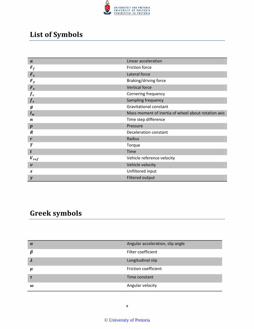
x

List of Symbols

𝒂 Linear acceleration 𝑭𝒇 Friction force 𝑭𝒙 Lateral force 𝑭𝒚 Braking/driving force 𝑭𝒛 Vertical force 𝒇𝒄 Cornering frequency 𝒇𝒔 Sampling frequency 𝒈 Gravitational constant 𝑰𝒘 Mass moment of inertia of wheel about rotation axis 𝒏 Time step difference 𝒑 Pressure 𝑹 Deceleration constant 𝒓 Radius 𝑻 Torque 𝒕 Time 𝑽𝒓𝒆𝒇 Vehicle reference velocity 𝒗 Vehicle velocity 𝒙 Unfiltered input 𝒚 Filtered output

Greek symbols

𝜶 Angular acceleration, slip angle

𝜷 Filter coefficient

𝝀 Longitudinal slip

𝝁 Friction coefficient

𝝉 Time constant

𝝎 Angular velocity


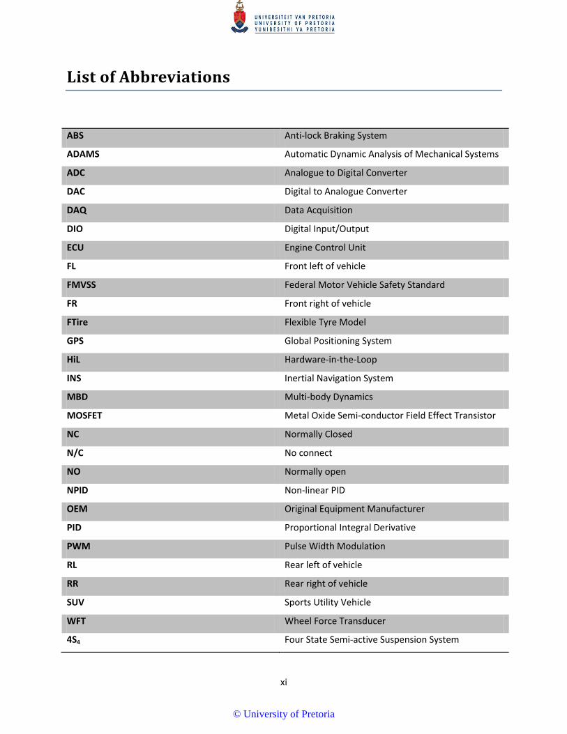
xi

List of Abbreviations

ABS Anti-lock Braking System

ADAMS Automatic Dynamic Analysis of Mechanical Systems

ADC Analogue to Digital Converter

DAC Digital to Analogue Converter

DAQ Data Acquisition

DIO Digital Input/Output

ECU Engine Control Unit

FL Front left of vehicle

FMVSS Federal Motor Vehicle Safety Standard

FR Front right of vehicle

FTire Flexible Tyre Model

GPS Global Positioning System

HiL Hardware-in-the-Loop

INS Inertial Navigation System

MBD Multi-body Dynamics

MOSFET Metal Oxide Semi-conductor Field Effect Transistor

NC Normally Closed

N/C No connect

NO Normally open

NPID Non-linear PID

OEM Original Equipment Manufacturer

PID Proportional Integral Derivative

PWM Pulse Width Modulation

RL Rear left of vehicle

RR Rear right of vehicle

SUV Sports Utility Vehicle

WFT Wheel Force Transducer

4S4 Four State Semi-active Suspension System


1

Chapter 1: Introduction and Literature

Introduction The safety of modern vehicles can be attributed to a wide range of complex systems that aim to prevent

loss of life, whether it assists the driver in an active sense or simply provides passive protection.

However, the effectiveness of the braking system of the vehicle has always been the primary factor that

will save occupant’s lives.

The World Health Organization (WHO) states that more than a million people die each year due to

motor vehicle accidents globally and is also the leading cause of death in young people aging between

15 – 29 (World Health Organization 2013). The American Journal of Public Health also found that motor

vehicle accidents are the leading cause of unintentional death, and is second overall for unnatural

deaths, preceded only by suicide (Rockett et al. 2012). Annual reports by South Africa’s leading road

safety initiative, Arrive Alive, describe the same trend and states a figure close to 14 000 fatalities for the

period of 1 April 2010 – 31 March 2011 (Road Traffic Management Corporation 2011). This document

further reports that faulty brakes is second on the list of contributing factors with a 15% contribution to

fatal vehicle accidents in the same period. Interestingly, poor road conditions were the largest

contributing environmental factor, responsible for 28% of fatal accidents.

With the increased popularity and proliferation of multi-purpose vehicles such as Sport Utility Vehicles

(SUVs), which is often used under off-road conditions, a new challenge appeared namely that ABS brake

performance is negatively affected by rough road conditions. Road input excitation from rough terrain

deteriorates braking performance which result in longer stopping distances due to a number of

suspension and tyre contributing factors. ABS on such terrains is faced with a particularly challenging

task as rapid pressure changes add further complications to the already noisy wheel speeds. Solving the

braking problem on rough terrains will provide increased safety to off-road drivers and motorists who

travel on roads with poor surface conditions.

1.1 The basics of braking The ability to bring a vehicle to rest is just as important as the driving force that is needed to propel it

forward. Braking safety is often incorrectly measured as the distance it takes for the vehicle to come to


2

a complete stop and should rather be a combination of the ability to steer the vehicle to avoid an

obstacle while braking in the shortest possible distance. As anyone who has participated in a skid-pan

driver training sessions will know, locking wheels during hard braking results in loss of directional

control. ABS provides the means to control brake pressure and hence wheel speed to prevent lock-up

and provides directional control of the vehicle to the driver. Many modern vehicles are equipped with

various active and intelligent systems that can stop the vehicle automatically without input from the

driver. However, all braking assist systems, regardless of their complexity, are subject to several

physical laws. The brake engineer exploits these laws and optimises the system to perform efficiently

within these laws.

1.2 Tyre force generation Tyres are often taken for granted by layman drivers, considering the fact that it is the sole component

responsible for transferring all external forces which may act on the vehicle, excluding aerodynamic

forces. Braking, acceleration and high speed cornering all generate large forces which act through four

palm-size contact patches between the road and the tyre. In the case with the pneumatic tyre, other

force generation mechanisms are present and therefore the dry friction laws are no longer applicable.

The rubber of the tyre exhibits both viscous and elastic properties that cause different force generating

mechanisms to occur. Gillespie (1999) explains the two primary mechanisms that generate tractive and

braking forces and are called adhesion and hysteresis. The adhesion mechanism is dominant and

generates its force from the intermolecular bonds between the rubber and the terrain. Adhesion

diminishes under wet conditions and when excessive slip is present. The hysteresis mechanism adds to

force generation in both directions due to the energy loss that occurs as the rubber deforms over the

terrain. Both of these mechanisms are involved in the generation of longitudinal and lateral forces and

are discussed in detail in the following sections.

1.2.1 Longitudinal force generation in tyres A tyre can generate tractive force due to relative movement between the stationary road and the

seemingly stationary rubber at the contact patch. This relative movement is called slip ratio and is

calculated as:

𝜆 =𝑣 − 𝜔𝑟𝑣

× 100% [1.1]


3

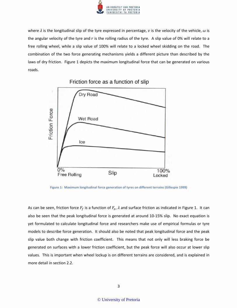
where 𝜆 is the longitudinal slip of the tyre expressed in percentage, 𝑣 is the velocity of the vehicle, 𝜔 is

the angular velocity of the tyre and 𝑟 is the rolling radius of the tyre. A slip value of 0% will relate to a

free rolling wheel, while a slip value of 100% will relate to a locked wheel skidding on the road. The

combination of the two force generating mechanisms yields a different picture than described by the

laws of dry friction. Figure 1 depicts the maximum longitudinal force that can be generated on various

roads.

Figure 1: Maximum longitudinal force generation of tyres on different terrains (Gillespie 1999)

As can be seen, friction force 𝐹𝑓 is a function of 𝐹𝑧, 𝜆 and surface friction as indicated in Figure 1. It can

also be seen that the peak longitudinal force is generated at around 10-15% slip. No exact equation is

yet formulated to calculate longitudinal force and researchers make use of empirical formulas or tyre

models to describe force generation. It should also be noted that peak longitudinal force and the peak

slip value both change with friction coefficient. This means that not only will less braking force be

generated on surfaces with a lower friction coefficient, but the peak force will also occur at lower slip

values. This is important when wheel lockup is on different terrains are considered, and is explained in

more detail in section 2.2.

Friction force as a function of slip


4

1.2.2 Lateral force generation in tyres The same two force generating mechanisms that is present with longitudinal force generation is also

present in lateral or steering force generation. Compliance in the tyre carcass causes a difference in

direction of tyre heading and direction of travel of the vehicle, and can be measured to be the slip angle,

𝛼. Just as the previous case, lateral force generation is dependant amongst others, 𝐹𝑧, 𝛼, and surface

friction. Once again, empirical formulas and tyre models are used to describe this force as no exact

equation exists to calculate it analytically.

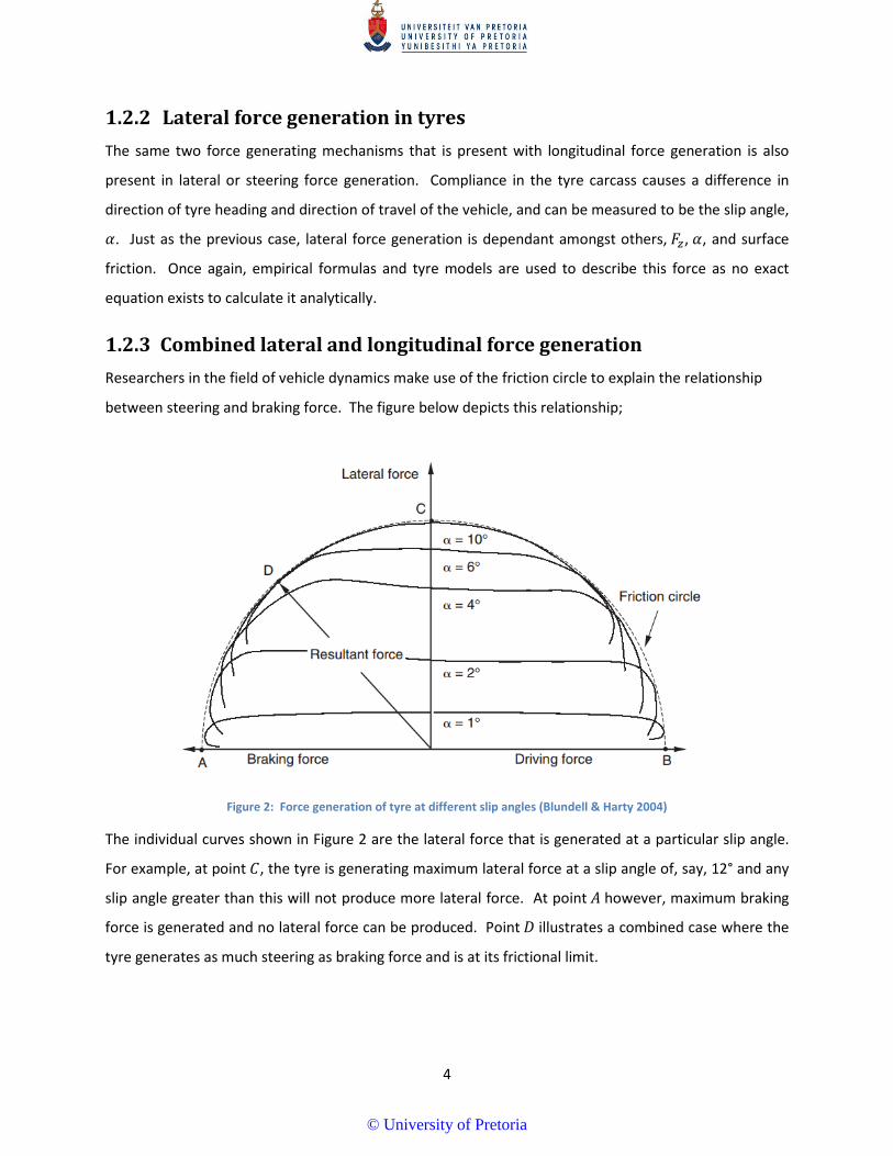
1.2.3 Combined lateral and longitudinal force generation Researchers in the field of vehicle dynamics make use of the friction circle to explain the relationship

between steering and braking force. The figure below depicts this relationship;

Figure 2: Force generation of tyre at different slip angles (Blundell & Harty 2004)

The individual curves shown in Figure 2 are the lateral force that is generated at a particular slip angle.

For example, at point 𝐶, the tyre is generating maximum lateral force at a slip angle of, say, 12° and any

slip angle greater than this will not produce more lateral force. At point 𝐴 however, maximum braking

force is generated and no lateral force can be produced. Point 𝐷 illustrates a combined case where the

tyre generates as much steering as braking force and is at its frictional limit.


5

1.3 The Anti-lock Braking System The inspiration for ABS research was sparked by one issue regarding pneumatic tyres: a locked tyre

cannot steer, as confined by the friction circle concept. Harned, Johnston, & Scharpf (1969) was the

pioneers of the ABS technology that allowed motor vehicle manufacturers to include anti-skid

technologies in production vehicles as early as 1970 under various trade names. The initial benefits of

ABS was soon realized and the United States Department Of Transport implemented the Federal Motor

Vehicle Safety Standard (FMVSS) 121 in the mid 1970’s which mandated ABS control for heavy trucks to

achieve prescribed stopping distances. These strict regulations were soon omitted from the standard,

due to the lack of reliable hardware at the time (Day & Roberts 2002). Fortunately most of these

hardware problems were solved during the 1980’s and the world has since arrived at a very reliable

system with the inclusion of on-board computers. It is now evident that the focus of ABS has since

migrated from simple hardware issues to the optimization of algorithms and software systems.

1.3.1 Anti-lock Braking System operation The goal of ABS is to control brake pressure in such a manner that the force generated by the tyre runs

along the dotted line between points 𝐴 and 𝐶 in Figure 2. This allows the driver to have a good

deceleration and lateral control of the vehicle regardless of pedal force input. Note that ABS may

increase stopping distance at the cost of providing lateral stability. Should the controller be optimally

designed to have maximum brake force at point C, the shortest stopping distance will be achieved but

no steering force will be generated.

Applied braking torque and thus braking force, in ABS systems is achieved by using an arrangement of

sensors and hydraulic valves to control brake pressure. Proximity sensors located at each wheel hub,

measure the passing of a serrated ring to determine wheel speed and if imminent wheel lock-up is

detected, the controller responds by reducing pressure to the concerned wheel.


6

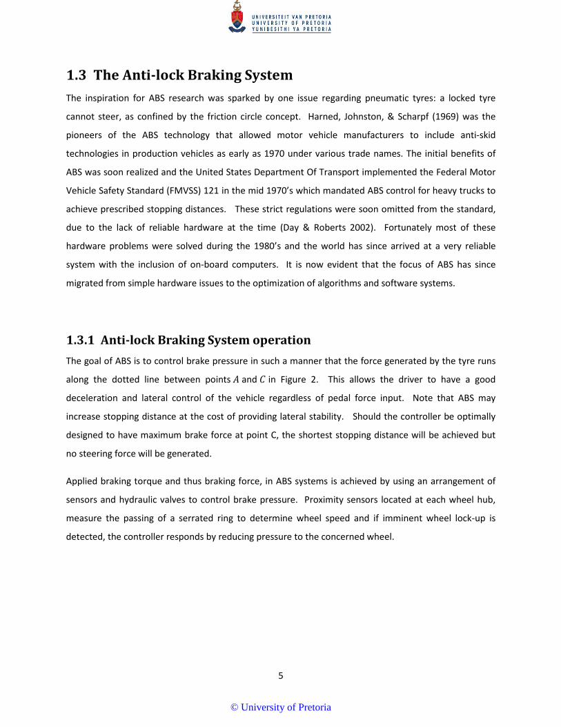
Figure 3: Simplified layout of ABS hardware

Here, 𝑣 is defined as the vehicle velocity, and 𝜔 is the angular velocity of the wheel. The controller

actuate hydraulic valves located in the modulator, as shown in Figure 3, in order to increase, reduce or

hold brake pressure. Hence the three states often used in literature, namely pump, dump and hold.

The modulator that is used in this study is a four channel Wabco model 478 407 022 0 (Wabco Vehicle

Control Systems 2003). Eight solenoid valves are housed inside that operate in pairs and are each of the

2/2 configuration, which means it can either block or allow flow. The shuttle valve is also an important

part of the modulator, and serves a double function, as acts as a pressure operated switch to sense

when the driver applies brake, and it isolates the master cylinder from the ABS hydraulic circuit when

the pump is activated to ensure that the pressure cannot escape back to the reservoir. This modulator

is also ideal for retro-fitting, as the unit contains its own pump, but not the control unit, as is often the

case.

The hydraulic modulator installed in the Land Rover Defender 110 test vehicle is the same model used in

the later “Puma” models that came standard with ABS, as is the case with the Original Equipment

Manufacturer (OEM) ABS vehicle used in section 6.3. The modulator houses eight solenoid valves, a

positive displacement pump and the shuttle valve. Fortunately the ECU is located separately from the

hydraulic unit and all control is made possible through a 15-pin plug. The 12V voltage supply switched

from the opto-coupler and relay pair is used to switch the solenoid valves.

Small accumulators, damping chambers and one-way valves are built into the modulator to aid with the

damping of pressure transients that develop when the valves are rapidly switched. Solenoid valves have

a certain response delay since the magnetic field has to develop. These delays are measured along with

the mechanical relay and pressure transient delays in the brake line using the pressure transducers


7

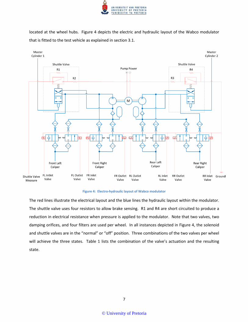
located at the wheel hubs. Figure 4 depicts the electric and hydraulic layout of the Wabco modulator

that is fitted to the test vehicle as explained in section 3.1.

Figure 4: Electro-hydraulic layout of Wabco modulator

The red lines illustrate the electrical layout and the blue lines the hydraulic layout within the modulator.

The shuttle valve uses four resistors to allow brake sensing. R1 and R4 are short circuited to produce a

reduction in electrical resistance when pressure is applied to the modulator. Note that two valves, two

damping orifices, and four filters are used per wheel. In all instances depicted in Figure 4, the solenoid

and shuttle valves are in the “normal” or “off” position. Three combinations of the two valves per wheel

will achieve the three states. Table 1 lists the combination of the valve’s actuation and the resulting

state.


8

Table 1: Valve combinations and resulting state

Inlet Valve Outlet Valve State

Off Off Pump

On On Dump

On Off Hold

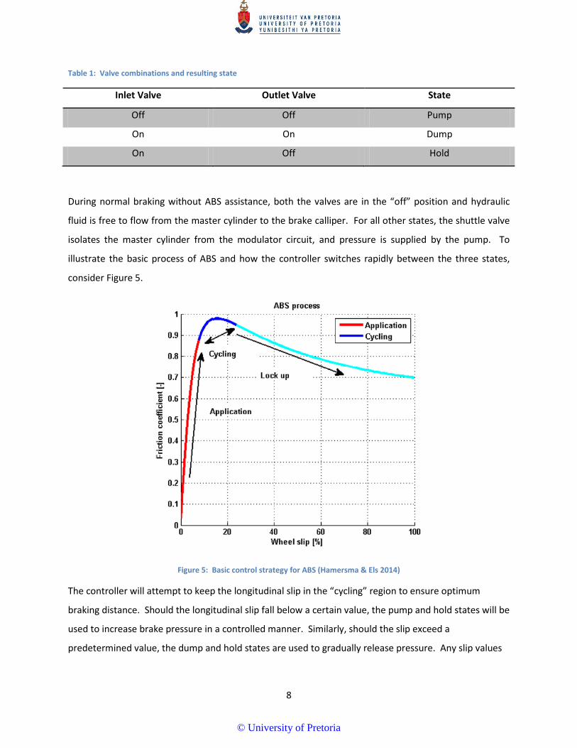
During normal braking without ABS assistance, both the valves are in the “off” position and hydraulic

fluid is free to flow from the master cylinder to the brake calliper. For all other states, the shuttle valve

isolates the master cylinder from the modulator circuit, and pressure is supplied by the pump. To

illustrate the basic process of ABS and how the controller switches rapidly between the three states,

consider Figure 5.

Figure 5: Basic control strategy for ABS (Hamersma & Els 2014)

The controller will attempt to keep the longitudinal slip in the “cycling” region to ensure optimum

braking distance. Should the longitudinal slip fall below a certain value, the pump and hold states will be

used to increase brake pressure in a controlled manner. Similarly, should the slip exceed a

predetermined value, the dump and hold states are used to gradually release pressure. Any slip values


9

less than the slip value at the peak friction coefficient can be utilised as valuable lateral control to steer

the vehicle while braking.

Blundell & Harty (2004) states that the effectiveness of any ABS strategy is mainly dependent on the

estimation of the friction coefficient of the road and the sophistication of the vehicle velocity

calculation. Aly, et al. (2011) labels the ABS control problem as a highly non-linear one, because of the

complex relationship between friction and slip. It is thus evident that the optimal ABS controller is one

that is only concerned with the friction coefficient and will base the control of brake pressure around

this value. Several control strategies have been employed in the past and the authors list the more

common strategies. A summary of the more relevant methods are given below.

I. Bang-bang control

The control method used in this study is bang-bang control. It is also the earliest and simplest strategy

used on motor vehicles for brake pressure control. Angular acceleration and longitudinal slip of the

wheel are controlled by using the three control states, pump, dump and hold. Several phases are

defined through which the controller regulates brake pressures, either by abruptly increasing or

decreasing pressure. The pump and dump states are also used in an alternating fashion with the hold

state to achieve gradual pressure release or build-up. In essence, this control strategy uses a peak

seeking approach to find the maximum longitudinal force and in the process of doing so, leaves room for

lateral force generation when the peak is not attained. Bauer & Bosch (1999) describes the basic

algorithm and Day & Roberts, (2002) implemented it in the Human Vehicle Environment MBD software

package. Kempf et al. (1987) explains a real time simulation implementation of this algorithm. The use

of this algorithm is explained in more detail in section 1.3.2, and Chapter 2.

II. Classical PID and NPID control

Proportional Integral Derivative control is an old and widely used method to control almost any

machine. Direct PID control is difficult to implement practically in ABS as the brake pressure cannot be

controlled in an analogue fashion, although newer hydraulic modulators can incorporate pulse width

modulated (PWM) solenoid valves to facilitate pseudo analogue control. This control method finds its

place in the simulation environment as it provides a fast and easy solution to a somewhat realistic ABS

model. Bhivate (2011) derives the equations of motion for a quarter-car model and use ideal, parallel

and series PID-type approaches to control longitudinal slip.


10

III. Adaptive control based on gain scheduling

The change in environmental parameters can have a severe effect on the performance of ABS, if the

control strategy assumes these values to be constant. Thus, several approaches incorporate adaptive or

intelligent methods for estimating these parameters or changing the normal control cycle to better suit

the different environment conditions that can be encountered. The simplest way to achieve this is to

have a family of linear controllers and a single variable that dictates which linear controller to use during

which scenario. Liu & Sun (1995) explains that friction coefficient, and thus optimal slip, is dependent

on vehicle speed and uses this variable to decide which gains to use in the control of the braking torque.

IV. Intelligent fuzzy logic control

Fuzzy logic has been used in the control of ABS in recent years as a novel solution to the unknown

environmental parameters. Classic fuzzy logic yields a large amount of fuzzy rules that complicates the

construction and influences the performance of the controller so it is often based on sliding-mode

control. This approach has fewer fuzzy rules and provides more robustness against environmental

parameters. Ozdalyan (2008) describes such a strategy that controls slip by prescribing the rate of

pressure change which is numerically integrated to produce brake pressure output.

Current state-of-the-art ABS research is mainly focussed on electrically driven wheels, as it is believed

that these vehicles will become more popular in the near future. Since electronic torque control on a DC

motor is simpler and more accurate than hydraulic bang-bang control, better ABS systems can be

developed on electrically driven vehicles. Ivanov et al. (2014) presents promising straight line braking

results superior to hydraulic ABS by using Hardware-in-the-Loop (HiL) simulation.

1.3.2 Bosch ABS algorithm The Bosch algorithm, as it is most commonly known as, was introduced in commercial vehicles in 1978,

when the use of digital electronics were introduced into the automotive industry (SAE Standard, 1992).

The bang-bang control strategy that this algorithm follows is somewhat crude when compared to newer

control methods, as it follows simple “if-else” logic. Although it proves more challenging to simulate

compared to the other methods above, it is by far the simplest to implement in a physical system, since

it requires simple hydraulic hardware such as solenoid valves and positive displacement pumps.

The only input required for the classic Bosch algorithm are the four wheel speed sensors. From this,

vehicle velocity is estimated, longitudinal slip is calculated and angular acceleration is derived from the


11

angular velocity inputs. All decision making and pressure control follows from these calculated values.

Augmenting the system with extra sensors such an accelerometer or a Global Positioning System (GPS)

will improve velocity estimation or eliminate the need for estimation completely, but the system cannot

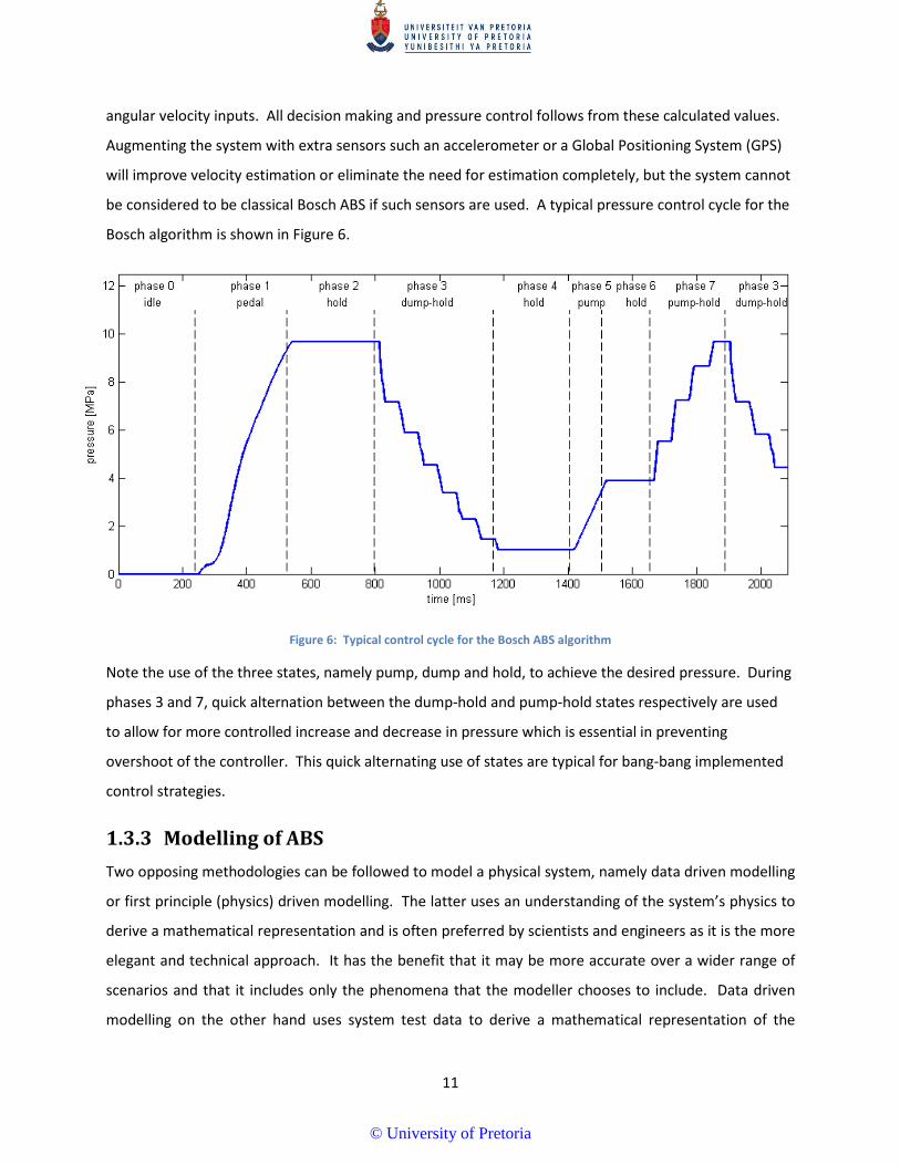
be considered to be classical Bosch ABS if such sensors are used. A typical pressure control cycle for the

Bosch algorithm is shown in Figure 6.

Figure 6: Typical control cycle for the Bosch ABS algorithm

Note the use of the three states, namely pump, dump and hold, to achieve the desired pressure. During

phases 3 and 7, quick alternation between the dump-hold and pump-hold states respectively are used

to allow for more controlled increase and decrease in pressure which is essential in preventing

overshoot of the controller. This quick alternating use of states are typical for bang-bang implemented

control strategies.

1.3.3 Modelling of ABS Two opposing methodologies can be followed to model a physical system, namely data driven modelling

or first principle (physics) driven modelling. The latter uses an understanding of the system’s physics to

derive a mathematical representation and is often preferred by scientists and engineers as it is the more

elegant and technical approach. It has the benefit that it may be more accurate over a wider range of

scenarios and that it includes only the phenomena that the modeller chooses to include. Data driven

modelling on the other hand uses system test data to derive a mathematical representation of the


12

system and may prove easier for more complex systems and can be more accurate for a specific

scenario.

Ozdalyan & Blundell (1998) explain a detailed anti-lock brake model of a single wheel in MSC Automatic

Dynamic Analysis of Mechanical Systems (ADAMS). Pressure and control logic was defined in ADAMS

and the model required no additional software to perform the simulation. Although this model was only

a quarter car model, longitudinal load transfer and other non-linearities such as rubber suspension

bushes and bump stops were also included. The model did not calculate its velocity by using wheel

speed, but instead used vehicle velocity from ADAMS to calculate slip and perform its control.

Measuring vehicle velocity in this way is not a good representation of the reality and should be used

with caution during modelling of ABS.

A more advanced simulation model was used by Wang, Song, & Jin (2010) to incorporate a co-simulation

model between AMESim and Simulink/Stateflow. The control logic was modelled with the Stateflow

toolbox which greatly simplifies model complexity if a finite number of control states are present.

AMESim features a hydraulic library which the authors use to model the solenoid valves and positive

displacement pump in the modulator. The controller passes discrete on/off command signals to the

hydraulic subsystem to switch valves and pumps to control brake pressure. No validation was done to

correlate simulation results and test data.

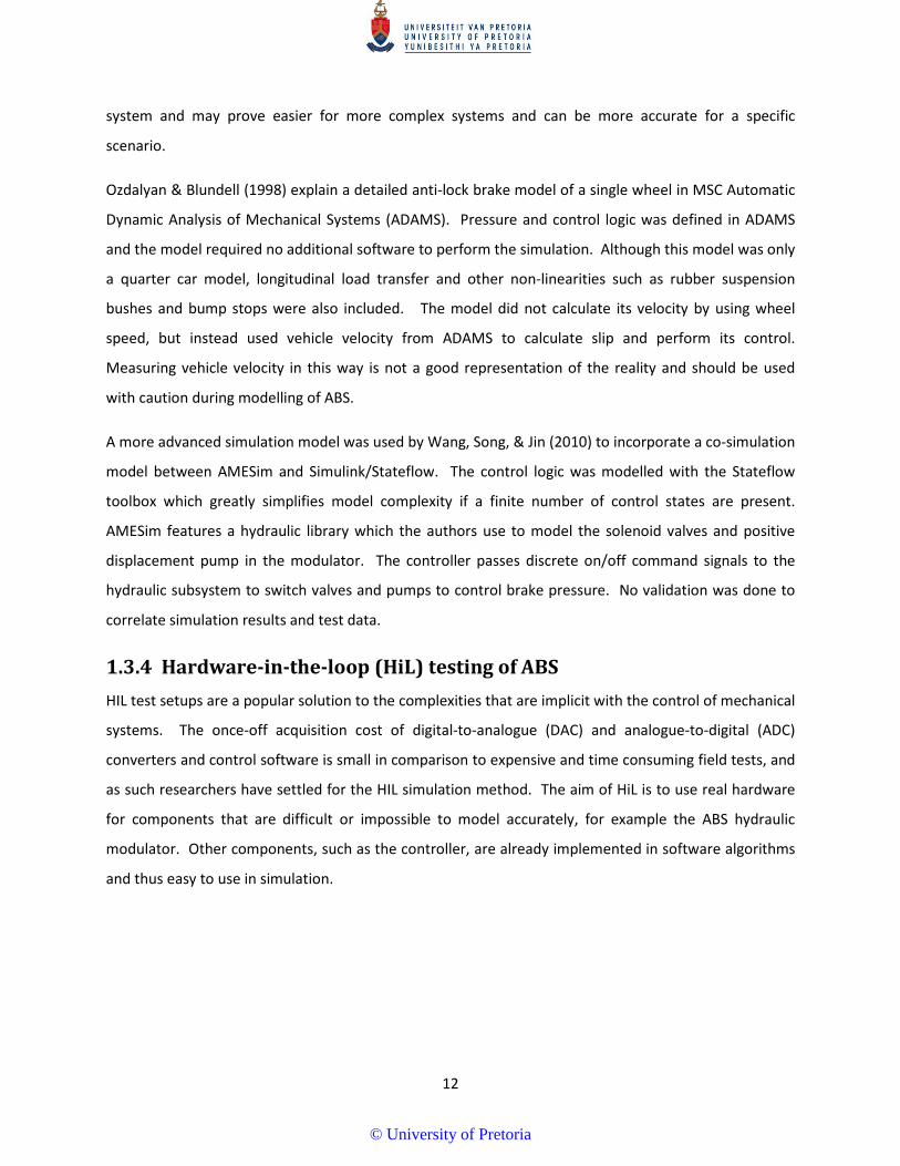
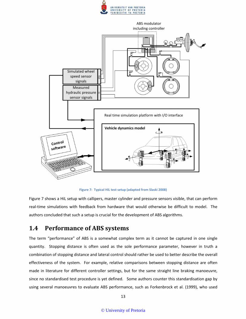
1.3.4 Hardware-in-the-loop (HiL) testing of ABS HIL test setups are a popular solution to the complexities that are implicit with the control of mechanical

systems. The once-off acquisition cost of digital-to-analogue (DAC) and analogue-to-digital (ADC)

converters and control software is small in comparison to expensive and time consuming field tests, and

as such researchers have settled for the HIL simulation method. The aim of HiL is to use real hardware

for components that are difficult or impossible to model accurately, for example the ABS hydraulic

modulator. Other components, such as the controller, are already implemented in software algorithms

and thus easy to use in simulation.


13

Figure 7: Typical HiL test setup (adapted from Slaski 2008)

Figure 7 shows a HiL setup with callipers, master cylinder and pressure sensors visible, that can perform

real-time simulations with feedback from hardware that would otherwise be difficult to model. The

authors concluded that such a setup is crucial for the development of ABS algorithms.

1.4 Performance of ABS systems The term “performance” of ABS is a somewhat complex term as it cannot be captured in one single

quantity. Stopping distance is often used as the sole performance parameter, however in truth a

combination of stopping distance and lateral control should rather be used to better describe the overall

effectiveness of the system. For example, relative comparisons between stopping distance are often

made in literature for different controller settings, but for the same straight line braking manoeuvre,

since no standardised test procedure is yet defined. Some authors counter this standardisation gap by

using several manoeuvres to evaluate ABS performance, such as Forkenbrock et al. (1999), who used

Simulated wheel speed sensor

signals Measured

hydraulic pressure sensor signals

Real time simulation platform with I/O interface

In O

ut

ABS modulator including controller

Vehicle dynamics model


14

straight line braking manoeuvres to J-turns and lane changes between nine vehicles to determine the

best performing ABS equipped vehicle. Although this approach proves which test vehicle has the best

ABS system in the sample size, it provides no insight as to how close to optimal the controller performs

or how it compares to a benchmark. Arrigoni et al. (2015) uses a novel approach worth mentioning,

where a band of slip values are shown in which the largest portion of the normalised braking force is

accumulated on the longitudinal force-slip plot. A narrow band about the peak represents little

deviation from the peak longitudinal force point and will ensure good stopping distance but little lateral

control. Contrary to this, a band across a wide range of slip values shows that the controller allows for a

wide range of slip and will ensure better lateral control.

1.4.1 Terrain effects The study of terramechanics is concerned with the interaction between tyre and terrain and is a

research field that is not yet fully understood. Taylor & Sokolovskij (2010) found that deformable terrain

such as snowy or sandy roads provide better stopping distances in the case of non-ABS brakes because

of the wedging effect that occurs when loose material piles in front of the locked tyre. While it provides

good longitudinal force generation, little sacrifice to steering force is made and a locked tyre can steer

adequately. Deformable terrain is a complex science and is not included in the scope of this study.

With the remaining case of undeformable or simply hard terrains, the effects of surface roughness are

considered. Flat terrain is usually the choice of input condition to ABS researchers, because it is easy to

simulate and optimise for different friction coefficients. Research has found that, for most hard terrains

with a good fiction coefficient, ABS equipped vehicles will achieve shorter braking distances than

vehicles without ABS assistance since the tyre can operate closer to its peak force generation point

(Forkenbrock et al. 1999), (Eriksson 2014).

In the case of rough terrains, several other effects are present that interfere with the normal ABS

operation and lead to poor stopping distances. Road input excitation leads to, amongst others, normal

load variations due to axle oscillations and results in deteriorated ABS performance. This becomes

especially clear at the resonance region of the suspension system (Van der Jagt et al. 1989). Vehicle

body motions such as roll, pitch and yaw that are excited by rough road input also disturb the slip

control of the wheel (Reul & Winner 2009). Sudden changes in wheel speed, as the wheel encounters

an obstacle for example, will also result in fluctuations in adhesion, since peak friction of the tyre is

dependent on wheel speed (Satoh & Shiraishi 1983). Several other issues are also listed by Koylu &


15

Cinar (2011) with specific focus on the effect of worn dampers on ABS. Controller malfunction can occur

because of noisy wheel speed sensors (Blundell & Harty 2004), and faults in the algorithm that leads to

poor control desicions (Watanabe & Noguchi 1990).

1.4.2 Suspension effects Damper manufacturers have always exploited the claim that worn dampers lead to poor stopping

distances and loss of steering. This is true for the most part and is supported by Koylu & Cinar (2011)

that found that higher damping usually benefits braking performance, and Reul & Winner (2009) that

concluded that shorter braking distances are obtained by less slip oscillations. In essence Reul & Winner

(2009) argue that the mean friction coefficient, will approach the maximum value, as slip oscillations are

minimised. Put in a mathematical relation, the objective:

𝜇𝑚𝑒𝑎𝑛 → 𝜇𝑚𝑎𝑥 [1.2]

can be achieved by minimising slip variation, expressed as:

𝜆𝑜𝑝𝑡𝑖𝑚𝑢𝑚 − 𝜆𝑏 → 0 [1.3]

by minimising vertical load variations. In the above equations, 𝜇𝑚𝑒𝑎𝑛 and 𝜇𝑚𝑎𝑥 are mean and maximum

friction coefficients respectively, and 𝜆𝑜𝑝𝑡𝑖𝑛𝑢𝑚 and 𝜆𝑏 are the peak and brake longitudinal slip

respectively. The vertical load variations are controlled by the dampers and thus play a vital role in the

performance of rough terrain braking. The authors proposed an intelligent control stategy that uses a

combination between an semi-active suspension system and the ABS controller to optimise braking

performance. The authors defined a single equation that relates wheel load and braking torque to

change in wheel angular velocity;

Δ𝜔 = ��𝜇 𝜆𝑏(𝑡)𝐹𝑧(𝑡) 𝑟 𝑑𝑡 − �𝑇(𝑡) 𝑑𝑡�1𝐼𝑤

[1.4]

where 𝐹𝑧 is the vertical load of the wheel, 𝑟 is the rolling radius, 𝑇 is the braking torque and 𝐼𝑤 is the

rotational inertia of the wheel. Equation {1.8} shows that variations in the wheel’s angular velocity

result from the time domain integral of the vertical wheel load and brake torque. The controller

switches the damper setting on the suspension system and adjusts the brake force operation point of

the ABS, depending on the current state of the semi-active damper and on the value of the dynamic


16

wheel load integral. The second integral is the braking torque integral and ABS will naturally vary this

value. Test results of this combined brake and suspension controller showed improved ABS braking

performance on rough terrain vs standard ABS braking on the same terrain.

Hamersma & Els (2014) determined that the spring and damper characteristics play an important role in

ABS braking on rough roads and can influence stopping distances significantly. The authors used a

Monte-Carlo simulation approach and found that lower stiffness for the rear suspension produced the

best results while lower stiffness at the front suspension yielded the worst results. Moderate to high

damping for the front suspension also proved advantageous. It was also found that the suspension

settings for optimal braking performance are vehicle velocity dependent.

1.4.3 Tyre effects Another major contributor to ABS performance is the tyres. The contribution of the tyre to the rough

road braking problem can be severe and has to be understood. Literature lists a number of tyre effects

that influence the control of brake pressure to achieve best braking performance. According to Zegelaar

(1998), the in-plane rotational and longitudinal wheel hop vibration modes are of the most concern to

rough terrain braking as it affects the measurement of slip the most. These modes form part of the so-

called rigid ring modes that often occur as the first and second mode shapes of the tyre. Becker & Els

(2011) explain a method of determining the mode shapes and it was determined that the in-plane

rotational mode occur at 31.1Hz while the longitudinal wheel hop mode is at 18.4Hz for the tyre used in

this study at a pressure of 200kPa preloaded with a quarter of the vehicle mass. Adcox et al. (2013)

found that the torsional dynamics of the tyre can influence ABS performance by supplying false

information to the controller that affects control. The authors found that a wheel speed filter with a cut-

off frequency lower than the torsional natural frequency of the tyre effectively eliminates this problem.


17

1.5 Tyre models As for most vehicle dynamic simulations, tyres contribute extensively to the complexity of the problem.

This is due to the highly non-linear visco-elastic road contact mechanism, which leads to challenging

mathematical modelling. Furthermore, rough terrain simulation adds various other complexities such as

vibrational excitation of the carcass and complicated contact patch mechanics to the problem. Thus, the

choice of tyre model will ultimately determine the success of any ABS simulation. A high fidelity tyre

model with good transient capabilities and accurate contact patch dynamics, which is valid up to high

frequencies, is needed. The tyre model must be capable of describing lateral, longitudinal and vertical

tyre forces accurately.

High fidelity models are available today but require extensive computational power. Therefore, a

careful compromise should be found for a successful simulation. In general, tyre models can be

classified into three categories, namely physics based, semi-empirical and data-based models. Physics

based tyre models uses a complex set of mathematical equations to describe the force generation and

surface interaction of the tyre. Research has shown that these models can accurately predict forces

over uneven terrain, but requires significantly more computational effort to solve. In contrast to physics

based models, data-based models simply use look-up tables and interpolation methods to return force

values. Semi-empirical models find its place somewhere between the above mentioned models and are

often formulated on an ad-hoc basis.

1.5.1 Pacejka ’89 and ’94 models: The Pacejka tyre models, often referred to as Magic Formula tyre models, use curve fits generated from

experimental test data that describe tyre forces for given inputs. The sideslip angle, longitudinal slip,

camber angle and the normal force is required to obtain lateral force, longitudinal force and the self-

aligning moment. Due to its simplistic lookup type of formulation, it is mainly used for handling

simulations on smooth roads. Initially a single point contact model with linear stiffness and damping

was used to calculate the vertical force, but various other contact models are available today, such as

the 3D enveloping and equivalent volume models that might prove useful for rough road simulation.

Stallmann (2013) found that reasonable correlation could be obtained with the 3D enveloping contact

model over discrete obstacles such as a cleat, but that none of the contact models give acceptable

results when rough tracks are concerned.


18

1.5.2 Fiala model: The Fiala tyre model uses less input parameters than the Pacejka89 and 94 models to describe the same

output forces. It is different from the Pacejka models in the sense that it requires stiffness and damping

parameters, as well as some tyre geometry. This model is considered to be simple a model that requires

few inputs and produce less accurate results (Oosten 2011). This tyre is used by some researchers in

ABS simulations such as Ozdalyan & Blundell (1998), but are restricted to smooth flat roads. The Fiala

tyre model is too simple, too inaccurate and does not simulate modal responses. Thus, this model is not

a suitable tyre model for simulating ABS over rough terrain.

1.5.3 Pacejka 2002 model: The Pacejka 2002 model is an advancement of the basic Magic Formula approach in the sense that the

several non-linear characteristics and a rigid ring option are added as additional features. The basic

model can make use of an “advanced transient mode” that make the model valid up to 15 Hz, and if

used with the available “belt dynamics”, the validity of the model holds to 70 – 80 Hz (MSC Software

2013). This model also supports the 3D enveloping contact model, which is recommended by MSC for

rough roads. Contact models will be explained in more detail in section 1.6.

The Pacejka2002 model was modified by Jaiswal, et. al. (2010) to incorporate a first order differential

equation to account for the important relaxation length phenomenon. Jaiswal et al. (2010) developed

special tyre models for ABS simulation which includes a stretched string, modified stretched string and

contact mass models. These models are all based on the Pacejka 2002 tyre model, but provide better

transient modelling by describing the relaxation length with first order differential equations that are

dependent on vertical load and slip angle. The authors successfully demonstrate the importance of the

relaxation length in the simulation of ABS.

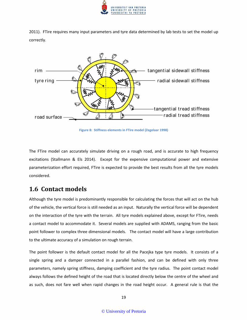
1.5.4 FTire model: The Flexible Ring Tire (FTire) model, as the name suggests, is an advanced tyre model that uses a flexible

ring connected to a rigid hub, shown in Figure 8. Gipser (1999) developed the model over the past 15

years. The tyre model is based on a structural dynamics approach unlike the empirical or semi-empirical

models explained before. Radial, tangential and lateral stiffness’s define a flexible ring and are made up

of some 100 to 200 “belt elements” that are used to numerically approximate the generated tyre forces

(Stallmann 2013). This model takes modal responses into account and is accurate up to 120 Hz (Oosten


19

2011). FTire requires many input parameters and tyre data determined by lab tests to set the model up

correctly.

Figure 8: Stiffness elements in FTire model (Zegelaar 1998)

The FTire model can accurately simulate driving on a rough road, and is accurate to high frequency

excitations (Stallmann & Els 2014). Except for the expensive computational power and extensive

parameterization effort required, FTire is expected to provide the best results from all the tyre models

considered.

1.6 Contact models Although the tyre model is predominantly responsible for calculating the forces that will act on the hub

of the vehicle, the vertical force is still needed as an input. Naturally the vertical force will be dependent

on the interaction of the tyre with the terrain. All tyre models explained above, except for FTire, needs

a contact model to accommodate it. Several models are supplied with ADAMS, ranging from the basic

point follower to complex three dimensional models. The contact model will have a large contribution

to the ultimate accuracy of a simulation on rough terrain.

The point follower is the default contact model for all the Pacejka type tyre models. It consists of a

single spring and a damper connected in a parallel fashion, and can be defined with only three

parameters, namely spring stiffness, damping coefficient and the tyre radius. The point contact model

always follows the defined height of the road that is located directly below the centre of the wheel and

as such, does not fare well when rapid changes in the road height occur. A general rule is that the


20

model is accurate for obstacles that have wavelengths longer than the tyre radius, and will thus not

accurately describe the forces for the rough terrain scope of this study.

The 3D enveloping contact model is a more realistic approach than the point follower model. A

predetermined number of egg-shaped cams are implemented such that they represent the edge of the

contact patch. This contact model effectively filters the road input for short wavelength obstacles by

lengthening the input response and reducing its magnitude. Eleven parameters defined by the user are

used to calculate the size of the contact patch, which in turn calculates the effective tyre deflection.

Once again a spring stiffness and a damping constant are defined and the normal force calculated. The

3D enveloping contact model is also recommended by MSC Software as the contact model of choice

when obstacles with wavelengths shorter than tyre circumference are present in the simulation.

A more advanced contact model is the equivalent volume contact. This model approximates the tyre as

a set of cylinders spaced across the width and the solver can accurately calculate the intersection

volume between the road and the unloaded tyre, from which friction and normal force amongst others

can then be calculated. This type of contact model is considered to be more accurate on rough roads

and can accurately calculate tyre forces on abrupt changes in road geometry. It was also found that this

model is suitable for larger tyres (Stallmann, 2013). The above discussed contact models are shown in

Figure 9.

Figure 9: Point follower, 3D enveloping and equivalent volume contact models (Stallmann 2013)


21

1.7 Recommended tyre models Antoine et al.(2005) suggests the uses of a tyre model for the simulation of ABS that can accurately

predict dynamic tyre responses up to 100Hz. This statement excludes the Pacejka89 and 92 models but

suggests that both the Pacejka 2002 model with belt dynamics as well as FTire should provide adequate

results. MSC Software, which is the developers of the multi-body dynamic software package ADAMS,

recommends the choice of tyre models for ABS or rough terrain simulation as indicated in Table 2.

Table 2: Recommended tyre models for use in ADAMS (MSC Software web page 2013).

Event/Maneuver PAC89 PAC94 PAC2002 PAC2002* Fiala FTire

ABS braking distance o/+ o/+ + + o +

Braking/power-off in a turn o o + + o o/+

Cornering on uneven roads o o o/+ + o +

Braking on uneven roads o o o/+ + o +

Driving over uneven road - - - + - +

ABS braking control o o o/+ + o +

Chassis control systems >8 Hz - - o/+ + - +

* PAC2002 with belt dynamics

-

o

o/+

+

It can be seen from Table 2 that the Pacejka 2002 and FTire models are the only two tyre models that

have the potential to provide the best simulation results for this study. Fortunately the University of

Pretoria has a validated FTire model of the Michelin LTX 235/85 R16 tyre that will be used in this study.

Furthermore, the University has also developed a capable test vehicle that will be used to complete the

experimental portion of this study. Since the vehicle is a 1997 Land Rover Defender 110 TDi, it is not

fitted with ABS, however the semi-active suspension system together with the various permanent

mounted sensors makes this vehicle an attractive choice for ABS research. Several research outputs in

previous years have also created a large database of test data and simulation models that can be

Not possible / Not realistic

Possible

Better

Best to use


22

adapted to fit this specific study, rather than having to model a vehicle from the beginning. Sport Utility

Vehicles, such as this Land Rover model, also provides a relatively unexplored research opportunity, as

these vehicles are often expected to perform impossible tasks on rough terrain.

1.8 Scope of this study Although ABS systems have seen a long development history and has been implemented almost

universally on passenger vehicles, several areas for improvement still exists.

ABS performance on rough terrain deteriorates significantly due to several contributing factors which

can all be attributed to road excitation. As a possible solution to the problem, it was found that some

alterations to the ABS algorithm have to be made. Furthermore, the use of semi-active suspension can

also be used to counter these negative effects. In order to analyse and improve ABS algorithms, a

vehicle simulation model that can accurately simulate braking on rough terrain is required. This model

needs to be verified against experimental results before it can be used with confidence. Experimental

validation will require a test platform, fitted with ABS brakes, where full access to the controller and

control algorithm is essential.

The choice of a suitable tyre model is of extreme importance for any vehicle simulation. Different tyre

models were compared in order to find a suitable choice to use in the simulation of ABS. The opinions

from previous research and the recommendations from the software developers all point to FTire as the

best suited tyre model for rough road ABS simulation.

This study will aim to implement a functional Anti-lock Braking System in a test vehicle by using the

Bosch algorithm. The test vehicle shall make use of wheel speed sensors alone, as is the case with

conventional ABS. A simulation model will also be developed that can be used to determine the factors

contributing to the deterioration of ABS performance on rough terrain. Tests shall be performed mainly

on surfaces with higher friction coefficients but also high roughness and validated against the simulation

model to ultimately provide efficient means to develop countermeasures to the rough terrain braking

problem.

Chapter 2 covers the detail of the Bosch ABS algorithm, including how the thresholds which the system

are designed to function within were chosen and how the reference velocity, longitudinal slip and

angular acceleration is calculated on the on-board computer. A brief discussion on intelligent algorithms

concludes the chapter.


23

The test vehicle, including all the sensors and systems used in this study, is discussed in Chapter 3. The

hydraulic and electrical system layout is clearly illustrated. The use of a Wheel Force Transducer (WFT)

is also covered in detail. The multibody dynamics simulation model, together with all the relevant

details around the suspension system and tyre model is included here. Simulink was used extensively,

and the layout behind the subsystems, such as the driver model and the pressure look-up is also

explained.

Chapter 4 deals with how the tables are constructed that are used in the pressure look-up subsystem.

This forms the heart of the simulation portion of this study and a list of assumptions is given at the

beginning of this chapter. Naturally the electro-hydraulic system will introduce some response delays

into the system which are measured and modelled into the Matlab/Simulink model.

The validation of the simulation model is done in Chapter 5. The pressure lookup forms the basis of the

entire simulation model and is validated first. The reference velocity plays an important role in the

calculation of longitudinal slip and is first validated over rough terrain with ABS deactivated. Thereafter,

simulation results and test data for different terrains are plotted on the same figures to validate the

multi-body dynamics model, first for flat terrain and then for the Belgian paving.

Chapter 6 depicts the deterioration of ABS performance on rough terrains by using the same results as

before, but comparing the results and test data separately for different terrains. Thereafter, conclusions

can be drawn as the deterioration of ABS performance can clearly be seen between the various terrains.

The last chapter lists conclusions that were found during the interpretation of the results in Chapter 6.

A list of recommendations are also given, should any attempt be made in future to improve this study.


24

Chapter 2: Control Algorithm

Introduction This study uses the Bosch ABS algorithm, as published by Bauer & Bosch (1999), as baseline. This bang-

bang control approach switches solenoid valves in the hydraulic modulator to control brake pressure

and thus longitudinal slip and angular acceleration to prevent wheel lock-up.

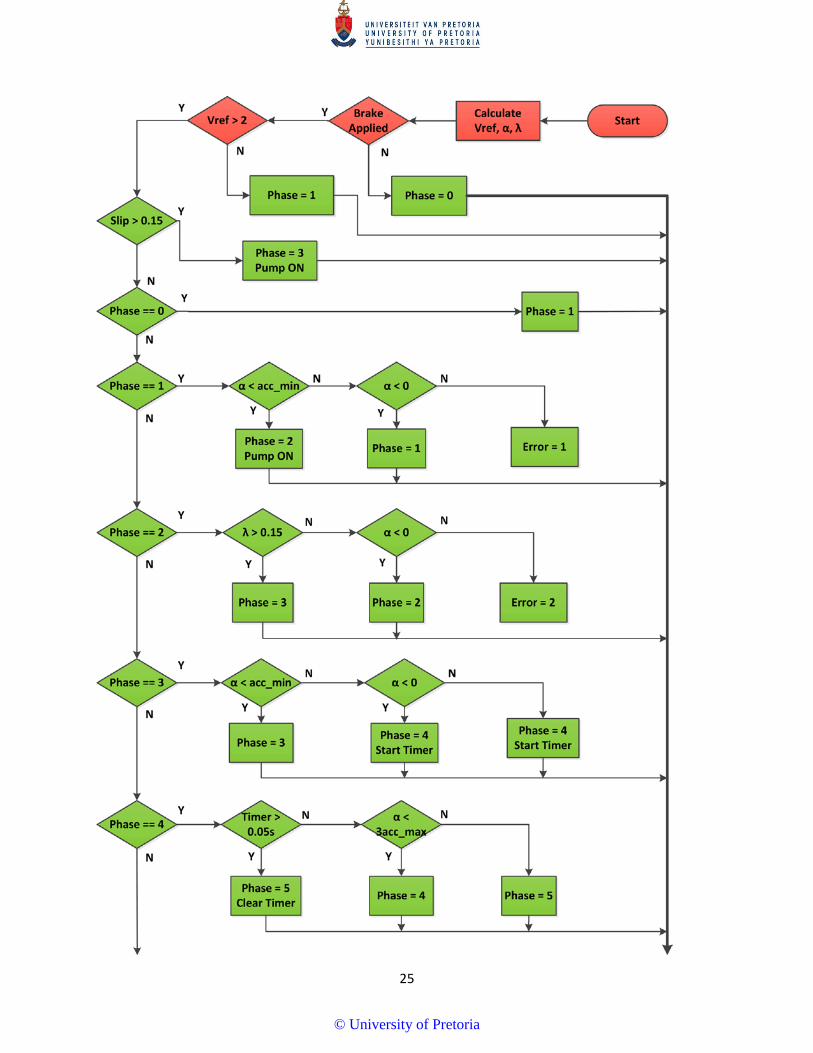
2.1 Bosch algorithm The Bosch algorithm is represented in the flow chart indicated in Figure 10 to clearly show the decision

making logic. It is later implemented in C-code in section 3.1.4 and in Matlab in section 3.2.3. The

calculation of the reference velocity poses its own complexities and will be explained separately. The

Bosch algorithm has three important parameters that dictate its performance, namely the maximum

and minimum angular acceleration thresholds, and the maximum allowable slip. These parameters

were tuned during simulation and the starting point was taken as reported by Day & Roberts (2002).

Naturally, the algorithm cannot perform equally well on all road conditions, thus the slip threshold and

deceleration constant can be adaptive, as explained later in section 2.7. However since the scope of this

study is limited to high friction surfaces and the adaptive capability will be disregarded.

The flow chart in Figure 10 depicts the control logic for the ABS system. The control cycle starts in the

top right corner of the figure. The reference velocity, rotational acceleration and longitudinal slip are

calculated for each wheel. Several logical checks are then performed to ensure that the controller only

acts when necessary. For example, the brakes must be actuated by the driver for ABS to be active.

Numerical instability may also occur at low speeds with the calculation of slip and the controller is

programmed such that it should become inactive at vehicle speeds less than 2 m/s.


25


26

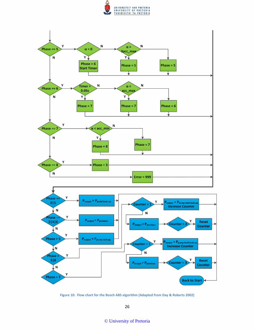
Figure 10: Flow chart for the Bosch ABS algorithm (Adapted from Day & Roberts 2002)


27

The flow chart in Figure 10 is divided into three groups, each with its own colour assigned. Red indicates

the calculation of the inputs that the controller requires, whereas green indicates the control logic

portion of the system, and blue signifies the part of the algorithm where the hydraulic modulator is

controlled. After completing the initial checks, nine phases are defined that mark a specific state of ABS

based on logic statements. Once the correct phase of operation has been selected, the modulator is

actuated to dictate pressure control. All the phases are explained in detail below:

Phase 0: The brake pedal is not actuated and no power is supplied to the valves and pump. The

controller will spend most of its time in this phase during acceleration and cruising. Reference velocity,

angular acceleration and longitudinal slip are calculated but the controller remains dormant. This is also

the phase at which traction control can be implemented.

Phase 1: Initial pedal application. When the driver applies enough force to the brake pedal to actuate

the shuttle valve, the controller measures the change in resistance and monitors angular acceleration

and slip. No power is delivered to the valves or pump yet and brake fluid is free to flow between the

master cylinder and the brake callipers such as during normal braking. If the angular acceleration of the

wheel does not become negative, an error code 1 is registered and indicates that hydraulic fluid is low

or that air is present in the concerned hydraulic line.

Phase 2: Hold or pressure maintaining phase. The minimum angular acceleration threshold of a wheel

has been exceeded and the controller is now activated. Power is supplied to the pump and the

concerned valves are set to the hold position to maintain the current pressure to the calliper. The

controller shall remain in this phase until the slip threshold is exceeded. The slip value at the start of

this phase is registered as the new slip threshold in adaptive algorithms. An error code 2 is registered if

the angular acceleration value is positive.

Phase 3: Dump-hold phase. The slip threshold is exceeded after maintaining the pressure at the calliper

for a short duration. The concerned valves are set to release pressure at the slipping wheel in a

stepwise manner. The dump-hold states are alternated at twice the speed of the controller frequency,

which results in a gradual pressure release to prevent overshoot in the next phase. A check for slip is

performed during each control cycle and the controller will resume at phase 3 if the slip exceeds the

threshold at any time. Progress to the next phase can only occur when the slip is less than the threshold

and the angular acceleration is positive. The classical Bosch ABS algorithm only use the dump state here

to decrease the pressure and unlock the wheel as quickly as possible. The dump-hold alternation was


28

implemented in this study as a countermeasure to the slow acting controller. This is explained in more

detail in section 4.4.

Phase 4: Hold phase. After the wheel has recovered from slipping, the control cycle continues to phase

4. A timer is started at the beginning of the phase and will only progress to the next phase when the

timer limit is exceeded or the angular acceleration is significantly higher than the maximum threshold.

Phase 5: Pump or pressure increasing phase. Pressure is rapidly increased until the angular acceleration

becomes negative. The controller can also progress to the next phase if the angular acceleration is

significantly higher than the maximum threshold, as is the case with the Bosch algorithm.

Phase 6: Hold phase. A timer is initiated once again to ensure that the controller does not spend an

excessive amount of time in this phase. Pressure is maintained until the angular acceleration is lower

than the maximum threshold.

Phase 7: Pump-hold phase. Pressure is gradually increased by alternating between the pump and hold

states until the angular acceleration drops below the minimum threshold value once again. Pressure is

build for one count and maintained for two counts while the alternation occurs at double the speed of

the controller, as in phase 3. The stepwise increase of pressure insures a steady development of brake

force and allows the controller to find the optimum.

Phase 8: Dump-hold phase. The final stage is a repeat of phase 3, and the cycle restarts at this phase.

The algorithm depicted in Figure 10 is easily implemented in code as a nested if statement, although

more cumbersome and less elegant than a case statement would be. However since the algorithm is

employed on a powerful desktop computer for simulation and on a 1Ghz embedded computer for

control, the optimum efficiency of the code is not of concern.

It is clear from the control algorithm that all the decisions are based on 𝑉𝑟𝑒𝑓, 𝛼, and 𝜆, that is calculated

from the wheel speed measurements, as well as the predefined thresholds. The following paragraphs

will discuss the measurement or determination of these important parameters in more detail. These

include the thresholds (section 2.2), wheel speed filtering (section 2.3), calculation of the reference

velocity (section 2.4), calculation of longitudinal slip (section 2.5) and finally wheel angular acceleration

(section 2.6). The chapter closes with some ideas on intelligent algorithms.


29

2.2 Thresholds The thresholds mentioned in Figure 10 have a determining effect on the performance of the algorithm

and are specific to both vehicle and tyre. The values listed in literature are values as chosen by the

authors, as little information from commercial systems are available due to trade secrecy. The values

used in literature are summarised in Table 3.

Table 3: Thresholds used by various authors

−𝜶 threshold [𝒓𝒂𝒅/𝒔𝟐] +𝜶 threshold [𝒓𝒂𝒅/𝒔𝟐] 𝝀 threshold Day & Roberts (2002) -150 50 0.15 Heidrich et al. (2013) -50 50 0.1 This study -50 50 0.15

Following the first two suggestions mentioned in Table 3, iterative simulations determined that the

thresholds in the last row to provide the best results. There exists a relationship between the slip

threshold and the –𝛼 threshold value. During the ideal braking cycle phase 2 is to occur before phase 3,

meaning that the –𝛼 threshold should be encountered before the 𝜆 threshold. Naturally the peak

longitudinal force will be at different slip values for different tyres and the 𝜆 threshold should be chosen

such that phase 2 is always encountered first. Furthermore, the road friction coefficient influences the

peak slip values significantly, as is discussed in section 1.2.1 and it might be intuitive to believe this will

also influence the angular acceleration of the wheel and thus, may cause a scenario where the 𝜆

threshold is encountered before the –𝛼 threshold. Bauer & Bosch (1999) explains that this is indeed not

the case, and if chosen correctly for the specific tyre, the –𝛼 threshold will always be encountered first.

This is because the road friction coefficient will scale both the peak slip value and the peak longitudinal

force linearly when referring to Figure 1, and thus the braking force that induce wheel lock-up will also

scale linearly with friction coefficient.


30

2.3 Wheel speed filtering Both longitudinal slip and angular acceleration is calculated from wheel speed, and since these are the

variables to be controlled, noise on the wheel speed is of great concern and need to be minimised. In

conventional ABS control units, little computational power is available and thus an effective yet

inexpensive filter is required. Liu et al. (2004) suggests that the use of an exponential averaging filter is

common in commercial ABS control units. This filter is a type of infinite impulse response filter that

applies exponentially decreasing weighting factors to past input values to smooth the output. In its

iterative time series form, it is defined by the following equation;

𝑦0 = 𝑥0 𝑎𝑡 𝑡 = 0 [2.1]

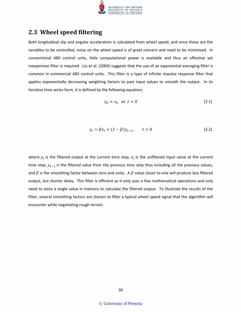
𝑦𝑡 = 𝛽𝑥𝑡 + (1 − 𝛽)𝑦𝑡−1, 𝑡 > 0 [2.2]

where 𝑦𝑡 is the filtered output at the current time step, 𝑥𝑡 is the unfiltered input value at the current

time step, 𝑦𝑡−1 is the filtered value from the previous time step thus including all the previous values,

and 𝛽 is the smoothing factor between zero and unity. A 𝛽 value closer to one will produce less filtered

output, but shorter delay. This filter is efficient as it only uses a few mathematical operations and only

need to store a single value in memory to calculate the filtered output. To illustrate the results of the

filter, several smoothing factors are chosen to filter a typical wheel speed signal that the algorithm will

encounter while negotiating rough terrain.


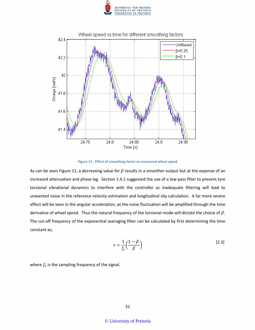
31

Figure 11: Effect of smoothing factor on measured wheel speed

As can be seen Figure 11, a decreasing value for 𝛽 results in a smoother output but at the expense of an

increased attenuation and phase lag. Section 1.4.1 suggested the use of a low pass filter to prevent tyre

torsional vibrational dynamics to interfere with the controller as inadequate filtering will lead to

unwanted noise in the reference velocity estimation and longitudinal slip calculation. A far more severe

effect will be seen in the angular acceleration, as the noise fluctuation will be amplified through the time

derivative of wheel speed. Thus the natural frequency of the torsional mode will dictate the choice of 𝛽.

The cut-off frequency of the exponential averaging filter can be calculated by first determining the time

constant as;

𝜏 =1𝑓𝑠�

1 − 𝛽 𝛽

� [2.3]

where 𝑓𝑠 is the sampling frequency of the signal.


32

The resulting cut-off, or cornering frequency is then calculated in Hz as;

𝑓𝑐 =1

2𝜋𝜏 [2.4]

From characterisation of the specific tyre used in this study, it is known that the torsional natural

frequency is at 31.1Hz and a 𝛽 value of 0.1 will result in a cut-off frequency of 17.7 Hz. Even though this

filter frequency is a factor two below the torsional natural frequency, the pass-band is still adequate to

allow all other important dynamics to be interpreted.

2.4 Reference velocity calculation To accurately estimate the linear velocity of the vehicle is of ultimate importance to the success of ABS,

since the calculation of longitudinal slip depends on the velocity of the vehicle. It is also used to

determine when the ABS should be switched off, since ABS is impractical at low speeds due to numerical

instability with the calculation of angular acceleration. During normal driving conditions, little

longitudinal slip is present between the rolling tyre and the stationary road and the no-slip assumption

is valid to calculate the vehicle velocity as:

𝑣 = 𝜔𝑟 [2.5]

However, during severe braking manoeuvres slip is significant and the no-slip assumption does not hold.

This leads to the problem that vehicle velocity cannot be calculated or measured directly since ABS does

not make use of any sensors other than the wheel speed sensors. At best, the velocity has to be

estimated by making certain assumptions and since the vehicle velocity is no longer directly calculated

or measured, it is referred to as the reference velocity of the vehicle. The following equation is used for

this purpose;

𝑣 = 𝑣𝑖 − 𝑅∆𝑡 [2.6]

where 𝑣𝑖 is the reference velocity in the previous time step, 𝑅 is the deceleration constant, and ∆𝑡 is the

time step size. In section 2.6, the calculation of angular and linear acceleration is explained. Should the

controller calculate an unrealistic deceleration value of more than 9.81, equation [2.6] is to be used

instead of equation [2.5]. The use of equation [2.6] implies the assumption that the vehicle is

decelerating at a constant rate, which is untrue since different friction coefficients, tyre force saturation


33

and fluctuation in ABS brake pressure will lead to fluctuating longitudinal force generation. The

deceleration value, 𝑅, represents the anticipated rate at which the vehicle can decelerate and is highly

dependent on road conditions. For high tractive surfaces it can be chosen as 𝜇𝑝𝑔, and will be true in

ideal conditions and with optimum ABS performance. In essence, the reference velocity is calculated by

equation [2.5] when the wheels are not slipping and with equation [2.6] when any amount of slip is

occurring. Naturally this will lead to discontinuities in the reference velocity when the calculation

thereof jumps between these two equations. These discontinuities will echo through the calculated slip

values and can cause the controller to function sub-optimally. This effect can be reduced somewhat

with well-tuned ABS thresholds and four wheel speed sensors that supply continuous information.

2.5 Longitudinal slip calculation Longitudinal slip is the control variable that requires a higher priority than angular acceleration, and thus

inaccurate calculation of this variable may severely degrade ABS performance. Longitudinal slip for each

wheel is calculated using the current angular velocity and vehicle velocity as;

𝜆 = 𝑣 − 𝜔𝑟

𝑣 [2.7]

where 𝜆 is the unitless longitudinal slip, 𝑣 is the reference velocity of the vehicle, 𝜔 is the angular

velocity of the concerned wheel and 𝑟 is the rolling radius of the tyre. The value of 𝑟 is chosen as the

undeflected radius of the tyre. This, on its own, is an important parameter to consider on rough roads

as the assumption of constant rolling radius can be very inaccurate. A slip threshold is chosen that is

slightly higher than the peak slip value at which the tyre produces maximum longitudinal force, since the

controller will react to keep the calculated slip below this threshold and the average will tend towards

the peak value.


34

2.6 Wheel angular acceleration The other variable that is controlled is the angular acceleration of each wheel. This is calculated more

easily than slip and reference velocity, but is more susceptible to noise since it is differentiated from the

measured angular velocity. Angular acceleration does not only form the basis of the Bosch control

algorithm, but is also used to calculate the current deceleration of the vehicle. The angular acceleration

of the wheel is calculated as;

𝛼 =𝜔𝑡 − 𝜔𝑡−𝑛

𝑛Δ𝑡 [2.8]

where 𝜔𝑡 is the current wheel speed and 𝜔𝑡−𝑛 is the wheel speed of the 𝑛’th previous time step. The 𝑛

variable is included to minimize the effect of noise amplification by differentiating over a larger time

step and should be chosen as a smaller number as it will introduce a time delay. The controller will react

according to the flowchart depicted in Figure 10 to keep the angular acceleration within the two defined

thresholds, but takes second priority to slip. As stated before, angular acceleration is also used to

determine whether or not to use equation [2.5] or [2.6]. For a free rolling tyre with no slippage, the

following equation holds;

𝑎0 = 𝛼𝑟 [2.9]

where 𝑎0 is the linear acceleration of the vehicle. Assuming a maximum static friction coefficient of

unity for the tyre-road contact and neglecting aerodynamics, 𝑎0 cannot be larger than 1g and would

imply that slippage is present, should it be calculated as such. In which case, equation {2.6} is to be used

for reference velocity calculation.


35

2.7 Intelligent ABS algorithms Although the scope of this study does not include intelligent algorithms, it is worth exploring the

fundamentals as all modern ABS algorithms incorporate a certain amount of intelligence in order to

adapt to the different terrains that the system might encounter. Two parameters are generally adapted

to optimise braking performance, namely the deceleration value 𝑅 and the slip threshold 𝜆. Successful

implementation will ensure that the reference velocity is always accurate and that the slip threshold is

always in close agreement with the peak slip value.

2.7.1 Deceleration constant adaptive Jiang & Gao (2000) describe a non-linear filter that estimates vehicle velocity by adapting the

deceleration value 𝑅 as the vehicle progresses through the ABS manoeuvre. This adapting algorithm will

adapt to the correct deceleration value even when the vehicle encounters multiple surfaces with

different friction coefficients during a single braking manoeuvre. It does so by inaccurately estimating

vehicle speed during initial wheel lock-up, and adjusting the deceleration value when the wheel speed

reaches a peak.

2.7.2 Slip adaptive To have the ABS algorithm adapt the slip threshold is the second step to ensuring that the system

performs at peak performance over a wide variety of terrains. The angular acceleration value is used to

select the slip threshold to be slightly greater than the peak slip value at which peak longitudinal force

occurs. Referring to the flow chart in Figure 10, the end of phase 2 signifies that the wheel is already

past its peak slip value and braking pressure should be released. Selecting the slip value at the start of

phase two is a good estimation of the peak slip value for the current terrain.

2.7.3 Other aids for ABS As mentioned in section 1.3.2, the use of GPS or accelerometers to aid ABS cannot be considered as the

classical Bosch algorithm. Such sensors will greatly improve the estimation of the reference velocity of

the vehicle, or completely eliminate the need for estimation at all. These sensors are common in

vehicles today, thus it is possible that it may be used as aid to ABS systems on commercial vehicles.

Friction coefficient estimation is another potentially important addition to the classic wheel speed

sensor algorithm. This will allow the controller to predict, rather than reacting to wheel lockup. Some

techniques include optical, vibrational or longitudinal slip measurements.


36

Chapter 3: Test Platform & ADAMS Model

Introduction This chapter describes the process of retrofitting a non-ABS test vehicle with ABS brake hardware,

developing an ABS controller based on an embedded computer, developing a vehicle dynamic model

suitable for simulating ABS operation on rough terrain and, finally, compare the correlation of the

results between vehicle tests and simulations.

3.1 Test platform The test vehicle that is used in this study is a 1997 Land Rover Defender 110 TDi. The Vehicle Dynamics

Group of the University of Pretoria has used this vehicle for the past ten years and several systems and

sensors have been added to the vehicle to facilitate effective testing. Some of these systems include a 4

state semi-active suspension system (4S4), an active anti-roll bar and both a steering and throttle driver

robot. The main sensors that are used in this study include wheel speed sensors, pressure transducers,

Inertial Navigation System (INS), and a wheel force transducer (WFT).

3.1.1 Suspension The vehicle is fitted with a four State Semi-active Suspension (4S4), developed by Els (2006). This

suspension system is capable of switching between four states (two spring stiffness and two damping

states on each strut) within 100ms. An arrangement of solenoid valves switches between small and

large pneumatic accumulators to change spring stiffness, while low and high damping states are

obtained by directing hydraulic flow through different orifices. The combination of low damping and

spring stiffness reduces vertical acceleration and yields a comfort suspension setup, while high damping

and spring stiffness yields reduced vehicle body roll and a handling setup is attained. The comfort setup

will be used throughout this study. Although not explored in this study, the semi-active suspension

system might prove to be a viable solution to the rough terrain braking problem.

3.1.2 Wheel speed sensors Since the Land Rover Defender only saw ABS fitted to the late Puma engine models from 2002 onwards,

ABS had to be installed on the test vehicle. There hasn’t been much change in the assembly of the


37

wheel hub between the earlier and the ABS equipped models, and the option to retrofit new hubs that

include the ABS pulse rings and sensor was explored. However, the more flexible and economic option

was chosen and four Festo inductive proximity sensors were installed. Literature suggests 60 pulses per

revolution to measure wheel speed on passenger vehicles (Bauer & Bosch 1999), and thus the pulse

rings were fabricated by drilling 60 holes into the brake disks to trigger the proximity switches. As

mentioned in section 1.4.1, terrain effects and vibration of the sensors alone is enough to hamper the

performance of ABS, thus special precaution was taken to fix the sensors rigidly. Although the pulses

from the proximity sensor switches are used directly for ABS control, the pulses were converted to

analogue wheel speeds using four Turck MS25-UI (Clearwater Tech 2015) frequency to voltage

converters. This allowed the analogue voltages to be sampled by the embedded data acquisition

computer.

3.1.3 Hydraulic system and brake hardware ABS requires only a modulator and a control unit other than the normal components used in

conventional hydraulic brakes. The test vehicle has separate hydraulic lines for the front wheels, but a

single line controlling the rear axle via the proportioning valve. Since ABS renders the proportioning

valve redundant due to the electronic control of brake pressure, separate hydraulic lines were installed

from the modulator to each calliper. Fortunately the vehicle has disk brakes installed as standard and

the Original Equipment Manufacturer (OEM) brake callipers are used with the ABS system. It seems that

the ABS fitted to the test vehicle uses the same callipers as the non-ABS vehicle. Pressure transducers

are installed as close to the callipers as possible to eliminate friction or compressibility effects that may

exist in the hydraulic line.

Four 40MPa Wika pressure transducers were installed to measure brake pressure using a self-

manufactured T-junction to facilitate both the transducer and a bleed nipple. The nipple ensures that

no air can get trapped inside the transducer’s cavity. To ensure adequate sealing of the hydraulic fluid,

corrosion resistant silicone o-rings were installed with the transducer.

Modern Land Rover Defenders are fitted with Wabco ABS modulators and the same model was installed

in the test vehicle. The ECU is located separately from the modulator in this model, while most other

modulators and ECUs are packaged as a single unit. This had the mayor benefit that a custom

embedded controller could be easily interfaced to the modulator.


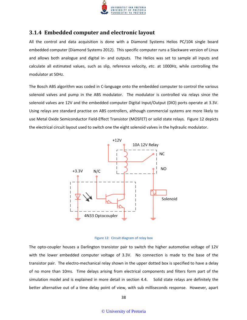
38

3.1.4 Embedded computer and electronic layout All the control and data acquisition is done with a Diamond Systems Helios PC/104 single board

embedded computer (Diamond Systems 2012). This specific computer runs a Slackware version of Linux

and allows both analogue and digital in- and outputs. The Helios was set to sample all inputs and

calculate all estimated values, such as slip, reference velocity, etc. at 1000Hz, while controlling the

modulator at 50Hz.

The Bosch ABS algorithm was coded in C-language onto the embedded computer to control the various

solenoid valves and pump in the ABS modulator. The modulator is controlled via relays since the

solenoid valves are 12V and the embedded computer Digital Input/Output (DIO) ports operate at 3.3V.

Using relays are standard practise on ABS controllers, although commercial systems are more likely to

use Metal Oxide Semiconductor Field-Effect Transistor (MOSFET) or solid state relays. Figure 12 depicts

the electrical circuit layout used to switch one the eight solenoid valves in the hydraulic modulator.

Figure 12: Circuit diagram of relay box

The opto-coupler houses a Darlington transistor pair to switch the higher automotive voltage of 12V

with the lower embedded computer voltage of 3.3V. No connection is made to the base of the

transistor pair. The electro-mechanical relay shown in the upper dotted box is specified to have a delay

of no more than 10ms. Time delays arising from electrical components and filters form part of the

simulation model and is explained in more detail in section 4.4. Solid state relays are definitely the

better alternative out of a time delay point of view, with sub milliseconds response. However, apart


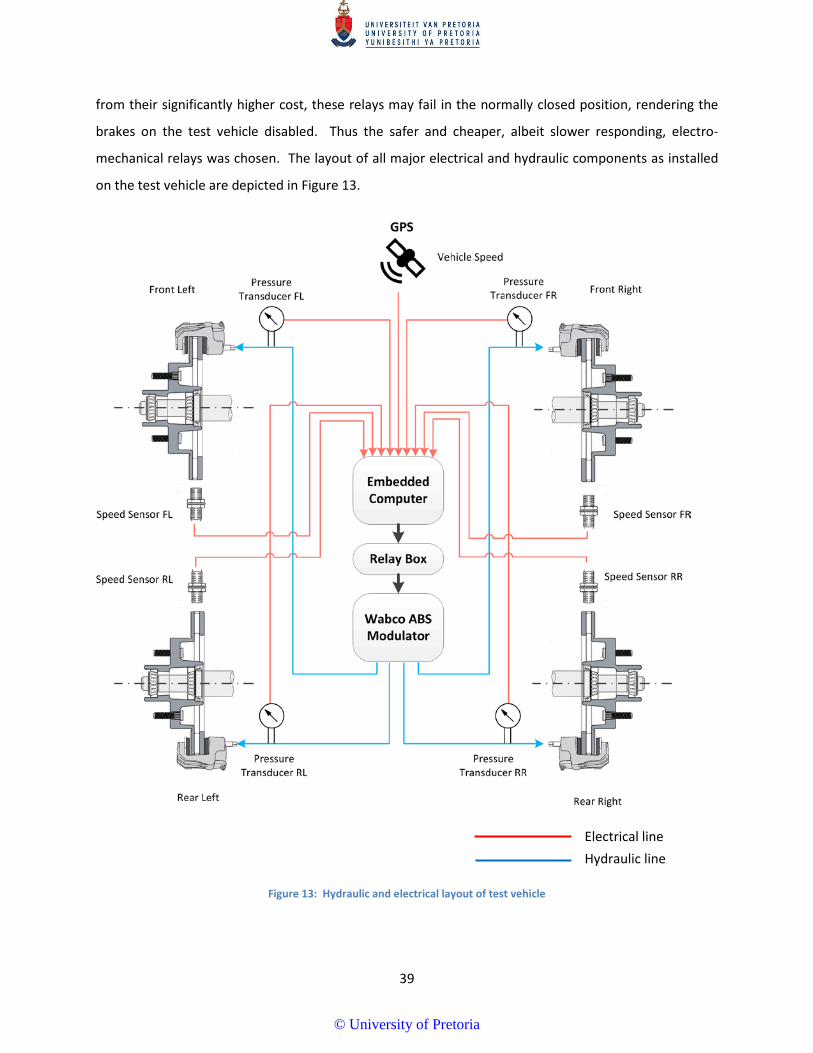
39

from their significantly higher cost, these relays may fail in the normally closed position, rendering the

brakes on the test vehicle disabled. Thus the safer and cheaper, albeit slower responding, electro-

mechanical relays was chosen. The layout of all major electrical and hydraulic components as installed

on the test vehicle are depicted in Figure 13.

Figure 13: Hydraulic and electrical layout of test vehicle

Hydraulic line Electrical line


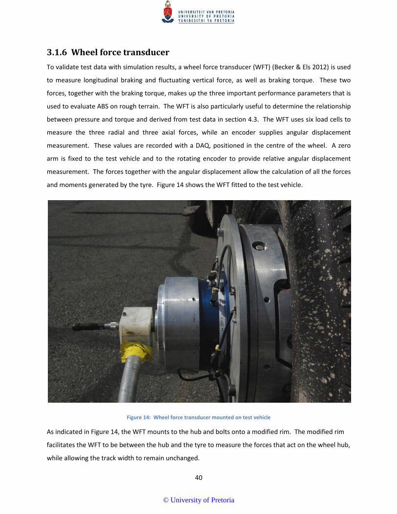
40

3.1.6 Wheel force transducer To validate test data with simulation results, a wheel force transducer (WFT) (Becker & Els 2012) is used

to measure longitudinal braking and fluctuating vertical force, as well as braking torque. These two

forces, together with the braking torque, makes up the three important performance parameters that is

used to evaluate ABS on rough terrain. The WFT is also particularly useful to determine the relationship

between pressure and torque and derived from test data in section 4.3. The WFT uses six load cells to

measure the three radial and three axial forces, while an encoder supplies angular displacement

measurement. These values are recorded with a DAQ, positioned in the centre of the wheel. A zero

arm is fixed to the test vehicle and to the rotating encoder to provide relative angular displacement

measurement. The forces together with the angular displacement allow the calculation of all the forces

and moments generated by the tyre. Figure 14 shows the WFT fitted to the test vehicle.

Figure 14: Wheel force transducer mounted on test vehicle

As indicated in Figure 14, the WFT mounts to the hub and bolts onto a modified rim. The modified rim

facilitates the WFT to be between the hub and the tyre to measure the forces that act on the wheel hub,

while allowing the track width to remain unchanged.


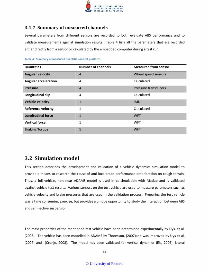
41

3.1.7 Summary of measured channels Several parameters from different sensors are recorded to both evaluate ABS performance and to

validate measurements against simulation results. Table 4 lists all the parameters that are recorded

either directly from a sensor or calculated by the embedded computer during a test run.

Table 4: Summary of measured quantities on test platform

Quantities Number of channels Measured from sensor

Angular velocity 4 Wheel speed sensors

Angular acceleration 4 Calculated

Pressure 4 Pressure transducers

Longitudinal slip 4 Calculated

Vehicle velocity 1 IMU

Reference velocity 1 Calculated

Longitudinal force 1 WFT

Vertical force 1 WFT

Braking Torque 1 WFT

3.2 Simulation model This section describes the development and validation of a vehicle dynamics simulation model to

provide a means to research the cause of anti-lock brake performance deterioration on rough terrain.

Thus, a full vehicle, nonlinear ADAMS model is used in co-simulation with Matlab and is validated

against vehicle test results. Various sensors on the test vehicle are used to measure parameters such as

vehicle velocity and brake pressures that are used in the validation process. Preparing the test vehicle

was a time consuming exercise, but provides a unique opportunity to study the interaction between ABS

and semi-active suspension.

The mass properties of the mentioned test vehicle have been determined experimentally by Uys, et al.

(2006). The vehicle has been modelled in ADAMS by Thoresson, (2007)and was improved by Uys et al.

(2007) and (Cronje, 2008). The model has been validated for vertical dynamics (Els, 2006), lateral


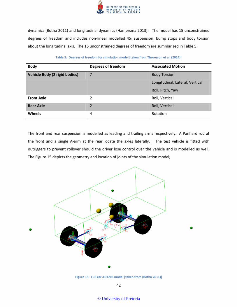
42

dynamics (Botha 2011) and longitudinal dynamics (Hamersma 2013). The model has 15 unconstrained

degrees of freedom and includes non-linear modelled 4S4 suspension, bump stops and body torsion

about the longitudinal axis. The 15 unconstrained degrees of freedom are summarized in Table 5.

Table 5: Degrees of freedom for simulation model [taken from Thoresson et al. (2014)]

Body Degrees of freedom Associated Motion

Vehicle Body (2 rigid bodies) 7 Body Torsion

Longitudinal, Lateral, Vertical

Roll, Pitch, Yaw

Front Axle 2 Roll, Vertical

Rear Axle 2 Roll, Vertical

Wheels 4 Rotation

The front and rear suspension is modelled as leading and trailing arms respectively. A Panhard rod at

the front and a single A-arm at the rear locate the axles laterally. The test vehicle is fitted with

outriggers to prevent rollover should the driver lose control over the vehicle and is modelled as well.

The Figure 15 depicts the geometry and location of joints of the simulation model;

Figure 15: Full car ADAMS model [taken from (Botha 2011)]


43

The green spheres in the figure are the outriggers that are modelled as masses, while the yellow spheres

are the passengers and driver. Note that the body is made up by two boxes that are connected with a

torsional spring to model the body torsion of the vehicle.

3.2.1 Suspension The 4S4 is modelled as a force in the ADAMS model. Gas volume dictates the spring stiffness, which can

be set to high or low by choosing one of two discrete volumes. The damping is set in relation to the

OEM dampers and two factors select either higher or lower damping than the baseline. These four

values yields a “ride comfort mode” with soft springs and low damping, and a “handling mode” with stiff

springs and high damping. A control system can automatically switch between “ride” and “handling”

modes, depending on what suspension setup is required for a particular scenario. The spring and

damping values, in conjunction with strut displacement and velocity are used by ADAMS to calculate the

suspension force. An automatic suspension control option is available where the running RMS of

vertical acceleration of the centre of mass is used to switch between handling and comfort mode, as is

the case with the test vehicle.

3.2.2 Driver model Since most of the experimental results in this study are straight line braking over rough terrain, a driver

model is necessary to ensure the vehicle drives in a straight line during simulations. Botha (2011)

implemented a combined yaw acceleration and lateral error driver model to steer the vehicle along a

desired path. By calculating the required yaw acceleration as a function of longitudinal velocity and

steer rate, and combining it with the current lateral position error, the steer rate of the vehicle is

determined. The desired yaw rate is defined to be at a defined preview distance point from the

vehicle’s position.

3.2.3 ABS Control Algorithm The same algorithm as explained in section 2.1 was coded as a Matlab interpreted function and used in

the Simulink environment to simulate with ADAMS via the co-simulation function. The algorithm uses

three states to control the output pressure to the brake callipers. The ADAMS model accepts brake

toque, so the pressure is converted to torque by using the measured pressure-torque relationship, as

explained in section 4.3. The basic layout in the Simulink environment is shown Figure 16.


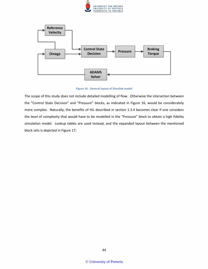
44

Figure 16: General layout of Simulink model

The scope of this study does not include detailed modelling of flow. Otherwise the interaction between

the “Control State Decision” and “Pressure” blocks, as indicated in Figure 16, would be considerately

more complex. Naturally, the benefits of HiL described in section 1.3.4 becomes clear if one considers

the level of complexity that would have to be modelled in the “Pressure” block to obtain a high fidelity

simulation model. Lookup tables are used instead, and the expanded layout between the mentioned

block sets is depicted in Figure 17;


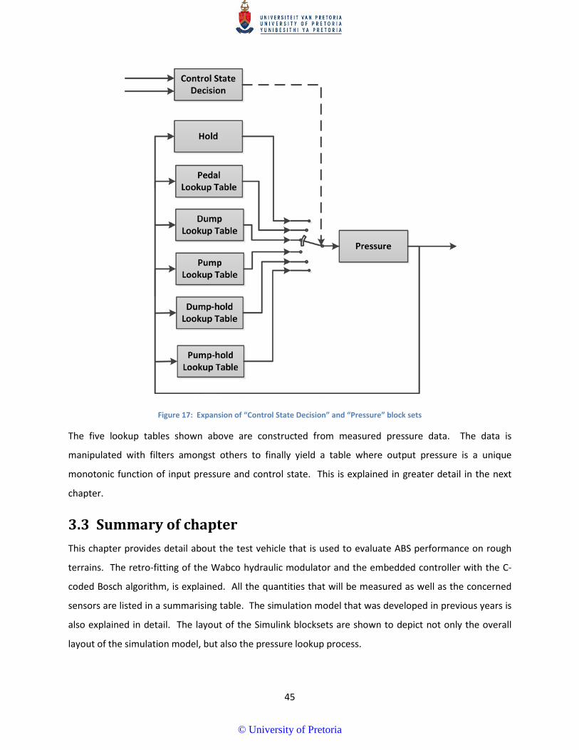
45

Figure 17: Expansion of “Control State Decision” and “Pressure” block sets

The five lookup tables shown above are constructed from measured pressure data. The data is

manipulated with filters amongst others to finally yield a table where output pressure is a unique

monotonic function of input pressure and control state. This is explained in greater detail in the next

chapter.

3.3 Summary of chapter This chapter provides detail about the test vehicle that is used to evaluate ABS performance on rough

terrains. The retro-fitting of the Wabco hydraulic modulator and the embedded controller with the C-

coded Bosch algorithm, is explained. All the quantities that will be measured as well as the concerned

sensors are listed in a summarising table. The simulation model that was developed in previous years is

also explained in detail. The layout of the Simulink blocksets are shown to depict not only the overall

layout of the simulation model, but also the pressure lookup process.


46

Chapter 4: Modelling of ABS

Introduction A data driven modelling approach, as explained in section 1.3.3, is used to simulate the ABS system in

this study. It follows that several lookup tables and measured delays form part of the Simulink model

that is used in co-simulation with ADAMS. The Simulink solver was set to solve at discrete time steps, in

this case 1 millisecond, to have the simulation model follow the same operation as the embedded

controller. The ABS control logic is implemented in Simulink as an interpreted function that determines

the Bosch phase to be converted to pressure. Look-up tables provide the pressure value for the next

iteration depending on the current value and Bosch phase. Finally, pressure is converted to brake

torque by using a linear relationship that is also drawn from measurements.

4.1 Assumptions The Bosch algorithm was modelled in Matlab as an interpreted function with several assumptions

already incorporated. The slip and angular acceleration thresholds are assumed to be constant and do

not vary with speed or road conditions. This is a shortcoming on the algorithm’s part as commercial ABS

algorithms are intelligent to adapt thresholds. All simulations and tests are done with the same

manoeuvre where the driver applied brakes in a panicked fashion and keeps the pedal actuated until the

vehicle comes to a complete standstill. The vehicle is kept in a straight line during all tests, and the

simulation model makes use of a driver model to ensure straight line braking.

To disregard temperature effects at the calliper may be a potentially risky assumption. Temperature will

introduce non-linearities that will otherwise not be captured. Friction coefficient of the brake pad is

heavily dependent on temperature and excessive braking will deteriorate brake performance. However,

Breuer & Bill (2008) suggests that this point, called brake fade, is only of concern if the temperature of

the system reaches 700 °C. The friction coefficient of the pad is thus assumed to be constant here. This

leads to a linear relationship between pressure and torque, which is modelled from measurements.

This study, unlike most ABS studies, will only be concerned with high traction surfaces. Since the main

focus will be on rough terrain, low traction roads will add unnecessary scope and diverge focus from the

rough road terrain problem. The Belgian Paving at Gerotek Test Facilities (Gerotek Test Facilities, 2015)

is used as the standard rough road input to both the simulation model and testing of the physical


47

system. This terrain is classified as a class D rough road as per ISO 8606 (International Organisation for

Standardisation 1995) and has already been profiled in a fine resolution for use in simulation (Becker

2008). This terrain consists of laid paving bricks that is assumed to excite the vehicle in a random

fashion over a wide range of frequencies, including the natural frequencies of the suspension system

and the tyres.

It is further assumed in the simulation that the modulator always has adequate pressure available and

that the pump supplies instantaneous pressure to the system. This will hold true on the test vehicle as

long as the pedal is actuated before the controller modulates the pressure, but might not be the case

with automated braking or distance following systems. The detailed modelling of the hydraulic system

is not performed in this study. The model follows a “black box” approach using lookup tables generated

from measured data.

4.2 Phase to Pressure

The ABS algorithm only performs control logic to decide on phases that have to be translated into

pressures. To simulate the pressure in Simulink, several lookup tables and delays are constructed from

measured data. The pressure lookup tables are constructed by using a test program that is installed on

the embedded computer. This program requires the user to apply the brakes as one would in a panic

stop scenario and then cycles through the dump, pump and hold states for each wheel to characterise

the pressure for each wheel individually. The modulator pump is switched on as soon as the first dump

state is initiated on the front left wheel. The resultant data is shown in Figure 18;


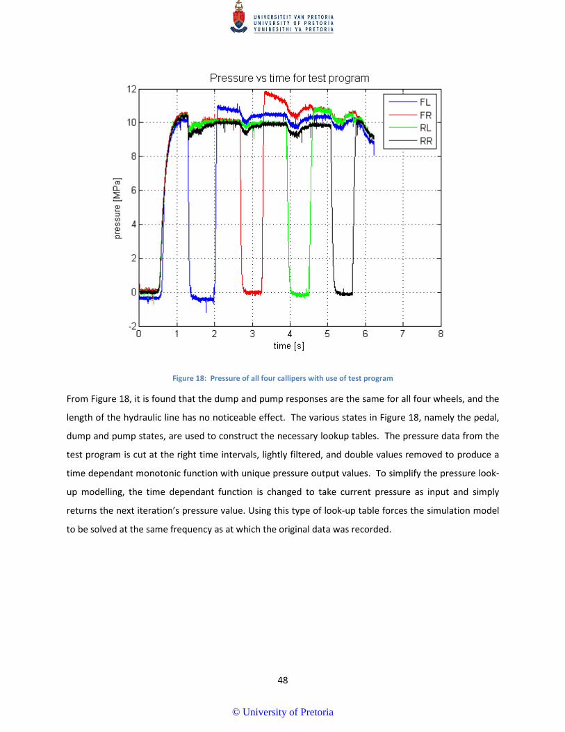
48

Figure 18: Pressure of all four callipers with use of test program

From Figure 18, it is found that the dump and pump responses are the same for all four wheels, and the

length of the hydraulic line has no noticeable effect. The various states in Figure 18, namely the pedal,

dump and pump states, are used to construct the necessary lookup tables. The pressure data from the

test program is cut at the right time intervals, lightly filtered, and double values removed to produce a

time dependant monotonic function with unique pressure output values. To simplify the pressure look-

up modelling, the time dependant function is changed to take current pressure as input and simply

returns the next iteration’s pressure value. Using this type of look-up table forces the simulation model

to be solved at the same frequency as at which the original data was recorded.


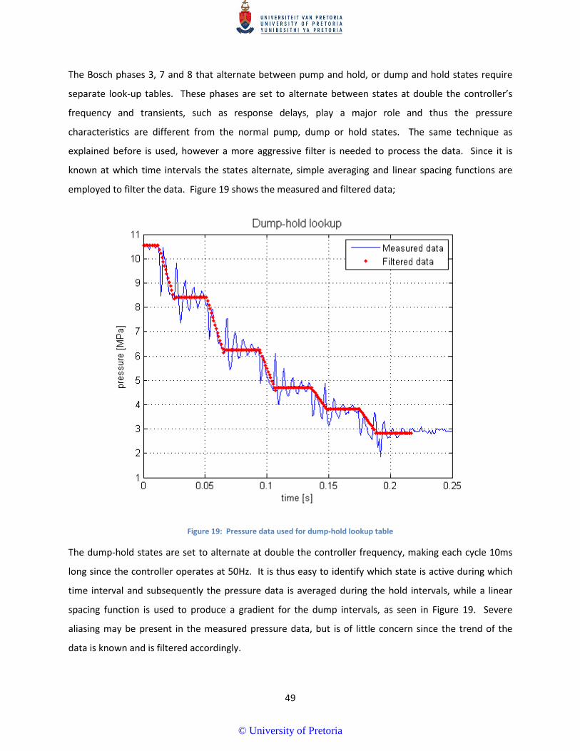
49

The Bosch phases 3, 7 and 8 that alternate between pump and hold, or dump and hold states require

separate look-up tables. These phases are set to alternate between states at double the controller’s

frequency and transients, such as response delays, play a major role and thus the pressure

characteristics are different from the normal pump, dump or hold states. The same technique as

explained before is used, however a more aggressive filter is needed to process the data. Since it is

known at which time intervals the states alternate, simple averaging and linear spacing functions are

employed to filter the data. Figure 19 shows the measured and filtered data;

Figure 19: Pressure data used for dump-hold lookup table

The dump-hold states are set to alternate at double the controller frequency, making each cycle 10ms

long since the controller operates at 50Hz. It is thus easy to identify which state is active during which

time interval and subsequently the pressure data is averaged during the hold intervals, while a linear

spacing function is used to produce a gradient for the dump intervals, as seen in Figure 19. Severe

aliasing may be present in the measured pressure data, but is of little concern since the trend of the

data is known and is filtered accordingly.


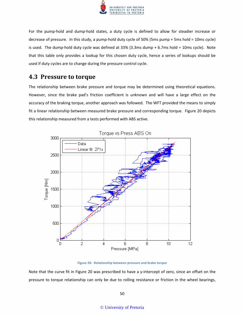
50

For the pump-hold and dump-hold states, a duty cycle is defined to allow for steadier increase or

decrease of pressure. In this study, a pump-hold duty cycle of 50% (5ms pump + 5ms hold = 10ms cycle)

is used. The dump-hold duty cycle was defined at 33% (3.3ms dump + 6.7ms hold = 10ms cycle). Note

that this table only provides a lookup for this chosen duty cycle, hence a series of lookups should be

used if duty cycles are to change during the pressure control cycle.

4.3 Pressure to torque The relationship between brake pressure and torque may be determined using theoretical equations.

However, since the brake pad’s friction coefficient is unknown and will have a large effect on the

accuracy of the braking torque, another approach was followed. The WFT provided the means to simply

fit a linear relationship between measured brake pressure and corresponding torque. Figure 20 depicts

this relationship measured from a tests performed with ABS active.

Figure 20: Relationship between pressure and brake torque

Note that the curve fit in Figure 20 was prescribed to have a y-intercept of zero, since an offset on the

pressure to torque relationship can only be due to rolling resistance or friction in the wheel bearings,


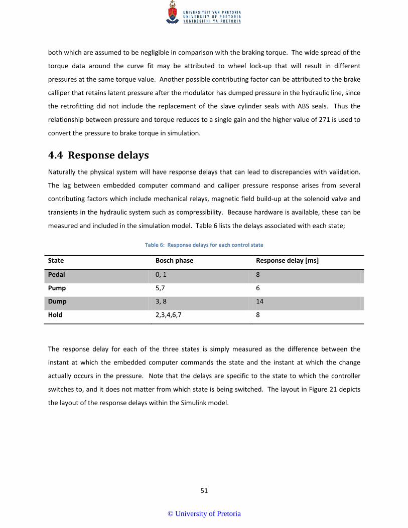
51

both which are assumed to be negligible in comparison with the braking torque. The wide spread of the

torque data around the curve fit may be attributed to wheel lock-up that will result in different

pressures at the same torque value. Another possible contributing factor can be attributed to the brake

calliper that retains latent pressure after the modulator has dumped pressure in the hydraulic line, since

the retrofitting did not include the replacement of the slave cylinder seals with ABS seals. Thus the

relationship between pressure and torque reduces to a single gain and the higher value of 271 is used to

convert the pressure to brake torque in simulation.

4.4 Response delays Naturally the physical system will have response delays that can lead to discrepancies with validation.

The lag between embedded computer command and calliper pressure response arises from several

contributing factors which include mechanical relays, magnetic field build-up at the solenoid valve and

transients in the hydraulic system such as compressibility. Because hardware is available, these can be

measured and included in the simulation model. Table 6 lists the delays associated with each state;

Table 6: Response delays for each control state

State Bosch phase Response delay [ms]

Pedal 0, 1 8

Pump 5,7 6

Dump 3, 8 14

Hold 2,3,4,6,7 8

The response delay for each of the three states is simply measured as the difference between the

instant at which the embedded computer commands the state and the instant at which the change

actually occurs in the pressure. Note that the delays are specific to the state to which the controller

switches to, and it does not matter from which state is being switched. The layout in Figure 21 depicts

the layout of the response delays within the Simulink model.


52

Figure 21: Layout of response delays in Simulink model

The values given in Figure 21 were measured from test data as an initial guess and tuned until the

respective quantities from the simulation results, such as slip and angular acceleration, showed good

correlation with test data. It was mentioned before in section 2.1 that the use of the “dump-hold”

states during phase 3 is because of a slow acting controller. Considering Figure 21, it can be seen that

the combined delays of 40ms and 80ms for the slip quantity will result in the controller reacting a total

of 120ms too slow during the 3rd phase and the controller will decrease the pressure far below what is

necessary to bring the wheel to acceptable slip levels. Thus, the use of the “dump” state in phase 3

resulted in a very long stopping distances and the implementation of the “dump-hold” alternating states

was used as a countermeasure.

4.5 Chapter summary This chapter describes the process that was followed to generate lookup tables from measured data in

an attempt to model the hydraulic modulator as a “black-box”. Five tables are constructed for each of

the five different states that is prescribed by the algorithm, namely pedal, pump, dump, dump-hold,

pump-hold. The lookup tables are constructed such that the pressure for the next simulation step is

dependent on the current pressure value, forcing the simulation to be performed at the same frequency

as which the test pressures were recorded.


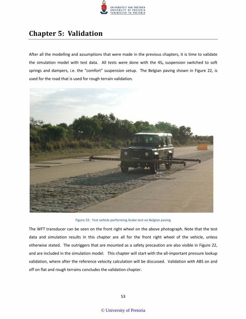
53

Chapter 5: Validation

After all the modelling and assumptions that were made in the previous chapters, it is time to validate

the simulation model with test data. All tests were done with the 4S4 suspension switched to soft

springs and dampers, i.e. the “comfort” suspension setup. The Belgian paving shown in Figure 22, is

used for the road that is used for rough terrain validation.

Figure 22: Test vehicle performing brake test on Belgian paving

The WFT transducer can be seen on the front right wheel on the above photograph. Note that the test

data and simulation results in this chapter are all for the front right wheel of the vehicle, unless

otherwise stated. The outriggers that are mounted as a safety precaution are also visible in Figure 22,

and are included in the simulation model. This chapter will start with the all-important pressure lookup

validation, where after the reference velocity calculation will be discussed. Validation with ABS on and

off on flat and rough terrains concludes the validation chapter.


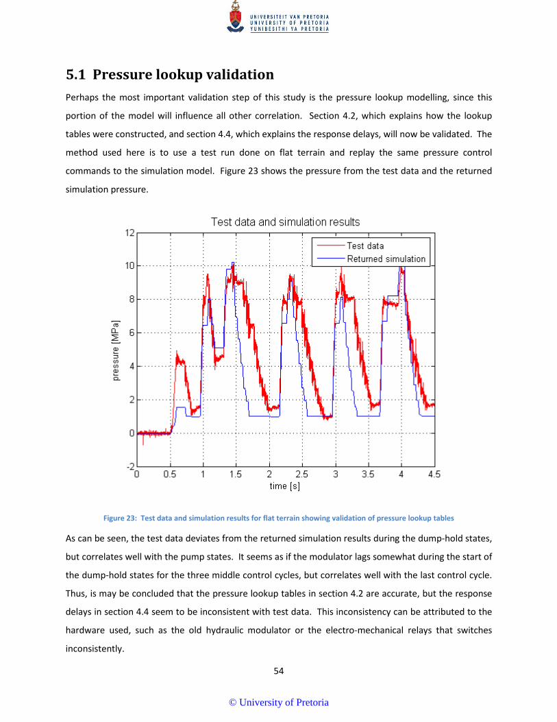
54

5.1 Pressure lookup validation Perhaps the most important validation step of this study is the pressure lookup modelling, since this

portion of the model will influence all other correlation. Section 4.2, which explains how the lookup

tables were constructed, and section 4.4, which explains the response delays, will now be validated. The

method used here is to use a test run done on flat terrain and replay the same pressure control

commands to the simulation model. Figure 23 shows the pressure from the test data and the returned

simulation pressure.

Figure 23: Test data and simulation results for flat terrain showing validation of pressure lookup tables

As can be seen, the test data deviates from the returned simulation results during the dump-hold states,

but correlates well with the pump states. It seems as if the modulator lags somewhat during the start of

the dump-hold states for the three middle control cycles, but correlates well with the last control cycle.

Thus, is may be concluded that the pressure lookup tables in section 4.2 are accurate, but the response

delays in section 4.4 seem to be inconsistent with test data. This inconsistency can be attributed to the

hardware used, such as the old hydraulic modulator or the electro-mechanical relays that switches

inconsistently.


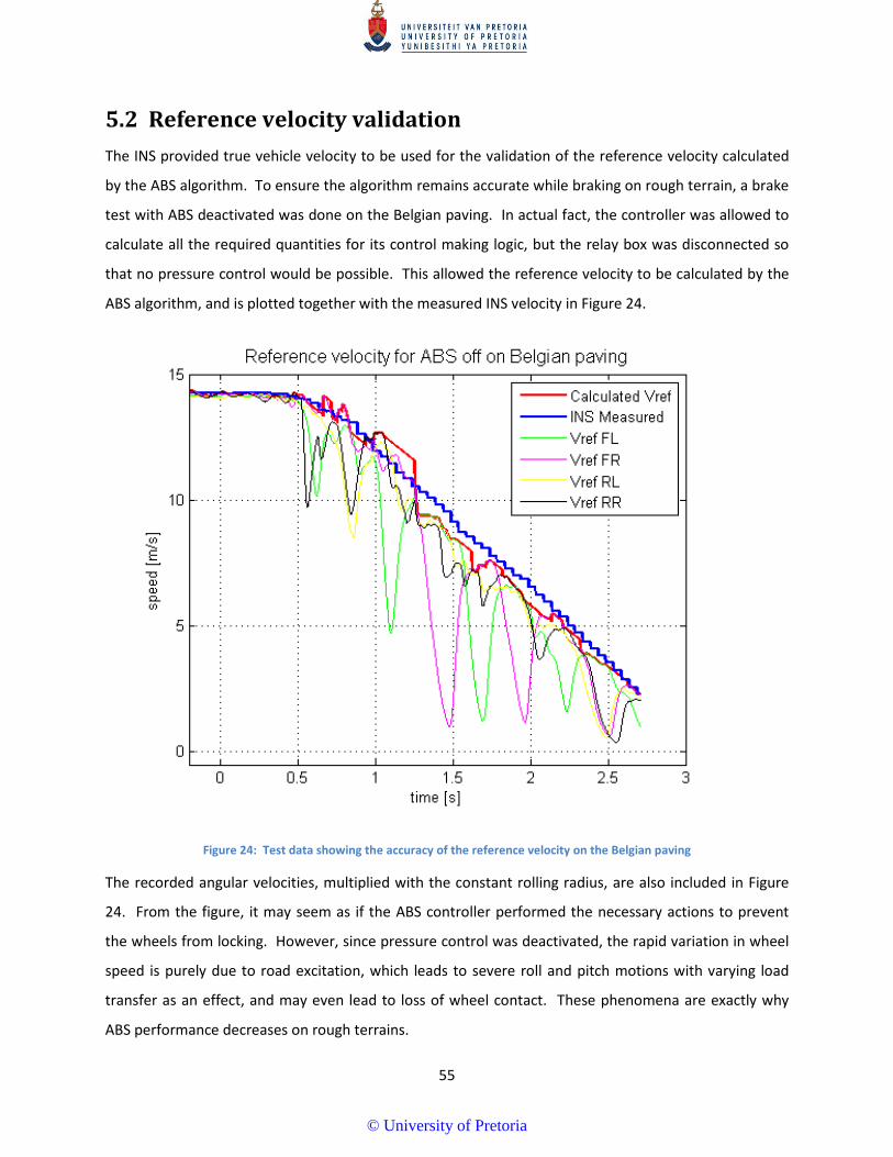
55

5.2 Reference velocity validation The INS provided true vehicle velocity to be used for the validation of the reference velocity calculated

by the ABS algorithm. To ensure the algorithm remains accurate while braking on rough terrain, a brake

test with ABS deactivated was done on the Belgian paving. In actual fact, the controller was allowed to

calculate all the required quantities for its control making logic, but the relay box was disconnected so

that no pressure control would be possible. This allowed the reference velocity to be calculated by the

ABS algorithm, and is plotted together with the measured INS velocity in Figure 24.

Figure 24: Test data showing the accuracy of the reference velocity on the Belgian paving

The recorded angular velocities, multiplied with the constant rolling radius, are also included in Figure

24. From the figure, it may seem as if the ABS controller performed the necessary actions to prevent

the wheels from locking. However, since pressure control was deactivated, the rapid variation in wheel

speed is purely due to road excitation, which leads to severe roll and pitch motions with varying load

transfer as an effect, and may even lead to loss of wheel contact. These phenomena are exactly why

ABS performance decreases on rough terrains.


56

Figure 24 draws a clear illustration of how the largest 𝑉𝑟𝑒𝑓 quantity is taken as the reference velocity of

the vehicle by the ABS algorithm while the wheels that are close to lockup are rejected. The flaws in the

estimation can also be seen however, as in the case of the two small bumps between 0.5s and 1.0s,

where faster than actual wheel speeds, perhaps from sensor noise or vibration, are chosen for 𝑉𝑟𝑒𝑓

calculation. The straight 𝑉𝑟𝑒𝑓 line segment between 1.0s and 1.5s shows how the algorithm detects

that no speed sensor provides accurate information and uses the linear deceleration formula to

calculate 𝑉𝑟𝑒𝑓.

In conclusion, although somewhat crude and simple, it can thus be seen that the ABS algorithm

calculates an accurate reference velocity when compared to the measured INS velocity, with a

maximum absolute relative error of 18.4% and a mean of 5.6%.

5.3 Flat road validation The simulation model is first validated on a high traction flat road. Minimal disturbances are present to

provide a benchmark from which the performance can be evaluated. Thresholds for both simulation

and test are set as -50 and 50 𝑟𝑎𝑑/𝑠2 for the minimum and maximum angular acceleration and 0.15 for

slip. The driver of the test vehicle performed a panicked stop at a speed of 60km/h and kept the vehicle

as straight as possible during the manoeuvre. Figure 25 shows the test data vs. the simulation results

for the front right wheel;


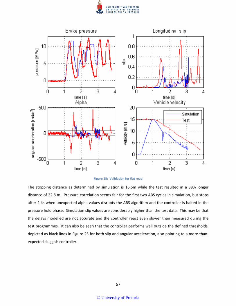
57

Figure 25: Validation for flat road

The stopping distance as determined by simulation is 16.5m while the test resulted in a 38% longer

distance of 22.8 m. Pressure correlation seems fair for the first two ABS cycles in simulation, but stops

after 2.4s when unexpected alpha values disrupts the ABS algorithm and the controller is halted in the

pressure hold phase. Simulation slip values are considerably higher than the test data. This may be that

the delays modelled are not accurate and the controller react even slower than measured during the

test programmes. It can also be seen that the controller performs well outside the defined thresholds,

depicted as black lines in Figure 25 for both slip and angular acceleration, also pointing to a more-than-

expected sluggish controller.


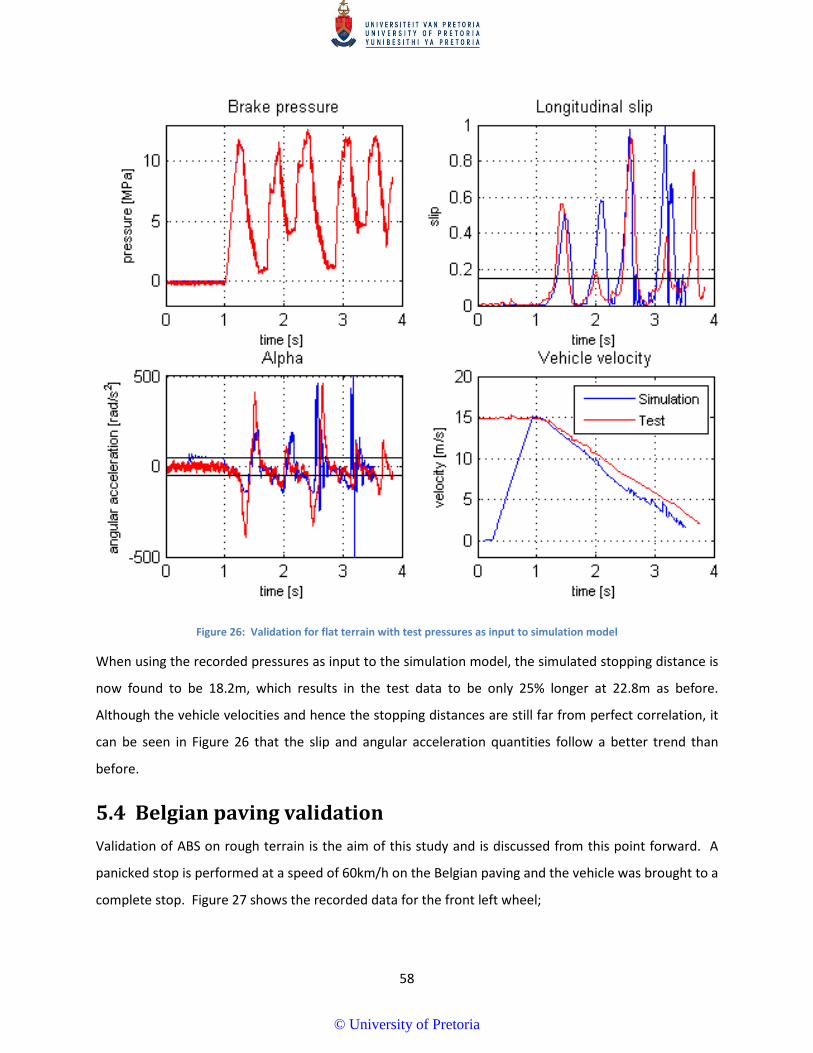
58

Figure 26: Validation for flat terrain with test pressures as input to simulation model

When using the recorded pressures as input to the simulation model, the simulated stopping distance is

now found to be 18.2m, which results in the test data to be only 25% longer at 22.8m as before.

Although the vehicle velocities and hence the stopping distances are still far from perfect correlation, it

can be seen in Figure 26 that the slip and angular acceleration quantities follow a better trend than

before.

5.4 Belgian paving validation Validation of ABS on rough terrain is the aim of this study and is discussed from this point forward. A

panicked stop is performed at a speed of 60km/h on the Belgian paving and the vehicle was brought to a

complete stop. Figure 27 shows the recorded data for the front left wheel;


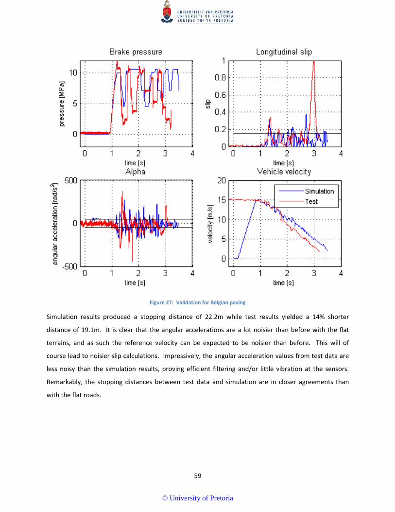
59

Figure 27: Validation for Belgian paving

Simulation results produced a stopping distance of 22.2m while test results yielded a 14% shorter

distance of 19.1m. It is clear that the angular accelerations are a lot noisier than before with the flat

terrains, and as such the reference velocity can be expected to be noisier than before. This will of

course lead to noisier slip calculations. Impressively, the angular acceleration values from test data are

less noisy than the simulation results, proving efficient filtering and/or little vibration at the sensors.

Remarkably, the stopping distances between test data and simulation are in closer agreements than

with the flat roads.


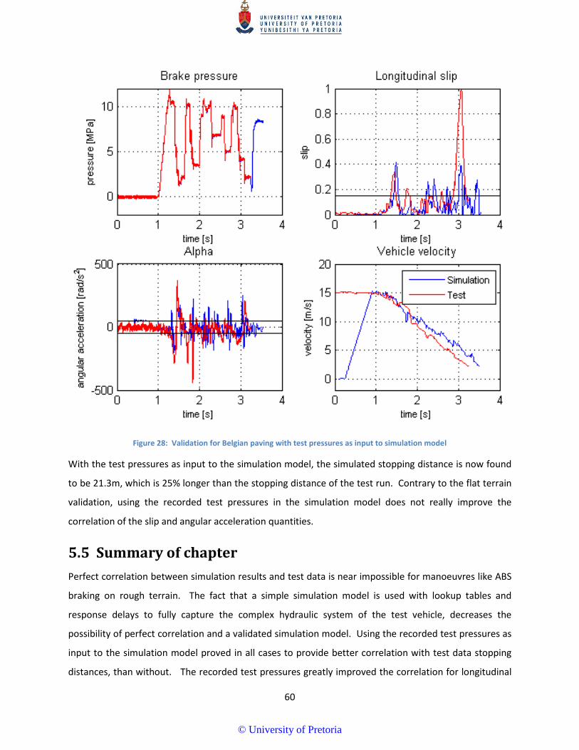
60

Figure 28: Validation for Belgian paving with test pressures as input to simulation model

With the test pressures as input to the simulation model, the simulated stopping distance is now found

to be 21.3m, which is 25% longer than the stopping distance of the test run. Contrary to the flat terrain

validation, using the recorded test pressures in the simulation model does not really improve the

correlation of the slip and angular acceleration quantities.

5.5 Summary of chapter Perfect correlation between simulation results and test data is near impossible for manoeuvres like ABS

braking on rough terrain. The fact that a simple simulation model is used with lookup tables and

response delays to fully capture the complex hydraulic system of the test vehicle, decreases the

possibility of perfect correlation and a validated simulation model. Using the recorded test pressures as

input to the simulation model proved in all cases to provide better correlation with test data stopping

distances, than without. The recorded test pressures greatly improved the correlation for longitudinal


61

slip and angular acceleration on flat terrain, while it did not improve the situation for rough terrain

substantially.

The aim of this study was to create a simulation model that can be used to evaluate the performance of

ABS on rough terrain, and explore possible solutions to the problem. Unfortunately, it cannot be

concluded that the simulation model is validated in any sense. However, the retrofitted ABS system on

the test vehicle seem to perform adequately, even on rough terrain, and a combination of the

simulation model together with the test vehicle might still prove as a useful tool for ABS research.


62

Chapter 6: Results

This chapter is focused on the discussion of increased stopping distance on rough terrain. First, the

simulation results for both flat and rough terrain will be compared where after the test data for the two

terrains will be discussed. Note that the test data and simulation results used here are the same as in

chapter 5, however now the comparison is made between flat and rough terrain to prove the increase in

stopping distance with ABS systems, and not between simulation and real world to prove a validated

model. This provides a comparative method where all other discrepancies are kept constant and the

terrain is the only parameter that changes.

6.1 Deterioration of performance using simulation model Although not fully validated, using a simulation model to evaluate ABS performance was the aim of this

study and will be used first. A comparison is now made between the stopping distance of ABS on rough

vs. flat terrain, using the same results and test data from before. Note that only simulation results are

concerned for Figure 29.


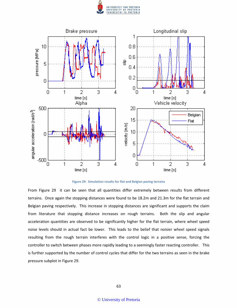
63

Figure 29: Simulation results for flat and Belgian paving terrains

From Figure 29 it can be seen that all quantities differ extremely between results from different

terrains. Once again the stopping distances were found to be 18.2m and 21.3m for the flat terrain and

Belgian paving respectively. This increase in stopping distances are significant and supports the claim

from literature that stopping distance increases on rough terrains. Both the slip and angular

acceleration quantities are observed to be significantly higher for the flat terrain, where wheel speed

noise levels should in actual fact be lower. This leads to the belief that noisier wheel speed signals

resulting from the rough terrain interferes with the control logic in a positive sense, forcing the

controller to switch between phases more rapidly leading to a seemingly faster reacting controller. This

is further supported by the number of control cycles that differ for the two terrains as seen in the brake

pressure subplot in Figure 29.


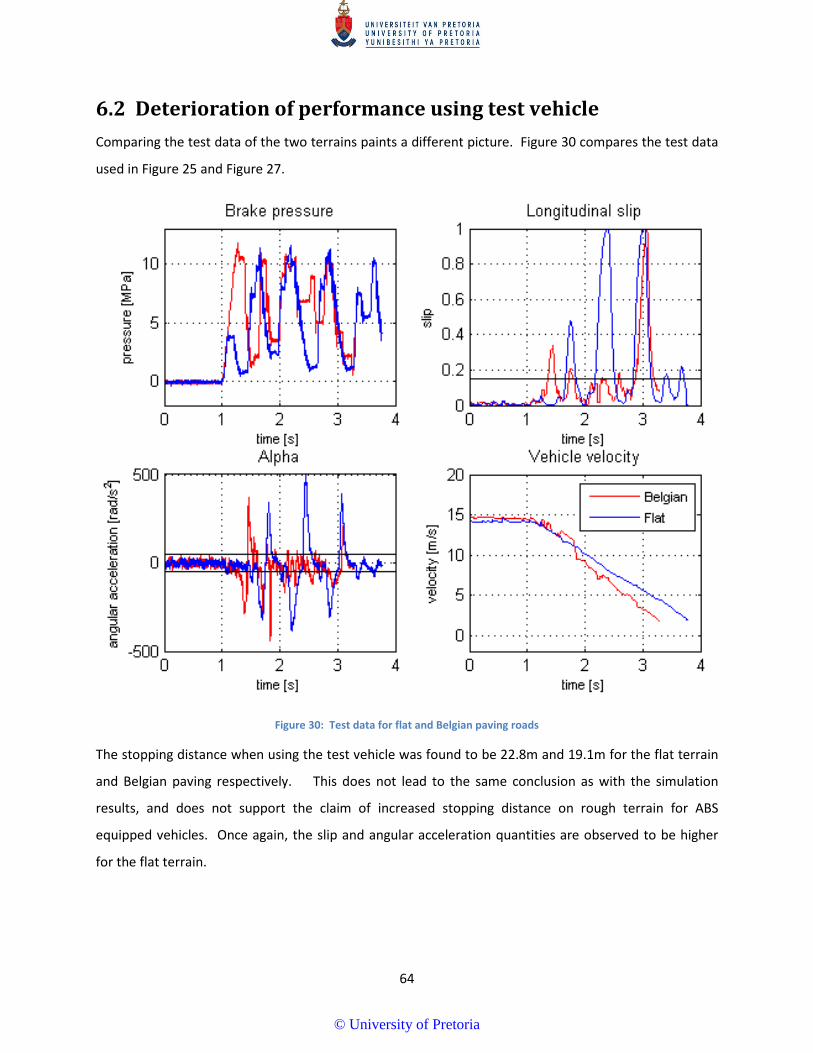
64

6.2 Deterioration of performance using test vehicle Comparing the test data of the two terrains paints a different picture. Figure 30 compares the test data

used in Figure 25 and Figure 27.

Figure 30: Test data for flat and Belgian paving roads

The stopping distance when using the test vehicle was found to be 22.8m and 19.1m for the flat terrain

and Belgian paving respectively. This does not lead to the same conclusion as with the simulation

results, and does not support the claim of increased stopping distance on rough terrain for ABS

equipped vehicles. Once again, the slip and angular acceleration quantities are observed to be higher

for the flat terrain.


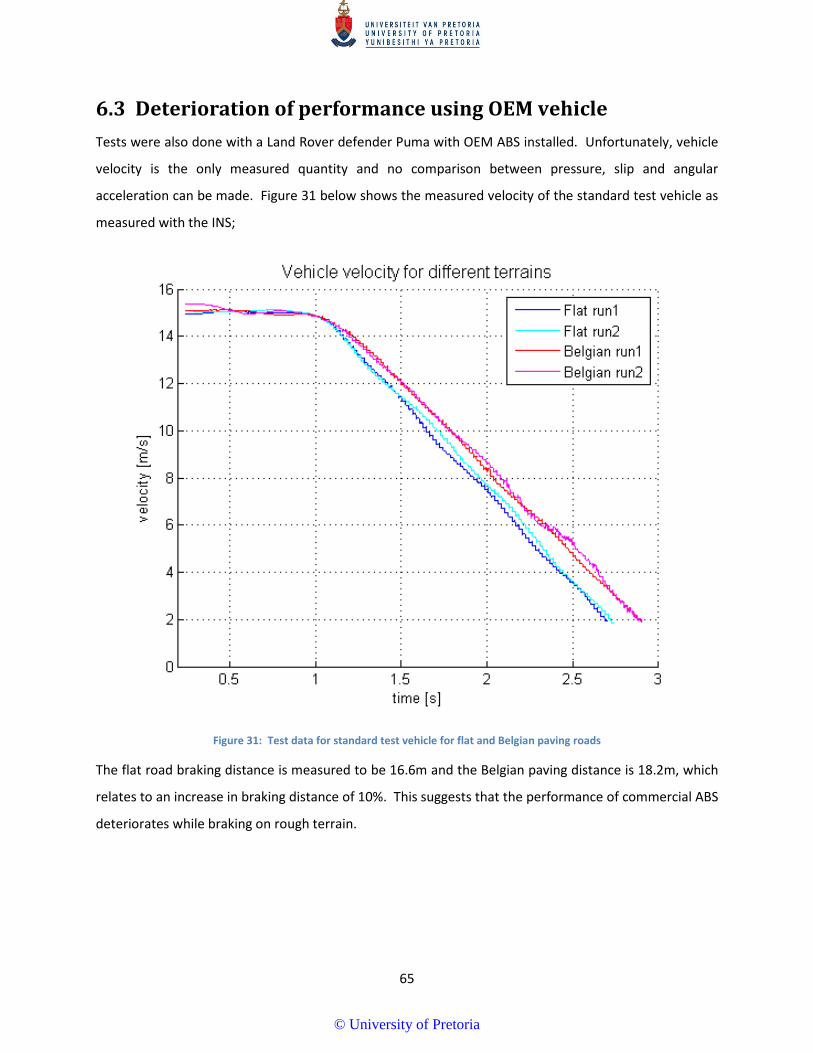
65

6.3 Deterioration of performance using OEM vehicle Tests were also done with a Land Rover defender Puma with OEM ABS installed. Unfortunately, vehicle

velocity is the only measured quantity and no comparison between pressure, slip and angular

acceleration can be made. Figure 31 below shows the measured velocity of the standard test vehicle as

measured with the INS;

Figure 31: Test data for standard test vehicle for flat and Belgian paving roads

The flat road braking distance is measured to be 16.6m and the Belgian paving distance is 18.2m, which

relates to an increase in braking distance of 10%. This suggests that the performance of commercial ABS

deteriorates while braking on rough terrain.


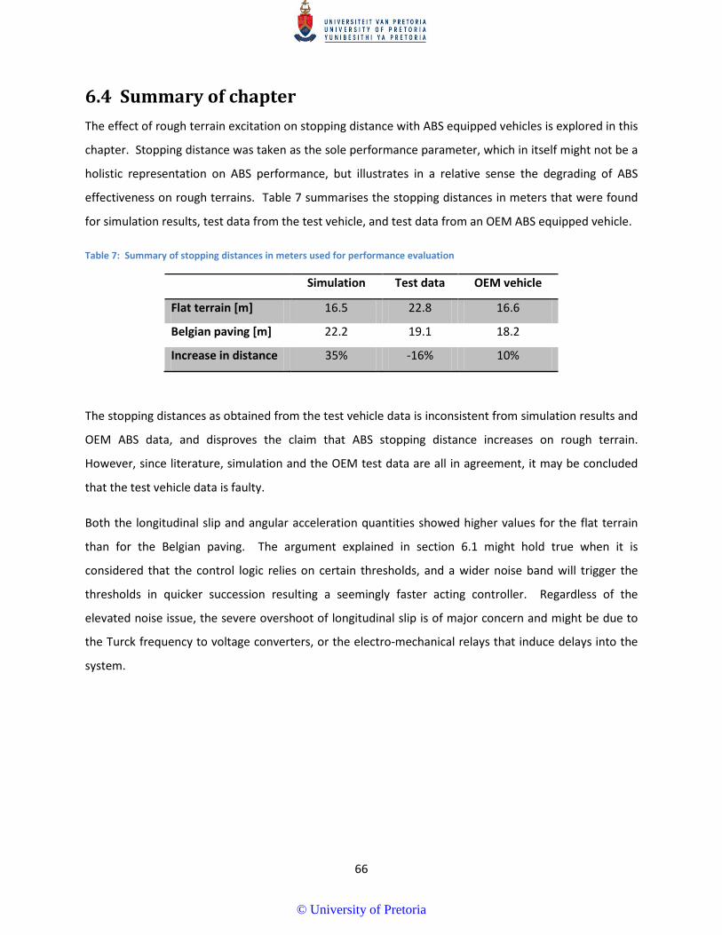
66

6.4 Summary of chapter The effect of rough terrain excitation on stopping distance with ABS equipped vehicles is explored in this

chapter. Stopping distance was taken as the sole performance parameter, which in itself might not be a

holistic representation on ABS performance, but illustrates in a relative sense the degrading of ABS

effectiveness on rough terrains. Table 7 summarises the stopping distances in meters that were found

for simulation results, test data from the test vehicle, and test data from an OEM ABS equipped vehicle.

Table 7: Summary of stopping distances in meters used for performance evaluation

Simulation Test data OEM vehicle

Flat terrain [m] 16.5 22.8 16.6

Belgian paving [m] 22.2 19.1 18.2

Increase in distance 35% -16% 10%

The stopping distances as obtained from the test vehicle data is inconsistent from simulation results and

OEM ABS data, and disproves the claim that ABS stopping distance increases on rough terrain.

However, since literature, simulation and the OEM test data are all in agreement, it may be concluded

that the test vehicle data is faulty.

Both the longitudinal slip and angular acceleration quantities showed higher values for the flat terrain

than for the Belgian paving. The argument explained in section 6.1 might hold true when it is

considered that the control logic relies on certain thresholds, and a wider noise band will trigger the

thresholds in quicker succession resulting a seemingly faster acting controller. Regardless of the

elevated noise issue, the severe overshoot of longitudinal slip is of major concern and might be due to

the Turck frequency to voltage converters, or the electro-mechanical relays that induce delays into the

system.


67

Chapter 7: Conclusion and Recommendations

A test vehicle was prepared with a retrofitted Anti-lock Braking System to research the deterioration of

ABS performance on rough terrain. The Bosch ABS algorithm was implemented in C-language on an

embedded computer to control an off-the-shelf hydraulic modulator by measuring wheel speed and

calculating the reference velocity of the vehicle. Pressure sensors and an Inertial Navigation System

provided the means to evaluate braking performance and validate a simulation model.

A data-driven simulation model using pressure lookup tables and response delays was built from test

data obtained from the physical system. The detailed mechanics of the Bosch algorithm and the

implementation thereof in the simulation model was explained. A validated FTire tyre model was used

in the multi-body dynamics software package ADAMS, while a Matlab/Simulink co-simulation provided

the pressure control.

The validation was not as successful as anticipated and poor correlation across all quantities was

observed when the simulation model was set to run independently from test data input. Correlation

between simulation results and test data was slightly better for flat terrains when the recorded pressure

data was used as input to the simulation model. Test data was also obtained with an Original

Equipment Manufacturer ABS vehicle to draw a clear comparison for stopping distances between the

retrofitted test vehicle and a commercially available system. Although the OEM vehicle performed

considerably better on flat terrain, the test vehicle proved to have a comparable stopping distance on

rough terrain.

Both the test data from the OEM vehicle and the simulation model supported the claim from literature

that stopping distance increases on rough terrain for ABS equipped vehicles. This was contradicted by

the test data from the test vehicle. It was argued that amplified noise resulting from the rough terrain

excitation results in the thresholds being triggered in rapid succession and ultimately leads to seemingly

faster controller. In the case with a flat terrain braking manoeuvre, the delays introduced into the

system by the use of slow frequency to voltage converters and electro-mechanical relays, causes the

slow controller to severely overshoot on the slip and angular acceleration quantities.


68

Several factors contributed to the ultimate inaccuracies of the simulation model and poor test data.

Most of these factors are solvable and should be attended to before further research is attempted. The

list below is the factors that have been identified as challenges to the outcome of this study;

I. More attention should be given to the implementation of wheel speed sensors and the OEM

hardware should be considered. This will reduce measurement noise and allow for a test

vehicle that is closer than OEM vehicles.

II. The use of solid-state relays may also minimise the lag between command signal and valve

switching. In addition, the Turck frequency to voltage converters should be replaced with a

faster acting solution, such as a dedicated microcontroller running at MHz sampling frequencies.

III. The implementation of (I) and (II) will lead to a faster acting controller which will result in less

overshoot in both the longitudinal slip and angular acceleration quantities.

IV. The modelling method of pressure lookup tables allows only for a fixed duty cycle for the pump-

hold and dump-hold states. Thus, if variable duty cycles are to be used, a whole series of lookup

tables needs to be constructed, or an alternative method of pressure modelling should be

explored, such as Hardware-in-the-Loop.


69

References

Adcox, J., Ayalew, B., Rhyne, T., Cron, S. & Knauff, M., 2013. Experimental Investigation of Tire Torsional Dynamics on the Performance of an Anti-Lock Braking System. In ASME 2013 International Design Engineering Technical Conferences and Computers and Information in Engineering Conference. pp. V001T01A028–V001T01A028.

Aly, A.A., Zeidan, E.-S., Hamed, A. & Salem, F., 2011. An antilock-braking systems (ABS) control: A technical review. Intelligent Control and Automation, 2(03), p.186.

Antoine, R.S., Jansen, S.T.H., Verhoeff, L., Cremers, R., Schmeitz, A.J.C. & Besselink, I.J.M., 2005. MF-Swift simulation study using benchmark data. International Journal of Vehicle Mechanics and Mobility.

Arrigoni, S., Cheli, F., Sabbioni, E. & Gavardi, P., 2015. Influence of tyre characteristics on ABS performance. In International Tyre Colloquium, 4th, 2015, Guildford, United Kingdom.

Bauer, H. & Bosch, R., 1999. Driving-safety systems: new electronic stability program ESP, SAE International.

Becker, C.M., 2008. Profiling of rough terrain. Unpublished MEng thesis. University of Pretoria, Pretoria, South Africa. Available at: http://repository.up.ac.za/handle/2263/31741.

Becker, C.M. & Els, P.S., 2011. Modal analysis on a large off-road tyre using Scanning Laser Vibrometry. In 17th International Conference of the ISTVS.

Becker, C.M. & Els, P.S., 2012. Wheel Force Transducer Measurements on a Vehicle in Transit. In Proceedings of the 12th European Regional Conference of the ISTVS. Pretoria, South Africa.

Bhivate, P., 2011. Modelling & development of antilock braking system. Unpublished BTech thesis. National Institute of Technology, Rourkela, India. Available at: http://ethesis.nitrkl.ac.in/2644/1/.

Blundell, M. & Harty, D., 2004. The multibody systems approach to vehicle dynamics, Elsevier.

Botha, T.R., 2011. High Speed Autonomous Off-Road Vehicle Steering. Unpublished MEng thesis. University of Pretoria, Pretoria, South Africa. Available at: http://repository.up.ac.za/handle/2263/31741.

Breuer, B. & Bill, K.H., 2008. Brake technology handbook, Warrendale, PA: SAE International.

Clearwater Tech, 2015. TURCK MS25-UI Digital to Analog Converters. Available at: http://www.clrwtr.com/PDF/TURCK/TURCK-Digital-Analog-Converters.pdf [Accessed May 23, 2015].

Cronje, P.H., 2008. Improving off-road vehicle handling using an active anti-roll bar. Unpublished MEng thesis, University of Pretoria. Available at: http://repository.up.ac.za/handle/2263/31741.


70

Day, T.D. & Roberts, S.G., 2002. A simulation model for vehicle braking systems fitted with ABS, No. 2002-01-0559. SAE Technical Paper.

Diamond Systems, 2012. Helios single board computer. Available at: http://www.diamondsystems.com/files/binaries/Helios User Manual.pdf [Accessed May 26, 2015].

Els, P.S., 2006. The ride comfort vs. handling compromise for off-road vehicles. Unpublished PhD thesis. University of Pretoria, Pretoria, South Africa. Available at: http://repository.up.ac.za/handle/2263/31741.

Eriksson, T., 2014. Co-Simulation of Full Vehicle Model in Adams and Anti-Lock Brake System Model in Simulink. Unpublished master’s thesis. Chalmers University of Technology. Available at: publications.lib.chalmers.se/records/fulltext/199941/199941.pdf.

Forkenbrock, G., Flick, M. & Garrott, W.R., 1999. A comprehensive light vehicle antilock brake system test track performance evaluation, No. 2002-01-0559. SAE Technical Paper.

Gerotek Test Facilities, 2015. . Available at: http://www.armscordi.com/SubSites/Gerotek1/Gerotek01_landing.asp [Accessed February 28, 2015].

Gillespie, T.D., 1999. Fundamentals of Vehicle dynamics, Warrendale, PA: SAE International.

Gipser, M., 1999. FTire , a New Fast Tire Model for Ride Comfort Simulations. In International ADAMS User Conference. Berlin, Germany, pp. 1–11.

Hamersma, H., 2013. Longitudinal vehicle dynamics control for improved vehicle safety. Unpublished MEng thesis. University of Pretoria, Pretoria, South Africa. Available at: http://repository.up.ac.za/handle/2263/31741.

Hamersma, H.A. & Els, P.S., 2014. Improving the braking performance of a vehicle with ABS and a semi-active suspension system on a rough road. Journal of Terramechanics, 56, pp.91–101.

Harned, J.L., Johnston, L.E. & Scharpf, G., 1969. Measurement of tire brake force characteristics as related to wheel slip (antilock) control system design, No. 690214. SAE Technical Paper.

Heidrich, L., Shyrokau, B., Savitski, D., Ivanov, V., Augsburg, K. & Wang, D., 2013. Hardware-in-the-loop test rig for integrated vehicle control systems. In Advances in Automotive Control. pp. 683–688.

International Organization for Standardization, 1995. International Organization for Standardization ISO 8606: Mechanical vibration - Road surface profiles.

Ivanov, V., Shyrokau, B., Savitski, D., Orus, J., Meneses, R., Rodríguez-Fortún, J.-M., Theunissen, J., Janssen, K., 2014. Design and testing of ABS for electric vehicles with individually controlled on-board motor drives. SAE International Journal of Passenger Cars-Mechanical Systems, 7(2014-01-9128), pp.902–913.


71

Jaiswal, M., Mavros, G., Rahnejat, H. & King, P.D., 2010. Influence of tyre transience on anti-lock braking. Proceedings of the Institution of Mechanical Engineers, Part K: Journal of Multi-body Dynamics, 224(1), pp.1–17.

Jiang, F. & Gao, Z., 2000. An adaptive nonlinear filter approach to the vehicle velocity estimation for ABS. In Control Applications, 2000. Proceedings of the 2000 IEEE International Conference on. pp. 490–495.

Kempf, D.J., Bonderson, L.S. & Slafer, L.I., 1987. Real time simulation for application to ABS development, No. 870336. SAE Technical Paper.

Koylu, H. & Cinar, A., 2011. The Influences of Worn Shock Absorber on ABS Performance braking on Rough Road. International Journal of Vehicle Design, 57(1), pp.1–40.

Liu, G., Zhang, Q., Wang, Y. & Zhou, T., 2004. An Investigation of Digital Filter Technology on ABS Wheel Speed Signal An Investigation of Digital Filter Technology on ABS Wheel Speed Signal. In Information Acquisition Proceedings. IEEE, pp. 4–7.

Liu, Y. & Sun, J., 1995. Target slip tracking using gain-scheduling for antilock braking systems. In American Control Conference, Proceedings of the 1995. pp. 1178–1182.

MSC Software web page, 2013. DOC10409. Available at: http://simcompanion.mscsoftware.com/infocenter/ [Accessed November 12, 2014].

Oosten, J., 2011. How to get tire model properties. MSC Software Office, Munich, Germany on November 2001.

Ozdalyan, B., 2008. Development of a slip control anti-lock braking system model. International Journal of Automotive Technology, 9(1), pp.71–80.

Ozdalyan, B. & Blundell, M. V, 1998. Anti-lock braking system simulation and modelling in ADAMS. In International Conference on Simulation. IET, pp. 140–144.

Reul, M. & Winner, H., 2009. Enhanced braking performance by integrated ABS and semi-active damping control. In proceedings of the 21st (esv) international technical conference on the enhanced safety of vehicles. Stuttgart, Germany.

Road Traffic Management Corporation, 2011. Road traffic report. Available at: https://www.arrivealive.co.za/Accident-Crash-Statistics.

Rockett, I.R.H., Regier, M.D., Kapusta, N.D., Coben, J.H., Miller, T.R., Hanzlick, R.L., et al., 2012. Leading causes of unintentional and intentional injury mortality: United States, 2000-2009. American journal of public health, 102(11), pp.e84–92.

SAE Standard, 1992. Anti-Lock Brake System Review, SAE J 2246, June 1992.


72

Satoh, M. & Shiraishi, S., 1983. Performance of antilock brakes with simplified control technique. SAE paper 830484.

Slaski, G., 2008. ABS_HIL. Available at: http://www.grzegorzslaski.pl/en/abs_hils_en.

Stallmann, M.J., 2013. Tyre model verification over off-road terrain. Unpublished MEng thesis. University of Pretoria, Pretoria, South Africa. Available at: http://repository.up.ac.za/handle/2263/41012.

Stallmann, M.J. & Els, P.S., 2014. Parameterization and modelling of large off-road tyres for ride analyses: Part 2-Parameterization and validation of tyre models. Journal of Terramechanics, 55, pp.85–94.

Taylor, P. & Sokolovskij, E., 2010. Automobile braking and traction characteristics on the different road surfaces. , (August 2014), pp.37–41.

Thoresson, M.J., 2007. Efficient gradient-based optimisation of suspension characteristics for an off-road vehicle. Unpublished PhD thesis. University of Pretoria, Pretoria, South Africa. Available at: http://repository.up.ac.za/handle/2263/31741.

Thoresson, M.J., Botha, T.R. & Els, P.S., 2014. The relationship between vehicle yaw acceleration response and steering velocity for steering control. International Journal of Vehicle Design, 64(2), pp.195–213.

Uys, P.E., Els, P.S. & Thoresson, M., 2007. Suspension settings for optimal ride comfort of off-road vehicles travelling on roads with different roughness and speeds. Journal of Terramechanics, 44(2), pp.163–175.

Uys, P.E., Els, P.S., Thoresson, M.J., Voigt, K.G. & Combrinck, W.C., 2006. Experimental determination of moments of inertia for an off-road vehicle in a regular engineering laboratory. International Journal of Mechanical Engineering Education, 34(4), pp.291–314.

Van der Jagt, P., Pacejka, H.B. & Savkoor, A.R., 1989. Influence of tyre and suspension dynamics on the braking performance of an anti-lock system on uneven roads. In IMechE C382/047. Strasbourg, France, pp. 453–460.

Wabco Vehicle Control Systems, 2003. Hydraulic ADD-ON ABS system. Available at: gershon.ucoz.com/WABCO/815_430.pdf [Accessed February 12, 2014].

Wang, J., Song, C. & Jin, L., 2010. Modeling and Simulation of Automotive Four- channel Hydraulic ABS Based on AMESim and Simulink / Stateflow. , pp.5–8.

Watanabe, M. & Noguchi, N., 1990. A new algorithm for ABS to compensate for roaddisturbances. SAE paper 900205.

World Health Organization, 2013. Global status report on road safety: time for action. 2009. World Health Organization: Geneva.


73

Zegelaar, P.W.A., 1998. The Dynamic Response of Tyres to Brake Torque Variations and road unevennesses.


Documents

Anti-lock Braking System performance on rough terrain