Embed Size (px)
Citation preview

Atmos. Chem. Phys., 16, 7981–8007, 2016www.atmos-chem-phys.net/16/7981/2016/doi:10.5194/acp-16-7981-2016© Author(s) 2016. CC Attribution 3.0 License.
Anthropogenic and biogenic influence on VOC fluxes at an urbanbackground site in Helsinki, FinlandPekka Rantala1, Leena Järvi1, Risto Taipale1, Terhi K. Laurila1, Johanna Patokoski1, Maija K. Kajos1,Mona Kurppa1, Sami Haapanala1, Erkki Siivola1, Tuukka Petäjä1, Taina M. Ruuskanen1, and Janne Rinne1,2,3,4
1Department of Physics, University of Helsinki, Helsinki, Finland2Department of Geoscience and Geography, University of Helsinki, Helsinki, Finland3Finnish Meteorological Institute, Helsinki, Finland4Department of Physical Geography and Ecosystems Science, Lund University, Lund, Sweden
Correspondence to: Pekka Rantala ([email protected])
Received: 22 December 2015 – Published in Atmos. Chem. Phys. Discuss.: 15 February 2016Revised: 31 May 2016 – Accepted: 4 June 2016 – Published: 1 July 2016
Abstract. We measured volatile organic compounds(VOCs), carbon dioxide (CO2) and carbon monoxide (CO)at an urban background site near the city centre of Helsinki,Finland, northern Europe. The VOC and CO2 measurementswere obtained between January 2013 and September 2014whereas for CO a shorter measurement campaign in April–May 2014 was conducted. Both anthropogenic and biogenicsources were identified for VOCs in the study. Strong correla-tions between VOC fluxes and CO fluxes and traffic rates in-dicated anthropogenic source of many VOCs. The VOC withthe highest emission rate to the atmosphere was methanol,which originated mostly from traffic and other anthropogenicsources. The traffic was also a major source for aromaticcompounds in all seasons whereas isoprene was mostly emit-ted from biogenic sources during summer. Some amount oftraffic-related isoprene emissions were detected during otherseasons but this might have also been an instrumental con-tamination from cycloalkane products. Generally, the ob-served VOC fluxes were found to be small in comparisonwith previous urban VOC flux studies. However, the differ-ences were probably caused by lower anthropogenic activi-ties as the CO2 fluxes were also relatively small at the site.
1 Introduction
Micrometeorological flux measurements of volatile organiccompounds (VOCs) in urban and semi-urban areas arelimited, although local emissions have a major effect onthe local and regional atmospheric chemistry and further-more on air quality (e.g. Reimann and Lewis, 2007 andreferences therein). Biogenic VOCs, mainly isoprene andmonoterpenes, affect hydroxyl radical (OH) concentrationand aerosol particle growth (Atkinson, 2000; Atkinson andArey, 2003; Kulmala et al., 2004; Spracklen et al., 2008;Kazil et al., 2010; Paasonen et al., 2013). Long-lived com-pounds, such as anthropogenically emitted benzene, alsocontribute to the VOC concentrations in rural areas (e.g. Pa-tokoski et al., 2014, 2015).
The VOCs may have both anthropogenic and biogenicsources in the urban areas which complicates the analy-sis of VOC flux measurements made in these areas. Glob-ally, the most important anthropogenic sources are traf-fic, industry, gasoline evaporation and solvent use (Wat-son et al., 2001; Reimann and Lewis, 2007; Kansal, 2009;Langford et al., 2009; Borbon et al., 2013 and referencestherein) whereas the biogenic VOC sources within citiesinclude mostly urban vegetation, such as trees and shrubsin public parks and in street canyons. Based on previousmicrometeorological flux studies, the urban areas are ob-served to be a source for methanol, acetonitrile, acetalde-hyde, acetone, isoprene+cycloalkanes, benzene, toluene and
Published by Copernicus Publications on behalf of the European Geosciences Union.
7982 P. Rantala et al.: Anthropogenic and biogenic influence on VOC fluxes
C2-benzenes (Velasco et al., 2005; Langford et al., 2009;Velasco et al., 2009; Langford et al., 2010; Park et al., 2010;Valach et al., 2015). In addition, concentration measurementsconnected to source models have underlined emissions ofvarious other VOCs, such as light hydrocarbons, from theurban sources (e.g. Watson et al., 2001; Hellén et al., 2003,2006, 2012). Monoterpene emissions have surprisingly re-mained mainly unstudied, although the monoterpenes havegenerally major effects on atmospheric chemistry. For exam-ple, Hellén et al. (2012) found that monoterpenes and iso-prene together have a considerable role in OH-reactivity inHelsinki, southern Finland. The biogenic emissions mightalso have a considerable role in ozone (O3) chemistry in theurban areas (e.g. Calfapietra et al., 2013).
The VOC flux measurements reported in literature havebeen conducted in the latitudes ranging from 19 to 53◦ N, butmost of the measurement in the north have been conductedin the UK where winters are relatively mild (Langford et al.,2009, 2010; Valach et al., 2015). Thus no measurements havebeen reported from the northern continental urban areas. TheVOC emissions from traffic are typically due to incompletecombustion. This also results in emissions of carbon monox-ide (CO), and thus the emissions of certain VOCs are poten-tially linked with CO fluxes. However, only two publicationson the urban VOC fluxes combine the VOC fluxes with theCO fluxes in their analysis (Langford et al., 2010; Harrisonet al., 2012). Thus our aim is (i) to characterize the VOCfluxes in a northern urban city over an annual cycle, (ii) toidentify the main sources, such as traffic and vegetation, ofaromatics, oxygenated VOCs and terpenoids taking into ac-count traffic volume together with the measured CO and car-bon dioxide (CO2) fluxes and the ambient temperature (T ),and (iii) to compare the VOC fluxes with the previous urbanVOC flux studies to assess the relation of the VOC fluxes andthe CO and CO2 fluxes in different cities.
2 Materials and methods
2.1 Measurement site and instrumentation
Measurements were carried out at urban background sta-tion SMEAR III in Helsinki (60◦12′ N, 24◦58′ E, Järvi et al.,2009a). The population of Helsinki is around 630 000 (http://tilastokeskus.fi/tup/suoluk/suoluk_vaesto.html, cited in 26June 2016). The site is classified as a local climate zone,which corresponds to “an open low-rise” category (see Stew-art and Oke, 2012) with detached buildings and scatteredtrees and abundant vegetation. The site is in a humid con-tinental climate zone with a clear annual variation betweenthe four seasons: monthly mean temperature varies from−4.9 ◦C in February to 17.6 ◦C in July (1971–2000, Drebset al., 2002; see also Fig. 1), and daylight hours range from6 to 19 h per day. The SMEAR III site consists of a 31 m-talllattice tower located on a hill, 26 m above the sea level and
Jan 2013 Apr 2013 Jul 2013 Oct 2013 Jan 2014 Apr 2014 Jul 2014−20
−10
0
10
20
30
Tem
pera
ture
[° C]
Jan 2013 Apr 2013 Jul 2013 Oct 2013 Jan 2014 Apr 2014 Jul 20140
500
1000
1500
2000
2500
Tra
ffic
rate
[veh
h−
1 ]
TemperatureTraffic
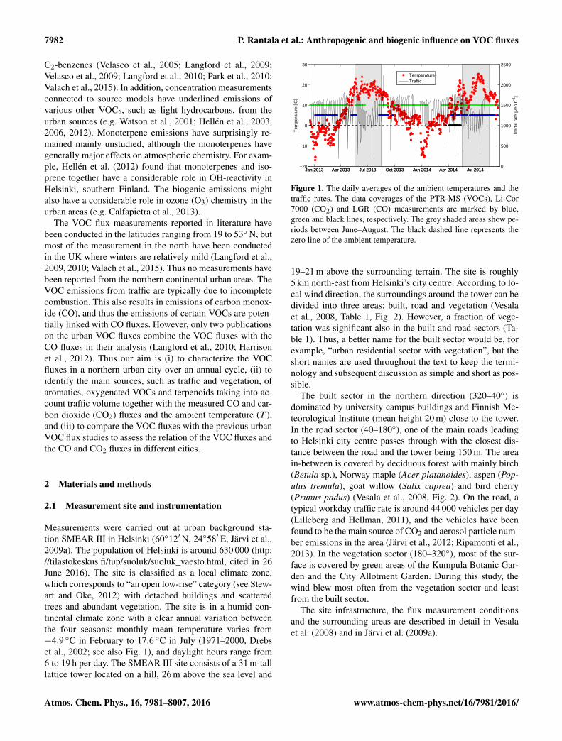
Figure 1. The daily averages of the ambient temperatures and thetraffic rates. The data coverages of the PTR-MS (VOCs), Li-Cor7000 (CO2) and LGR (CO) measurements are marked by blue,green and black lines, respectively. The grey shaded areas show pe-riods between June–August. The black dashed line represents thezero line of the ambient temperature.
19–21 m above the surrounding terrain. The site is roughly5 km north-east from Helsinki’s city centre. According to lo-cal wind direction, the surroundings around the tower can bedivided into three areas: built, road and vegetation (Vesalaet al., 2008, Table 1, Fig. 2). However, a fraction of vege-tation was significant also in the built and road sectors (Ta-ble 1). Thus, a better name for the built sector would be, forexample, “urban residential sector with vegetation”, but theshort names are used throughout the text to keep the termi-nology and subsequent discussion as simple and short as pos-sible.
The built sector in the northern direction (320–40◦) isdominated by university campus buildings and Finnish Me-teorological Institute (mean height 20 m) close to the tower.In the road sector (40–180◦), one of the main roads leadingto Helsinki city centre passes through with the closest dis-tance between the road and the tower being 150 m. The areain-between is covered by deciduous forest with mainly birch(Betula sp.), Norway maple (Acer platanoides), aspen (Pop-ulus tremula), goat willow (Salix caprea) and bird cherry(Prunus padus) (Vesala et al., 2008, Fig. 2). On the road, atypical workday traffic rate is around 44 000 vehicles per day(Lilleberg and Hellman, 2011), and the vehicles have beenfound to be the main source of CO2 and aerosol particle num-ber emissions in the area (Järvi et al., 2012; Ripamonti et al.,2013). In the vegetation sector (180–320◦), most of the sur-face is covered by green areas of the Kumpula Botanic Gar-den and the City Allotment Garden. During this study, thewind blew most often from the vegetation sector and leastfrom the built sector.
The site infrastructure, the flux measurement conditionsand the surrounding areas are described in detail in Vesalaet al. (2008) and in Järvi et al. (2009a).
Atmos. Chem. Phys., 16, 7981–8007, 2016 www.atmos-chem-phys.net/16/7981/2016/

P. Rantala et al.: Anthropogenic and biogenic influence on VOC fluxes 7983
Table 1. The table presents three sectors around the measurement site and the fraction of vegetation of each sector (fX, see Järvi et al., 2014).The average CO2 flux values (in carbon basis) were taken from Järvi et al. (2012).
fpaved fbuilt fveg Annual CO2 emissions[gC m−2] (five-year average)
All 0.36 0.15 0.49 1760Built (320–40◦) 0.42 0.20 0.38Road (40–180◦) 0.39 0.15 0.46 3500Vegetation (180–320◦) 0.30 0.11 0.59 870
Built
Road
Vegetation
Figure 2. The aerial photograph of the SMEAR III station (©
Kaupunkimittausosasto, Helsinki, 2011). The measurement tower ismarked with a black cross. The white dashed lines represent differ-ent sectors (built, vegetation, road). The turquoise solid line showsborders of cumulative 80 % flux footprint (Kormann and Meixner,2001).
2.1.1 VOC measurements with PTR-MS and volumemixing ratio calculations
A proton-transfer-reaction quadrupole mass spectrometer(PTR-MS, Ionicon Analytik GmbH, Innsbruck, Austria;Lindinger et al., 1998) was measuring 12 different mass-to-charge ratios (m/z, see Table 2) every second hour us-ing a 0.5 s sampling time between 1 January 2013 and27 June 2014. The total sampling cycle was around 7 s(Fig. 1). For the rest of the time the PTR-MS sampled awider range of mass-to-charge ratios but those measurementsare not considered in this study. In addition, we had a shortcampaign between 27 June and 30 September 2014 when 14mass-to-charge ratios were measured using the same 0.5 ssampling time. During the campaign, the two additionalmass-to-charge ratios were m/z 89 and m/z 103. In that pe-riod, the measurement cycle always took 2 h so that m/z 31–
69 were measured during the first andm/z 79–137 during thesecond hour, and the total sampling cycle was around 4.5 s.In summer 2014, there were some data gaps due to softwareproblems (Table 2).
The PTR-MS was located inside a measurement containerand sample air was drawn to the instrument using a PTFEtubing with 8 mm inner diameter (i.d.). The sample line was40 m-long and it was heated (10 W m−1) to avoid conden-sation of water vapour. A continuous air-flow was main-tained in the tube with some variations in the flow rate:first 20 L min−1 (whole year 2013), then 40 L min−1 (un-til 30 May 2014) and then 20 L min−1 (until the end of themeasurements) again. The corresponding Reynolds numberswere around 3500 and 7000 for the lower and higher sampleline flows, respectively. From the main inlet, a side flow of50–100 mL min−1 was drawn to PTR-MS via a 0.5 m-longPTFE tube with 1.6 mm i.d.
The PTR-MS was maintained at a drift tube pressure of2.0–2.2 mbar and primary ion (H3O+) count rate of about10–30×106 counts per second (cps, measured at m/z 21).With these settings, E/N -ratio where E is the electric fieldandN the number density of the gas in the drift tube, was typ-ically around 135 Td (Td= 10−21 V m2). Oxygen level O+2was mostly below 2 % of the H3O+ signal.
The instrument was calibrated every second or third weekusing a diluted VOC standard (Apel-Riemer, accuracy± 5 %;Table 2). The volume mixing ratios were calculated usinga procedure described in detail in Taipale et al. (2008). Be-fore the calibration, SEM voltage (MasCom MC-217) of thePTR-MS was always optimized to get a high enough primaryion signal level (e.g. Kajos et al., 2015). The optimized SEMvoltage was also used in the measurements until the next cal-ibration. The instrumental background was determined everysecond hour by sampling VOC free air, produced with a zeroair generator (Parker Balzon HPZA-3500-220). The intakefor the zero air generator was outside of the measurementcabin close to the ground; thus, the relative humidity wasthe same for both the zero air measurements and the ambi-ent measurements. During the measurement period, the zeroair generator was working sometimes improperly, leading tocontaminated m/z 93 signal. These periods were removedfrom the zero air measurements and replaced by the near-est reliable values. In addition, due to software problems, the
www.atmos-chem-phys.net/16/7981/2016/ Atmos. Chem. Phys., 16, 7981–8007, 2016

7984 P. Rantala et al.: Anthropogenic and biogenic influence on VOC fluxes
Table 2. The list of compounds for which the fluxes were determined for. The compound names and the formulas listed below in thirdand fourth column, respectively, are estimates for the measured mass-to-charge ratios (see e.g. de Gouw and Warneke, 2007). The secondcolumn shows whether a sensitivity was determined directly from the calibration or from a transmission curve (i.e. calculated), and whichcompounds were used in the calibrations. LoD shows the average limit of detection for 0.5 s measurement (1.96σ ). Note that m/z 89 andm/z 103 were measured only during 27 June–27 August 2014. Due to software problems, some data were lost. Those gaps are marked bysuperscripts a and b that correspond to the lost periods between 27 June–9 July 2014 and between 27 August–30 September, respectively.The second final column shows the flux data coverages for each of the compound from the whole period January 2013–September 2014.
(m/z) Calibration compound Compound Chemical formula Data coverage (%) LoD (ppt)
31a calculated formaldehyde CH2O – –33a methanol methanol CH4O 32.2 39742a acetonitrile acetonitrile, alkane products C2H3N 32.4 3545a acetaldehyde acetaldehyde C2H4O 32.6 14147a calculated ethanol, formic acid C2H6O, CH2O2 32.9 –59a acetone acetone, propanol C3H6O 37.0 7169a isoprene isoprene, furan, cycloalkanes C5H8 32.1 10579b benzene benzene C6H6 32.8 6081b α-pinene monoterpene fragments 28.5 12089b calculated unknown – – –93b toluene toluene C7H8 31.7 295
103b calculated unknown – – –107b m-xylene,o-xylene C2–benzenes C8H10 30.9 197137b α-pinene monoterpenes C10H16 – –
zero air measurements were not recorded between 7 July and30 September 2014. These gaps were replaced by a mediandiurnal cycle values of the zero air measured during 27 June–7 July 2014. One should note that the mentioned problemswith the zero air measurements had no effect on the fluxcalculations. However, they did, of course, cause additionaluncertainties in the measured concentration levels but a sys-tematic error for the concentration levels was estimated to benegligible.
2.1.2 Ancillary measurements and data processing
An ultrasonic anemometer (Metek USA-1, Metek GmbH,Germany) was installed at 31 m, 0.13 m above the VOC sam-pling inlet. The ambient temperature was also measured atthe VOC sampling level with a Pt-100 sensor. Photosyntheticphoton flux density was measured at 31 m in the measure-ment tower using a photodiode sensor (Kipp & Zonen, Delft,Netherlands). Pressure was measured with Vaisala HMP243barometer on the roof of the University building near the site.
Hourly traffic rates were measured 4 km from the measure-ment site by the City of Helsinki Planning Department. Theserates were converted to correspond to the traffic rates of theroad next to the measurement site following the procedurepresented in Järvi et al. (2012).
CO2 and CO concentrations (10 Hz) were measured witha Li-Cor 7000 (LI-COR, Lincoln, Nebraska, USA) and aCO/N2O analyser (Los Gatos Research, model N2O/CO-23d, Mountain View, CA, USA; later referred as LGR),respectively. The CO2 concentration was measured contin-
uously between January 2013 and September 2014. TheCO concentration was measured between 3 April and27 May 2014 (Fig. 1) and the LGR was connected to thesame main inlet line with the PTR-MS. During the CO mea-surements, the main inlet flow was 40 L min−1. After theLGR was removed from the setup, the main inlet flow wasdecreased to 20 L min−1 to increase the pressure in the sam-pling tube and to get a higher side flow to the PTR-MS (from50 to 100 mL min−1).
Thirty-minute-average CO and CO2 fluxes were calculatedusing the eddy covariance technique from raw data accordingto commonly accepted procedures (Aubinet et al., 2012). Atwo-dimensional (2-D) coordinate rotation was applied to thewind data and all data were linearly de-trended. The 2-D ro-tation was used instead of a planar fitting as the 2-D rotationis likely to be less prone to systematic errors above a com-plex urban terrain (Nordbo et al., 2012b). Spike removal wasmade based on a difference limit (Mammarella et al., 2016).Time lags between wind and scalar data were obtained bymaximizing the cross-covariance function. For the CO andCO2 measurements, mean time lags of 5.8 and 7.0 s, respec-tively, were obtained. Finally, spectral corrections were ap-plied. The low frequency losses for the fluxes were correctedbased on theoretical corrections (Rannik and Vesala, 1999),whereas the high-frequency losses were experimentally de-termined. Finally, the 30 min fluxes were quality checked forstationarity with a limit of 0.3 (Foken and Wichura, 1996),and the periods with u∗ < 0.2 m s−1 were removed from fur-ther analysis. More details of the data post-processing can befound in Nordbo et al. (2012b). The corresponding data cov-
Atmos. Chem. Phys., 16, 7981–8007, 2016 www.atmos-chem-phys.net/16/7981/2016/

P. Rantala et al.: Anthropogenic and biogenic influence on VOC fluxes 7985
erages for CO and CO2 fluxes were 54.0 and 61.9 %, respec-tively. The random error and detection limit of CO flux were0.23 µg m−2 s−1 and 0.16 µg m−2 s−1, respectively. The cor-responding numbers for the CO2 flux were 0.05 µg m−2 s−1
and 0.03 µg m−2 s−1, respectively.
2.2 VOC flux calculations
2.2.1 Disjunct eddy covariance method
In a disjunct eddy covariance method (hereafter DEC), theflux is calculated using a discretized covariance:
w′c′ ≈1n
n∑i=1
w′(i− λ/1t)c′(i), (1)
where n is the number of measurements during the flux av-eraging time, 1t is a sampling interval and λ is a lag timecaused by sampling tubes (e.g. Rinne et al., 2001; Karl et al.,2002; Rinne and Ammann, 2012). The VOC fluxes were cal-culated for each 45 min period according to Eq. (1) using 385data points (600 data points between 26 June and 30 Septem-ber 2016). Before the calculations, the linear trend was re-moved from the concentration and wind measurements. Inaddition, the 2-D rotation was applied to the wind vectors.
The PTR-MS and the wind data were recorded to sepa-rate computers; thus, lag times were shifting artificially as thecomputer clocks performed unequally. Therefore, we first de-termined lag times ofm/z 37 (first water cluster, H3O+H2O)for each data set between two calibrations. Then, a lineartrend was removed from the lag times to cancel the artificialshift. After that, the shifted cross covariance functions weresummed (as in Park et al., 2013), and an average lag-time wasdetermined for each mass-to-charge ratio from the summedcross covariance functions. Finally, the lag-time for each45 min period was determined by using a ±2.5 s lag timewindow around the previously determined mean lag-timewith a smoothed maximum covariance method described inTaipale et al. (2010). The smoothed cross covariance func-tions were calculated using a running mean with an averag-ing period of ±2.4 s. However, if the mean lag-time valuewas not found, the previous reliable mean lag-time value wasused instead. We defined that the mean lag-time was rep-resentative if a peak value of the summed cross covariancefunction was higher than 3σtail where σtail is mean standarddeviation of the summed cross covariance function tails. Thestandard deviations were calculated using a lag-time windowof±(180–200) s. If a certain mass-to-charge ratio showed norepresentative peak values during the whole period at all, itsflux values were defined to be insignificant and the mass-to-charge ratio was disregarded from further study.
The lag times were allowed to vary slightly (±2.5 s)around the mean lag-times because removing the linear trendpotentially caused uncertainties. Moreover, changes in rela-tive humidity might have led to changes in the lag times at
least in the case of methanol which is a water-soluble com-pound, even with heated inlet line. Thus, the fluxes couldbe underestimated if the constant lag-times were used (seesupplementary material). However, the lag time window weused, was quite narrow, ±2.5 s, to limit uncertainties (“mir-roring effect”) caused by the maximum covariance methodconnected to the fluxes near the detection limit (Langfordet al., 2015). Also, one should note that in our case the max-imum covariance was determined from the smoothed crosscovariance function which already limits the possible over-estimation of the measured DEC fluxes, and thus the mirror-ing effect (Taipale et al., 2010). Some flux values could beslightly underestimated if the correct lag-time was outsideof the ±2.5 s window. Figure S1 in the Supplement shows acomparison of the fluxes that were calculated using a con-stant lag-time and the fluxes obtained in this study.
The fluxes measured by the DEC method suffer from samesources of systematic underestimation as the fluxes measuredby the EC method, including the high and low frequencylosses (e.g. Moore, 1986; Horst, 1997). According to Horst(1997), the high frequency losses, αhorst, can be estimatedusing an equation
(αhorst)−1=
11+ (2πfmτ)β
, (2)
where τ is the response time of the system, fm = nmu/(zm−d) and β = 7/8 and β = 1 in unstable and stable stratifica-tion, respectively. In here, u is the mean horizontal wind, zmis the measurement height and d corresponds to the zero dis-placement height. The parameter nm has been observed to beconstant in the unstable stratification at the site (nm = 0.1),and in the stable stratification (ζ > 0) having the followingexperimental, stability and wind direction dependent values(Järvi et al., 2009b):
nm =
0.1(1+ 2.54ζ 0.28), d = 13 m, (built)
0.1(1+ 0.96ζ 0.02), d = 8 m, (road)0.1(1+ 2.00ζ 0.27), d = 6 m, (vegetation),
(3)
where ζ is the stability parameter.A constant response time of 1.0 s and Eq. (2) were used for
the high-frequency flux corrections. The constant value wasestimated based on the previous studies with PTR-MS (Am-mann et al., 2006; Rantala et al., 2014; Schallhart et al., 2016)where the response time of the measurement setup was esti-mated to be around 1 s. However, the response time is prob-ably compound dependent as methanol might have a depen-dence on the relative humidity (RH) due to its polarity andwater solubility. The response time of water vapour has beenobserved to increase as a function of RH (e.g. Ibrom et al.,2007; Mammarella et al., 2009; Nordbo et al., 2012b) andthis is likely true for methanol as well. In addition, the lengthof the sampling tube affects the response time as well butthe effect is difficult to quantify without experimental data(Nordbo et al., 2013).
www.atmos-chem-phys.net/16/7981/2016/ Atmos. Chem. Phys., 16, 7981–8007, 2016
7986 P. Rantala et al.: Anthropogenic and biogenic influence on VOC fluxes
The correction factor αhorst for the high frequency losseswas 1.16 on average. Even though the use of the constantvalue of τ = 1.0 s may lead to random uncertainties if thetrue response time varies temporally, this is likely to onlyhave a small effect on the calculated fluxes. Also a system-atic error of few percentage points is possible, if the actualaverage response time was smaller or higher. We can alsonote that the change of the flow rate from 20 to 40 L min−1
had only a negligible effect on the attenuation as long as theflow is turbulent (see Nordbo et al., 2014).
In addition to the high frequency losses and lag-timesearching routines, the calculated flux values may also bebiased by some other factors. For short-lived isoprene andmonoterpenes (minimum lifetimes ca. 2 h, see Hellén et al.,2012), the flux losses due to chemical degradation were esti-mated to be few percentages (see Rinne et al., 2012). How-ever, these losses are difficult to compensate as they do de-pend on oxidant concentrations (mainly OH and O3) andon surface layer mixing. Thus, no corrections due to thechemical degradation were applied. All the flux values wereslightly underestimated (< 3 % based on the measured CO2fluxes) as the low frequency corrections were left out due tonoisy VOC spectra. Larger errors might be produced by cali-bration uncertainties that directly affect the measured fluxes.All mass-to-charge ratios excludingm/z 47 (ethanol+formicacid) were directly calibrated against a standard in this study.According to Kajos et al. (2015), the concentrations of thecalibrated compounds may also be biased. The flux valuesof ethanol+formic acid should be considered with particu-lar caution as the concentrations of m/z 47 signal was scaledbased on transmission curves (see Taipale et al., 2008).
Periods when the anemometer or the PTR-MS were work-ing improperly, were removed from the time series (Fig. 1).For example, the fluxes were not measured during summer2013 due to a thunderstorm that broke the anemometer, andin the beginning of 2014, when the PTR-MS was serviced.During some periods, signal levels did not behave normallybut had for example a lot of spikes. Those periods were dis-regarded as well. To limit the underestimation of the abso-lute flux values caused by weak mixing, the fluxes duringwhich u∗ < 0.2 m s−1 were rejected from further analysis.Other quality controls, such as filtering the flux data withthe flux detection limits or with the stationarity criteria (Fo-ken and Wichura, 1996), was not performed because apply-ing these methods for the noisy DEC data would potentiallybring other uncertainty sources. For example, disregardingthe fluxes below the detection limit would lead to an overes-timation of the mean absolute flux values. However, beforecalculating correlation coefficients between a specific VOCand another compound (CO, CO2 or another VOC), a per-centage (1 %) of the lowest and highest values were removedto avoid effect of possible outliers. Data coverages for VOCfluxes are listed in Table 2.
2.2.2 Identification of measured mass-to-charge ratios
Identifications of the measured mass-to-charge ratios arelisted in Table 2. Most of the identifications are clear butthere are some exceptions. First of all, p-cymene fragmentsto the same m/z 93 as toluene (Tani et al., 2003); therefore,p-cymene may potentially have an influence on the observedconcentrations at m/z 93 as the used E/N -ratio, 135 Td, cancause fragmentation of p-cymene (Tani et al., 2003). How-ever, Hellén et al. (2012) observed that the p-cymene con-centrations at the SMEAR III site are low compared with thetoluene concentrations, being around 9 % in July. Therefore,the major compound at m/z 93 was likely toluene, althoughp-cymene might have increased the fluxes at m/z 93 duringwarm days.
Anthropogenic furan (de Gouw and Warneke, 2007) andcycloalkanes probably constituted a major contribution to themeasured m/z 69 concentrations between October and Mayas isoprene concentrations at the site are reported to be small(around 5–30 ppt; Hellén et al., 2006, 2012). In our study,the mean m/z 69 concentrations between June and Augustwere only ca. 60 % larger than during the other seasons (Ta-ble 3), indicating a considerable influence of furan and cy-cloalkanes (e.g. cyclohexane, see Hellén et al., 2006 and Leeet al., 2006). Another important compound influencing themeasurements at m/z 69 is methylbutenol (MBO) fragment(e.g. Karl et al., 2012). However, MBO is mostly emittedby conifers (e.g. Guenther et al., 2012) that are rare nearthe SMEAR III station. Therefore, MBO should only havea negligible effect on the concentration and fluxes measuredat m/z 69.
Monoterpenes fragment to them/z 81. The parental mass-to-charge ratio of the monoterpenes, m/z 137, had a lowsensitivity during the study, and therefore, the monoter-pene concentrations were calculated using m/z 81. For somereason the monoterpene concentrations were only slightlyhigher during the summer than during the other seasons (Ta-ble 3). Therefore, a contribution of other compounds thanmonoterpenes at m/z 81 can be possible. On the other hand,Hellén et al. (2012) observed also considerable monoterpeneconcentrations at the site in winter, spring and fall, possiblydue to anthropogenic sources.
Acetone and propanal are both measured at m/z 59 withthe PTR-MS but Hellén et al. (2006) showed that the aver-age propanal concentrations were only around 5 % comparedwith the average acetone concentrations in Helsinki duringwinter. Thus, most of the m/z 59 signal consisted probablyof acetone. However, as propanal fluxes at the site are un-known, m/z 59 will still be referred as acetone+propanal.
Measurements at m/z 107 consisted of C2-benzenes in-cluding, for example, o- and p+m-xylene and ethylbenzene.According to Hellén et al. (2012), major compounds mea-sured at the site is p+m-xylene. Other important compoundsreported are o-xylene and ethylbenzene. Hellén et al. (2012)observed annual variation for those compounds with a mini-
Atmos. Chem. Phys., 16, 7981–8007, 2016 www.atmos-chem-phys.net/16/7981/2016/
P. Rantala et al.: Anthropogenic and biogenic influence on VOC fluxes 7987
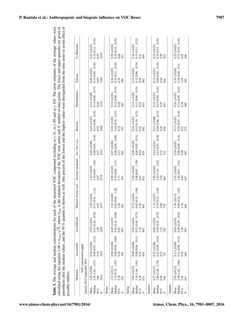
Tabl
e3.
The
aver
age
and
med
ian
conc
entr
atio
nsfo
rea
chof
the
mea
sure
dV
OC
com
poun
dex
clud
ingm/z
31,m/z
89an
dm/z
103.
The
erro
res
timat
esof
the
aver
age
valu
esw
ere
calc
ulat
edus
ing
the
equa
tion
1.96×σ
voc/√N
,whe
reσ
voc
isth
est
anda
rdde
viat
ion
ofth
eV
OC
time
seri
esan
dN
num
ber
ofda
tapo
ints
.The
low
eran
dup
per
quar
tiles
are
give
nin
pare
nthe
sis
afte
rth
em
edia
nva
lues
,and
the
95%
quan
tile
issh
own
asw
ell.
One
perc
ento
fth
elo
wes
tand
the
high
estv
alue
sw
ere
disr
egar
ded
from
the
time
seri
esto
avoi
def
fect
ofpo
ssib
leou
tlier
s.
Met
hano
lA
ceto
nitr
ileA
ceta
ldeh
yde
Eth
anol+
form
icac
idA
ceto
ne+
prop
anal
iso.+
fur.+
cyc.
Ben
zene
Mon
oter
pene
sTo
luen
eC
2-B
enze
nes
VO
Cco
ncen
trat
ion
[ppb
]Ja
nuar
y20
13–S
epte
mbe
r201
4
Mea
n3.
28(±
0.09
)0.
10(±
0.00
)0.
59(±
0.01
)1.
05(±
0.04
)1.
45(±
0.03
)0.
10(±
0.00
)0.
19(±
0.01
)0.
14(±
0.00
)0.
20(±
0.01
)0.
22(±
0.01
)M
edia
n2.
58(1
.61...
4.57
)0.
09(0
.07...
0.13
)0.
51(0
.36...
0.76
)0.
71(0
.41...
1.22
)1.
30(0
.85...
1.89
)0.
08(0
.05...
0.14
)0.
13(0
.08...
0.25
)0.
12(0
.08...
0.17
)0.
14(0
.05...
0.28
)0.
18(0
.12...
0.29
)95
%7.
660.
191.
204.
072.
970.
270.
520.
280.
630.
52N
2415
2431
2451
2477
2779
2412
2462
2139
2383
2319
Win
ter
Mea
n1.
33(±
0.11
)0.
06(±
0.00
)0.
49(±
0.03
)1.
01(±
0.08
)0.
89(±
0.05
)0.
07(±
0.00
)0.
45(±
0.02
)0.
13(±
0.01
)0.
36(±
0.02
)0.
30(±
0.02
)M
edia
n1.
13(0
.79...
1.67
)0.
06(0
.05...
0.08
)0.
43(0
.34...
0.60
)0.
82(0
.60...
1.26
)0.
79(0
.60...
1.11
)0.
06(0
.04...
0.08
)0.
44(0
.34...
0.57
)0.
12(0
.09...
0.15
)0.
32(0
.21...
0.45
)0.
26(0
.18...
0.38
)95
%2.
780.
100.
912.
261.
710.
130.
720.
290.
700.
66N
176
199
207
203
354
203
357
203
380
371
Spri
ng
Mea
n3.
05(±
0.15
)0.
09(±
0.00
)0.
59(±
0.02
)0.
75(±
0.04
)1.
28(±
0.04
)0.
09(±
0.00
)0.
18(±
0.01
)0.
12(±
0.00
)0.
15(±
0.01
)0.
18(±
0.01
)M
edia
n2.
18(1
.46...
3.81
)0.
08(0
.06...
0.11
)0.
53(0
.40...
0.73
)0.
65(0
.35...
1.00
)1.
08(0
.83...
1.58
)0.
08(0
.05...
0.11
)0.
15(0
.10...
0.23
)0.
11(0
.08...
0.15
)0.
12(0
.06...
0.19
)0.
15(0
.11...
0.22
)95
%8.
200.
151.
101.
922.
610.
190.
410.
220.
450.
41N
874
876
905
891
915
879
892
853
892
859
Sum
mer
Mea
n4.
27(±
0.17
)0.
12(±
0.00
)0.
60(±
0.02
)1.
15(±
0.07
)1.
88(±
0.05
)0.
14(±
0.01
)0.
11(±
0.00
)0.
15(±
0.01
)0.
12(±
0.01
)0.
23(±
0.01
)M
edia
n3.
88(2
.40...
5.70
)0.
12(0
.09...
0.15
)0.
50(0
.35...
0.79
)0.
79(0
.52...
1.40
)1.
70(1
.24...
2.42
)0.
12(0
.07...
0.18
)0.
09(0
.06...
0.14
)0.
13(0
.09...
0.18
)0.
08(0
.02...
0.18
)0.
19(0
.13...
0.29
)95
%8.
560.
211.
224.
003.
540.
320.
260.
290.
440.
50N
748
751
756
778
863
743
938
823
826
823
Aut
umn
Mea
n2.
95(±
0.13
)0.
11(±
0.00
)0.
62(±
0.03
)1.
36(±
0.13
)1.
41(±
0.05
)0.
10(±
0.01
)0.
13(±
0.01
)0.
16(±
0.01
)0.
35(±
0.04
)0.
25(±
0.02
)M
edia
n2.
58(1
.62...
3.96
)0.
11(0
.06...
0.15
)0.
50(0
.29...
0.92
)0.
60(0
.26...
1.65
)1.
46(0
.67...
1.91
)0.
06(0
.04...
0.14
)0.
10(0
.07...
0.16
)0.
14(0
.09...
0.21
)0.
30(0
.08...
0.5)
0.21
(0.1
0...
0.35
)95
%5.
810.
191.
294.
362.
640.
280.
310.
361.
030.
62N
617
605
583
605
647
587
275
260
285
266
www.atmos-chem-phys.net/16/7981/2016/ Atmos. Chem. Phys., 16, 7981–8007, 2016

7988 P. Rantala et al.: Anthropogenic and biogenic influence on VOC fluxes
mum in March. In our study, only small differences betweenthe seasons were observed (Table 3). However, the measuredconcentrations in this study were quite close to the corre-sponding values in Hellén et al. (2012). For example, thesummed concentration of o-, p+m-xylene and ethylbenzenewas ca. 0.16 ppb in July (Hellén et al., 2012) whereas in thisstudy, a mean value from June–August was 0.23 ppb (Ta-ble 3).
The mass-to-charge ratio 42 is connected with acetonitrilebut Dunne et al. (2012) observed that the signal might bepartly contaminated by product ions formed in reactions withNO+ and O+2 that exist as trace amounts inside the PTR-MS.However, this effect was impossible to quantify in this study,and thus,m/z 42 was assumed to consist of acetonitrile. Gen-erally, acetonitrile is used as a marker for biomass burningas it is released from those processes (e.g. Holzinger et al.,1999; De Gouw et al., 2003; Patokoski et al., 2015).
2.3 Estimating biogenic contribution of isoprene
A well-known algorithm for isoprene emissions (Eiso) iswritten as
Eiso = E0,synthCTCL, (4)
where E0,synth, CT and CL are the same as in the traditionalisoprene algorithm (Guenther et al., 1991, 1993; Guenther,1997). The shape of this algorithm is based on the light re-sponse curve of the electron transport activity (CL) and onthe temperature dependence of the protein activity (CT ). Theemission potential, E0,synth, describes the emission rate ofisoprene at T = 30 ◦C where T is the leaf temperature (theambient temperature in this study).
The algorithm was used to identify possible biogenic iso-prene emissions. For other compounds, such as methanol ormonoterpenes, no empirical algorithms were applied.
3 Results and discussion
3.1 Seasonal behaviour of observed fluxes andconcentrations
Significant fluxes were observed for methanol (m/z 33),acetaldehyde (m/z 45), ethanol+formic acid (m/z 47),acetone+propanal (m/z 59), isoprene+furan+cycloalkanes(m/z 69, later referred as iso.+fur.+cyc.), benzene (m/z 79),toluene (m/z 93), C2-benzenes (m/z 107) and sum ofmonoterpenes (m/z 81). The fluxes of these compounds alsohad a diurnal cycle at least in one of the wind sectors (Fig. 3,Table 1). Correlation coefficients between VOC, CO, CO2fluxes and traffic rates are shown in Table A1 in the Supple-ment.
Methyl tert-butyl ether (MTBE) and tert-Amyl methylether (TAME) are commonly connected to the vehi-cle exhaust emissions as the compounds were at least
used to increase the octane number of gasoline (e.g.Hellén et al., 2006). MTBE and TAME were measured attheir parental ions atm/z 89 andm/z 103, respectively. How-ever, both mass-to-charge ratios showed no significant fluxes,and therefore, those measurements were excluded from fur-ther analysis. As the identification of these mass-to-chargeratios was uncertain, both m/z 89 and m/z 103 are markedas unknown in Table 2. Formaldehyde, which was measuredat m/z 31 showed no fluxes either. Therefore, m/z 31 wasexcluded from further analysis as well.
All of the studied compounds except acetonitrile hadsignificant fluxes during winter (Table 4), indicating an-thropogenic sources. All compounds except acetonitrile,iso.+fur.+cyc. and monoterpenes also had a significant dif-ference between weekday and weekend values (Fig. 4) whichis also a strong anthropogenic signal as many anthropogenicactivities can expected to be lower during the weekend thanduring the weekdays.
The toluene and C2-benzene fluxes showed statisticallysignificant seasonal variation with a maximum in winterand a minimum in summer–autumn (Table 4 and Fig. 5).However, the variations were rather small because the bio-genic emissions of these compounds should be either smallor negligible, and the anthropogenic emissions are unlikelyto have large seasonal variations. Nevertheless, the trafficcounts were lower during June–August (Fig. 1). The aver-age benzene fluxes had statistically no significant differencesbetween the seasons (Table 4 and Fig. 5). A ratio betweenthe average toluene or C2-benzene and benzene fluxes hadno considerable seasonal trend either (Table A2).
The benzene and toluene concentrations had a clear annualtrend with a minimum during June–August. This is a well un-derstood pattern and it is partly caused by the different atmo-spheric lifetimes of these compounds between seasons (e.g.Hellén et al., 2012). Of course, local sources may affect theobserved concentration trend as well if the boundary layerheight has a seasonal cycle. The concentrations of all aro-matic compounds also had a diurnal cycle with a maximumduring morning rush hours when the traffic-related emissionswere high and the atmospheric boundary layer was still shal-low after the night (Fig. 6). The behaviour is similar com-pared with the CO and CO2 concentrations.
A clear biogenic signal was observed for iso.+fur.+cyc.which had a large difference in both the fluxes and concen-trations between winter and summer (Tables 4–3). There-fore, the fraction of terpenoid to the total VOC fluxes wasalso higher in the summer than in the winter (Fig. 7). Theiso.+fur.+cyc. flux followed also well the ambient temper-ature (Fig. 8). The monoterpene fluxes were significantlyhigher during the summer, but the average flux during thewinter was considerable as well (Table 4), indicating othermajor sources than only the biogenic ones. Interestingly,both the monoterpene and iso.+fur.+cyc. concentrationspeaked during morning rush hour (Fig. 6), indicating an
Atmos. Chem. Phys., 16, 7981–8007, 2016 www.atmos-chem-phys.net/16/7981/2016/

P. Rantala et al.: Anthropogenic and biogenic influence on VOC fluxes 7989
Tabl
e4.
The
aver
age
and
med
ian
fluxe
sfo
rea
chm
easu
red
VO
Cco
mpo
und
excl
udin
gm/z
31,m/z
89an
dm/z
103.
The
erro
res
timat
esof
the
aver
age
valu
esw
ere
calc
ulat
edus
ing
the
equa
tion
1.96·σ
voc/√N
,whe
reσ
voc
isth
est
anda
rdde
viat
ion
ofth
eV
OC
time
seri
esan
dN
num
ber
ofda
tapo
ints
.The
low
eran
dup
per
quar
tiles
are
give
nin
pare
nthe
sis
afte
rth
em
edia
nva
lues
.One
perc
ento
fth
elo
wes
tand
the
high
estv
alue
sw
ere
disr
egar
ded
from
the
time
seri
esto
avoi
def
fect
ofpo
ssib
leou
tlier
s.T
hem
ean
dete
ctio
nlim
its(L
oD)
wer
eca
lcul
ated
asL
oD=
1/N
∑ LoD
2 i(V
alac
het
al.,
2015
)w
here
sing
lede
tect
ion
limits
,LoD
,wer
ede
fined
tobe
1.96σ
ccf
whe
reσ
ccf
isth
est
anda
rdde
viat
ion
ofcr
oss
cova
rian
ceta
ils(T
aipa
leet
al.,
2010
).T
heac
eton
itrile
flux
was
belo
wL
oDin
the
win
ter.
Met
hano
lA
ceto
nitr
ileA
ceta
ldeh
yde
Eth
anol+
form
icac
idA
ceto
ne+
prop
anal
iso.+
fur.+
cyc.
Ben
zene
Mon
oter
pene
sTo
luen
eC
2-B
enze
nes
VO
Cflu
x[n
gm−
2s−
1 ]Ja
nuar
y20
13–S
epte
mbe
r201
4
Mea
n44
.9(±
2.5)
0.7
(±0.
1)10
.1(±
0.6)
21.9
(±1.
7)16
.7(±
1.1)
8.0
(±0.
6)5.
5(±
0.6)
10.9
(±1.
2)14
.1(±
1.1)
16.4
(±1.
4)M
edia
n29
.4(1
0.4...
62.2
)0.
7(−
1.2...
2.2)
8.3
(2.4...1
6.7)
16.5
(−0.
8...
35.2
)11
.6(2
.1...2
5.9)
5.5
(−0.
7...
14)
4.6
(−2.
2...
11.2
)11
.0(−
5.7...
25.6
)11
.4(−
1.3...
26)
14.6
(−3.
7...
33.0
)L
oD1.
20.
10.
51.
00.
70.
30.
50.
90.
71.
0N
2021
2034
2050
2066
2311
2018
2090
1820
2029
1983
Win
ter
Mea
n35
.5(±
7.9)
–5.
0(±
1.3)
46.4
(±8.
8)17
.4(±
3)2.
4(±
1.4)
7.3
(±2.
3)8.
5(±
3.4)
19.6
(±3.
1)24
.6(±
4.0)
Med
ian
16.4
(4.8...4
2.4)
–5.
1(−
0.6...
9.7)
26.7
(8.2...6
9.9)
11.6
(3.0...2
7)2.
4(−
1.9...
5.7)
5.9
(−6.
3...
20.6
)8.
1(−
4.5...
19.7
)15
.5(1
.3...3
5.2)
23.3
(0.9...4
3.8)
LoD
3.0
0.3
1.3
4.0
2.5
1.0
2.2
3.5
2.5
3.5
N17
8–
185
179
327
182
315
181
328
324
Spri
ng
Mea
n52
.1(±
4.7)
0.9
(±0.
2)10
.7(±
1.1)
26.2
(±3.
3)16
.4(±
1.8)
4.9
(±0.
8)5.
7(±
1.0)
8.9
(±2.
0)13
.9(±
1.9)
16.5
(±2.
4)M
edia
n31
.8(1
0.6...
75.5
)0.
8(−
1.3...
2.5)
8.3
(1.7...1
8.6)
18.4
(−2.
2...
43)
11.2
(1.1...2
5.9)
3.8
(−2.
6...
11.3
)5.
0(−
2.7...
12.2
)8.
4(−
11.5...2
6.4)
11.7
(−4.
0...
27.3
)15
.2(−
5.4...
33.7
)L
oD2.
30.
21.
12.
01.
30.
60.
81.
61.
11.
7N
758
765
775
765
789
762
775
731
778
755
Sum
mer
Mea
n54
.2(±
4.5)
0.6
(±0.
2)11
.8(±
1.0)
14.7
(±2.
2)20
.6(±
2.1)
14.3
(±1.
4)4.
8(±
0.8)
14.1
(±1.
8)13
.2(±
1.5)
14.0
(±1.
9)M
edia
n39
.1(1
5.7...
76.0
)0.
8(−
1.1...
2.0)
9.4
(3.9...1
8.1)
14.1
(−2.
4...
29.3
)15
.0(4
.4...3
0.2)
9.1
(2.1...2
2.6)
4.0
(−1.
1...
9.3)
12.8
(0.4...2
6.1)
10.8
(2.6...2
2.0)
13.1
(−2.
4...
29.4
)L
oD2.
30.
10.
61.
21.
20.
70.
51.
40.
91.
5N
623
622
626
643
710
608
782
689
688
688
Aut
umn
Mea
n24
.4(±
2.5)
0.7
(±0.
3)9.
0(±
1.0)
15.6
(±2.
5)10
.8(±
2.1)
7.3
(±1.
0)4.
1(±
1.2)
9.3
(±3.
0)10
.0(±
3.6)
11.2
(±3.
5)M
edia
n21
.4(6
.3...4
2.6)
0.7
(−1.
1...
2.2)
8.4
(2.7...1
4.3)
14.6
(−1.
5...
31.2
)7.
4(−
1.2...
17.9
)5.
8(−
0.1...
12.6
)4.
1(−
1.4...
8.5)
9.6
(−6.
0...
25.8
)7.
0(−
6.6...
22.0
)8.
5(−
7.3...
26.9
)L
oD1.
80.
10.
41.
20.
90.
40.
71.
83.
02.
0N
462
465
464
479
485
466
218
219
235
216
www.atmos-chem-phys.net/16/7981/2016/ Atmos. Chem. Phys., 16, 7981–8007, 2016

7990 P. Rantala et al.: Anthropogenic and biogenic influence on VOC fluxes
RoadVegetationBuilt
Figure 3. The median diurnal VOC fluxes from the three sectors for each of the compound (January 2013–September 2014). The blue circles,red crosses and black crosses correspond to the road sector, the vegetation sector and the built sector, respectively. The vertical lines showthe lower and upper quartiles (25 and 75 %). Due to scaling, one upper quartile value is not shown in the acetone+propanal figure.
Table 5. The statistics of the measured CO and CO2 fluxes and the CO concentrations from each wind sector (3 April–27 May 2014). Theerror estimates of the average values were calculated using the equation 1.96 · σ/
√N , where σ is the standard deviation of the CO or CO2
time series and N the number of data points. The lower and upper quartiles are given in parenthesis after the median values.
All Built Road Vegetation
CO flux [µg m−2 s−1]Mean 0.69± 0.05 0.57± 0.11 1.46± 0.15 0.35± 0.03Median 0.36 (0.11–0.86) 0.37 (0.22–0.75) 1.18 (0.54–2.08) 0.26 (0.10–0.48)
CO2 flux [µg m−2 s−1]Mean 138± 9 157± 34 282± 27 71± 9Median 111 (57–198) 123 (68–177) 257 (135–378) 80 (31–123)
CO concentration [ppb]Mean 146.5± 1.0 152.7± 5.6 152.6± 1.9 143.1± 1.1Median 142.0 (133.8–155.9) 141.2 (132.8–164.4) 148.2 (138.7–161.4) 139.2 (131.8–151.9)
Atmos. Chem. Phys., 16, 7981–8007, 2016 www.atmos-chem-phys.net/16/7981/2016/

P. Rantala et al.: Anthropogenic and biogenic influence on VOC fluxes 7991
0
10
20
30
40
50
Ave
rage
flux
[ng
m−
2 s−1 ]
Met
hano
l*
Aceta
ldehy
de*
Ethan
ol+fo
rmic
acid*
Aceto
ne+p
ropa
nal*
Iso.+
fur.+
cyc.
Benze
ne*
Mon
oter
pene
s
Toluen
e*
C 2−b
enze
nes*
WeekdaysWeekend
Figure 4. The average fluxes for each of the VOCs (exclud-ing acetonitrile) from Saturday+Sunday and from weekdays (Jan-uary 2013–September 2014). The white and the grey bars show theaverage fluxes during the weekdays and Saturday+Sunday, respec-tively. The asterisks in the x axes show if the differences betweenthe average week and the average weekend fluxes were statisticallysignificant. The uncertainties of the average fluxes were calculatedusing the equation ±1.96σvoc/
√N , where σvoc is the standard de-
viation of a VOC flux time series and N the number of data points.
anthropogenic contribution, most likely from traffic-relatedsources.
Methanol had a higher average flux during spring and sum-mer compared with winter and autumn (Table 4 and Fig. 5).Similarly, an average acetaldehyde flux from summer wasaround 100 % larger compared with the winter value, whichmight indicate a significant biogenic contribution during thesummer. For methanol and acetone, the largest difference be-tween the average fluxes was interestingly between summerand autumn season. This cannot be explained by the biogenicemissions as the autumn values were smaller than the winterones (Table 4 and Fig. 5), but it might be a result of changesin the non-traffic-related anthropogenic activity. On the otherhand, the observed differences can be partly explained bywind directions: in summer, 38 % of the time the wind blewfrom the road sector (40–180◦) whereas in autumn, the cor-responding occurrence was only 24 %.
The methanol, acetone and acetaldehyde (OVOCs) con-centrations also had a seasonal cycle with a maximum insummer. However, those compounds showed no clear diurnalcycles, probably due to high ambient background concentra-tions compared with aromatic or terpenoid compounds (Ta-ble 3 and Fig. 6). The ratio of the measured OVOC fluxes tothe total measured VOC fluxes stayed stable, being 48–61 %depending on the season (Fig. 7).
The diurnal concentration level of acetonitrile stayed al-most constant but the concentrations showed an annual trendwith a maximum in summer (Table 3 and Fig. 5). However,this was probably related to advection from distant sources
(e.g. Patokoski et al., 2015). Generally, the average acetoni-trile fluxes were really small being still above the detectionlimits except in winter (Table 4 and Fig. 5).
Both ethanol+formic acid fluxes and concentrations hadsignificant differences between the seasons. However, asthe ethanol+formic acid was not calibrated, the resultsshould be taken as rough estimates. Nevertheless, the aver-age ethanol+formic acid flux seemed to have a maximum inwinter. Their concentration showed also a weak diurnal trendwith minimum during early morning (Fig. 6).
3.2 VOC, CO and CO2 emissions from differentsources
To investigate the relative contributions different sources, thefluxes were analysed by wind sectors. The data was dividedinto three groups based on the local wind direction corre-sponding to built, road and vegetation dominated areas (Ta-ble 1 and Fig. 2). The measured flux value was defined tobe, for example, from the road sector if less than 30 % of theflux footprint area covered other than the road sector. Thus,the periods when wind blew close to a sector border, wererejected from further analysis. The total rejection rate wasaround 30 %. The footprints were determined according toKormann and Meixner (2001).
The CO flux was observed to have a clear diurnal cycle,and as expected, the highest emissions were detected fromthe road sector (Fig. 9) where the traffic emissions are at theirhighest. The measured CO fluxes from the road sector alsocorrelated very well with both the corresponding CO2 fluxes(r = 0.68, p < 0.001) and with the traffic rates (r = 0.56,p < 0.001, Fig. 10). The average and median CO and CO2fluxes and CO concentrations from 3 April–27 May 2014 arepresented in Table 5. The ratio between the median CO andCO2 fluxes was the lowest during night-time due to respira-tion of CO2 from vegetation (Fig. 9). The highest flux valuesof both CO and CO2 were observed during day-time. How-ever, the rush hour peaks cannot be seen from the flux data.On the other hand, the traffic rates were only slightly higherduring the rush hours compared with the other day-time val-ues.
During the measurement period, the average CO flux fromthe road sector was ca. 0.52 % compared with the corre-sponding CO2 flux (Table 5). On the other hand, CO2 prob-ably already experienced biogenic uptake between April andMay 2014 (Järvi et al., 2012; Fig. 9 and Table 5). There-fore, a better estimate for the flux ratio was taken from Järviet al. (2012) who estimated that the CO2 emission rate fromthe road sector is 264 µg m−2 s−1 (1000 veh h−1)−1 which isbased on wintertime data from 5 years. In our study, the cor-responding CO emission rate from traffic was 0.9 µg m−2 s−1
(1000 veh h−1)−1 which is ca. 0.34 % compared with the cor-responding emission rate of CO2 in mass basis. Järvi et al.(2012) used data from a more narrow wind sector, 40–120◦.However, the average CO fluxes had no considerable differ-
www.atmos-chem-phys.net/16/7981/2016/ Atmos. Chem. Phys., 16, 7981–8007, 2016
7992 P. Rantala et al.: Anthropogenic and biogenic influence on VOC fluxes
FluxFlux Flux
Flux Flux Flux
Flux Flux Flux
FluxFlux
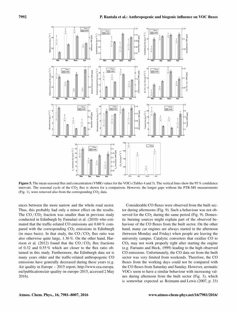
Figure 5. The mean seasonal flux and concentration (VMR) values for the VOCs (Tables 4 and 3). The vertical lines show the 95 % confidenceintervals. The seasonal cycle of the CO2 flux is shown for a comparison. However, the longer gaps without the PTR-MS measurements(Fig. 1), were removed also from the corresponding CO2 data.
ences between the more narrow and the whole road sector.Thus, this probably had only a minor effect on the results.The CO /CO2 fraction was smaller than in previous studyconducted in Edinburgh by Famulari et al. (2010) who esti-mated that the traffic-related CO emissions are 0.60 % com-pared with the corresponding CO2 emissions in Edinburgh(in mass basis). In that study, the CO /CO2 flux ratio wasalso otherwise quite large, 1.36 %. On the other hand, Har-rison et al. (2012) found that the CO /CO2 flux fractionsof 0.32 and 0.55 % which are closer to the flux ratio ob-tained in this study. Furthermore, the Edinburgh data set ismany years older and the traffic-related anthropogenic COemissions have generally decreased during these years (e.g.Air quality in Europe – 2015 report, http://www.eea.europa.eu//publications/air-quality-in-europe-2015, accessed 2 May2016).
Considerable CO fluxes were observed from the built sec-tor during afternoons (Fig. 9). Such a behaviour was not ob-served for the CO2 during the same period (Fig. 9). Domes-tic burning sources might explain part of the observed be-haviour of the CO fluxes from the built sector. On the otherhand, many car engines are always started in the afternoon(between Monday and Friday) when people are leaving theuniversity campus. Catalytic converters that oxidize CO toCO2 may not work properly right after starting the engine(e.g. Farrauto and Heck, 1999) leading to the high observedCO emissions. Unfortunately, the CO data set from the builtsector was very limited from weekends. Therefore, the COfluxes from the working days could not be compared withthe CO fluxes from Saturday and Sunday. However, aromaticVOCs seem to have a similar behaviour with increasing val-ues during afternoon from the built sector (Fig. 3), whichis somewhat expected as Reimann and Lewis (2007, p. 33)
Atmos. Chem. Phys., 16, 7981–8007, 2016 www.atmos-chem-phys.net/16/7981/2016/

P. Rantala et al.: Anthropogenic and biogenic influence on VOC fluxes 7993
Figure 6. The median diurnal VOC, CO and CO2 volume mixing ratios for each compound. The vertical lines show the 95 % confidenceintervals. The VOC and CO2 data is between January 2013 and September 2014. However, times corresponding to the longer gaps in thePTR-MS data (Fig. 1), were removed also from the CO2 data. The CO data is from April–May 2014.
mentions that the VOC-related “cold start emissions” are be-coming more and more important. On the other hand, noneof the aromatic compounds had a positive correlation withthe CO flux, indicating different sources for CO and for thearomatic compounds.
According to a study by Hellén et al. (2006), the trafficis the most important source for the aromatic compoundsin Helsinki with for example wood combusting explainingless than 1 % of the detected benzene concentrations. How-ever, the study by Hellén et al. (2006) was based on thechemical mass balance receptor model with the VOC con-centrations. Thus, the footprint of their study was largerthan in our work which is based on the flux measurements.The major emissions could originate also from the bio-genic sources, at least in the case of isoprene and monoter-penes (Hellén et al., 2012). Therefore, summertime data ofiso.+fur.+cyc., monoterpenes, and also OVOCs (methanol,
acetone+propanal and acetaldehyde) were analysed morecarefully. Conversely,the aromatic compounds were assumedto have no biogenic emissions, although benzenoid com-pounds might also originate from vegetation (Misztal et al.,2015).
In addition to the traffic, other anthropogenic VOC sourcescould potentially include wood combusting and solvent use.Industry is also a source for the VOCs but no industrial ac-tivities were located inside flux footprint areas. However, thesolvent use might be a significant source for many com-pounds, especially in the built sector where the universitybuildings are located.
3.2.1 Traffic-related emissions
Out of the measured compounds, methanol, acetaldehyde,ethanol, acetone, toluene, benzene, and C2-benzenes are in-
www.atmos-chem-phys.net/16/7981/2016/ Atmos. Chem. Phys., 16, 7981–8007, 2016

7994 P. Rantala et al.: Anthropogenic and biogenic influence on VOC fluxes
48 %
43 %
9 %Winter
61 %
28 %
11 %
Spring
59 %
22 %
19 %
Summer
51 %
29 %
19 %
Autumn
OVOCAromaticsTerpenoids
Figure 7. The fractions of the measured OVOC (methanol, ac-etaldehyde, acetone+propanal), aromatic (benzene, toluene, C2-benzenes) and terpenoid (isoprene+furan+cycloalkanes, monoter-penes) fluxes from each season (in mass basis). Ethanol+formicacid was left out from the analysis as its concentrations were notdirectly calibrated.
gredients of gasoline (Watson et al., 2001; Niven, 2005;Caplain et al., 2006; Langford et al., 2009). Therefore, thetraffic is potentially an important anthropogenic source forthese compounds. In addition, many studies have showntraffic-related isoprene emissions (Reimann et al., 2000; Bor-bon et al., 2001; Durana et al., 2006; Hellén et al., 2006,2012). Hellén et al. (2012) also speculated that some of themonoterpene emissions could originate from the traffic. Ofcourse, the ingredients of gasoline probably do have varia-tions between countries. In Finland, a popular 95E10 gaso-line contains a significant amount of ethanol (< 10 %) andmethanol (< 3 %).
In recent VOC flux studies at urban sites, the fluxes ofsome VOCs have correlated with the traffic rates (Langfordet al., 2009, 2010; Park et al., 2010; Valach et al., 2015) butthis does not necessarily imply causality. At SMEAR III, thetraffic has been shown to be the most important source forCO2 from the road sector (Järvi et al., 2012) and the sameseems to hold also for CO (Table 5). Therefore, the influ-ence of the traffic on the VOC emissions was quantified bystudying the measured VOC fluxes from this direction. Thedifference between the average fluxes from the road sectorand the other sectors was statistically significant (95 % confi-dence intervals) for methanol, acetaldehyde, iso.+fur.+cyc.,benzene and C2-benzenes.
All three studied aromatics (benzene, toluene and C2-benzenes) were assumed to have same main source, the traf-fic. Therefore, the aromatic compounds are analysed together
and they are later referred as the aromatic flux. However, es-pecially toluene and C2-benzenes are also released from sol-vents and paint-related chemicals. These non-traffic-relatedsources were studied by comparing the average toluene andC2-benzene flux with the corresponding average benzeneflux, as benzene was assumed to be emitted from the traffic-related sources only. The ratios between the average tolueneand benzene fluxes from the road, vegetation and built sec-tor were around 2.6 ± 0.4, 2.50 ± 0.7 and 3.70 ± 1.9, re-spectively. The ratios indicate that toluene might have alsoevaporative sources. In previous studies, the exhaust emis-sion ratio between toluene and benzene has been determinedto be around 2 – 2.5 (e.g. Karl et al., 2009 and referencestherein) but the ratio depends on catalytical converters etc.(e.g. Rogers et al., 2006). Above an industrialized regionin Mexico City where toluene also had other major sourcesin addition to traffic, Karl et al. (2009) found the ratio tobe around 10–15. In this study, the corresponding ratiosfor benzene/C2-benzenes were 0.32± 0.05, 0.31± 0.09 and0.30 ± 0.17. In earlier studies (e.g. Karl et al., 2009 and ref-erences therein), the exhaust emission ratio for those com-pounds have been observed to be around 0.4. Thus, bothtoluene and C2-benzenes had probably also other than traffic-related emissions in all the sectors. However, the possiblesources for these non-traffic-related emissions remained un-known. In the built sector, the evaporative emissions from theUniversity buildings might explain part of the toluene andC2-benzene flux.
The traffic rates and the aromatic fluxes had a signif-icant correlation (r = 0.38, p < 0.001, measurements be-tween January 2013 and September 2014) from the roadsector. The aromatic fluxes correlated even better with themeasured CO fluxes (r = 0.50, p < 0.001, measurements be-tween April and May 2014). The significant correlation be-tween the aromatic VOC flux and the CO flux indicates acommon source from incomplete combustion. As these bothcorrelated in also with the traffic rates, the traffic is likely tobe the major source for aromatics.
To estimate the total emission of the aromatic compoundsfrom the traffic, the aromatic fluxes were fitted against thetraffic rates. A linear model between the traffic rates andthe CO2 emissions has been suggested, for example, in Järviet al. (2012). On the other hand, Langford et al. (2010) andHelfter et al. (2011) proposed an exponential fit for the VOCand CO2 emissions. Helfter et al. (2011) mention many rea-sons for the exponential relationship, such as an increasedfuel consumption at higher traffic rates. However, Järvi et al.(2012) did not observe the exponential behaviour betweenthe CO2 fluxes and the traffic rates at the site. Therefore, alinear model was also used in this study. Additionally, theexponential relationship was tested but it brought no clearbenefit compared with the linear model. The linear fit gaveFaro = (28 ± 5)× 10−3Tr+ 10 ± 9 ng m−2 s−1, where Farois the flux of the aromatics (unit ng m−2 s−1) and Tr is thetraffic rate (veh h−1). Based on this model and the traffic
Atmos. Chem. Phys., 16, 7981–8007, 2016 www.atmos-chem-phys.net/16/7981/2016/
P. Rantala et al.: Anthropogenic and biogenic influence on VOC fluxes 7995
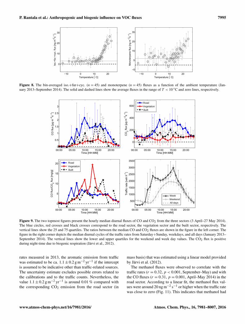
Figure 8. The bin-averaged iso.+fur+cyc. (n= 45) and monoterpene (n= 45) fluxes as a function of the ambient temperature (Jan-uary 2013–September 2014). The solid and dashed lines show the average fluxes in the range of T < 10 ◦C and zero lines, respectively.
RoadVegetationBuilt
RoadVegetationBuilt
WeekWeekendAll days
Figure 9. The two topmost figures present the hourly median diurnal fluxes of CO and CO2 from the three sectors (3 April–27 May 2014).The blue circles, red crosses and black crosses correspond to the road sector, the vegetation sector and the built sector, respectively. Thevertical lines show the 25 and 75 quartiles. The ratios between the median CO and CO2 fluxes are shown in the figure in the left corner. Thefigure in the right corner depicts the median diurnal cycles of the traffic rates from Saturday+Sunday, weekdays, and all days (January 2013–September 2014). The vertical lines show the lower and upper quartiles for the weekend and week day values. The CO2 flux is positiveduring night-time due to biogenic respiration (Järvi et al., 2012).
rates measured in 2013, the aromatic emission from trafficwas estimated to be ca. 1.1± 0.2 g m−2 yr−1 if the interceptis assumed to be indicative other than traffic-related sources.The uncertainty estimate excludes possible errors related tothe calibrations and to the traffic counts. Nevertheless, thevalue 1.1± 0.2 g m−2 yr−1 is around 0.01 % compared withthe corresponding CO2 emission from the road sector (in
mass basis) that was estimated using a linear model providedby Järvi et al. (2012).
The methanol fluxes were observed to correlate with thetraffic rates (r = 0.32, p < 0.001, September–May) and withthe CO fluxes (r = 0.31, p = 0.001, April–May 2014) in theroad sector. According to a linear fit, the methanol flux val-ues were around 20 ng m−2 s−1 or higher when the traffic ratewas close to zero (Fig. 11). This indicates that methanol had
www.atmos-chem-phys.net/16/7981/2016/ Atmos. Chem. Phys., 16, 7981–8007, 2016

7996 P. Rantala et al.: Anthropogenic and biogenic influence on VOC fluxes
RoadLinear fit
RoadLinear fit
VegetationLinear fit
BuiltLinear fit
Figure 10. The CO fluxes against the traffic rates and the CO2 fluxes from the road, vegetation and built sector (measured during April–May2014).
probably also other major sources than the traffic. This isalso supported by the fact that the average methanol fluxesfrom weekend and weekdays were quite close to each other(Fig. 4), even though the traffic rates were clearly largerduring the weekdays (Fig. 9). However, we were not ableto identify any clear additional sources to the traffic exceptbiogenic emissions during summer. To support our claim,Langford et al. (2010) found that the traffic counts were ableto explain only a part of the observed methanol fluxes butother methanol sources remained unknown in that study aswell.
The other oxygenated hydrocarbon fluxes correlated alsowith the traffic rates. The ethanol+formic acid fluxes weresomewhat noisy and mostly close to the detection limit(Table 4) but the correlation between the measured fluxesand the traffic rates was still significant (r = 0.19, p <0.001, January 2013–September 2014). However, no cor-relation between the ethanol+formic acid and CO fluxeswas found. The corresponding correlation coefficients foracetone+propanal were 0.23 (p < 0.001, traffic) and 0.42(p < 0.001, CO). The correlation between the acetaldehydeand CO fluxes was 0.39 (p < 0.001) and between the ac-etaldehyde flux and the traffic rates 0.30 (p < 0.001). The
methanol, acetaldehyde and acetone+propanal fluxes alsohad considerable correlations with each other, indicating thatthese compounds had probably similar sources from the roadsector. The correlation coefficients between the methanoland acetaldehyde fluxes and methanol and acetone+propanalfluxes were 0.52 and 0.38, respectively (p < 0.001, measure-ments from September–May). The period between Septem-ber and May was used instead of winter, i.e. non-growingseason, to have a reasonable amount of data.
The iso.+fur.+cyc. fluxes measured during September–May had a weak but a significant correlation (r = 0.20,p < 0.001) with the traffic rates (Fig. 11). Moreover, the av-erage iso.+fur.+cyc. flux was positive during winter (Ta-ble 4), indicating that some of the iso.+fur.+cyc. fluxesoriginate from anthropogenic sources. A correlation betweenthe iso.+fur.+cyc. fluxes and the traffic rates has also beenearlier observed by Valach et al. (2015). A correlation be-tween the iso.+fur.+cyc. and the CO fluxes was signifi-cant (r = 0.37, p < 0.001) also indicating a traffic-relatedsource. However, one should note that isoprene is also emit-ted from biogenic sources and this component is difficult todistinguish from the measured fluxes. If the data from wintermonths was only used, no relation between iso.+fur.+cyc.
Atmos. Chem. Phys., 16, 7981–8007, 2016 www.atmos-chem-phys.net/16/7981/2016/

P. Rantala et al.: Anthropogenic and biogenic influence on VOC fluxes 7997
RoadLinear fitRoadLinear fit
RoadLinear fit
RoadLinear fit
Figure 11. The traffic rates against the methanol (bin-averages,n= 15), iso.+fur.+cyc. (bin-averages, n= 15) and aromatic fluxes(benzene+toluene+C2-benzenes, bin-averages, n= 30) from theroad section. The linear correlations between the methanol,iso.+fur.+cyc. and aromatic fluxes and the traffic rates were 0.24(June–August)/0.32 (September–May), 0.20 and 0.38, respectively(p < 0.001).
fluxes and the traffic rates was found. On the other hand, theamount of data was also quite limited from those months (Ta-ble 4).
The monoterpene fluxes had only a weak correlation withthe traffic rates (r = 0.14, p = 0.001). However, even theweak correlation might also have been a result of the in-creased biogenic emissions as they have a similar kind ofdiurnal cycle compared with the traffic rates. The biogenicinfluence would be possible to eliminate by dividing themonoterpene fluxes into different temperature classes, butthe amount of data was too small for that kind of analysis.Thus, the possible monoterpene emissions from the trafficremained unknown, although the rush hour peak in the diur-nal concentration cycle (Fig. 6) indicated traffic-related emis-sions.
The acetonitrile fluxes had no correlation with the trafficrates. This was expected as the only considerable acetoni-trile fluxes were observed from the built sector (Fig. 3). Theacetonitrile emissions from the traffic should also be smallcompared to toluene or benzene emissions (e.g. Karl et al.,2009 and references therein).
Overall, the observed correlations were relatively low forall the VOCs. One explanation is that the fluxes were noisy,reducing therefore also the corresponding correlation coeffi-cients. On the other hand, the low correlations may also in-dicate multiple sources for many of the VOCs, decreasingtherefore the correlations between the fluxes and, for exam-ple, the traffic rates, and thus making the VOC source analy-sis very challenging.
3.2.2 Biogenic emissions
Nordbo et al. (2012a) observed that the urban CO2 fluxesare clearly dependent on the fraction of vegetated land areain the flux footprint. Moreover, Järvi et al. (2012) observedthat at our measurement site the vegetation sector is a sinkfor CO2 during summer (see also Fig. 9). Thus, the bio-genic VOC emissions could be expected to occur at the site.For iso.+fur.+cyc., the biogenic contribution was clear, andan anticorrelation (r =−0.53,p < 0.001) between the CO2and iso.+fur.+cyc. fluxes were observed from the vegeta-tion sector during the summer. The iso.+fur.+cyc. fluxeswere also affected by the ambient temperature with the smallfluxes associated with the low temperatures (Fig. 8). Also themethanol fluxes had a high anticorrelation with the carbondioxide fluxes from the vegetation sector between June andAugust (r =−0.59, p < 0.001), indicating a biogenic sourceas well.
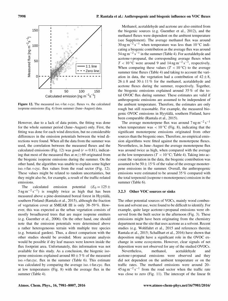
The iso.+fur.+cyc. fluxes were fitted against the empiri-cal isoprene algorithm (Eq. 4) to obtain the emission at stan-dard conditions. Thus, the only free parameter in the fittingwas the emission potential E0. It has been shown before thatthe emission potential of isoprene might have a seasonal cy-cle with a maximum during midsummer (e.g. in the case ofaspen: Fuentes et al., 1999; see also Rantala et al., 2015).
www.atmos-chem-phys.net/16/7981/2016/ Atmos. Chem. Phys., 16, 7981–8007, 2016
7998 P. Rantala et al.: Anthropogenic and biogenic influence on VOC fluxes
0 50 100 150
0
50
100
150
Calculated emission [ng m−2s−1]
Mea
sure
d flu
x [n
g m
−2 s−
1 ]
1:1 lineZero line
Figure 12. The measured iso.+fur.+cyc. fluxes vs. the calculatedisoprene emissions (Eq. 4) from summer (June–August) data.
However, due to a lack of data points, the fitting was donefor the whole summer period (June–August) only. First, thefitting was done for each wind direction, but no considerabledifferences in the emission potentials between the wind di-rections were found. When all the data from the summer wasused, the correlation between the measured fluxes and thecalculated emissions (Fig. 12) was good (r = 0.81), indicat-ing that most of the measured flux at m/z 69 originated fromthe biogenic isoprene emissions during the summer. On theother hand, the algorithm was unable to explain some higheriso.+fur.+cyc. flux values from the road sector (Fig. 12).These values might be related to random uncertainties, butthey might also be, for example, a result of the traffic-relatedemissions.
The calculated emission potential (E0 = 125±5 ng m−2 s−1) is roughly twice as high that has beenmeasured above a pine-dominated boreal forest in Hyytiälä,southern Finland (Rantala et al., 2015), although the fractionof vegetation cover at SMEAR III is only 38–59 %. How-ever, this was expected as the urban vegetation consists ofmostly broadleaved trees that are major isoprene emitters(e.g. Guenther et al., 2006). On the other hand, one shouldnote that the emission potentials were determined abovea rather heterogeneous terrain with multiple tree species(e.g. botanical garden). Thus, a direct comparison with theother studies should be avoided. More accurate analysiswould be possible if dry leaf masses were known inside theflux footprint area. Unfortunately, this information was notavailable for this study. As a conclusion, the biogenic iso-prene emissions explained around 80± 5 % of the measurediso.+fur.cyc. flux in the summer (Table 6). This estimatewas calculated by comparing the average iso.+fur.cyc. fluxat low temperatures (Fig. 8) with the average flux in thesummer (Table 4).
Methanol, acetaldehyde and acetone are also emitted fromthe biogenic sources (e.g. Guenther et al., 2012), and themethanol fluxes were dependent on the ambient temperature(see Supplement). The average methanol flux was around30 ng m−2 s−1 when temperature was less than 10 ◦C indi-cating a biogenic contribution as the average flux was around54 ng m−2 s−1 in the summer (Table 4). For acetaldehyde andacetone+propanal, the corresponding average fluxes whenT < 10 ◦C were around 9 and 14 ng m−2 s−1, respectively.When comparing these values (T < 10 ◦C) to the averagesummer time fluxes (Table 4) and taking to account the vari-ation in data, the vegetation had a contribution of 42± 8,26± 8 and 30± 11 % for the methanol, acetaldehyde andacetone fluxes during the summer, respectively. Together,the biogenic emissions explained around 35 % of the to-tal OVOC flux during summer. These estimates are valid ifanthropogenic emissions are assumed to be independent ofthe ambient temperature. Therefore, the estimates are onlyrough but still reasonable. For example, the measured bio-genic OVOC emissions in Hyytiälä, southern Finland, havebeen comparable (Rantala et al., 2015).
The average monoterpene flux was around 7 ng m−2 s−1
when temperature was < 10 ◦C (Fig. 8), indicating that thesignificant monoterpene emissions originated from othersources than the biogenic ones. Therefore, no empirical emis-sion algorithms were fitted against the monoterpene fluxes.Nevertheless, in June–August the average monoterpene fluxwas around twice as high, when compared with the averageat the low temperatures (T < 10 ◦C; Table 4). Taking into ac-count the variation in the data, the biogenic contribution wasassumed to be 50± 15 % of the value of the average monoter-pene emissions in the summer. Overall, the anthropogenicemissions were estimated to be around 35 % compared withthe total terpenoid (isoprene+monoterpenes) emission in thesummer (Table 6).
3.2.3 Other VOC sources or sinks
The other potential sources of VOCs, mainly wood combus-tion and solvent use, were found to be difficult to identify. Forexample, quite large acetone+propanal emissions were ob-served from the built sector in the afternoon (Fig. 3). Theseemissions might have been originating from the chemistrydepartment near the site that uses acetone as a solvent. Recentstudies (e.g. Wohlfahrt et al., 2015 and references therein;Rantala et al., 2015; Schallhart et al., 2016) have shown thatdeposition might have a significant role in the OVOC ex-change in some ecosystems. However, clear signals of netdeposition were not observed for any of the studied OVOCs.
Nevertheless, methanol, acetaldehyde andacetone+propanal emissions were observed and theydid not dependent on the ambient temperature or on thetraffic rates. The methanol emissions were around 20–45 ng m−2 s−1 from the road sector when the traffic ratewas close to zero (Fig. 11). The intercept of the linear fit
Atmos. Chem. Phys., 16, 7981–8007, 2016 www.atmos-chem-phys.net/16/7981/2016/
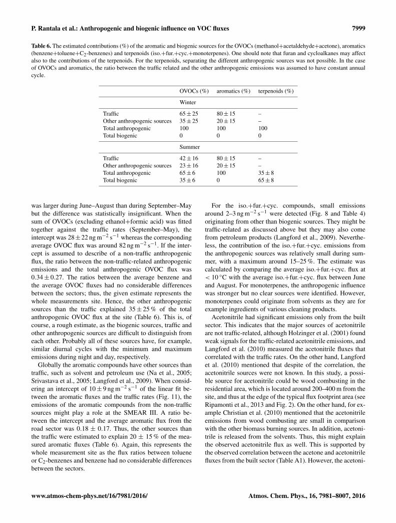
P. Rantala et al.: Anthropogenic and biogenic influence on VOC fluxes 7999
Table 6. The estimated contributions (%) of the aromatic and biogenic sources for the OVOCs (methanol+acetaldehyde+acetone), aromatics(benzene+toluene+C2-benzenes) and terpenoids (iso.+fur.+cyc.+monoterpenes). One should note that furan and cycloalkanes may affectalso to the contributions of the terpenoids. For the terpenoids, separating the different anthropogenic sources was not possible. In the caseof OVOCs and aromatics, the ratio between the traffic related and the other anthropogenic emissions was assumed to have constant annualcycle.
OVOCs (%) aromatics (%) terpenoids (%)
Winter
Traffic 65± 25 80± 15 –Other anthropogenic sources 35± 25 20± 15 –Total anthropogenic 100 100 100Total biogenic 0 0 0
Summer
Traffic 42± 16 80± 15 –Other anthropogenic sources 23± 16 20± 15 –Total anthropogenic 65± 6 100 35± 8Total biogenic 35± 6 0 65± 8
was larger during June–August than during September–Maybut the difference was statistically insignificant. When thesum of OVOCs (excluding ethanol+formic acid) was fittedtogether against the traffic rates (September–May), theintercept was 28±22 ng m−2 s−1 whereas the correspondingaverage OVOC flux was around 82 ng m−2 s−1. If the inter-cept is assumed to describe of a non-traffic anthropogenicflux, the ratio between the non-traffic-related anthropogenicemissions and the total anthropogenic OVOC flux was0.34± 0.27. The ratios between the average benzene andthe average OVOC fluxes had no considerable differencesbetween the sectors; thus, the given estimate represents thewhole measurements site. Hence, the other anthropogenicsources than the traffic explained 35± 25 % of the totalanthropogenic OVOC flux at the site (Table 6). This is, ofcourse, a rough estimate, as the biogenic sources, traffic andother anthropogenic sources are difficult to distinguish fromeach other. Probably all of these sources have, for example,similar diurnal cycles with the minimum and maximumemissions during night and day, respectively.
Globally the aromatic compounds have other sources thantraffic, such as solvent and petroleum use (Na et al., 2005;Srivastava et al., 2005; Langford et al., 2009). When consid-ering an intercept of 10± 9 ng m−2 s−1 of the linear fit be-tween the aromatic fluxes and the traffic rates (Fig. 11), theemissions of the aromatic compounds from the non-trafficsources might play a role at the SMEAR III. A ratio be-tween the intercept and the average aromatic flux from theroad sector was 0.18 ± 0.17. Thus, the other sources thanthe traffic were estimated to explain 20 ± 15 % of the mea-sured aromatic fluxes (Table 6). Again, this represents thewhole measurement site as the flux ratios between tolueneor C2-benzenes and benzene had no considerable differencesbetween the sectors.
For the iso.+fur.+cyc. compounds, small emissionsaround 2–3 ng m−2 s−1 were detected (Fig. 8 and Table 4)originating from other than biogenic sources. They might betraffic-related as discussed above but they may also comefrom petroleum products (Langford et al., 2009). Neverthe-less, the contribution of the iso.+fur.+cyc. emissions fromthe anthropogenic sources was relatively small during sum-mer, with a maximum around 15–25 %. The estimate wascalculated by comparing the average iso.+fur.+cyc. flux at< 10 ◦C with the average iso.+fur.+cyc. flux between Juneand August. For monoterpenes, the anthropogenic influencewas stronger but no clear sources were identified. However,monoterpenes could originate from solvents as they are forexample ingredients of various cleaning products.
Acetonitrile had significant emissions only from the builtsector. This indicates that the major sources of acetonitrileare not traffic-related, although Holzinger et al. (2001) foundweak signals for the traffic-related acetonitrile emissions, andLangford et al. (2010) measured the acetonitrile fluxes thatcorrelated with the traffic rates. On the other hand, Langfordet al. (2010) mentioned that despite of the correlation, theacetonitrile sources were not known. In this study, a possi-ble source for acetonitrile could be wood combusting in theresidential area, which is located around 200–400 m from thesite, and thus at the edge of the typical flux footprint area (seeRipamonti et al., 2013 and Fig. 2). On the other hand, for ex-ample Christian et al. (2010) mentioned that the acetonitrileemissions from wood combusting are small in comparisonwith the other biomass burning sources. In addition, acetoni-trile is released from the solvents. Thus, this might explainthe observed acetonitrile flux as well. This is supported bythe observed correlation between the acetone and acetonitrilefluxes from the built sector (Table A1). However, the acetoni-
www.atmos-chem-phys.net/16/7981/2016/ Atmos. Chem. Phys., 16, 7981–8007, 2016
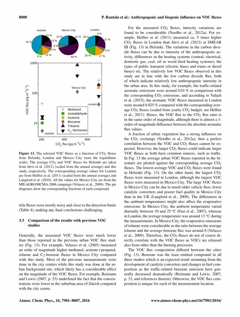
8000 P. Rantala et al.: Anthropogenic and biogenic influence on VOC fluxes
200 400 800
10
100
1000
CO2 flux [μg m−2s−1]
VO
C fl
ux [n
g m
−2 s−
1 ]
Helsinki
London
Mexico City
MethanolAcetaldehydeAcetoneBenzeneTolueneC
2−benzenes
42 %
9 % 15 %
5 %
13 %
15 % 24 %
6 %
49 %
21 % 29 %
20 % 17 %
5 %
21 %
9 %Helsinki Mexico City London
Figure 13. The selected VOC fluxes as a function of CO2 fluxesfrom Helsinki, London and Mexico City (note the logarithmicscale). The average CO2 and VOC fluxes for Helsinki are takenfrom Järvi et al. (2012) (scaled from the annual average) and thisstudy, respectively. The corresponding average values for Londonare from Helfter et al. (2011) (scaled from the annual average) andLangford et al. (2010). All the values for Mexico City are from theMILAGRO/MCMA-2006 campaign (Velasco et al., 2009). The piediagrams show the corresponding fractions of each compound.
trile fluxes were mostly noisy and close to the detection limits(Table 4), making any final conclusions challenging.
3.3 Comparison of the results with previous VOCstudies
Generally, the measured VOC fluxes were much lowerthan those reported in the previous urban VOC flux stud-ies (Fig. 13). For example, Velasco et al. (2005) measuredan order of magnitude higher methanol, acetone+propanal,toluene and C2-benzene fluxes in Mexico City comparedwith this study. Most of the previous measurements weredone in the city centres while this study was done at the ur-ban background site, which likely has a considerable effecton the magnitude of the VOC fluxes. For example, Reimannand Lewis (2007, p. 53) underlined the fact that the concen-trations were lower in the suburban area of Zürich comparedwith the city centre.
For the measured CO2 fluxes, intercity variations arefound to be considerable (Nordbo et al., 2012a). For ex-ample, Helfter et al. (2011) measured ca. 5 times higherCO2 fluxes in London than Järvi et al. (2012) at SMEARIII (Fig. 13) in Helsinki. The variations in the carbon diox-ide fluxes can be due to intensity of the anthropogenic ac-tivity, differences in the heating systems (central, electrical,domestic gas, coal, oil or wood fired heating systems), thetypes of public transport (electric buses and trams or dieselbuses) etc. The relatively low VOC fluxes observed in thisstudy are in line with the low carbon dioxide flux, bothof which indicate relatively low anthropogenic intensity inthe urban area. In this study, for example, the traffic-relatedaromatic emissions were around 0.01 % in comparison withthe corresponding CO2 emissions, and according to Valachet al. (2015), the aromatic VOC fluxes measured in Londonwere around 0.025 % compared with the corresponding aver-age CO2 fluxes (scaled from yearly CO2 budget, see Helfteret al., 2011). Hence, the VOC flux to the CO2 flux ratio isin the same order of magnitude, although there is almost a 1-order-of-magnitude difference between the absolute aromaticflux values.
A fraction of urban vegetation has a strong influence onthe CO2 exchange (Nordbo et al., 2012a); thus a perfectcorrelation between the VOC and CO2 fluxes cannot be ex-pected. However, the larger CO2 fluxes could indicate largerVOC fluxes as both have common sources, such as traffic.In Fig. 13 the average urban VOC fluxes reported in the lit-erature are plotted against the corresponding average CO2fluxes. The lowest average VOC and CO2 fluxes were foundin Helsinki (Fig. 13). On the other hand, the largest CO2fluxes were measured in London, although the largest VOCfluxes were measured in Mexico City. The large VOC fluxesin Mexico City can be due to much older vehicle fleet, fewercatalytic converters and poorer fuel quality in Mexico Citythan in the UK (Langford et al., 2009). The differences inthe ambient temperatures might also affect the evaporativeemissions. In Mexico City, the ambient temperature varieddiurnally between 10 and 25 ◦C (Fast et al., 2007), whereasin London, the average temperature was around 13 ◦C duringthe measurements. In Mexico City, the evaporative emissionsof toluene were considerable as the ratio between the averagetoluene and the average benzene flux was around 8 (Velascoet al., 2009). Therefore, the CO2-fluxes do not of course di-rectly correlate with the VOC fluxes as VOCs are releasedalso from other than the burning processes.
The VOC flux composition differed between the cities(Fig. 13). Benzene was the least emitted compound in allthree studies which is an expected result stemming from thedevelopment of catalytic converters and changes in fuel com-position as the traffic-related benzene emission have gen-erally decreased dramatically (Reimann and Lewis, 2007,p. 33, and references therein). Otherwise, the VOC flux com-position is unique for each of the measurement location.
Atmos. Chem. Phys., 16, 7981–8007, 2016 www.atmos-chem-phys.net/16/7981/2016/

P. Rantala et al.: Anthropogenic and biogenic influence on VOC fluxes 8001
4 Conclusions
We present results from the first urban VOC flux measure-ments in a northern city with cold winters. Out of 13 mea-sured mass-to-charge ratios, the fluxes were observed for 10(m/z 33, 42, 45, 47, 59, 69, 79, 81, 93 and 107). Previouspublished works have indicated the emissions of the samecompounds in urban VOC flux studies. The different landuse categories around the measurement site in different winddirections enabled us to analyse the different sources of vari-ous compounds differentiating between the traffic, vegetationand residential sources.
The VOC fluxes varied as a function of season. Methanolhad the highest fluxes in all seasons. The other OVOCs,toluene and C2-benzenes fluxes were of the same magni-tude with each other and had differences in the absoluteflux values between winter and summer. The iso.+fur.+cyc.fluxes were clearly higher during the summer than during thewinter, indicating a major contribution of biogenic isopreneemissions.
All compounds with the detectable fluxes illustrated con-tributions from anthropogenic sources at the site. The aro-matic compounds originated mostly from the traffic whereasfor the iso.+fur.+cyc. fluxes, the anthropogenic influencewas less important. However, even the small iso.+fur.+cyc.fluxes had a relatively large influence on the iso.+fur.+cyc.concentrations during the winter when the biogenic emissionis small. For monoterpenes, the anthropogenic influence waslarger, being of similar magnitude with the biogenic emis-sions in summer. The oxygenated VOCs originated fromthe traffic, vegetation and unknown anthropogenic sources,which probably included solvent use at the University cam-pus. Generally, the magnitude of the traffic-related OVOCemissions was estimated to be slightly higher compared withother anthropogenic sources. However, estimating the ex-act fraction was found to be difficult and uncertainties werelarge. Even in the urban background site, the biogenic activ-ity had a contribution to the total annual OVOC exchange.For methanol, the biogenic emissions explained around 40 %of the measured flux values during the summer.
On one hand, the measured VOC fluxes were much lowerthan have earlier been observed in the urban VOC flux stud-ies. On the other hand, most of the earlier urban VOC fluxstudies have been carried out in dense city centres, such asin London, whereas this study was done ca. 5 km from theHelsinki city centre in a semi-urban area. Moreover, the CO2fluxes have been observed to be relatively low at SMEAR IIIcompared with the other urban stations. However, the varia-tion of the CO2 flux can only partly explain the variation inthe VOC fluxes between the different urban areas.
The measured urban VOC fluxes showed considerablevariations between the different cities both in quantity andin quality. Thus, a general parameterization for the VOCexchange in the urban areas may be challenging. However,links between the VOC emissions and CO2 and the CO emis-sion provide indication of the processes which need to bedescribed by the parameterizations. To acquire this, a largerbody of concomitant measurements of VOC, CO and CO2fluxes may be needed.
5 Data availability
All data is available on request by the corresponding author.
www.atmos-chem-phys.net/16/7981/2016/ Atmos. Chem. Phys., 16, 7981–8007, 2016

8002 P. Rantala et al.: Anthropogenic and biogenic influence on VOC fluxes
Appendix A
Table A1. Correlation coefficients from each wind sector between VOC, CO, CO2 fluxes and the traffic rates (Tr, only from the road sector)using all available data (one percent of the highest and the lowest values were disregarded). Insignificant (p > 0.05) correlation coefficientsare not shown in the Table. For a comparison, the correlation coefficient between the CO2 fluxes and the traffic rates was calculated from thesame period with the CO fluxes (April–May 2014).
Road sector
m/z 33 m/z 42 m/z 45 m/z 47 m/z 59 m/z 69 m/z 79 m/z 81 m/z 93 m/z 107 CO CO2 Tr
m/z 33 1 – 0.52 0.31 0.38 0.33 0.29 0.21 0.30 0.33 0.31 0.31 0.30m/z 42 – 1 – – – 0.12 – – – – – – –m/z 45 0.52 – 1 0.32 0.44 0.44 0.31 0.13 0.33 0.35 0.39 0.33 0.30m/z 47 0.31 – 0.32 1 0.14 0.08 0.23 0.13 0.23 0.25 – 0.37 0.19m/z 59 0.38 – 0.44 0.14 1 0.31 0.23 0.19 0.24 0.34 0.42 0.15 0.23m/z 69 0.33 0.12 0.44 0.08 0.31 1 0.19 0.19 0.24 0.19 0.37 – 0.30m/z 79 0.29 – 0.31 0.23 0.23 0.19 1 – 0.26 0.25 0.35 0.21 0.17m/z 81 0.21 – 0.13 0.13 0.19 0.19 – 1 0.13 0.19 – 0.11 0.14m/z 93 0.30 – 0.33 0.23 0.24 0.24 0.26 0.13 1 0.38 0.37 0.37 0.30m/z 107 0.33 – 0.35 0.25 0.34 0.19 0.25 0.19 0.38 1 0.44 0.38 0.32CO 0.31 – 0.39 – 0.42 0.37 0.35 – 0.37 0.44 1 0.68 0.56CO2 0.31 – 0.33 0.37 0.15 – 0.21 0.11 0.37 0.38 0.68 1 0.43tr 0.30 – 0.30 0.19 0.23 0.30 0.17 0.14 0.30 0.32 0.56 0.43 1
Vegetation sector
m/z 33 m/z 42 m/z 45 m/z 47 m/z 59 m/z 69 m/z 79 m/z 81 m/z 93 m/z 107 CO CO2
m/z 33 1 0.10 0.55 0.29 0.37 0.34 0.14 0.23 0.23 0.21 0.28 −0.29m/z 42 0.10 1 – 0.08 0.09 – – – – 0.09 – –m/z 45 0.55 – 1 0.35 0.42 0.35 0.14 0.18 0.19 0.22 0.34 −0.12m/z 47 0.29 0.08 0.35 1 0.25 – 0.19 0.13 0.19 0.24 0.18 0.18m/z 59 0.37 0.09 0.42 0.25 1 0.25 0.18 0.17 0.19 0.18 0.39 −0.10m/z 69 0.34 – 0.35 – 0.25 1 – 0.13 – 0.18 – -0.44m/z 79 0.14 – 0.14 0.19 0.18 – 1 0.08 0.13 0.14 – –m/z 81 0.23 – 0.18 0.13 0.17 0.13 0.08 1 0.13 – 0.20 -0.17m/z 93 0.23 – 0.19 0.19 0.19 – 0.13 0.13 1 0.17 0.24 –m/z 107 0.21 0.09 0.22 0.24 0.18 0.18 0.14 – 0.17 1 0.22 0.09CO 0.28 – 0.34 0.18 0.39 – – 0.20 0.24 0.22 1 0.28CO2 −0.29 – −0.12 0.18 −0.10 −0.44 – −0.17 – 0.09 0.28 1
Built sector
m/z 33 m/z 42 m/z 45 m/z 47 m/z 59 m/z 69 m/z 79 m/z 81 m/z 93 m/z 107 CO CO2
m/z 33 1 0.21 0.45 0.37 0.30 0.27 – 0.24 0.32 – – –m/z 42 0.21 1 0.35 – 0.40 – – – 0.19 0.21 – –m/z 45 0.45 0.35 1 0.48 0.25 0.19 – – 0.26 – – –m/z 47 0.37 – 0.48 1 0.22 – 0.33 – 0.35 – – –m/z 59 0.30 0.40 0.25 0.22 1 0.18 0.27 0.18 0.32 – 0.75 –m/z 69 0.27 – 0.19 – 0.18 1 0.33 – 0.38 0.19 – −0.32m/z 79 – – – 0.33 0.27 0.33 1 – 0.23 – – –m/z 81 0.24 – – – 0.18 – – 1 – – – –m/z 93 0.32 0.19 0.26 0.35 0.32 0.38 0.23 – 1 0.40 – –m/z 107 – 0.21 – – – 0.19 – – 0.40 1 – –CO – 0.52 0.60 0.55 0.53 – – – – – 1 0.49CO2 – – – – – −0.32 – – – – 0.49 1
Atmos. Chem. Phys., 16, 7981–8007, 2016 www.atmos-chem-phys.net/16/7981/2016/

P. Rantala et al.: Anthropogenic and biogenic influence on VOC fluxes 8003
Table A2. The average VOC fluxes from the different seasons compared with the corresponding benzene fluxes (Table 4). The values in theparenthesis represent 95 % confidence intervals.
m/z 33 m/z 42 m/z 45 m/z 47 m/z 59 m/z 69 m/z 79 m/z 81 m/z 93 m/z 107
January 2013–September 2014
8.2 (±1.0) 0.13 (±0.03) 1.9 (±0.2) 4.0 (±0.5) 3.0 (±0.4) 1.5 (±0.2) 1 2.0 (±0.3) 2.6 (±0.3) 3.0 (±0.4)
Winter
4.8 (±1.9) – 0.7 (±0.3) 6.3 (±2.3) 2.4 (±0.9) 0.3 (±0.2) 1 1.2 (±0.6) 2.7 (±0.9) 3.4 (±1.2)
Spring
9.1 (±1.7) 0.20 (±0.05) 1.9 (±0.4) 4.6 (±1.0) 2.9 (±0.6) 0.9 (±0.2) 1 1.6 (±0.4) 2.4 (±0.5) 2.9 (±0.6)
Summer
11.2 (±2.0) 0.13 (±0.05) 2.4 (±0.4) 3.0 (±0.7) 4.3 (±0.8) 3.0 (±0.6) 1 2.9 (±0.6) 2.7 (±0.5) 2.9 (±0.6)
Autumn
6.0 (±1.8) 0.18 (±0.08) 2.2 (±0.7) 3.8 (±1.2) 2.6 (±0.9) 1.8 (±0.6) 1 2.3 (±1.0) 2.4 (±1.1) 2.7 (±1.2)
www.atmos-chem-phys.net/16/7981/2016/ Atmos. Chem. Phys., 16, 7981–8007, 2016

8004 P. Rantala et al.: Anthropogenic and biogenic influence on VOC fluxes
The Supplement related to this article is available onlineat doi:10.5194/acp-16-7981-2016-supplement.
Acknowledgements. We acknowledge the support from the Doc-toral programme of atmospheric sciences, and from the Academyof Finland (ICOS-Finland 281255 and ICOS-ERIC 281250), andfrom the Academy of Finland through its Centre of Excellenceprogram (Project No 272041 and 125238). We thank two anony-mous reviewers for useful comments that helped improve themanuscript. We thank Alessandro Franchin, Sigfried Schoesberger,Simon Schallhart and Lauri Ahonen for their help in carrying thePTR-MS between our laboratory and the measurement site. Fi-nally, we thank all the people who made the ancillary data available.
Edited by: T. Karl
References
Ammann, C., Brunner, A., Spirig, C., and Neftel, A.: Technicalnote: Water vapour concentration and flux measurements withPTR-MS, Atmos. Chem. Phys., 6, 4643–4651, doi:10.5194/acp-6-4643-2006, 2006.
Atkinson, R.: Atmospheric chemistry of VOCs and NOx, Atmos.Environ., 34, 2063–2101, 2000.
Atkinson, R. and Arey, J.: Gas-phase tropospheric chemistry of bio-genic volatile organic compounds: a review, Atmos. Environ., 37,Supplement 2, 197–219, 2003.
Aubinet, M., Vesala, T., and Papale, D.: Eddy Covariance: A Prac-tical Guide to Measurement and Data Analysis, Springer Atmo-spheric Sciences, Netherlands, 2012.
Borbon, A., Fontaine, H., Veillerot, M., Locoge, N., Galloo, J., andGuillermo, R.: An investigation into the traffic-related fraction ofisoprene at an urban location, Atmos. Environ., 35, 3749–3760,2001.
Borbon, A., Gilman, J. B., Kuster, W. C., Grand, N., Chevaillier, S.,Colomb, A., Dolgorouky, C., Gros, V., Lopez, M., Sarda-Esteve,R., Holloway, J., Stutz, J., Petetin, H., McKeen, S., Beekmann,M., Warneke, C., Parrish, D. D., and de Gouw, J. A.: Emissionratios of anthropogenic volatile organic compounds in northernmid-latitude megacities: Observations versus emission invento-ries in Los Angeles and Paris, J. Geophys. Res.-Atmos., 118,2041–2057, 2013.
Calfapietra, C., Fares, S., Manes, F., Morani, A., Sgrigna, G.,and Loreto, F.: Role of Biogenic Volatile Organic Compounds(BVOC) emitted by urban trees on ozone concentration in cities:A review, Environ. Pollut., 183, 71–80, 2013.
Caplain, I., Cazier, F., Nouali, H., Mercier, A., Déchaux, J.-C., Nol-let, V., Joumard, R., André, J.-M., and Vidon, R.: Emissions ofunregulated pollutants from European gasoline and diesel pas-senger cars, Atmos. Environ., 40, 5954–5966, 2006.
Christian, T. J., Yokelson, R. J., Cárdenas, B., Molina, L. T., En-gling, G., and Hsu, S.-C.: Trace gas and particle emissions fromdomestic and industrial biofuel use and garbage burning in cen-tral Mexico, Atmos. Chem. Phys., 10, 565–584, doi:10.5194/acp-10-565-2010, 2010.
de Gouw, J. and Warneke, C.: Measurements of volatile organiccompounds in the earth’s atmosphere using proton-transfer-reaction mass spectrometry, Mass Spectrom. Rev., 26, 223–257,2007.
De Gouw, J., Warneke, C., Parrish, D., Holloway, J., Trainer, M.,and Fehsenfeld, F.: Emission sources and ocean uptake of ace-tonitrile (CH3CN) in the atmosphere, J. Geophys. Res.-Atmos.,108, D11, 1doi:10.1029/2002JD002897, 2003.
Drebs, A., Nordlund, A., Karlsson, P., Helminen, J., and Rissa-nen, P.: Tilastoja Suomen ilmastosta 1971–2000 [Climatologicalstatistics of Finland 1971–2000], Finnish Meteorological Insti-tute, Helsinki, 2002.
Dunne, E., Galbally, I. E., Lawson, S., and Patti, A.: Interference inthe PTR-MS measurement of acetonitrile at m/z 42 in pollutedurban air – A study using switchable reagent ion PTR-MS, Int. J.Mass Spectrom., 319–320, 40–47, 2012.
Durana, N., Navazo, M., Gomez, M., Alonso, L., García, J., Ilardia,J., Gangoiti, G., and Iza, J.: Long term hourly measurement of62 non-methane hydrocarbons in an urban area: Main results andcontribution of non-traffic sources, Atmos. Environ., 40, 2860–2872, 2006.
Famulari, D., Nemitz, E., Marco, C. D., Phillips, G. J., Thomas,R., House, E., and Fowler, D.: Eddy-covariance measurementsof nitrous oxide fluxes above a city, Agr. Forest Meteorol., 150,786–793, 2010.
Farrauto, R. J. and Heck, R. M.: Catalytic converters: state of the artand perspectives, Catalysis Today, 51, 351–360, 1999.
Fast, J. D., de Foy, B., Acevedo Rosas, F., Caetano, E., Carmichael,G., Emmons, L., McKenna, D., Mena, M., Skamarock, W.,Tie, X., Coulter, R. L., Barnard, J. C., Wiedinmyer, C., andMadronich, S.: A meteorological overview of the MILA-GRO field campaigns, Atmos. Chem. Phys., 7, 2233–2257,doi:10.5194/acp-7-2233-2007, 2007.
Foken, T. and Wichura, B.: Tools for quality assessment of surface-based flux measurements, Agr. Forest Meteorol., 78, 83–105,1996.
Fuentes, J. D., Wang, D., and Gu, L.: Seasonal Variations in Iso-prene Emissions from a Boreal Aspen Forest, J. Appl. Meteorol.,38, 855–869, 1999.
Guenther, A. B.: Seasonal and spatial variations in natural volatileorganic compound emissions, Ecol. Appl., 7, 34–45, 1997.
Guenther, A. B., Monson, R. K., and Fall, R.: Isoprene andMonoterpene Emission Rate Variability: Observations With Eu-calyptus and Emission Rate Algorithm Development, J. Geo-phys. Res., 96, 10799–10808, 1991.
Guenther, A. B., Zimmerman, P. R., Harley, P. C., Monson, R. K.,and Fall, R.: Isoprene and Monoterpene Emission Rate Variabil-ity: Model Evaluations and Sensitivity Analyses, J. Geophys.Res., 98, 12609–12617, 1993.
Guenther, A., Karl, T., Harley, P., Wiedinmyer, C., Palmer, P. I.,and Geron, C.: Estimates of global terrestrial isoprene emissionsusing MEGAN (Model of Emissions of Gases and Aerosols fromNature), Atmos. Chem. Phys., 6, 3181–3210, doi:10.5194/acp-6-3181-2006, 2006.
Guenther, A. B., Jiang, X., Heald, C. L., Sakulyanontvittaya, T.,Duhl, T., Emmons, L. K., and Wang, X.: The Model of Emissionsof Gases and Aerosols from Nature version 2.1 (MEGAN2.1): anextended and updated framework for modeling biogenic emis-
Atmos. Chem. Phys., 16, 7981–8007, 2016 www.atmos-chem-phys.net/16/7981/2016/

P. Rantala et al.: Anthropogenic and biogenic influence on VOC fluxes 8005
sions, Geosci. Model Dev., 5, 1471–1492, doi:10.5194/gmd-5-1471-2012, 2012.
Harrison, R. M., Dall’Osto, M., Beddows, D. C. S., Thorpe, A.J., Bloss, W. J., Allan, J. D., Coe, H., Dorsey, J. R., Gallagher,M., Martin, C., Whitehead, J., Williams, P. I., Jones, R. L., Lan-gridge, J. M., Benton, A. K., Ball, S. M., Langford, B., Hewitt,C. N., Davison, B., Martin, D., Petersson, K. F., Henshaw, S. J.,White, I. R., Shallcross, D. E., Barlow, J. F., Dunbar, T., Davies,F., Nemitz, E., Phillips, G. J., Helfter, C., Di Marco, C. F., andSmith, S.: Atmospheric chemistry and physics in the atmosphereof a developed megacity (London): an overview of the REPAR-TEE experiment and its conclusions, Atmos. Chem. Phys., 12,3065–3114, doi:10.5194/acp-12-3065-2012, 2012.
Helfter, C., Famulari, D., Phillips, G. J., Barlow, J. F., Wood, C. R.,Grimmond, C. S. B., and Nemitz, E.: Controls of carbon dioxideconcentrations and fluxes above central London, Atmos. Chem.Phys., 11, 1913–1928, doi:10.5194/acp-11-1913-2011, 2011.
Hellén, H., Hakola, H., and Laurila, T.: Determination of sourcecontributions of NMHCs in Helsinki (60◦N, 25◦E) using chem-ical mass balance and the Unmix multivariate receptor models,Atmos. Environ., 37, 1413–1424, 2003.
Hellén, H., Hakola, H., Pirjola, L., Laurila, T., and Pystynen, K.-H.:Ambient air concentrations, source profiles, and source appor-tionment of 71 different C2-C10 volatile organic compounds inurban and residential areas of Finland, Environ. Sci. Technol.,40, 103–108, 2006.
Hellén, H., Tykkä, T., and Hakola, H.: Importance of monoterpenesand isoprene in urban air in northern Europe, Atmos. Environ.,59, 59–66, 2012.
Holzinger, R., Warneke, C., Hansel, A., Jordan, A., Lindinger, W.,Scharffe, D. H., Schade, G., and Crutzen, P. J.: Biomass burn-ing as a source of formaldehyde, acetaldehyde, methanol, ace-tone, acetonitrile, and hydrogen cyanide, Geophys. Res. Lett., 26,1161–1164, 1999.
Holzinger, R., Jordan, A., Hansel, A., and Lindinger, W.: Automo-bile Emissions of Acetonitrile: Assessment of its Contribution tothe Global Source, J. Atmos. Chem., 38, 187–193, 2001.
Horst, T. W.: A simple formula for attenuation of eddy fluxes mea-sured with first-order-response scalar sensors, Bound.-Lay. Me-teorol., 82, 219–233, 1997.
Ibrom, A., Dellwik, E., Larsen, S. E., and Pilegaard, K.: On theuse of the Webb–Pearman–Leuning theory for closed-path eddycorrelation measurements, Tellus B, 59, 937–946, 2007.
Järvi, L., Hannuniemi, H., Hussein, T., Junninen, H., Aalto, P. P.,Hillamo, R., Mäkelä, T., Keronen, P., Siivola, E., Vesala, T., andKulmala, M.: The urban measurement station SMEAR III: Con-tinuous monitoring of air pollution and surface-atmosphere inter-actions in Helsinki, Finland, Boreal Environ. Res., 14, 86–109,2009a.
Järvi, L., Mammarella, I., Eugster, W., Ibrom, A., Siivola, E., Dell-wik, E., Keronen, P., Burba, G., and Vesala, T.: Comparison ofnet CO2 fluxes measured with open-and closed-path infraredgas analyzers in an urban complex environment, Boreal Environ.Res., 14, 499–514, 2009b.
Järvi, L., Nordbo, A., Junninen, H., Riikonen, A., Moilanen, J.,Nikinmaa, E., and Vesala, T.: Seasonal and annual variation ofcarbon dioxide surface fluxes in Helsinki, Finland, in 2006–2010,Atmos. Chem. Phys., 12, 8475–8489, doi:10.5194/acp-12-8475-2012, 2012.
Järvi, L., Grimmond, C. S. B., Taka, M., Nordbo, A., Setä”a, H.,and Strachan, I. B.: Development of the Surface Urban Energyand Water Balance Scheme (SUEWS) for cold climate cities,Geosci. Model Dev., 7, 1691–1711, doi:10.5194/gmd-7-1691-2014, 2014.
Kajos, M. K., Rantala, P., Hill, M., Hellén, H., Aalto, J., Patokoski,J., Taipale, R., Hoerger, C. C., Reimann, S., Ruuskanen, T. M.,Rinne, J., and Petäjä, T.: Ambient measurements of aromaticand oxidized VOCs by PTR-MS and GC-MS: intercompari-son between four instruments in a boreal forest in Finland, At-mos. Meas. Tech., 8, 4453–4473, doi:10.5194/amt-8-4453-2015,2015.
Kansal, A.: Sources and reactivity of NMHCs and VOCs in the at-mosphere: A review, J. Hazard. Mater., 166, 17–26, 2009.
Karl, T., Spirig, C., Rinne, J., Stroud, C., Prevost, P., Greenberg, J.,Fall, R., and Guenther, A.: Virtual disjunct eddy covariance mea-surements of organic compound fluxes from a subalpine forestusing proton transfer reaction mass spectrometry, Atmos. Chem.Phys., 2, 279–291, doi:10.5194/acp-2-279-2002, 2002.
Karl, T., Apel, E., Hodzic, A., Riemer, D. D., Blake, D. R., andWiedinmyer, C.: Emissions of volatile organic compounds in-ferred from airborne flux measurements over a megacity, Atmos.Chem. Phys., 9, 271–285, doi:10.5194/acp-9-271-2009, 2009.
Karl, T., Hansel, A., Cappellin, L., Kaser, L., Herdlinger-Blatt,I., and Jud, W.: Selective measurements of isoprene and 2-methyl-3-buten-2-ol based on NO+ ionization mass spectrom-etry, Atmos. Chem. Phys., 12, 11877–11884, doi:10.5194/acp-12-11877-2012, 2012.
Kazil, J., Stier, P., Zhang, K., Quaas, J., Kinne, S., O’Donnell, D.,Rast, S., Esch, M., Ferrachat, S., Lohmann, U., and Feichter,J.: Aerosol nucleation and its role for clouds and Earth’s ra-diative forcing in the aerosol-climate model ECHAM5-HAM,Atmos. Chem. Phys., 10, 10733–10752, doi:10.5194/acp-10-10733-2010, 2010.
Kormann, R. and Meixner, F. X.: An analytical footprint model fornon-neutral stratification, Bounda.-Lay. Meteorol., 99, 207–224,2001.
Kulmala, M., Suni, T., Lehtinen, K. E. J., Dal Maso, M., Boy, M.,Reissell, A., Rannik, Ü., Aalto, P., Keronen, P., Hakola, H., Bäck,J., Hoffmann, T., Vesala, T., and Hari, P.: A new feedback mecha-nism linking forests, aerosols, and climate, Atmos. Chem. Phys.,4, 557–562, doi:10.5194/acp-4-557-2004, 2004.
Langford, B., Davison, B., Nemitz, E., and Hewitt, C. N.: Mix-ing ratios and eddy covariance flux measurements of volatile or-ganic compounds from an urban canopy (Manchester, UK), At-mos. Chem. Phys., 9, 1971–1987, doi:10.5194/acp-9-1971-2009,2009.
Langford, B., Nemitz, E., House, E., Phillips, G. J., Famulari,D., Davison, B., Hopkins, J. R., Lewis, A. C., and Hewitt, C.N.: Fluxes and concentrations of volatile organic compoundsabove central London, UK, Atmos. Chem. Phys., 10, 627–645,doi:10.5194/acp-10-627-2010, 2010.
Langford, B., Acton, W., Ammann, C., Valach, A., and Nemitz, E.:Eddy-covariance data with low signal-to-noise ratio: time-lag de-termination, uncertainties and limit of detection, Atmos. Meas.Tech., 8, 4197–4213, doi:10.5194/amt-8-4197-2015, 2015.
Lee, A., Goldstein, A. H., Keywood, M. D., Gao, S., Varut-bangkul, V., Bahreini, R., Ng, N. L., Flagan, R. C., and Seinfeld,J. H.: Gas-phase products and secondary aerosol yields from the
www.atmos-chem-phys.net/16/7981/2016/ Atmos. Chem. Phys., 16, 7981–8007, 2016
8006 P. Rantala et al.: Anthropogenic and biogenic influence on VOC fluxes
ozonolysis of ten different terpenes, J. Geophys. Res.-Atmos.,111, D7, doi:10.1029/2005JD006437, 2006.
Lilleberg, I. and Hellman, T.: Liikenteen kehitys Helsingissävuonna 2011, Helsinki City Planning Department 2011, 2011.
Lindinger, W., Hansel, A., and Jordan, A.: On-line monitoring ofvolatile organic compounds at pptv levels by means of Proton-Transfer-Reaction Mass Spectrometry (PTR-MS) – Medical ap-plications, food control and environmental research, Int. J. MassSpectr., 173, 191–241, 1998.
Mammarella, I., Launiainen, S., Grönholm, T., Keronen, P., Pumpa-nen, J., Rannik, Ü., and Vesala, T.: Relative Humidity Effect onthe High-Frequency Attenuation of Water Vapor Flux Measuredby a Closed-Path Eddy Covariance System, J. Atmos. Ocean.Tech., 26, 1856–1866, 2009.
Mammarella, I., Peltola, O., Nordbo, A., Järvi, L., and Rannik, Ü.:EddyUH: an advanced software package for eddy covariance fluxcalculation for a wide range of instrumentation and ecosystems,Atmos. Meas. Tech. Discuss., doi:10.5194/amt-2015-323, in re-view, 2016.
Misztal, P. K., Hewitt, C. N., Wildt, J., Blande, J. D., Eller, A. S. D.,Fares, S., Gentner, D. R., Gilman, J. B., Graus, M., Greenberg, J.,Guenther, A. B., Hansel, A., Harley, P., Huang, M., Jardine, K.,Karl, T., Kaser, L., Keutsch, F. N., Kiendler-Scharr, A., Kleist,E., Lerner, B. M., Li, T., Mak, J., Nölscher, A. C., Schnitzhofer,R., Sinha, V., Thornton, B., Warneke, C., Wegener, F., Werner,C., Williams, J., Worton, D. R., Yassaa, N., and Goldstein, A. H.:Atmospheric benzenoid emissions from plants rival those fromfossil fuels, Scientific reports, 5, 12064, doi:10.1038/srep12064,2015.
Moore, C. J.: Frequency Response Corrections for Eddy CorrelationSystems, Bound.-Lay. Meteorol., 37, 17–35, 1986.
Na, K., Moon, K.-C., and Kim, Y. P.: Source contribution to aro-matic VOC concentration and ozone formation potential in theatmosphere of Seoul, Atmos. Environ., 39, 5517–5524, 2005.
Niven, R. K.: Ethanol in gasoline: environmental impacts and sus-tainability review article, Renew. Sust. Energ. Rev., 9, 535–555,2005.
Nordbo, A., Järvi, L., Haapanala, S., Wood, C. R., andVesala, T.: Fraction of natural area as main predictor ofnet CO2 emissions from cities, Geophys. Res. Lett., 39, 20,doi:10.1029/2012GL053087, 2012a.
Nordbo, A., Järvi, L., and Vesala, T.: Revised eddy covariance fluxcalculation methodologies – effect on urban energy balance, Tel-lus B, 64, 18184 doi:10.3402/tellusb.v64i0.18184, 2012b.
Nordbo, A., Kekäläinen, P., Siivola, E., Lehto, R., Vesala, T., and Ti-monen, J.: Tube transport of water vapor with condensation anddesorption, Appl. Phys. Lett., 102, 19, doi:10.1063/1.4804639,2013.
Nordbo, A., Kekäläinen, P., Siivola, E., Mammarella, I., Timonen,J., and Vesala, T.: Sorption-Caused Attenuation and Delay of Wa-ter Vapor Signals in Eddy-Covariance Sampling Tubes and Fil-ters, J. Atmos. Ocean. Tech., 31, 2629–2649, 2014.
Paasonen, P., Asmi, A., Petäjä, T., Kajos, M. K., Äijälä, M., Junni-nen, H., Holst, T., Abbatt, J. P. D., Arneth, A., Birmili, W., vander Gon, H. A. C. D., Hamed, A., Hoffer, A., Laakso, L., Laak-sonen, A., Leaitch, W. R., Plass-Dülmer, C., C., P. S., Räisänen,P., Swietlicki, E., Wiedensohler, A., Worsnop, D. R., Kerminen,V.-M., and Kulmala, M.: Warming-induced increase in aerosol
number concentration likely to moderate climate change, Nat.Geosci. Lett., 12, 438–442, 2013.
Park, C., Schade, G. W., and Boedeker, I.: Flux measurements ofvolatile organic compounds by the relaxed eddy accumulationmethod combined with a GC-FID system in urban Houston,Texas, Atmos. Environ., 44, 2605–2614, 2010.
Park, J.-H., Goldstein, A., Timkovsky, J., Fares, S., Weber, R.,Karlik, J., and Holzinger, R.: Active atmosphere-ecosystem ex-change of the vast majority of detected volatile organic com-pounds, Science, 341, 643–647, 2013.
Patokoski, J., Ruuskanen, T. M., Hellén, H., Taipale, R., Grönholm,T., Kajos, M. K., Petäjä, T., Hakola, H., Kulmala, M., and Rinne,J.: Winter to spring transition and diurnal variation of vocs in Fin-land at an urban background site and a rural site, Boreal Environ.Res., 19, 79–103, 2014.
Patokoski, J., Ruuskanen, T. M., Kajos, M. K., Taipale, R., Rantala,P., Aalto, J., Ryyppö, T., Nieminen, T., Hakola, H., and Rinne,J.: Sources of long-lived atmospheric VOCs at the rural borealforest site, SMEAR II, Atmos. Chem. Phys., 15, 13413–13432,doi:10.5194/acp-15-13413-2015, 2015.
Rannik, Ü. and Vesala, T.: Autoregressive filtering versus linear de-trending in estimation of fluxes by the eddy covariance method,Bound.-Lay. Meteorol., 91, 259–280, 1999.
Rantala, P., Taipale, R., Aalto, J., Kajos, M. K., Patokoski, J.,Ruuskanen, T. M., and Rinne, J.: Continuous flux measure-ments of VOCs using PTR-MS – reliability and feasibilityof disjunct-eddy-covariance, surface-layer-gradient, and surface-layer-profile methods, Boreal Environ. Res., 19B, 87–107, 2014.
Rantala, P., Aalto, J., Taipale, R., Ruuskanen, T. M., and Rinne, J.:Annual cycle of volatile organic compound exchange betweena boreal pine forest and the atmosphere, Biogeosciences, 12,5753–5770, doi:10.5194/bg-12-5753-2015, 2015.
Reimann, S. and Lewis, A. C.: Anthropogenic VOCs, in: VolatileOrganic Compounds in the Atmosphere, edited by Koppman, R.,chap. 2, Blackwell Publishing Ltd, Oxford, 2007.
Reimann, S., Calanca, P., and Hofer, P.: The anthropogenic contri-bution to isoprene concentrations in a rural atmosphere, Atmos.Environ., 34, 109–115, 2000.
Rinne, J. and Ammann, C.: Disjunct Eddy Covariance Method,in: Eddy Covariance: A Practical Guide to Measurement andData Analysis, edited by Aubinet, M., Vesala, T., and Papale, D.,chap. 10, Springer, New York, 2012.
Rinne, J., Guenther, A. B., Warneke, C., de Gouw, J. A., and Lux-embourg, S. L.: Disjunct eddy covariance technique for trace gasflux measurements, Geophys. Res. Lett., 28, 3139–3142, 2001.
Rinne, J., Markkanen, T., Ruuskanen, T. M., Petäjä, T., Keronen, P.,Tang, M. J., Crowley, J. N., Rannik, Ü., and Vesala, T.: Effect ofchemical degradation on fluxes of reactive compounds – a studywith a stochastic Lagrangian transport model, Atmos. Chem.Phys., 12, 4843–4854, doi:10.5194/acp-12-4843-2012, 2012.
Ripamonti, G., Järvi, L., Mølgaard, B., Hussein, T., Nordbo, A.,and Hämeri, K.: The effect of local sources on aerosol particlenumber size distribution, concentrations and fluxes in Helsinki,Finland, Tellus B, 65, 19786, doi:10.3402/tellusb.v65i0.19786,2013.
Rogers, T., Grimsrud, E., Herndon, S., Jayne, J., Kolb, C., Allwine,E., Westberg, H., Lamb, B., Zavala, M., Molina, L., Molina, M.,and Knighton, W.: On-road measurements of volatile organiccompounds in the Mexico City metropolitan area using proton
Atmos. Chem. Phys., 16, 7981–8007, 2016 www.atmos-chem-phys.net/16/7981/2016/
P. Rantala et al.: Anthropogenic and biogenic influence on VOC fluxes 8007
transfer reaction mass spectrometry, Int. J. Mass Spectr., 252,26–37, 2006.
Schallhart, S., Rantala, P., Nemitz, E., Taipale, D., Tillmann, R.,Mentel, T. F., Loubet, B., Gerosa, G., Finco, A., Rinne, J., andRuuskanen, T. M.: Characterization of total ecosystem-scale bio-genic VOC exchange at a Mediterranean oak–hornbeam forest,Atmos. Chem. Phys., 16, 7171–7194, doi:10.5194/acp-16-7171-2016, 2016.
Spracklen, D. V., Bonn, B., and Carslaw, K. S.: Boreal forests,aerosols and the impacts on clouds and climate, Philos. T. R. Soc.A, 366, 4613–4626, doi:10.1098/rsta.2008.0201, 2008.
Srivastava, A., Joseph, A., More, A., and Patil, S.: Emissions ofVOCs at Urban Petrol Retail Distribution Centres in India (Delhiand Mumbai), Environ. Monit. Assess., 109, 227–242, 2005.
Stewart, I. D. and Oke, T. R.: Local climate zones for urban temper-ature studies, B. Am. Meteorol. Soc., 93, 1879–1900, 2012.
Taipale, R., Ruuskanen, T. M., Rinne, J., Kajos, M. K., Hakola,H., Pohja, T., and Kulmala, M.: Technical Note: Quantitativelong-term measurements of VOC concentrations by PTR-MS –measurement, calibration, and volume mixing ratio calculationmethods, Atmos. Chem. Phys., 8, 6681–6698, doi:10.5194/acp-8-6681-2008, 2008.
Taipale, R., Ruuskanen, T. M., and Rinne, J.: Lag time determina-tion in DEC measurements with PTR-MS, Atmos. Meas. Tech.,3, 853–862, doi:10.5194/amt-3-853-2010, 2010.
Tani, A., Hayward, S., and Hewitt, C.: Measurement of monoter-penes and related compounds by proton transfer reaction-massspectrometry (PTR-MS), Int. J. Mass Spectr., 223–224, 561–578,2003.
Valach, A. C., Langford, B., Nemitz, E., MacKenzie, A. R., andHewitt, C. N.: Seasonal and diurnal trends in concentrations andfluxes of volatile organic compounds in central London, Atmos.Chem. Phys., 15, 7777–7796, doi:10.5194/acp-15-7777-2015,2015.
Velasco, E., Lamb, B., Pressley, S., Allwine, E., Westberg, H.,Jobson, B. T., Alexander, M., Prazeller, P., Molina, L., andMolina, M.: Flux measurements of volatile organic com-pounds from an urban landscape, Geophys. Res. Lett., 32, 20,doi:10.1029/2005GL023356, 2005.
Velasco, E., Pressley, S., Grivicke, R., Allwine, E., Coons, T., Fos-ter, W., Jobson, B. T., Westberg, H., Ramos, R., Hernández, F.,Molina, L. T., and Lamb, B.: Eddy covariance flux measurementsof pollutant gases in urban Mexico City, Atmos. Chem. Phys., 9,7325–7342, doi:10.5194/acp-9-7325-2009, 2009.
Vesala, T., Järvi, L., Launiainen, S., Sogachev, A., Rannik, U.,Mammarella, I., Siivola, E., Keronen, P., Rinne, J., Riikonen, A.,and Nikinmaa, E.: Surface–atmosphere interactions over com-plex urban terrain in Helsinki, Finland, Tellus B, 60, 188–199,2008.
Watson, J. G., Chow, J. C., and Fujita, E. M.: Review of volatileorganic compound source apportionment by chemical mass bal-ance, Atmos. Environ., 35, 1567–1584, 2001.
Wohlfahrt, G., Amelynck, C., Ammann, C., Arneth, A., Bam-berger, I., Goldstein, A. H., Gu, L., Guenther, A., Hansel, A.,Heinesch, B., Holst, T., Hörtnagl, L., Karl, T., Laffineur, Q., Nef-tel, A., McKinney, K., Munger, J. W., Pallardy, S. G., Schade,G. W., Seco, R., and Schoon, N.: An ecosystem-scale perspec-tive of the net land methanol flux: synthesis of micrometeorolog-ical flux measurements, Atmos. Chem. Phys., 15, 7413–7427,doi:10.5194/acp-15-7413-2015, 2015.
www.atmos-chem-phys.net/16/7981/2016/ Atmos. Chem. Phys., 16, 7981–8007, 2016