ANTENTOP- 01- 2005, # 007 Fundamental Antenna Parameters Feel Yourself a Student! Dear friends, I would like to give to you an interesting and reliable antenna theory. Hours searching in the web gave me lots theoretical information about antennas. Really, at first I did not know what information to chose for ANTENTOP. Finally, I stopped on lectures “Modern Antennas in Wireless Telecommunications” written by Prof. Natalia K. Nikolova from McMaster University, Hamilton, Canada. You ask me: Why? Well, I have read many textbooks on Antennas, both, as in Russian as in English. So, I have the possibility to compare different textbook, and I think, that the lectures give knowledge in antenna field in great way. Here first lecture “Introduction into Antenna Study” is here. Next issues of ANTENTOP will contain some other lectures. So, feel yourself a student! Go to Antenna Studies! I.G. My Friends, the above placed Intro was given at ANTENTOP- 01- 2003 to Antennas Lectures. Now I know, that the Lecture is one of popular topics of ANTENTOP. Every of Antenna Lectures was downloaded more than 1000 times! Now I want to present to you one more very interesting Lecture - it is FundamentalAntenna Parameters. I believe, you cannot find such info anywhere for free! It is very interesting and very useful info for every ham, for every radio- engineer. So, feel yourself a student! Go to Antenna Studies! I.G.

McMaster University Hall

Prof. Natalia K. Nikolova

LECTURE 4: Fundamental Antenna Parameters (Radiation pattern. Pattern beamwidths. Radiation intensity. Directivity.Gain. Antenna efficiency and radiation efficiency. Frequency bandwidth.Input impedance and radiation resistance. Antenna equivalent area.

by Prof. Natalia K. Nikolova www.antentop.bel.ru mirror: www.antentop.boom.ru Page-5

6

The radiation pattern (RP) (or antenna pattern) is the representationof the radiation properties of the antenna as a function of spacecoordinates.

The trace of the spatial variation of the received/radiated power at aconstant radius from the antenna is called the power pattern.

The trace of the spatial variation of the electric (magnetic) field at aconstant radius from the antenna is called the amplitude field pattern.

LECTURE 4: Fundamental Antenna Parameters(Radiation pattern. Pattern beamwidths. Radiation intensity. Directivity.Gain. Antenna efficiency and radiation efficiency. Frequency bandwidth.Input impedance and radiation resistance. Antenna equivalent area.Relationship between directivity and area.)

The antenna parameters describe the antenna performance with respect to spacedistribution of the radiated energy, power efficiency, matching to the feedcircuitry, etc. Many of these parameters are interrelated. There are severalparameters not described here, such as antenna temperature and noisecharacteristics. They will be discussed later in conjunction with radiowavepropagation and system performance.

1. Radiation pattern

The RP is measured in the far-field region, where the spatial (angular)distribution of the radiated power does not depend on the distance. One canmeasure and plot the field intensity, e.g. ( ),E θ ϕ∼ , or the received power

( ) ( )2

2,,

EH

θ ϕη θ ϕ

η=∼

Usually, the pattern describes the normalized field (power) values withrespect to the maximum value.Note: The power pattern and the amplitude field pattern are the same whencomputed and plotted in dB.

7

The pattern can be a 3-D plot (both θ and ϕ vary), or a 2-D plot. A 2-Dplot is obtained as an intersection of the 3-D one with a given plane, usually a

.constθ = plane or a .constϕ = plane that must contain the pattern’s maximum.

θ

ϕ90θ =

90ϕ =

azimuth plane

elevation plane

Plotting the pattern: the trace of the pattern is obtained by setting the length ofthe radius-vector ( ),r θ ϕ proportional to the strength of the field ( ),E θ ϕ (in

the case of an amplitude field pattern) or proportional to the power density

( ) 2,E θ ϕ (in the case of a power pattern).

Elevation plane:

sinθz

constϕ =

1r =

1/ 2r =45θ =

8

Some concepts related to the pattern terminology

a) Isotropic pattern is the pattern of an antenna having equal radiation in alldirections. This is an ideal (not physically achievable) concept.However, it is used to define other antenna parameters. It is representedsimply by a sphere whose center coincides with the location of theisotropic radiator.

b) Directional antenna is an antenna, which radiates (receives) much moreefficiently in some directions than in others. Usually, this term is appliedto antennas whose directivity is much higher than that of a half-wavelength dipole.

c) Omnidirectional antenna is an antenna, which has a non-directionalpattern in a given plane, and a directional pattern in any orthogonal plane(e.g. single-wire antennas).

9

d) Principal patterns are the 2-D patterns of linearly polarized antennas,measured in the E-plane (a plane parallel to the E vector and containingthe direction of maximum radiation) and in the H-plane (a plane parallelto the H vector, orthogonal to the E-plane, and containing the directionof maximum radiation).

10

e) Pattern lobe is a portion of the RP whose local radiation intensitymaximum is relatively weak.

Lobes are classified as: major, minor, side lobes, back lobes.

11

Radiation intensity in a given direction is the power per unit solidangle radiated in this direction by the antenna.

2. Pattern beamwidthHalf-power beamwidth (HPBW) is the angle between two vectors,

originating at the pattern’s origin and passing through these points of the majorlobe where the radiation intensity is half its maximum.

First-null beamwidth (FNBW) is the angle between two vectors,originating at the pattern’s origin and tangent to the main beam at its base. Itvery often approximately true that FNBW≈2⋅HPBW.

The HPBW is the best parameter to describe the antenna resolution properties.In radar technology as well as in radioastronomy, the antenna resolutioncapability is of primary importance.

3. Radiation intensity

a) Solid angleOne steradian (st) is the solid angle with its vertex at the center of asphere of radius r, which is subtended by a spherical surface area equal to

12

R

R

R

that of a square with each side of length r. In a closed sphere, there are( )4π steradians.

2

S

rΩΩ = , sr (4.1)

Note: The above definition is analogous to the definition of a 2-D angle inradians, /lωω ρ= , where lω is the length of the arc segment supported bythe angle ω in a circle of radius ρ .

The infinitesimal area ds on a surface of a sphere of radius R in sphericalcoordinates is:

2 sinds r d dθ θ ϕ= , m2 (4.2)Therefore,

sind d dθ θ ϕΩ = , sr (4.3)

b) Radiation intensity U

raddU

d

Π=Ω

, W/sr (4.4)

A useful expression, equivalent to (4.4) is given below:

4

rad Udπ

Π = Ω∫∫ , W (4.5)

From now on, we shall denote the radiated power simply by Π . There is adirect relation between the radiation intensity U and the radiation powerdensity P (that is the Poynting vector magnitude of the far field). Since

dP

ds

Π= , W/m2 (4.6)

then:2U r P= ⋅ (4.7)

13

The power pattern is a trace of the function | ( , ) |U θ ϕ usually normalized toits maximum value. The normalized pattern will be denoted as ( ),U θ ϕ .

It was already shown that the power density of the far field depends on thedistance from the source r as 1/r2, since the far field magnitudes depend on ras 1/r. Thus, the radiation intensity U depends only on the direction ( ),θ ϕbut not on the distance r.

In the far-field zone, the radial field components vanish, and the remainingtransverse components of the electric and the magnetic far fields are inphase and have magnitudes related by:

| | | |E Hη= (4.8)That is why the far-field Poynting vector has only a radial component and itis a real number corresponding to the radiation density:

221 1 | |

| |2 2rad

EP P Hη

η= = = (4.9)

Then, one obtains for the radiation intensity in terms of the electric field:

( )2

2, | |2r

U Eθ ϕη

= (4.10)

Equation (4.10) leads to a useful relation between the power pattern and theamplitude field pattern:

( ) ( ) ( ) ( ) ( )2

2 2 2 21, | , , , , | | , , |

2 2 p p

rU E r E r E Eθ ϕ θ ϕθ ϕ θ ϕ θ ϕ θ ϕ θ ϕ

η η= + = + (4.11)

Here, ( ),p

Eθ θ ϕ and ( ),p

Eϕ θ ϕ denote the far-zone field patterns.

Examples:1)Radiation intensity and pattern of an isotropic radiator

( ) 2, ,4

P rr

θ ϕπΠ=

( ) 2, .4

U r P constθ ϕπ

Π= ⋅ = =

( ), 1U θ ϕ⇒ =

14

Directivity of an antenna in a given direction is the ratio of the radiationintensity in this direction and the radiation intensity averaged over alldirections. The radiation intensity averaged over all directions is equal tothe total power radiated by the antenna divided by 4π . If a direction isnot specified, then the direction of maximum radiation is implied.

The normalized pattern of an isotropic radiator is simply a sphere of a unitradius.

2) Radiation intensity and pattern of an infinitesimal dipoleFrom equation (3.33), Lecture 3, the far-field term of the electric field is:

( ) ( )sin , sin4

j rI l eE j E

r

β

θβη θ θ ϕ θ

π

−∆⋅ ⋅

= ⋅ ⇒ =

( )2222 2

2| | sin2 32

I lrU E

βη θη π

∆⋅= ⋅ = ⋅

( ) 2, sinU θ ϕ θ⇒ =

4. Directivity4.1. Definitions and examples

It can be also defined as the ratio of the radiation intensity (RI) of the antennain a given direction and the RI of an isotropic radiator fed by the same amountof power.

( ) ( ) ( ), ,, 4

av

U UD

U

θ ϕ θ ϕθ ϕ π= =Π

, (4.12)

and

maxmax 0 4

UD D π= =

ΠThe directivity is a dimensionless quantity. The maximum directivity is always

1≥ .

15

Partial directivity of an antenna is specified for a given polarization of thefield. It is defined as that part of the radiation intensity, which correspondsto a given polarization, divided by the total radiation intensity averagedover all directions.

Examples:

1) directivity of an isotropic source( )

( ) ( )

0

0

, .

4

,, 4 1

U U const

U

UD

θ ϕπ

θ ϕθ ϕ π

= =⇒ Π =

⇒ = =Π

0 1D⇒ =

2) directivity of an infinitesimal dipole

( ) ( )

( ) ( ) ( )

222

2

2

, sin32

, sin ; , ,

I lU

U U M U

βθ ϕ η θπ

θ ϕ θ θ ϕ θ ϕ

∆⋅= ⋅

⇒ = = ⋅As shown in (4.5)

22

0 0

sin sin

83

Ud M d d

M

π π

θ θ θ ϕ

π

Π = Ω = ⋅ ⋅

Π = ⋅

∫∫ ∫ ∫

( ) ( ) 2, 3, 4 sin

2

UD

θ ϕθ ϕ π θ= =Π

0 1.5D⇒ =

Exercise: Calculate the maximum directivity of an antenna with a radiationintensity sinU M θ= . (Answer: 0 4 / 1.27D π= )

The total directivity is the sum of the partial directivities for any two orthogonalpolarizations:

16

The beam solid angle AΩ of an antenna is the solid anglethrough which all the power of the antenna would flow, if itsradiation intensity were constant and equal to the maximumradiation intensity U for all angles within Ω .

0D D Dθ ϕ= + , (4.13)where:

4U

D θθ

θ ϕ

π=Π + Π

4U

D ϕϕ

θ ϕ

π=Π + Π

.

4.2. Directivity in terms of relative radiation intensity ( ),U θ ϕ( ) ( ), ,U M Uθ ϕ θ ϕ= ⋅ (4.14)

( )2

4 0 0

, sinUd M U d dπ π

π

θ ϕ θ θ ϕΠ = Ω = ⋅∫∫ ∫ ∫ (4.15)

( ) ( )

( )2

0 0

,, 4

, sin

UD

U d dπ π

θ ϕθ ϕ πθ ϕ θ θ ϕ

=

∫ ∫(4.16)

( )0 2

0 0

14

, sin

D

U d dπ ππ

θ ϕ θ θ ϕ=

∫ ∫(4.17)

4.3. Beam solid angle AΩ

( )2

0 0

, sinA U d dπ π

θ ϕ θ θ ϕΩ = ∫ ∫ (4.18)

The relation between the maximum directivity and the beam solid angle isobvious:

0

4

A

Dπ=

Ω(4.19)

17

4.4. Approximate expressions for directivityThe complexity of the calculation of the antenna directivity 0D depends on

the power pattern ( ),U θ ϕ , which has to be integrated over a spherical surface.

In most practical cases, this function is not available in closed analytical form(e.g. it might be a data set). Even if it is available in closed analytical form, theintegral in (4.17) may not have a closed analytical solution. In practice, simpleralthough not exact expressions are often used for approximate and fastcalculations. These formulas are based on the two orthogonal-plane half powerbeam widths (HPBW) of the pattern.

a) Kraus’ formula

For antennas with narrow major lobe and with very negligible minor lobes,the beam solid angle AΩ is approximately equal to the product of the HPBWsin two orthogonal planes:

1 2AΩ = Θ Θ , (4.20)where the HPBW angles are in radians. Another variation of (4.20) is

01 2

41000D

Θ Θ, (4.21)

where 1Θ and 1Θ are in degrees.

b) Formula of Tai and Pereira

0 2 21 2

32ln 2D

Θ + Θ(4.22)

The angles in (4.22) are in radians.

For details see: C. Tai and C. Pereira, “An approximate formula forcalculating the directivity of an antenna,” IEEE Trans. on AP, vol. AP-24, No.2, March 1976, pp. 235-236.

18

The gain G of an antenna is the ratio of the radiation intensity U in agiven direction and the radiation intensity that would be obtained, ifthe power fed to the antenna were radiated isotropically.

5. Antenna gain

( ) ( ),, 4

in

UG

P

θ ϕθ ϕ π= (4.23)

The gain is a dimensionless quantity, which is very similar to the directivity D.When the antenna has no losses, i.e. when inP = Π , then ( ) ( ), ,G Dθ ϕ θ ϕ= .

Thus, the gain of the antenna takes into account the losses in the antennasystem. It is calculated via the input power Pin, which is a measurable quantity,unlike the directivity, which is calculated via the radiated power Π .

There are many factors that can worsen the transfer of energy from thetransmitter to the antenna (or from the antenna to the receiver):

• Mismatch losses• Losses in the transmission line• Losses in the antenna: dielectric losses, conduction losses, polarization

lossesThe power radiated by the antenna is always less than the power fed to theantenna system, inPΠ ≤ , unless the antenna has integrated active devices. Thatis why usually G D≤ .

According to IEEE Standards, the gain does not include losses arising fromimpedance mismatch and from polarization mismatch.

Therefore, the gain takes into account only the dielectric and conduction lossesof the antenna system itself.

The radiated power is related to the input power through a coefficient calledthe radiation efficiency:

, 1ine P eΠ = ⋅ ≤ (4.24)

( ) ( ), ,G e Dθ ϕ θ ϕ⇒ = ⋅ (4.25)Partial gains with respect to a given field polarization are defined in the

same way as it is done with the antenna partial directivities, see equation (4.13).

!

19

The beam efficiency is the ratio of the power radiated in a cone of angle

12Θ and the total radiated power. The angle 12Θ can be generally anyangle, but usually this is the first-null beam width.

6. Antenna efficiencyThe total efficiency of the antenna te is used to estimate the total loss of

energy at the input terminals of the antenna and within the antenna structure. Itincludes all mismatch losses and the dielectric/conduction losses (described bythe radiation efficiency e as defined by the IEEE Standards):

t p r c d p r

e

e e e e e e e e= = ⋅ (4.26)

Here: er is the reflection (impedance mismatch) efficiency,ep is the polarization mismatch efficiency,ec is the conduction efficiency,ed is the dielectric efficiency.

The reflection efficiency can be calculated through the reflection coefficient Γat the antenna input:

21 | |re = − Γ (4.27)Γ can be either measured or calculated, provided the antenna impedance isknown:

in c

in c

Z Z

Z Z

−Γ =+

(4.28)

inZ is the antenna input impedance, and cZ is the characteristic impedance ofthe feed line. If there are no polarization losses, then the total efficiency isrelated to the radiation efficiency as:

( )21 | |te e= ⋅ − Γ (4.29)

7. Beam efficiency

( )

( )

12

0 02

0 0

, sin

, sin

U d d

BE

U d d

π

π π

θ ϕ θ θ ϕ

θ ϕ θ θ ϕ

Θ

=∫ ∫

∫ ∫(4.30)

20

This is the range of frequencies, within which the antennacharacteristics conform to a specified standard.

If the antenna has its major lobe directed along the z-axis ( 0θ = ), formula(4.30) defines the BE. If 1θ is the angle where the first null (or minimum)occurs in two orthogonal planes, then the BE will show what part of the totalradiated power is channeled through the main beam.

Very high beam-efficiency antennas are needed in radars, radiometry andastronomy.

8. Frequency bandwidth (FBW)

Antenna characteristics, which should conform to certain requirements, mightbe: input impedance, radiation pattern, beamwidth, polarization, side-lobe level,gain, beam direction and width, radiation efficiency. Often, separatebandwidths are introduced: impedance bandwidth, pattern bandwidth, etc.

The FBW of broadband antennas is expressed as the ratio of the upper to thelower frequencies, where the antenna performance is acceptable:

max

min

FBWf

f= (4.31)

Recently, broadband antennas with FBW as large as 40:1 have been designed.Such antennas are referred to as frequency independent antennas.

For narrowband antennas, the FBW is expressed as a percentage of thefrequency difference over the center frequency:

max min

0

FBW 100f f

f

−= ⋅ % (4.32)

Usually, ( )0 max min / 2f f f= + , or 0 max minf f f= .

21

9. Input impedanceA A AZ R jX= + , (4.33)

where:

AR is the antenna resistance

AX is the antenna reactance.Generally, the antenna resistance has two terms:

A r lR R R= + , (4.34)where:

rR is the radiation resistance

lR is the loss resistance.The antenna impedance is related to the radiated power Π , the dissipatedpower lP , and the stored reactive energy, in the following way:

*0 0

2 ( )12

r d m eA

P P j W WZ

I I

ω+ + −= (4.35)

Here, 0I is the current at the antenna terminals; mW is the average magneticenergy and eW is the average electric energy stored in the near-field region.When the stored magnetic and electric energy are equal, a condition ofresonance occurs, and the reactive part of AZ vanishes. For a thin dipoleantenna this occurs when the antenna length is close to a multiple of a halfwavelength.

9.1. Radiation resistance.The radiation resistance relates the radiated power to the voltage (or current)at the antenna terminals. For example, in the Thevenin equivalent, thefollowing holds:

2

2,

| |rRI

Π= Ω (4.36)

Example: Find the radiation resistance of an infinitesimal dipole in terms ofthe ratio ( / )l λ∆ .

We have already derived the radiated power of an infinitesimal dipole in(3.14), Lecture 3, as:

22

2

3id I lπη

λ∆ Π =

(4.37)

223

idr

lR

πηλ∆ =

(4.38)

9.2. Equivalent circuits of the transmitting antenna

antenna

generator

a

bgV

gR

gX

AX

lR

rR

(a) Thevenin equivalent

gI gG gB AB lG rG

(b) Norton equivalent

In the above model, it is assumed that the generator is connected to the antennadirectly. If there is a transmission line between the generator and the antenna,which is usually the case, then g g gZ R jX= + will represent the equivalent

impedance of the generator transferred to the input terminals of the antenna.Transmission lines themselves often have significant losses.

23

The maximum power delivered to the antenna is achieved when conjugatematching of impedances is in place:

A l r g

A g

R R R R

X X

= + =

= −(4.39)

Using circuit theory, one can easily derive the following formulas:a) power delivered to the antenna

( )2| |

8g

Ar l

VP

R R=

+(4.40)

b) power dissipated as heat in the generator

( )2 2| | | |

8 8g g

g Ag r l

V VP P

R R R= = =

+(4.41)

c) radiated power

( )

2

2

| |

8g r

r

r l

V RP

R RΠ = =

+(4.42)

d) power dissipated as heat in the antenna

( )

2

2

| |

8g l

l

r l

V RP

R R=

+(4.43)

24

9.3. Equivalent circuits of the receiving antenna

antenna

load LZ

(b) Norton equivalent

AB lG rGLG LB AI

(a) Thevenin equivalent

lRa

b

LR

LX

AX

rR

AV

AI

The incident wave induces voltage AV at the antenna terminals (measuredwhen the antenna is open circuited). Conjugate impedance matching isrequired between the antenna and the load (the receiver) to achieve maximumpower delivery:

L A l r

L A

R R R R

X X

= = += −

(4.44)

For the case of conjugate matching, the following power expressions are found:a) power delivered to the load

2 2| | | |8 8

A AL

L A

V VP

R R= = (4.45)

b) power dissipated as heat in the antenna2

2

| |8A l

lA

V RP

R= (4.46)

25

c) scattered (re-radiated) power2

2

| |8A r

rA

V RP

R= (4.47)

d) total captured power

( )2 2| | | |

4 4A A

cr l A

V VP

R R R= =

+(4.48)

When conjugate matching is achieved, half of the captured power cP isdelivered to the load (the receiver) and half is dissipated by the antenna(antenna losses). The antenna losses are heat dissipation lP and reradiated(scattered) power rP . When the antenna is lossless, only half of the power isdelivered to the load (in the case of conjugate matching), the other half beingscattered back into space.

The antenna input impedance is frequency dependent. Thus, it is matchedto its load in a certain frequency band. It can be influenced by theproximity of objects, too.

9.4. The radiation efficiency and the antenna lossesThe radiation efficiency e takes into account the conductor-dielectric (heat)

losses of the antenna. It is the ratio of the power radiated by the antenna andthe total power delivered to the antenna terminals (in transmitting mode). Interms of equivalent circuit parameters:

r

r l

Re

R R=

+(4.49)

Some useful formulas to calculate conduction losses will be given below.a) dc resistance

1,dc

lR

Aσ= Ω (4.50)

σ - specific conductivity, S/ml – conductor’s length, mA – conductor’s cross-section, m2

!

26

b) high-frequency surface resistanceAt high frequencies, the current is confined in a thin layer at the conductor’s

surface, the skin-effect layer. Its effective thickness, known as the skin-depth,is:

1

fδ

π σµ= , m (4.51)

f – frequency, Hzµ - magnetic permeability, H/m

The surface resistance sR (Ω ) is defined through the tangential electric fieldand the collinear surface current density:

s sE R J= ⋅ (4.52)The surface currents are related to the current volume density J as sJ Jδ= ⋅ .Then, (4.52) can be written as:

sE R Jδ= ⋅ (4.53)

Since J Eσ= , it follows that1

sRδσ

= . Finally,

,s

fR

π µσ

= Ω (4.54)

One can also find a relation between the high-frequency resistance of aconducting rod of length l and a perimeter P and its surface resistance:

1 1hf s

l l lR R

A P Pσ σ δ= = =

⋅(4.55)

Here the area A Pδ= ⋅ is not the actual area of the conducting rod, but is theeffective area through which the high-frequency current flows.

δ

P

A

27

Example: A half-wavelength dipole is made out of copper ( 75.7 10σ = × S/m).Determine the radiation efficiency e , if the operating frequency is 100f =MHz, the radius of the wire is 43 10b λ−= × ⋅ , and the radiation resistance is

73rR = Ω .

810f = Hz 3c

fλ⇒ = = m 1.5

2l

λ⇒ = = m

42 18 10p bπ π −= = × , mIf the current along the dipole were uniform, the high-frequency losspower would be uniformly distributed along the dipole, too. However,the current has a cosine distribution along the half-wavelength dipole:

0

2( ) cos ,

4 4I z I z z

π λ λλ

= − ≤ ≤

Equation (4.55) can be now used to express the high-frequency lossresistance per wire element of infinitesimal length dz :

0hf

dz fdR

p

π µσ

=

The high-frequency loss power per wire element of infinitesimallength dz is then obtained as:

2 00

12hf

dz fdP I

p

π µσ

= ⋅

The total loss power is obtained by integrating along the whole dipole:2/ 2

00

/ 2

/ 2220 0

/ 2

/ 2220 0

/ 2

1 2 1cos

2

1 2cos , 2

2

cos2

hf

l

hf

l

l

hf

l

l

hf

l

R

fP I z dz

p

I fP z dz l

p

I l f z zP d

p l l

π π µλ σ

π µ π λσ λ

π µ πσ

−

−

−

= ⋅

= ⋅ ⋅ = ⋅

= ⋅ ⋅

∫

∫

∫

28

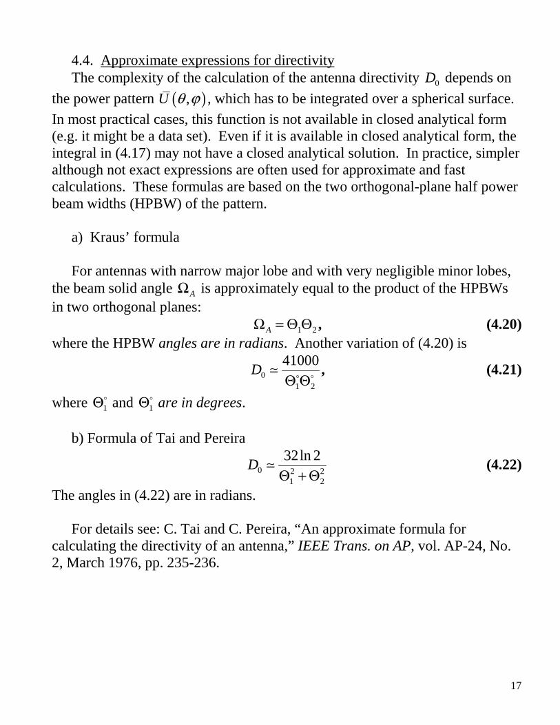
The effective antenna aperture is the ratio of the available powerat the terminals of the antenna to the power flux density of a planewave incident upon the antenna, which is polarization matched tothe antenna. If there is no specific direction chosen, the directionof maximum radiation intensity is implied.

( )1/ 22

20

1/ 2

1/ 2

cos ,2hf hf

I zP R d

lπξ ξ ξ

−

= ⋅ ⋅ =∫

Since the loss resistance lR is defined through the loss power as

20

12hf lP R I= ,

one obtains that:

00.5 0.5 0.349l hf

l fR R

P

π µσ

= ⋅ = = Ω

The antenna efficiency is:73

0.995273 0.349

r

r l

Re

R R= = =

+ +[dB] 1010log 0.9952 0.02e = = −

10. Effective area (aperture) Ae

Ae

i

PA

W= , (4.56)

where:

eA is the effective aperture, m2

AP is the power delivered from the antenna to the load, W

iW is the power flux density (Poynting vector magnitude) of the incidentwave, W/m2

29

Using the Thevenin equivalent of a receiving antenna, one can show thatequation (4.56) relates the antenna impedance and its effective aperture:

( ) ( )2 2

2 2

| | / 2 | |2

A L A Le

i i r l L A L

I R V RA

W W R R R X X= =

+ + + +(4.57)

Under conditions of conjugate matching:

( )2| | 1

8

A L

Ae

i r l

R R

VA

W R R=

=+

(4.58)

For aperture-type antennas, the effective area is smaller than the physicalaperture area. Aperture antennas with constant amplitude and phasedistribution across the aperture have the maximum effective area, which ispractically equal to the geometrical area. The effective aperture of wireantennas is much larger than the surface of the wire itself. Sometimes, theaperture efficiency of an antenna is estimated as the ratio of the effectiveantenna aperture and its physical area:

eap

p

A

Aε = (4.59)

Example: A uniform plane wave is incident upon a very short dipole. Find the

effective area eA assuming that the radiation resistance is2

80l

Rπλ

=

, and

that the field is linearly polarized along the axis of the dipole. Compare eAwith the physical surface of the wire, if / 50l λ= and / 300d λ= , where d isthe wire’s diameter.

Since the dipole is very short, one can neglect the conduction losses.Wire antennas do not have dielectric losses. Therefore, 0lR = . Underconjugate matching (which is implied unless specified otherwise)

2| |8

Ae

i r

VA

W R=

The dipole is very short and one can assume that the E -field intensity isthe same along the whole wire. Then, the voltage created by the inducedelectromotive force of the incident wave is:

| |AV E l= ⋅

30

The Poynting vector has a magnitude of2| |

2i

EW

η= . Then,

2 2 22

2

| | 2 30.119

8 | | 8er

E lA

E R

η λ λπ

⋅ ⋅= = = ⋅⋅ ⋅

The physical surface of the dipole is:2

4 2 6 210 8.7 104 36p

dA

π π λ λ− −= = = × ⋅

The aperture efficiency of this dipole would then be:4

6

0.1191.37 10

8.7 10e

app

A

Aε −= = = ×

×

11. Relation between the directivity 0D and the effective aperture eAThe simplest derivation of this relation goes through two stages.

Stage 1: Prove that the ratio 0 / eD A is the same for any antenna.Consider two antennas: A1 and A2. Let, first, A1 be the transmitting

antenna, and A2 be the receiving one. Let the distance between the twoantennas be R. The power density generated by A1 at A2 is:

1 11 24

D PW

Rπ=

Here, 1P is the total power radiated by A1, and 1D is the directivity of A1.The power received by A2 and delivered to its load is:

2

2

1 11 2 1 24

ee

D P AP A W

Rπ→ = ⋅ = ,

where2eA is the effective area of A2.

2

2 1 21

1

4e

PD A R

Pπ →⇒ =

Now, let A1 be the receiving antenna and A2 be the transmitting one. Onecan derive the following:

1

2 2 12

2

4e

PD A R

Pπ →=

31

If 1 2P P= , then, according to the reciprocity principle in electromagnetics♣,

1 2 2 1P P→ →= . Therefore,

2 1

1 2

1 2

1 2

e e

e e

D A D A

D D

A Aγ

=

⇒ = =

γ is the same for every antenna.

Stage 2: Find the ratio 0 / eD Aγ = for an infinitesimal dipole.

The directivity of a very short dipole (infinitesimal dipole) is 0 1.5idD =(see Examples of Section 4, this Lecture).

The effective aperture of an infinitesimal dipole is 238

ideA λ

π= (see the

Example of Section 10, this Lecture).

02

1.58

3e

D

Aγ π

λ= = ⋅

02

4

e

D

A

πγλ

= = (4.60)

Equation (4.60) assumes that there are no heat losses in the antenna, nopolarization mismatch and no impedance mismatch with the transmissionlines/load. If those factors are present, then:

( )

( )

22 2

0

22 2

0

ˆ ˆ1 | | | |4

ˆ ˆ1 | | | |4

e w a

e w a

A eD

A G

λρ ρπ

λρ ρπ

= − Γ ⋅

= − Γ ⋅

(4.61)

♣ Reciprocity in antenna theory states that if antenna #1 is a transmitting antenna and antenna #2 is a receiving antenna, then

the ratio of transmitted to received power /tra recP P will not change if antenna #1 becomes the receiving antenna and antenna

#2 becomes the transmitting one.

!