Ant System: Optimization by a Colony of Cooperating Agents

IEEE TRANSACTIONS ON SYSTEMS, MAN, AND CYBERNETICS-PART B CYBERNETICS, VOL 26, NO 1, FEBRUARY 1996

Ant System: Optimization by a Colony of Cooperating Agents

Marco Dorigo, Member, ZEEE, Vittorio Maniezzo, and Albert0 Colorni

29

Abstract-An analogy with the way ant colonies function has suggested the definition of a new computational paradigm, which we call Ant System. We propose it as a viable new approach to stochastic combinatorial optimization. The main characteristics of this model are positive feedback, distributed computation, and the use of a constructive greedy heuristic. Positive feedback accounts for rapid discovery of good solutions, distributed computation avoids premature convergence, and the greedy heuristic helps find acceptable solutions in the early stages of the search process. We apply the proposed methodology to the classical Traveling Salesman Problem (TSP), and report simulation results. We also discuss parameter selection and the early setups of the model, and compare it with tabu search and simulated annealing using TSP. To demonstrate the robustness of the approach, we show how the Ant System (AS) can be applied to other optimization problems like the asymmetric traveling salesman, the quadratic assignment and the job-shop scheduling. Finally we discuss the salient characteristics-global data structure revision, distributed communication and probabilistic transitions of the AS.

I. INTRODUCTION

N this paper we define a new general-purpose heuristic al- I gorithm which can be used to solve different combinatorial optimization problems. The new heuristic has the following desirable characteristics:

It is versatile, in that it can be applied to similar versions of the same problem; for example, there is a straightforward extension from the traveling salesman problem (TSP) to the asymmetric traveling salesman problem (ATSP). It is robust. It can be applied with only minimal changes to other combinatorial optimization problems such as the quadratic assignment problem (QAP) and the job-shop scheduling problem (JSP). It is a population based approach. This is interesting because it allows the exploitation of positive feedback as a search mechanism, as explained later in the paper. It also

Manuscript received November 15, 1991; revised September 3, 1993, July 2, 1994, and December 28, 1994.

M. Dorigo was with the Progetto di Intelligenza Artificiale e Robot- ica, Dipartimento di Elettronica e Informazione, Politecnico di Mi- lano, 20133 Milano, Italy. He is now with INDIA, Universite’ Libre de Bruxelles, 1050 Bruxelles, Belgium (e-mail: [email protected], http://iridia.ulb.ac. be/dorigo/dorigo.html).

V. Maniezzo was with the Progetto di Intelligenza Artificiale e Robotica, Dipartimento di Elettronica e Informazione, Politecnico di Milano, 20133 Milano, Italy. He is now with Dipartimento di Scienze dell’Informazione, Universita’ di Bologna, 47023 Cesena, Italy (e-mail: [email protected], http://www.csr.unibo.it/-maniezzo).

A. Colorni is with the Dipartimento di Elettronica e Informazione, Politecnico di Milano, 20133 Milano, Italy (e-mail: [email protected]).

Publisher Item Identifier S 1083-4419(96)00417-7

makes the system amenable to parallel implementations (though this is not considered in this paper).

These desirable properties are counterbalanced by the fact that, for some applications, the Ant System can be outperformed by more specialized algorithms. This is a problem shared by other popular approaches like simulated annealing (SA), and tabu search (TS), with which we compare the Ant System. Nevertheless, we believe that, as is the case with SA and TS, our approach is meaningful in view of applications to problems which, although very similar to well known and studied basic problems, present peculiarities which make the application of the standard best-performing algorithm impossible. This is the case, for example, with the ATSP.

In the approach discussed in this paper we distribute the search activities over so-called “ants,” that is, agents with very simple basic capabilities which, to some extent, mimic the behavior of real ants. In fact, research on the behavior of real ants has greatly inspired our work (see [lo], [ll], [21]). One of the problems studied by ethologists was to understand how almost blind animals like ants could manage to establish shortest route paths from their colony to feeding sources and back. It was found that the medium used to communicate information among individuals regarding paths, and used to decide where to go, consists of pheromone trails. A moving ant lays some pheromone (in varying quantities) on the ground, thus marking the path by a trail of this substance. While an isolated ant moves essentially at random, an ant encountering a previously laid trail can detect it and decide with high probability to follow it, thus reinforcing the trail with its own pheromone. The collective behavior that emerges is a form of autocatalytic behavior’ where the more the ants following a trail, the more attractive that trail becomes for being followed. The process is thus characterized by a positive feedback loop, where the probability with which an ant chooses a path increases with the number of ants that previously chose the same path.

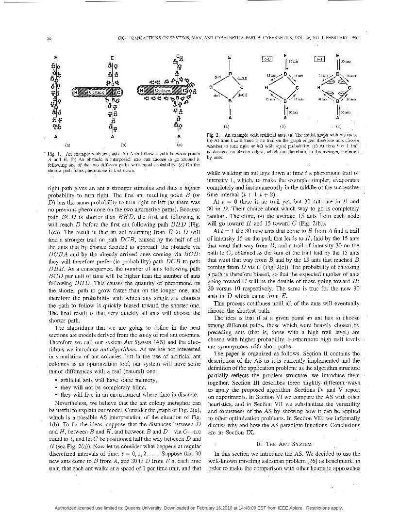
Consider for example the experimental setting shown in Fig. 1. There is a path along which ants are walking (for example from food source A to the nest E , and vice versa, see Fig. l(a)). Suddenly an obstacle appears and the path is cut off. So at position B the ants walking from A to E (or at position D those walking in the opposite direction) have to decide whether to turn right or left (Fig. l(b)). The choice is influenced by the intensity of the pheromone trails left by preceding ants. A higher level of pheromone on the

‘An autocatalytic [12], i.e. positive feedback, process is a process that reinforces itself, in a way that causes very rapid convergence and, if no limitation mechanism exists, leads to explosion.

10834419/96$05.00 0 1996 IEEE

Authorized licensed use limited to: Queens University. Downloaded on February 16,2010 at 14:48:09 EST from IEEE Xplore. Restrictions apply.

http://iridia.ulb.ac

http://www.csr.unibo.it/-maniezzo

30

E

A

E

&I8 8 8

IEEE TRANSACTIONS ON SYSTEMS. MAN, AND CYBERNETICS-PART B: CYBERNETICS, VOL. 26, NO. 1, FEBRUARY 1996

i

f A f A

(a) (b) (c) Fig. 1. An example with real ants. (a) Ants follow a path between points A and E. (b) An obstacle is interposed; ants can choose to go around it following one of the two different paths with equal probability. (c) On the shorter path more pheromone is laid down.

right path gives an ant a stronger stimulus and thus a higher probability to turn right. The first ant reaching point B (or D ) has the same probability to turn right or left (as there was no previous pheromone on the two alternative paths). Because path B C D is shorter than B H D , the first ant following it will reach D before the first ant following path B H D (Fig. l(c)). The result is that an ant returning from E to D will find a stronger trail on path D C B , caused by the half of all the ants that by chance decided to approach the obstacle via D C B A and by the already arrived ones coming via BCD: they will therefore prefer (in probability) path D C B to path D H B . As a consequence, the number of ants following path BCD per unit of time will be higher than the number of ants following E H D . This causes the quantity of pheromone on the shorter path to grow faster than on the longer one, and therefore the probability with which any single ant chooses the path to follow is quickly biased toward the shorter one. The final result is that very quickly all ants will choose the shorter path.

The algorithms that we are going to define in the next sections are models derived from the study of real ant colonies. Therefore we call our system Ant System (AS) and the algorithms we introduce ant algorithms. As we are not interested in simulation of ant colonies, but in the use of artificial ant colonies as an optimization tool, our system will have some major differences with a real (natural) one:

e artificial ants will have some memory, 0 they will not be completely blind, 0 they will live in an environment where time is discrete. Nevertheless, we believe that the ant colony metaphor can

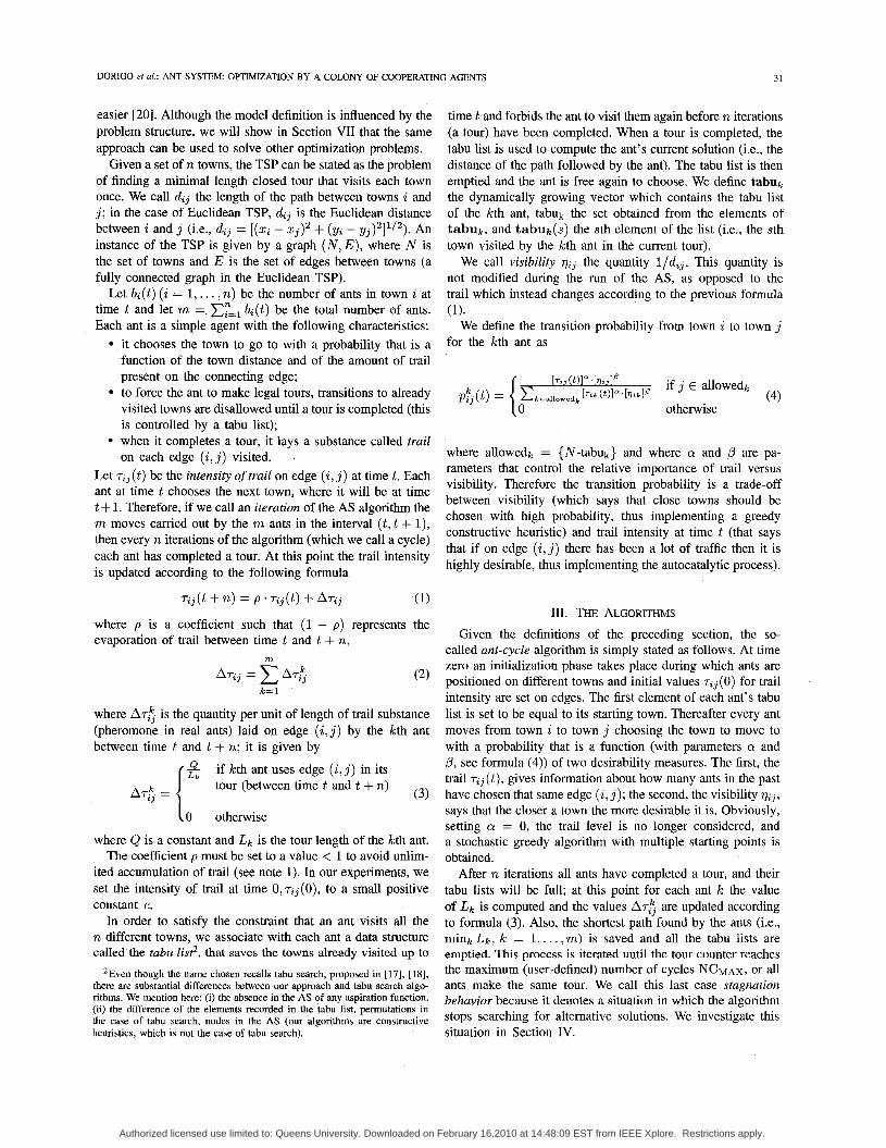
be useful to explain our model. Consider the graph of Fig. 2(a), which is a possible AS interpretation of the situation of Fig. l(b). To fix the ideas, suppose that the distances between D and H , between B and H , and between B and D-via C-are equal to 1, and let C be positioned half the way between D and B (see Fig. 2(a)). Now let us consider what happens at regular discretized intervals of time: t = 0 , 1 , 2 , new ants come to B from A , and 30 to D from E at each time unit, that each ant walks at a speed of 1 per time unit, and that

I A

(a)

I A

Fig. 2. An example with artificial ants. (a) The initial graph with distances. @) At time t = 0 there is no trail on the graph edges; therefore ants choose whether to turn right or left with equal probability. (c) At time t = 1 trail is stronger on shorter edges, which are therefore, in the average, preferred by ants.

while walking an ant lays down at time t a pheromone trail of intensity 1, which, to make the example simpler, evaporates completely and instantaneously in the middle of the successive time interval (t + 1, t + 2).

At t = 0 there is no trail yet, but 30 ants are in B and 30 in D. Their choice about which way to go is completely random. Therefore, on the average 15 ants from each node will go toward H and 15 toward C (Fig. 2(b)).

At t = 1 the 30 new ants that come to B from A find a trail of intensity 15 on the path that leads to H , laid by the 15 ants that went that way from E, and a trail of intensity 30 on the path to C, obtained as the sum of the trail laid by the 15 ants that went that way from B and by the 15 ants that reached B coming from D via C (Fig. 2(c)). The probability of choosing a path is therefore biased, so that the expected number of ants going toward C will be the double of those going toward H : 20 versus 10 respectively. The same is true for the new 30 ants in D which came from E.

This process continues until all of the ants will eventually choose the shortest path.

The idea is that if at a given point an ant has to choose among different paths, those which were heavily chosen by preceding ants (that is, those with a high trail level) are chosen with higher probability. Furthermore high trail levels are synonymous with short paths.

The paper is organized as follows. Section I1 contains the description of the AS as it is currently implemented and the definition of the application problem: as the algorithm structure partially reflects the problem structure, we introduce them together. Section I11 describes three slightly different ways to apply the proposed algorithm. Sections IV and V report on experiments. In Section VI we compare the AS with other heuristics, and in Section VI1 we substantiate the versatility and robustness of the AS by showing how it can be applied to other optimization problems. In Section VI11 we informally discuss why and how the AS paradigm functions. Conclusions are in Section IX.

11. THE ANT SYSTEM

In this section we introduce the AS. We decided to use the well-known traveling salesman problem [26] as benchmark, in order to make the comparison with other heuristic approaches


DORIGO et al.: ANT SYSTEM OPTIMIZATION BY A COLONY OF COOPERATING AGENTS 31

easier [2O]. Although the model definition is influenced by the problem structure, we will show in Section VI1 that the same approach can be used to solve other optimization problems.

Given a set of n towns, the TSP can be stated as the problem of finding a minimal length closed tour that visits each town once. We call d,, the length of the path between towns i and j ; in the case of Euclidean TSP, di, is the Euclidean distance between i and j (i.e., d,, = [(z, - 2,)' + (y, - TJ,)']~/'). An instance of the TSP is given by a graph ( N , E ) , where N is the set of towns and E is the set of edges between towns (a fully connected graph in the Euclidean TSP).

Let b,(t) (i = 1, . . . , n) be the number of ants in town i at time t and let m = b,(t) be the total number of ants. Each ant is a simple agent with the following characteristics:

it chooses the town to go to with a probability that is a function of the town distance and of the amount of trail present on the connecting edge; to force the ant to make legal tours, transitions to already visited towns are disallowed until a tour is completed (this is controlled by a tabu list); when it completes a tour, it lays a substance called trail on each edge ( i , j ) visited.

Let r,, ( t ) be the intensity of trail on edge (i, j ) at time t. Each ant at time t chooses the next town, where it will be at time t + 1. Therefore, if we call an iteration of the AS algorithm the m moves carried out by the m ants in the interval ( t , t + l), then every n iterations of the algorithm (which we call a cycle) each ant has completed a tour. At this point the trail intensity is updated according to the following formula

(1)

where p is a coefficient such that (1 - p ) represents the evaporation of trail between time t and t + n,

Tz, (t + n) = p . T,, (t) + AT,,

m

k=l

where AT$ is the quantity per unit of length of trail substance (pheromone in real ants) laid on edge ( i , j ) by the kth ant between time t and t + n; it is given by

E if kth ant uses edge ( i , j ) in its tour (between time t and t + n)

( 3 ) = 8 ,

l o otherwise

where Q is a constant and Lk is the tour length of the kth ant. The coefficient p must be set to a value < 1 to avoid unlim-

ited accumulation of trail (see note 1). In our experiments, we set the intensity of trail at time O , r i j ( O ) , to a small positive constant c.

In order to satisfy the constraint that an ant visits all the n different towns, we associate with each ant a data structure called the tabu lis$, that saves the towns already visited up to

'Even though the name chosen recalls tabu search, proposed in [17], [18], there are substantial differences between our approach and tabu search algorithms. We mention here: (i) the absence in the AS of any aspiration function, (ii) the difference of the elements recorded in the tabu list, permutations in the case of tabu search, nodes in the AS (our algorithms are constructive heuristics, which is not the case of tabu search).

time t and forbids the ant to visit them again before n iterations (a tour) have been completed. When a tour is completed, the tabu list is used to compute the ant's current solution (i.e., the distance of the path followed by the ant). The tabu list is then emptied and the ant is free again to choose. We define tabuk the dynamically growing vector which contains the tabu list of the kth ant, tabUk the set obtained from the elements of tabuk, and tabuk(s) the sth element of the list (i.e., the sth town visited by the kth ant in the current tour).

We call visibility q;j the quantity l /di j . This quantity is not modified during the run of the AS, as opposed to the trail which instead changes according to the previous formula (1).

We define the transition probability from town i to town j for the kth ant as

where allowedk = {N-tabuk} and where a and p are parameters that control the relative importance of trail versus visibility. Therefore the transition probability is a trade-off between visibility (which says that close towns should be chosen with high probability, thus implementing a greedy constructive heuristic) and trail intensity at time t (that says that if on edge (i,j) there has been a lot of traffic then it is highly desirable, thus implementing the autocatalytic process).

111. THE ALGORITHMS

Given the definitions of the preceding section, the so- called ant-cycle algorithm is simply stated as follows. At time zero an initialization phase takes place during which ants are positioned on different towns and initial values rz, (0) for trail intensity are set on edges. The first element of each ant's tabu list is set to be equal to its starting town. Thereafter every ant moves from town i to town j choosing the town to move to with a probability that is a function (with parameters a and p, see formula (4)) of two desirability measures. The first, the trail T,, ( t ) , gives information about how many ants in the past have chosen that same edge (i, j ) ; the second, the visibility q,,, says that the closer a town the more desirable it is. Obviously, setting a = 0, the trail level is no longer considered, and a stochastic greedy algorithm with multiple starting points is obtained.

After n iterations all ants have completed a tour, and their tabu lists will be full; at this point for each ant k the value of Lk is computed and the values Ar; are updated according to formula (3) . Also, the shortest path found by the ants (i.e., mink Lk, k = 1, . . . , m) is saved and all the tabu lists are emptied. This process is iterated until the tour counter reaches the maximum (user-defined) number of cycles NCMAX, or all ants make the same tour. We call this last case stagnation behavior because it denotes a situation in which the algorithm stops searching for alternative solutions. We investigate this situation in Section IV.


32 IEEE TRANSACTIONS ON SYSTEMS, MAN, AND CYBERNETICS-PART B CYBERNETICS, VOL 26, NO 1, FEBRUARY 1996

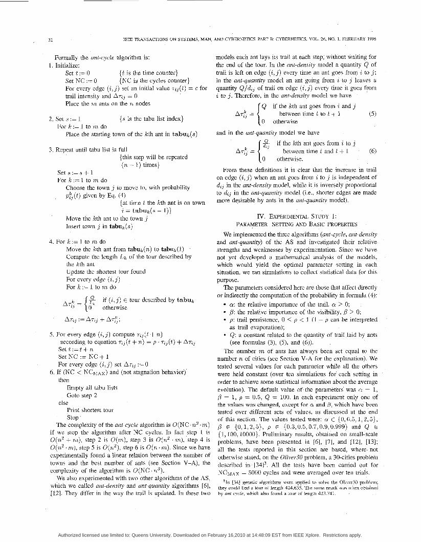
Formally the ant-cycle algorithm is: 1. Initialize:

Set t := 0 Set NC := 0 For every edge (i,j) set an initial value ri3(t) = c for trail intensity and ArZ3 = 0 Place the m ants on the n nodes

{t is the time counter} {NC is the cycles counter}

2. Set s := 1 { s is the tabu list index} For k := 1 to m do

Place the starting town of the kth ant in tabuk(s)

3. Repeat until tabu list is full {this step will be repeated (n - 1) times}

Set s := s + 1 For k := 1 to m do

Choose the town j to move to, with probability P:j ( t ) given by Eq. (4)

{at time t the kth ant is on town i = tabuk(s - 1))

Move the kth ant to the town j Insert town j in tabuk(s)

4. For k := 1 to m do Move the kth ant from tabuk(n) to tabuk(1) Compute the length LI, of the tour described by the kth ant Update the shortest tour found For every edge ( i , j ) For k : = 1 to m do

E 0 otherwise

if (i,j) E tour described by tabuk

5. For every edge ( 2 , j ) compute rZ3 (t + n) according to equation rZj(t + n) = p . r,,(t) + Arz3

Set t : = t + n Set NC := NC + 1 For every edge (i, j ) set ArZj := 0

then 6. If (NC < NCMAX) and (not stagnation behavior)

Empty all tabu lists Goto step 2

Print shortest tour else

stop The complexity of the ant-cycle algorithm i s O(NC.n2 .rn)

if we stop the algorithm after NC cycles. In fact step 1 is O(n2 + m), step 2 is O(rn), step 3 i s O(n2 . m), step 4 is O(n2 .m), step 5 is O(n2) , step 6 is O(n.rn). Since we have experimentally found a linear relation between the number of towns and the best number of ants (see Section V-A), the complexity of the algorithm is O(NC . n3).

We also experimented with two other algorithms of the AS, which we called ant-density and ant-quantity algorithms [6], [12]. They differ in the way the trail is updated. In these two

models each ant lays its trail at each step, without waiting for the end of the tour. In the ant-density model a quantity Q of trail is left on edge ( i , j ) every time an ant goes from i to j ; in the ant-quantity model an ant going from i to j leaves a quantity Q/d,, of trail on edge (i,j) every time it goes from i to j . Therefore, in the ant-density model we have

Q

0 otherwise

if the kth ant goes from i and j between time t to t + 1 (5)

if the kth ant goes from i to j between time t and t + 1

{ AI-; =

and in the ant-quantity model we have

(6) 0 otherwise.

From these definitions it is clear that the increase in trail on edge (i,j) when an ant goes from z to j is independent of dZ, in the ant-density model, while it is inversely proportional to d,, in the ant-quantity model (i.e., shorter edges are made more desirable by ants in the ant-quantity model).

IV. EXPERIMENTAL STUDY 1: PARAMETER SE'ITING AND BASIC PROPERTIES

We implemented the three algorithms (ant-cycle, ant-density and ant-quantity) of the AS and investigated their relative strengths and weaknesses by experimentation. Since we have not yet developed a mathematical analysis of the models, which would yield the optimal parameter setting in each situation, we ran simulations to collect statistical data for this purpose.

The parameters considered here are those that affect directly or indirectly the computation of the probability in formula (4):

a: the relative importance of the trail, a! 2 0; 0 ,B: the relative importance of the visibility, /3 2 0;

p: trail persistence, 0 5 p < 1 (1 - p can be interpreted

* Q: a constant related to the quantity of trail laid by ants as trail evaporation);

(see formulas (3), (3, and (6)). The number m of ants has always been set equal to the

number n of cities (see Section V-A for the explanation). We tested several values for each parameter while all the others were held constant (over ten simulations for each setting in order to achieve some statistical information about the average evolution). The default value of the parameters was a! = 1, p = 1, p = 0.5, Q = 100. In each experiment only one of the values was changed, except for a and ,B, which have been tested over different sets of values, as discussed at the end of this section. The values tested were: a: E {0,0.5,1,2,5}, ,O E {0,1,2,5}, p E (0.3,0.5,0.7,0.9,0.999} and Q E {I, 100, lOOOO}. Preliminary results, obtained on small-scale problems, have been presented in [ 6 ] , [7], and [12], [13]; all the tests reported in this section are based, where not otherwise stated, on the Oliver30 problem, a 30-cities problem described in [3413. All the tests have been carried out for N C M A ~ = 5000 cycles and were averaged over ten trials.

31n [34] genetic algorithms were applied to solve the Oliver30 problem; they could find a tour of length 424.635. The same result was often obtained by ant-cycle, which also found a tour of length 423.741.


DORIGO et al.: ANT SYSTEM: OPTIMIZATION BY A COLONY OF COOPERATINI

ant-density

ant-quantity

ant-cycle

TABLE I COMPARISON AMONG ANT-QUANTITY, ANT-DENSITY,

AND ANT-CYCLE. AVERAGES OVER 10 TRIALS

Best parameter set Average result Best result

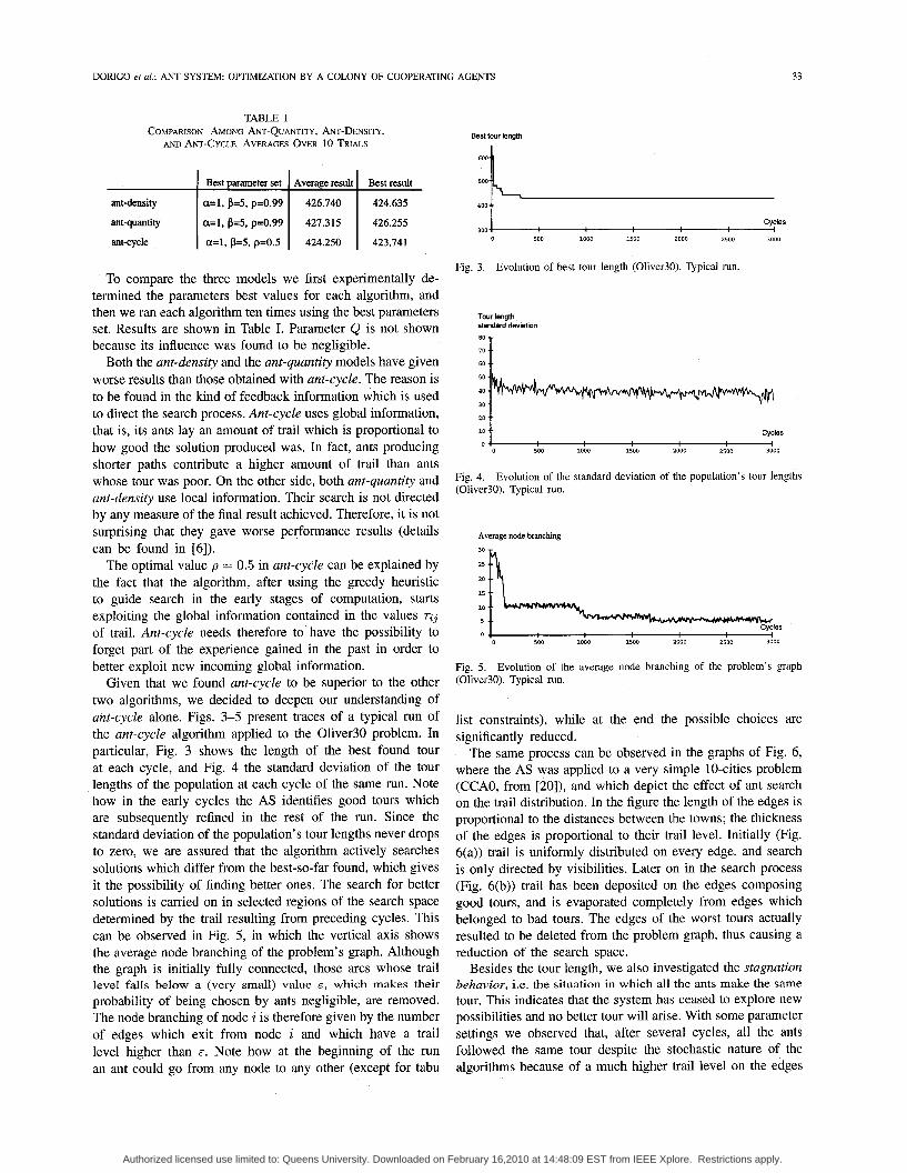
a=l, p=5, pO.99 426.740 424.635

a=l, p=5, p0.99 427.315 426.255

a=l, p=5, p 0 . 5 424.250 423.741

To compare the three models we first experimentally determined the parameters best values for each algorithm, and then we ran each algorithm ten times using the best parameters set. Results are shown in Table I. Parameter Q is not shown because its influence was found to be negligible.

Both the ant-density and the ant-quantity models have given worse results than those obtained with ant-cycle. The reason is to be found in the kind of feedback information which is used to direct the search process. Ant-cycle uses global information, that is, its ants lay an amount of trail which is proportional to how good the solution produced was. In fact, ants producing shorter paths contribute a higher amount of trail than ants whose tour was poor. On the other side, both ant-quantity and ant-density use local information. Their search is not directed by any measure of the final result achieved. Therefore, it is not surprising that they gave worse performance results (details can be found in [6]).

The optimal value p = 0.5 in ant-cycle can be explained by the fact that the algorithm, after using the greedy heuristic to guide search in the early stages of computation, starts exploiting the global information contained in the values rt3 of trail. Ant-cycle needs therefore to have the possibility to forget part of the experience gained in the past in order to better exploit new incoming global information.

Given that we found ant-cycle to be superior to the other two algorithms, we decided to deepen our understanding of ant-cycle alone. Figs. 3-5 present traces of a typical run of the ant-cycle algorithm applied to the Oliver30 problem. In particular, Fig. 3 shows the length of the best found tour at each cycle, and Fig. 4 the standard deviation of the tour lengths of the population at each cycle of the same run. Note how in the early cycles the AS identifies good tours which are subsequently refined in the rest of the run. Since the standard deviation of the population’s tour lengths never drops to zero, we are assured that the algorithm actively searches solutions which differ from the best-so-far found, which gives it the possibility of finding better ones. The search for better solutions is carried on in selected regions of the search space determined by the trail resulting from preceding cycles. This can be observed in Fig. 5, in which the vertical axis shows the average node branching of the problem’s graph. Although the graph is initially fully connected, those arcs whose trail level falls below a (very small) value E , which makes their probability of being chosen by ants negligible, are removed. The node branching of node i is therefore given by the number of edges which exit from node i and which have a trail level higher than E . Note how at the beginning of the run an ant could go from any node to any other (except for tabu

3 AGENTS 33

Best lour length

400

Cycles 300 I

0 500 1000 1500 2000 2500 3000

Fig. 3. Evolution of best tour length (Oliver30). Typical run.

Tour lenglh standard deviation

60

Cycles

0 500 lob0 li00 aooo 2500 3000 _ .

Fig. 4. (Oliver30). Typical run.

Evolution of the standard deviation of the population’s tour lengths

Average no& branching

5 - - Cycles

0 500 1000 1500 2000 2500 3000 0 - I

Fig. 5. (Oliver30). Typical run.

Evolution of the average node branching of the problem’s graph

list constraints), while at the end the possible choices are significantly reduced.

The same process can be observed in the graphs of Fig. 6, where the AS was applied to a very simple 10-cities problem (CCAO, from [20]), and which depict the effect of ant search on the trail distribution. In the figure the length of the edges is proportional to the distances between the towns; the thickness of the edges is proportional to their trail level. Initially (Fig. 6(a)) trail is uniformly distributed on every edge, and search is only directed by visibilities. Later on in the search process (Fig. 6(b)) trail has been deposited on the edges composing good tours, and is evaporated completely from edges which belonged to bad tours. The edges of the worst tours actually resulted to be deleted from the problem graph, thus causing a reduction of the search space.

Besides the tour length, we also investigated the stagnation behnvior, i.e. the situation in which all the ants make the same tour. This indicates that the system has ceased to explore new possibilities and no better tour will arise. With some parameter settings we observed that, after several cycles, all the ants followed the same tour despite the stochastic nature of the algorithms because of a much higher trail level on the edges


34 IEEE TRANSACTIONS ON SYSTEMS, MAN, AND CYBERNETICS-PART B. CYBERNETICS, VOL. 26, NO. 1, FEBRUARY 1996

10

3 5

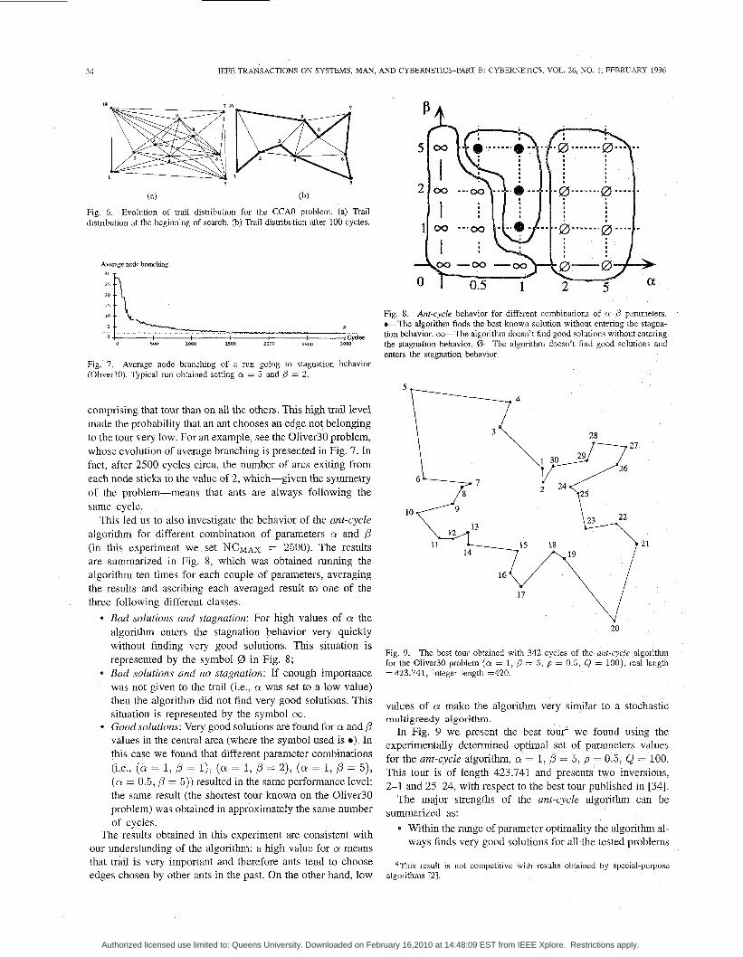
(a) CD) Fig. 6. Evolution of trail distribution for the CCAO problem. (a) Trail distribution at the beginning of search. (b) Trail distribution after 100 cycles.

Average node branching

15 .. 10

5

- - Fig. 8. Ant-cycle behavior for different combinations of C Y - ~ parameters. *-The algorithm finds the best known solution without entering the stagnation behavior. oo-The algorithm doesn’t find good solutions without entering

0 500 1000 1500 2000 2500 3000 the stagnation behavior. @-The algorithm doesn’t find good solutions and

.- 2 , ..... 0 - ..... . ................................... ........... _..

enters the stagnation behavior. Fig. 7. (Oliver30). Typical run obtained setting cy = 5 and p = 2.

Average node branching of a rnn going to stagnation behavior

comprising that tour than on all the others. This high trail level made the probability that an ant chooses an edge not belonging to the tour very low. For an example, see the Oliver30 problem, whose evolution of average branching is presented in Fig. 7. In fact, after 2500 cycles circa, the number of arcs exiting from each node sticks to the value of 2, which-given the symmetry of the problem-means that ants are always following the same cycle.

This led us to also investigate the behavior of the ant-cycle algorithm for different combination of parameters a and p (in this experiment we set N C M A ~ = 2500). The results are summarized in Fig. 8, which was obtained running the algorithm ten times for each couple of parameters, averaging the results and ascribing each averaged result to one of the three following different classes.

0 Bad solutions and stagnation: For high values of a the

without finding very good solutions. This situation is

* Bad solutions and no stagnation: If enough importance was not given to the trail (i.e., Q was set to a low value)

algorithm enters the stagnation behavior very quickly 20

Fig. 9. The best tour obtained with 342 cycles of the ant-cycle algorithm for the Oliver30 problem (CY = 1, p = 5 , p = 0.5, Q = loo) , real length =423.741, integer length =420.

represented by the symbol 0 in Fig. 8;

then the algorithm did not find very good solutions. This situation is represented by the symbol 00.

0 Good solutions: Very good solutions are found for a and p values in the central area (where the symbol used is 0) . In this case we found that different parameter combinations ( i . e . , ( Q = l , p = l ) , ( a ! = l , P = 2 ) , ( a : = l , p = 5 } , (a = 0.5, p = 5)) resulted in the same performance level: the same result (the shortest tour known on the Oliver30 problem) was obtained in approximately the same number

values of a! make the algorithm very similar to a stochastic multigreedy algorithm.

In Fig. 9 we present the best tour4 we found using the experimentally determined optimal set of parameters values for the ant-cycle algorithm, a! = 1, /3 = 5, p = 0.5, Q = 100. This tour is of length 423.741 and presents two inversions, 2-1 and 25-24, with respect to the best tour published in [34].

The major strengths of the ant-cycle algorithm can be summarized as:

0 Within the range of parameter optimality the algorithm always finds very good solutions for all the tested problems

of cycles. The results obtained in this experiment are consistent with

our understanding of the algoritha: a high value for a means that is very important and therefore ants tend to choose 4 T h ~ s result is not competitive with results obtamed by special-purpose edges chosen by other ants in the past. On the other hand, low algorithms [2]


DORIGO et al.: ANT SYSTEM: OPTIMIZATION BY A COLONY OF COOPERATING AGENTS 35

Best tour length

400 t Cycles 10

0-0 1 I ri 0

O- T g T-T 0 -0 T 300 ! I I I

8

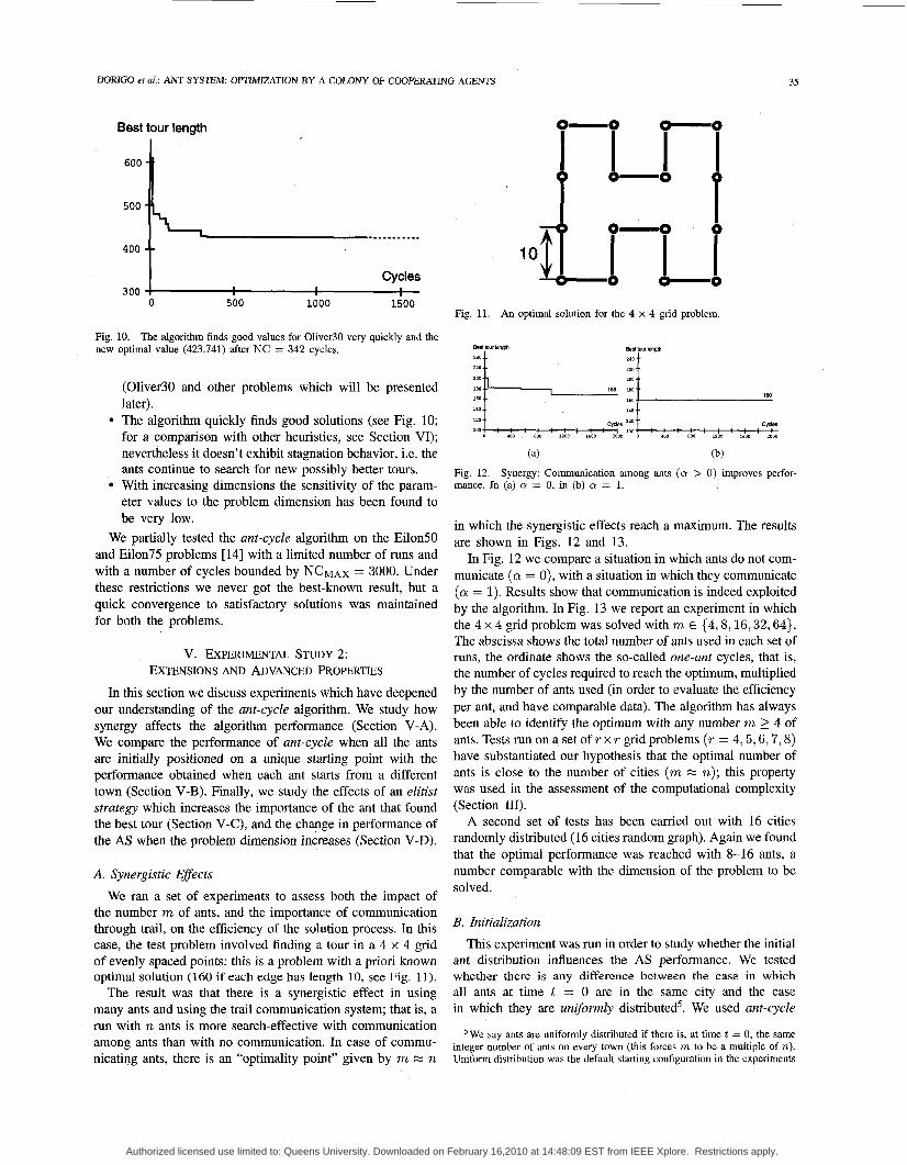
0 500 1000 1500 Fig. 11. An optimal solution for the 4 x 4 grid problem.

Fig. 10. new optimal value (423.741) after NC = 342 cycles.

The algorithm finds good values for Oliver30 very quickly and the

(Oliver30 and other problems which will be presented later). The algorithm quickly finds good solutions (see Fig. 10; for a comparison with other heuristics, see Section VI); nevertheless it doesn’t exhibit stagnation behavior, i.e. the ants continue to search for new possibly better tours. With increasing dimensions the sensitivity of the parameter values to the problem dimension has been found to be very low.

We partially tested the ant-cycle algorithm on the EilonSO and Eilon75 problems [ 141 with a limited number of runs and with a number of cycles bounded by N C M A ~ = 3000. Under these restrictions we never got the best-known result, but a quick convergence to satisfactory solutions was maintained for both the problems.

V. EXPERIMENTAL STUDY 2: EXTENSIONS AND ADVANCED PROPERTIES

In this section we discuss experiments which have deepened our understanding of the ant-cycle algorithm. We study how synergy affects the algorithm performance (Section V-A). We compare the performance of ant-cycle when all the ants are initially positioned on a unique starting point with the performance obtained when each ant starts from a different town (Section V-B). Finally, we study the effects of an elitist strategy which increases the importance of the ant that found the best tour (Section V-C), and the change in performance of the AS when the problem dimension increases (Section V-D).

A. Synergistic Effects

We ran a set of experiments to assess both the impact of the number m of ants, and the importance of communication through trail, on the efficiency of the solution process. In this case, the test problem involved finding a tour in a 4 x 4 grid of evenly spaced points: this is a problem with a priori known optimal solution (160 if each edge has length 10, see Fig. 11).

The result was that there is a synergistic effect in using many ants and using the trail communication system; that is, a

1.0 t 1‘0 +

(a) (b)

Fig. 12. mance. In (a) a = 0, in (b) cy = 1.

Synergy: Communication among ants (a > 0) improves perfor-

in which the synergistic effects reach a maximum. The results are shown in Figs. 12 and 13.

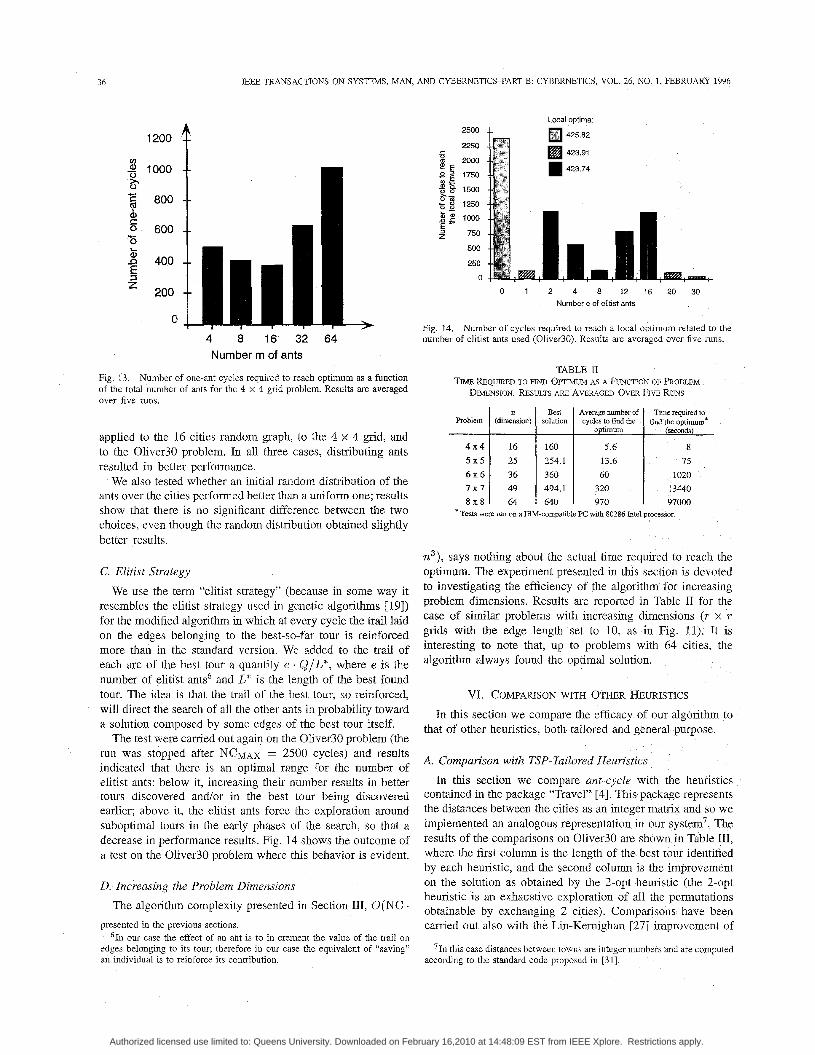
In Fig. 12 we compare a situation in which ants do not communicate ( a = 0), with a situation in which they communicate (a = 1). Results show that communication is indeed exploited by the algorithm. In Fig. 13 we report an experiment in which the 4 x 4 grid problem was solved with m E {4,8,16,32,64}. The abscissa shows the total number of ants used in each set of runs, the ordinate shows the so-called one-ant cycles, that is, the number of cycles required to reach the optimum, multiplied by the number of ants used (in order to evaluate the efficiency per ant, and have comparable data). The algorithm has always been able to identify the optimum with any number m 2 4 of ants. Tests run on a set of T x T grid problems (T = 4,5,6,7,8) have substantiated our hypothesis that the optimal number of ants is close to the number of cities (m M n); this property was used in the assessment of the computational complexity (Section 111).

A second set of tests has been carried out with 16 cities randomly distributed (16 cities random graph). Again we found that the optimal performance was reached with 8-16 ants, a number comparable with the dimension of the problem to be solved.

B. Initialization

This experiment was run in order to study whether the initial ant distribution influences the AS performance. We tested whether there is any difference between the case in which all ants at time t = 0 are in the same city and the case in which they are uniformly distributed5. We used ant-cycle

run with n ants is more search-effective with communication among ants than with no communication. In case of commu-

We say ants are uniformly distributed if there is, at time t = 0, the same inteeer number of ants on every town (this forces m to be a multiple of n).

nicating ants, there is an “optimality point” given by m M n Uniform distribution was the default starting configuration in the experiments


36

hoblem

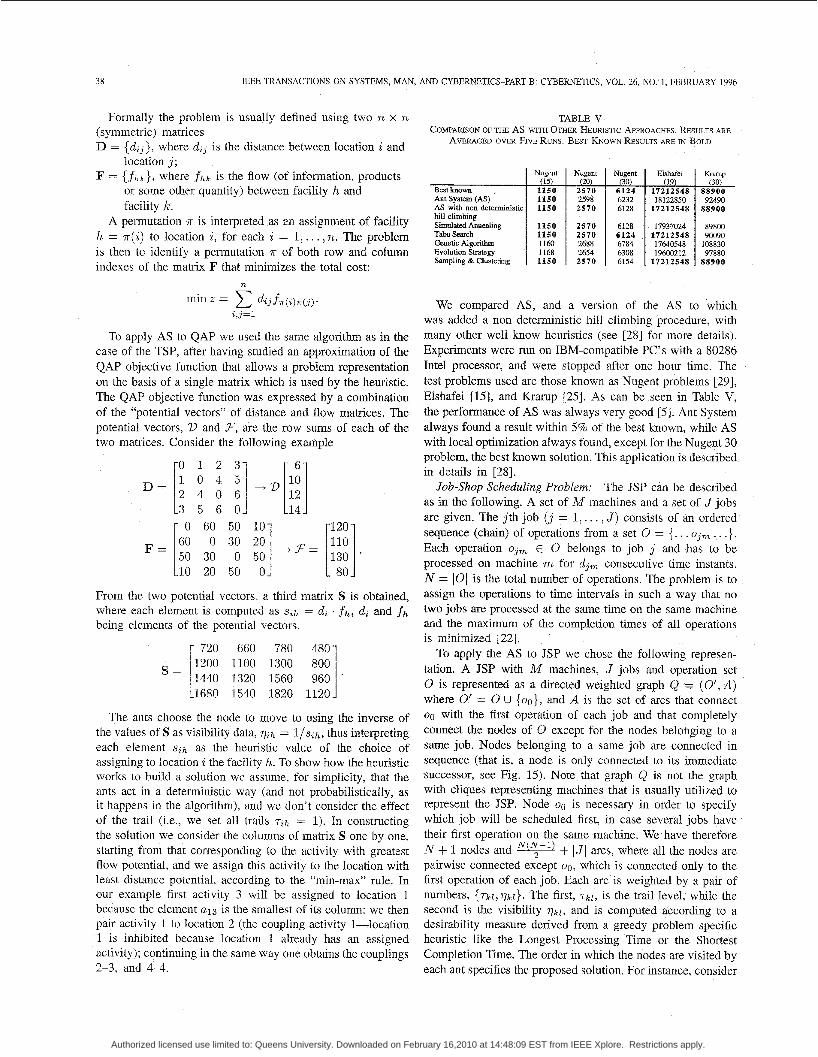
4x4 5 x 5 6 x 6 7 x 7 8 x 8

IEEE TRANSACTIONS ON SYSTEMS, MAN, AND CYBERNETICS-PART B: CYEERNETICS, VOL. 26, NO. 1, FEBRUARY 1996

Best Average number of Time requlred to (dmenslon) solution cycles to find the find the optimum*

optimum (seconds)

16 160 5.6 8 25 254.1 13.6 75 36 360 60 1020 49 494.1 320 13440 64 640 970 97000

1200

(0 -g 1000 6

800

0 600 ”0 ti, n 400

200 z

0

C

5

4 8 16 32 64 Number m of ants

Fig. 13. Number of one-ant cycles required to reach optimum as a function of the total number of ants for the 4 x 4 grid problem. Results are averaged over five runs.

applied to the 16 cities random graph, to the 4 x 4 grid, and to the Oliver30 problem. In all three cases, distributing ants resulted in better performance.

We also tested whether an initial random distribution of the ants over the cities performed better than a uniform one; results show that there is no significant difference between the two choices, even though the random distribution obtained slightly better results.

C. Elitist Strategy

We use the term “elitist strategy” (because in some way it resembles the elitist strategy used in genetic algorithms [19]) for the modified algorithm in which at every cycle the trail laid on the edges belonging to the best-so-far tour is reinforced more than in the standard version. We added to the trail of each arc of the best tour a quantity e . Q/L*, where e is the number of elitist ants6 and L* is the length of the best found tour. The idea is that the trail of the best tour, so reinforced, will direct the search of all the other ants in probability toward a solution composed by some edges of the best tour itself.

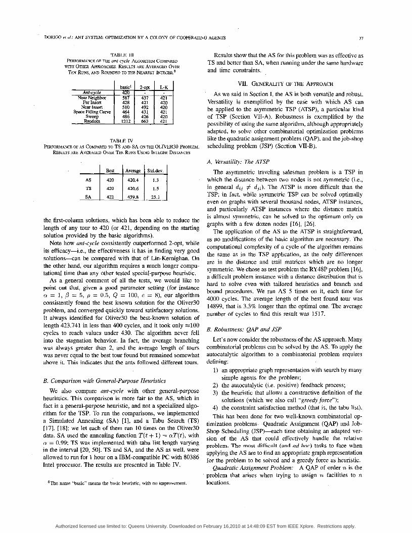
The test were carried out again on the Oliver30 problem (the run was stopped after N C M A ~ = 2500 cycles) and results indicated that there is an optimal range for the number of elitist ants: below it, increasing their number results in better tours discovered andlor in the best tour being discovered earlier; above it, the elitist ants force the exploration around suboptimal tours in the early phases of the search, so that a decrease in performance results. Fig. 14 shows the outcome of a test on the Oliver30 problem where this behavior is evident.

D. Increasing the Problem Dimensions The algorithm complexity presented in Section 111, O(NC.

presented in the previous sections. 61n our case the effect of an ant is to in crement the value of the trail on

edges belonging to its tour; therefore in our case the equivalent of “saving” an individual is to reinforce its contribution.

2500

2250

2000

1750

1500

1250

loo0

750

500

250

0

Local optima:

425.82

423.91

423.74

0 1 2 4 8 12 16 20 30 Number e of elitist ants

Fig. 14. number of elitist ants used (Oliver30). Results are averaged over five runs.

Number of cycles required to reach a local optimum related to the

n3), says nothing about the actual time required to reach the optimum. The experiment presented in this section is devoted to investigating the efficiency of the algorithm for increasing problem dimensions. Results are reported in Table I1 for the case of similar problems with increasing dimensions (T x T

grids with the edge length set to 10, as in Fig. 11). It is interesting to note that, up to problems with 64 cities, the algorithm always found the optimal solution.

VI. COMPARISON WITH OTHER HEURISTICS In this section we compare the efficacy of our algorithm to

that of other heuristics, both tailored and general-purpose.

A. Comparison with TSP-Tailored Heuristics

In this section we compare ant-cycle with the heuristics contained in the package “Travel” [4]. This package represents the distances between the cities as an integer matrix and so we implemented an analogous representation in our system7. The results of the comparisons on Oliver30 are shown in Table 111, where the first column is the length of the best tour identified by each heuristic, and the second column is the improvement on the solution as obtained by the 2-opt heuristic (the 2-opt heuristic is an exhaustive exploration of all the permutations obtainable by exchanging 2 cities). Comparisons have been carried out also with the Lin-Kemighan [27] improvement of

71n this case distances between towns are integer numbers and are computed according to the standard code proposed in [3 11.


DONG0 et al.: ANT SYSTEM OPTIMIZATION BY A COLONY OF COOPERATING AGENTS 31

As TS SA

TABLE In F’ERFORMANCE OF THE ant-cycle ALGORITHM COMPARED

WITH OTHER APPROACHES. RESULTS ARE AVERAGED OVER TEN RUNS, AND ROUNDED TO THE NEAREST INTEGER.8

Best Average Std.dev.

420 420.4 1.3

420 420.6 1.5

422 459.8 25.1

Far Insert Near Insert

Sweep Random

TABLE IV PERFORMANCE OF AS COMPARED TO TS AND SA ON THE OLIVER30 PROBLEM.

RESULTS ARE AVERAGED OVER TEN RUNS USING INTEGER DISTANCES

the first-column solutions, which has been able to reduce the length of any tour to 420 (or 421, depending on the starting solution provided by the basic algorithms).

Note how ant-cycle consistently outperformed 2-opt, while its efficacy-i.e., the effectiveness it has in finding very good solutions--can be compared with that of Lin-Kernighan. On the other hand, our algorithm requires a much longer computational time than any other tested special-purpose heuristic.

As a general comment of all the tests, we would like to point out that, given a good parameter setting (for instance a! = 1, ,B = 5 , p = 0.5, Q = 100, e = 8), our algorithm consistently found the best known solution for the Oliver30 problem, and converged quickly toward satisfactory solutions. It always identified for Oliver30 the best-known solution of length 423.741 in less than 400 cycles, and it took only =lo0 cycles to reach values under 430. The algorithm never fell into the stagnation behavior. In fact, the average branching was always greater than 2, and the average length of tours was never equal to the best tour found but remained somewhat above it. This indicates that the ants followed different tours.

B. Comparison with General-purpose Heuristics

We also compare ant-cycle with other general-purpose heuristics. This comparison is more fair to the AS, which in fact is a general-purpose heuristic, and not a specialized algorithm for the TSP. To run the comparisons, we implemented a Simulated Annealing (SA) [l], and a Tabu Search (TS) [17], [18]; we let each of them run 10 times on the Oliver30 data. SA used the annealing function T(t + 1) = a!T(t), with a = 0.99; TS was implemented with tabu list length varying in the interval [20, 501. TS and SA, and the AS as well, were allowed to run for 1 hour on a IBM-compatible PC with 80386 Intel processor. The results are presented in Table IV.

Results show that the AS for this problem was as effective as TS and better than SA, when running under the same hardware and time constraints.

VII. GENERALITY OF THE APPROACH As we said in Section I, the AS is both versatile and robust.

Versatility is exemplified by the ease with which AS can be applied to the asymmetric TSP (ATSP), a particular kind of TSP (Section VII-A). Robustness is exemplified by the possibility of using the same algorithm, although appropriately adapted, to solve other combinatorial optimization problems like the quadratic assignment problem (QAP), and the job-shop scheduling problem (JSP) (Section VII-B).

A. Versatility: The ATSP

The asymmetric traveling salesman problem is a TSP in which the distance between two nodes is not symmetric (i.e., in general d,, # &). The ATSP is more difficult than the TSP; in fact, while symmetric TSP can be solved optimally even on graphs with several thousand nodes, ATSP instances, and particularly ATSP instances where the distance matrix is almost symmetric, can be solved to the optimum only on graphs with a few dozen nodes [16], [26].

The application of the AS to the ATSP is straightforward, as no modifications of the basic algorithm are necessary. The computational complexity of a cycle of the algorithm remains the same as in the TSP application, as the only differences are in the distance and trail matrices which are no longer symmetric. We chose as test problem the RY48P problem [16], a difficult problem instance with a distance distribution that is hard to solve even with tailored heuristics and branch and bound procedures. We ran AS 5 times on it, each time for 4000 cycles. The average length of the best found tour was 14899, that is 3.3% longer than the optimal one. The average number of cycles to find this result was 1517.

B. Robustness: QAP and JSP

Let’s now consider the robustness of the AS approach. Many combinatorial problems can be solved by the AS. To apply the autocatalytic algorithm to a combinatorial problem requires defining:

1) an appropriate graph representation with search by many

2) the autocatalytic (i.e. positive) feedback process; 3) the heuristic that allows a constructive definition of the

solutions (which we also call “greedy force”); 4) the constraint satisfaction method (that is, the tabu list). This has been done for two well-known combinatorial op-

timization problems-Quadratic Assignment (QAP) and Job- Shop Scheduling (JSP)--each time obtaining an adapted version of the AS that could effectively handle the relative problem. The most difficult (and ad hoc) tasks to face when applying the AS are to find an appropriate graph representation for the problem to be solved and a greedy force as heuristic.

A QAP of order n is the problem that arises when trying to assign n facilities to n

simple agents for the problem;

Quadratic Assignment Problem:

8The name “basic” means the basic heuristic, with no improvement. locations.


38 IEEE TRANSACTIONS ON SYSTEMS. MAN, AND CYBERNETICS-PART B: CYBERNETICS, VOL. 26, NO. 1, FEBRUARY 1996

Formally the problem is usually defined using two n x n (symmetric) matrices D = { d Z 3 } , where d,, is the distance between location i and

location j ; F = { f h k } , where f h k is the flow (of information, products

or some other quantity) between facility h and facility k .

A permutation 7r is interpreted as an assignment of facility h = ~ ( i ) to location i, for each i = 1,. . . ,n. The problem is then to identify a permutation T of both row and column indexes of the matrix F that minimizes the total cost:

n

To apply AS to QAP we used the same algorithm as in the case of the TSP, after having studied an approximation of the QAP objective function that allows a problem representation on the basis of a single matrix which is used by the heuristic. The QAP objective function was expressed by a combination of the “potential vectors” of distance and flow matrices. The potential vectors, 2) and 3, are the row sums of each of the two matrices. Consider the following example

50 30 0 50 110 20 50 01 L 8 0 l

From the two potential vectors, a third matrix S is obtained, where each element is computed as Szh = d, . fh, d, and fh being elements of the potential vectors.

~

720 660 780 480 1200 1100 1300 800 1440 1320 1560 960 ’

1680 1540 1820 1120

The ants choose the node to move to using the inverse of the values of S as visibility data, qzh = l /szhr thus interpreting each element S z h as the heuristic value of the choice of assigning to location i the facility h. To show how the heuristic works to build a solution we assume, for simplicity, that the ants act in a deterministic way (and not probabilistically, as it happens in the algorithm), and we don’t consider the effect of the trail (i.e., we set all trails 7 t h = 1). In constructing the solution we consider the columns of matrix S one by one, starting from that corresponding to the activity with greatest flow potential, and we assign this activity to the location with least distance potential, according to the “min-max” rule. In our example first activity 3 will be assigned to location 1 because the element a13 is the smallest of its column: we then pair activity 1 to location 2 (the coupling activity 1-location 1 is inhibited because location 1 already has an assigned activity); continuing in the same way one obtains the couplings 2-3, and 4 4 .

s = [

TABLE V

AVERAGED OVER FIVE RUNS. BEST KNOWN RESULTS ARE IN BOLD COMPARISON OF THE AS WITH OTHER HEURISTIC APPROACHES RESULTS ARE

Best known Ant System (AS) AS with non deterministic hill climbing

Tabu Search Genetic Algorithm Evolution Strategy Sampling & Clustering

sirnulared h e a l i n g

Nugent

-2% 1150 1150

1150 1150 1160 1168 1150

We compared AS, and a version of the AS to which was added a non deterministic hill climbing procedure, with many other well know heuristics (see [28] for more details). Experiments were run on IBM-compatible PC’s with a 80286 Intel processor, and were stopped after one hour time. The test problems used are those known as Nugent problems [29], Elshafei [15], and Krarup 1251. As can be seen in Table V, the performance of AS was always very good [5]. Ant System always found a result within 5% of the best known, while AS with local optimization always found, except for the Nugent 30 problem, the best known solution. This application is described in details in [28].

The JSP can be described as in the following. A set of M machines and a set of J jobs are given. The j th job (j = 1,. . . , J ) consists of an ordered sequence (chain) of operations from a set 0 = {. . . o J m . . .}. Each operation oJm E 0 belongs to job j and has to be processed on machine m for d j m consecutive time instants. N = 101 is the total number of operations. The problem is to assign the operations to time intervals in such a way that no two jobs are processed at the same time on the same machine and the maximum of the completion times of all operations is minimized [22].

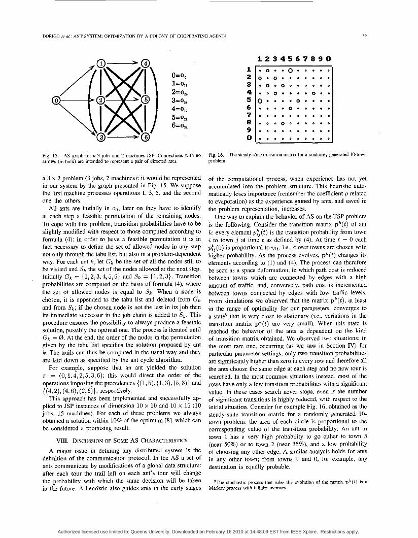
To apply the AS to JSP we chose the following representation. A JSP with M machines, J jobs and operation set 0 is represented as a directed weighted graph Q = (0’ ,A) where 0’ = 0 U {oo}, and A is the set of arcs that connect 00 with the first operation of each job and that completely connect the nodes of 0 except for the nodes belonging to a same job. Nodes belonging to a same job are connected in sequence (that is, a node is only connected to its immediate successor, see Fig. 15). Note that graph Q is not the graph with cliques representing machines that is usually utilized to represent the JSP. Node 00 is necessary in order to specify which job will be scheduled first, in case several jobs have their first operation on the same machine. We have therefore N + 1 nodes and 7 + IJI arcs, where all the nodes are painvise connected except 00, which is connected only to the first operation of each job. Each arc is weighted by a pair of numbers, {?-kL,Vkl}. The first, T ~ L , is the trail level, while the second is the visibility v k l , and is computed according to a desirability measure derived from a greedy problem specific heuristic like the Longest Processing Time or the Shortest Completion Time. The order in which the nodes are visited by each ant specifies the proposed solution. For instance, consider

Job-Shop Scheduling Problem:

N(N-1)


DORIGO et al.: ANT SYSTEM OPTIMIZATION BY A COLONY OF COOPERATING AGENTS

-

39

o=o, l=oll 2= 0,

3= 0 ,

4= O,,

5= 0,

6= o , ~

1 2 3 4 5 6 7 8 9 0

1 2 3 4 5 6 7 8 9 0 ~ 0 0 0 0 0 0 0 0 0 0

0 0 0 0 0 0 0 0 0 0

O O o O o o o o o o

0 0 0 0 0 0 0 0 0 0

~ 0 0 0 0 0 0 0 0 0

0 0 0 0 0 0 0 0 0 0

0 0 0 0 0 0 0 0 0 0

0 0 0 0 0 0 0 0 0 0

0 0 0 0 0 0 0 0 0 0

0 0 0 0 0 0 0 0 0 0

Fig. 15. arrows (in bold) are intended to represent a pair of directed arcs.

AS graph for a 3 jobs and 2 machines JSP. Connections with no Fig. 16. problem.

The steady-state transition matrix for a randomly generated lo-town

a 3 x 2 problem (3 jobs, 2 machines): it would be represented in our system by the graph presented in Fig. 15. We suppose the first machine processes operations 1, 3, 5, and the second one the others.

All ants are initially in 00; later on they have to identify at each step a feasible permutation of the remaining nodes. To cope with this problem, transition probabilities have to be slightly modified with respect to those computed according to formula (4): in order to have a feasible permutation it is in fact necessary to define the set of allowed nodes in any step not only through the tabu list, but also in a problem-dependent way. For each ant k , let Gk be the set of all the nodes still to be visited and SI, the set of the nodes allowed at the next step. Initially Gk = {1,2,3,4,5,6} and sk = {1,2,3}. Transition probabilities are computed on the basis of formula (4), where the set of allowed nodes is equal to s k . When a node is chosen, it is appended to the tabu list and deleted from Gk and from S k ; if the chosen node is not the last in its job then its immediate successor in the job chain is added to S k . This procedure ensures the possibility to always produce a feasible solution, possibly the optimal one. The process is iterated until Gk = @. At the end, the order of the nodes in the permutation given by the tabu list specifies the solution proposed by ant k . The trails can thus be computed in the usual way and they are laid down as specified by the ant cycle algorithm.

For example, suppose that an ant yielded the solution 7r = (0,1,4,2,5,3,6); this would direct the order of the operations imposing the precedences { ( 1,5), ( 1,3), (5,3)} and {(4,2), (4,6), (2,6)}, respectively.

This approach has been implemented and successfully applied to JSP instances of dimension 10 x 10 and 10 x 15 (10 jobs, 15 machines). For each of these problems we always obtained a solution within 10% of the optimum [8], which can be considered a promising result.

VIII. DISCUSSION OF SOME AS CHARACTERISTICS

A major issue in defining any distributed system is the definition of the communication protocol. In the AS a set of ants communicate by modifications of a global data structure: after each tour the trail left on each ant’s tour will change the probability with which the same decision will be taken in the future. A heuristic also guides ants in the early stages

of the computational process, when experience has not yet accumulated into the problem structure. This heuristic auto- matically loses importance (remember the coefficient p related to evaporation) as the experience gained by ants, and saved in the problem representation, increases.

One way to explain the behavior of AS on the TSP problem is the following. Consider the transition matrix pk(t) of ant k : every element p f j ( t ) is the transition probability from town i to town j at time t as defined by (4). At time t = 0 each pt3 (0) is proportional to v z j , i.e., closer towns are chosen with higher probability. As the process evolves, p k ( t ) changes its elements according to (1) and (4). The process can therefore be seen as a space deformation, in which path cost is reduced between towns which are connected by edges with a high amount of traffic, and, conversely, path cost is incremented between towns connected by edges with low traffic levels. From simulations we observed that the matrix p k ( t ) , at least in the range of optimality for our parameters, converges to a state’ that is very close to stationary (i.e., variations in the transition matrix p k ( t ) are very small). When this state is reached the behavior of the ants is dependent on the kind of transition matrix obtained. We observed two situations: in the most rare one, occurring (as we saw in Section IV) for particular parameter settings, only two transition probabilities are significantly higher than zero in every row and therefore all the ants choose the same edge at each step and no new tour is searched. In the most common situations instead, most of the rows have only a few transition probabilities with a significant value. In these cases search never stops, even if the number of significant transitions is highly reduced, with respect to the initial situation. Consider for example Fig. 16, obtained as the steady-state transition matrix for a randomly generated 10- town problem: the area of each circle is proportional to the corresponding value of the transition probability. An ant in town 1 has a very high probability to go either to town 5 (near 50%) or to town 2 (near 35%), and a low probability of choosing any other edge. A similar analysis holds for ants in any other town; from towns 9 and 0, for example, any destination is equally probable.

9The stochastic process that rules the evolution of the matrix p k ( t ) is a Markov process with infinitc memory.


40 IEEE TRANSACTIONS ON SYSTEMS, MAN, AND CYBERNETICS-PART B CYBERNETICS, VOL 26, NO 1, FEBRUARY 1996

Another way to interpret how the algorithm works is to imagine having some kind of probabilistic superimposition of effects: each ant, if isolated (that is, if Q = 0), would move with a local, greedy rule. This greedy rule guarantees only locally optimal moves and will practically always lead to bad final results. The reason the rule doesn’t work is that greedy local improvements lead to very bad final steps (an ant is constrained to make a closed tour and therefore choices for the final steps are constrained by early steps). So the tour followed by an ant ruled by a greedy policy is composed of some (initial) parts that are very good and some (final) parts that are not. If we now consider the effect of the simultaneous presence of many ants, then each one contributes to the trail distribution. Good parts of paths will be followed by many ants and therefore they receive a great amount of trail. On the contrary, bad parts of paths are chosen by ants only when they are obliged by constraint satisfaction (remember the tabu list); these edges will therefore receive trail from only a few ants.

IX. CONCLUSION This paper introduces a new search methodology based on

a distributed autocatalytic process and its application to the solution of a classical optimization problem. The general idea underlying the Ant System paradigm is that of a population of agents each guided by an autocatalytic process directed by a greedy force. Were an agent alone, the autocatalytic process and the greedy force would tend to make the agent converge to a suboptimal tour with exponential speed. When agents interact it appears that the greedy force can give the right suggestions to the autocatalytic process and facilitate quick convergence to very good, often optimal, solutions without getting stuck in local optima. We have speculated that this behavior could be due to the fact that information gained by agents during the search1 process is used to modify the problem representation and in this way to reduce the region of the space considered by the search process. Even if no tour is completely excluded, bad tours become highly improbable, and the agents search only in the neighborhood of good solutions.

The main contributions of this paper are the following. i)

ii)

We employ positive feedback as a search and optimization tool. The idea is that if at a given point an agent (ant) has to choose between different options and the one actually chosen results to be good, then in the future that choice will appear more desirable than it was before”. We show how synergy can arise and be useful in distributed systems. In the AS the effectiveness of the search carried out by a given number of cooperative ants is greater than that of the search carried out by the same number of ants, each one acting independently from the others.

iii) We show how to apply the AS to different combinatorial optimization problems. After introducing the AS by an

“Reinforcement of this nature is used by the reproduction-selection mechanism in evolutionary algorithms [23], [30], [33]. The main difference is that in evolutionary algorithms it is applied to favor (or disfavor) complete solutions, while in AS it is used to build solutions.

application to the TSP, we show how to apply it to the ATSP, the QAP, and the JSP.

We believe our approach to be a very promising one because of its generality (it can be applied to many different problenis, see Section VH), and because of its effectiveness in finding very good solutions to difficult problems.

Related work can be classified in the following major areas: * studies of social animal behavior; * research in “natural heuristic algorithms”;

stochastic optimization. As already pointed out the research on behavior of social

animals is to be considered as a source of inspiration and as a useful metaphor to explain our ideas. We believe that, especially if we are interested in designing inherently parallel algorithms, observation of natural systems can be an invaluable source of inspiration. Neural networks [32], genetic algorithms [23], evolution strategies [30, 331, immune networks [3], simulated annealing [24] are only some examples of models with a “natural flavor”. The main characteristics, which are at least partially shared by members of this class of algorithms, are the use of a natural metaphor, inherent parallelism, stochastic nature, adaptivity, and the use of positive feedback. Our algorithm can be considered as a new member of this class. All this work in “natural optimization” [ 12, 91 fits within the more general research area of stochastic optimization, in which the quest for optimality is traded for computational efficiency.

ACKNOWLEDGMENT The authors would like to thank two of the reviewers for

the many useful comments on the first version of this paper. We also thank Thomas Back, Hughes Bersini, Jean-Louis Deneubourg, Frank Hoffmeister, Mauro Leoncini, Francesco Maffioli, Bernard Manderik, Giovanni Manzini, Daniele Mon- tanari, Hans-Paul Schwefel and Frank Smieja for the discus- sions and the many useful comments on early versions of this paper.

REFERENCES

E. H. L. Aarts and J. H. M. Korst, Simulated Annealing and Boltzmann Machines. New York Wiley, 1988. J. L. Bentley, “Fast algorithms for geometric traveling salesman problems,” ORSA J. Computing, vol. 4, no. 4, pp. 387411, 1992. H. Bersini and F. J. Varela, “The immune recruitment mechanism: A selective evolutionary strategy,” in Proc. Fourth Int. Conf Genetic Algorithms. San Mateo, CA: Morgan Kaufmann, 1991, pp. 520-526. S. C. Boyd, W. R. Pulleyblank and G. Cornuejols, Travel Software Package, Carleton University, 1989. R. E. Burkhard, “Quadratic assignment problems,” Europ. J. Oper. Res., vol. 15, pp. 283-289, 1984. A. Colomi, M. Dorigo and V. Maniezzo, “Distributed optimization by ant colonies,” in Proc. First Europ. Conf ArtiJicial Life, F. Varela and P. Bourgine, Eds. A. Colomi, M. Dorigo and V. Maniezzo, “An investigation of some properties of an ant algorithm,” in Proc. Parallel Problem Solving from Nature Conference (PPSN ’92), R. Manner and B. Manderick Eds. Brussels, Belgium: Elsevier, 1992, pp. 509-520. A. Colorni, M. Dorigo, V. Maniezzo and M. Trubian, “Ant system for job-Shop scheduling,” JORBEL-Belgian J. Oper. Res., Statist. Conzp. Sci., vol. 34, no. 1, pp. 39-53. A. Colorni, M. Dorigo, F. Maffioli, V. Maniezzo, G. Righini and M. Trubian, “Heuristics from nature for hard combinatorial problems,” Tech. Rep. 93425, Dip. Elettronica e Informazione, Politecnico di Milano, Italy, 1993.

Paris, France: Elsevier, 1991, pp. 134-142.


DORIGO et al.: ANT SYSTEM OPTIMIZATION BY A COLONY OF COOPERATI?

[lo] J. L. Denebourg, J. M. Pasteels and J. C. Verhaeghe, “Probabilistic behavior in ants: A strategy of errors?,” J. Theoret. Biol., vol. 105, pp. 259-271, 1983.

[ l l ] J. L. Denebourg and S. Goss, “Collective patterns and decision-making,” Ethology, Ecology & Evolution, vol. 1, pp. 295-311, 1989.

[12] M. Dorigo, “Optimization, learning and natural algorithms,” Ph.D. Thesis, Dip. Elettronica e Informazione, Politecnico di Milano, Italy, 1992.

[13] M. Dorigo, V. Maniezzo and A. Colorni, “Positive feedback as a search strategy,” Tech. Rep. 91-016, Politecnico di Milano, 1991.

[14] S. Eilon, T. H. Watson-Gandy and N. Christofides, “Distribution man- agement: Mathematical modeling and practical analysis,” Oper. Res. Quart., vol. 20, pp. 37-53, 1969.

[15] A. E. Elshafei, “Hospital layout as a quadratic assignment problem,” Oper. Res. Quart., vol. 28, pp. 167-179, 1977.

[16] M. Fischetti and P. Toth, “An additive bounding procedure for the asymmetric travelling salesman problem,” Mathemat. Prog., vol. 53,

[17] F. Glover, “Tabu Search-Part I,” ORSA J. Computing, vol. 1, no. 3,

[18] -, “Tabu Search-Part 11,” ORSA J. Computing, vol. 2, no. 1, pp.

[ 191 D. E. Goldberg, Genetic Algorithms in Search, Optimization & Machine Learning. Reading, MA: Addison-Wesley, 1989.

[20] B. Golden and W. Stewart, “Empiric analysis of heuristics,” in The Travelling Salesman Problem, E. L. Lawler, J. K. Lenstra, A. H. G. Rinnooy-Kan, D. B. Shmoys Eds.. New York Wiley, 1985.

1211 S. Goss, R. Beckers, J. L. Denebourg, S. Aron and J. M. Pasteels, “How trail laying and trail following can solve foraging problems for ant colonies,” in Behavioral Mechanisms of Food Selection, R. N. Hughes Ed., NATO-AS1 Series. Berlin: Springer-Verlag, vol. G 20, 1990.

[22] R. L. Graham, E. L. Lawler, J. K. Lenstra and A. H. G. Rinnooy Kan, “Optimization and approximation in deterministic sequencing and scheduling: A survey,’’ in Annals Disc. Math., vol. 5, pp. 287-326, 1979.

[23] J. H. Holland, Adaptation in Natural and Art$cial Systems. Ann Arbor, MI: The University of Michigan Press, 1975.

[24] S. Kirkpatrick, C. D. Gelatt and M. P. Vecchi, “Optimization by simulated annealing,” Sci., vol. 220, pp. 671-680, 1983.

[25] J. Krarup, P. M. Pruzan, “Computer-aided layout design,” Mathemat. Prog. Study, vol. 9, pp. 85-94, 1978.

[26] E. L. Lawler, J. K. Lenstra, A. H. G. Rinnooy-Kan and D. B. Shmoys Eds., The Travelling Salesman Problem. New York: Wiley, 1985.

[27] S. Lin and B. W. Kernighan, “An effective heuristic algorithm for the TSP,” Oper. Res., vol. 21, 498-516, 1973.

[28] V. Maniezzo, A. Colorni and M. Dorigo, “The ant system applied to the quadratic assignment problem,” Tech. Rep. IRIDIN94-28, Universitk Libre de Bruxelles, Belgium, 1994.

[29] C. E. Nugent, T. E. Vollmann and J. Ruml, “An experimental comparison of techniques for the assignment of facilities to locations,” Oper. Res.,

[30] I. Rechenberg, Evolutionsstrategie. Stuttgart: Fromman-Holzbog, 1973.

[3 11 G. Reinelt, TSPLIB 1.0, Institut fur Mathematik, Universitat Augsburg, Germany, 1990.

[32] D. E. Rumelhart and J. L. McLelland, Parallel Distributed Processing: Explorations in the Microstructure of Cogniton. Cambridge, MA: MIT Press, 1986.

[33] H.-P. Schwefel, “Evolutionsstrategie und numerische optimierung,” Ph.D. Thesis, Technische Universitat Berlin, 1975. Also available as Numerical Optimization of Computer Models. New York Wiley, 198 1.

[34] D. Whitley, T. Starkweather and D. Fuquay, “Scheduling problems and travelling salesman: The genetic edge recombination operator,” in Proc. Third Int. Con$ on Genetic Algorithms. San Mateo, C A Morgan Kaufmann, 1989.

pp. 173-197, 1992.

pp. 190-206, 1989.

4-32, 1990.

vol. 16, pp. 150-173, 1968.

\IG AGENTS 41

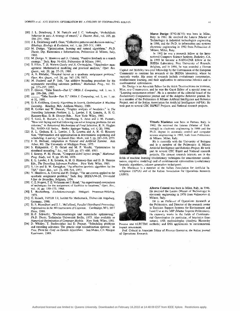
Marco Dorigo (S’92-M’93) was born in Milan, Italy, in 1961. He received the Laurea (Master of Technology) in industrial technologies engineering in 1986, and the Ph.D. in information and systems electronic engineering in 1992 from Politecnico di Milano, Milan, Italy.

In 1992 he was a research fellow at the Inter- national Computer Science Institute, Berkeley, CA. In 1993 he became a NATO-CNR fellow at the IRIDIA Laboratory, Free University of Brussels, Belgium, and in 1994, he was awarded a Human

Capital and Mobility two-year fellowship by the Commission of the European Community to continue his research at the IRIDIA laboratory, where he currently works. His areas of research include evolutionary computation, reinforcement learning, and their application to autonomous robotics and to combinatorial optimization.

Dr. Dorigo is an Associate Editor for the IEEE TRANSACTIONS ON SYSTEMS, MAN, AND CYBERNETICS, and he was the Guest Editor of a special issue on “Learning autonomous robots”. He is a member of the editorial board of the Evolutionary Computation journal and of the Adaptive Behavior journal. He is a member of the Politecnico di Milano Artificial Intelligence and Robotics Project, and of the Italian Association for Artificial Intelligence (AI*IA). He took part to several CEC ESPRIT Projects, and National research projects.

Vittorio Maniezzo was born in Ferrara, Italy, in 1962. He received the Laurea (Master of Tech- nology) in electronic engineering in 1986 and the Ph.D. degree in automatic control and computer science engineering in 1993, both from Politecnico di Milano, Milan, Italy.

He is currently with the University of Bologna and is a member of the Politecnico di Milano Artificial Intelligence and Robotics Project. He took part to several CEC Esprit and National research projects. His current research interests are in the

fields of machine learning (evolutionary techniques for sensonmotor coordi- nation, cognitive modeling) and of combinatorial optimization (evolutionary heuristic algorithms, column generation techniques).

Dr. Maniezzo is a member of the Italian Association for Artificial In- telligence (AI*IA) and of the Italian Association for Operations Research (AIRO).

Albert0 Colorni was born in Milan, Italy, in 1946. He received the Laurea (Master of Technology) in electronic engineering in 1970 from Politecnico di Milano, Italy.

He is an Professor of Operations Research at the Politecnico, and Director of the research center in Decision Support Systems for Environment and Land Use at the ME’ (Master Imprese-Politecnico). He currently works in the fields of Combinato- rial Optimization (in particular, of heuristics from nature), DSS methodologies (Analytic Hierarchy

Process and ELECTRE methods) and DSS applications to environmental impact assessment.

Prof. Colorni is Associate Editor OF Rccerca Operatcva, the Italian journal of Operations Research.


Documents

Ant System: Optimization by a Colony of Cooperating Agents