ANSYS - Välkommen till KTH · PDF fileBasic program structure ... Start Mechanical APDL (ANSYS). Your model can be saved in a database by specifying your working directory (the

INTRODUCTION TO A FINITE ELEMENT

ANALYSIS PROGRAM:

ANSYS

KTH, Department of Solid Mechanics

2(19)

Table of contents

Introduction .................................................................................................................... 3

Short history ................................................................................................................... 3

Basic program structure ................................................................................................. 3

Preprocessor ............................................................................................................... 5

Solution processor ...................................................................................................... 5

Postprocessor ............................................................................................................. 6

Tutorial 1: Truss problem .............................................................................................. 7

Geometry .................................................................................................................... 8

Material .................................................................................................................... 10

Element type ............................................................................................................ 11

Mesh ......................................................................................................................... 12

Loads ........................................................................................................................ 13

Solution .................................................................................................................... 13

Results ...................................................................................................................... 13

Tutorial 2: Beam problem ............................................................................................ 16

Geometry .................................................................................................................. 16

Material .................................................................................................................... 16

Element type ............................................................................................................ 17

Mesh ......................................................................................................................... 17

Loads ........................................................................................................................ 17

Solution .................................................................................................................... 18

Results ...................................................................................................................... 18


3(19)

Introduction

The following pages should give you a brief and basic introduction to the architecture

and structure of a commercial finite element analysis program. The basic ideas can be

applied in most programs but examples are taken from the software ANSYS (version

12). Here we will only focus on structural mechanics in ANSYS. Note also that many

steps can be done in several other ways than what is presented here.

Short history

The usage of the Finite Element Method as a tool to solve engineering problems

commercially in industrial applications is quite new. It was used in the late 1950’s and

early 60’s, but not in the same way as it is today. The calculations were, at that time,

carried out by hand and the method was force based, not displacement based as we

use it today. In the mid 60’s, very specialized computer programs were used to

perform the analysis. The 1970’s was the time when commercial programs started to

emerge. At first, FEM was limited to expensive mainframe computers owned by the

aeronautics, automotive, defense and nuclear industries. However, in the late 70’s

more companies started to use the FEM, and since then, the usage has grown very

rapidly.

Today commercial programs are large and very powerful, complex problems

can be solved by one person on a PC. Many of them have the ability to handle

different kinds of physical phenomena such as thermo mechanics, electro mechanics

and structural mechanics. One often talks about multiphysics, where different kinds of

physical phenomena are coupled in the same analysis. There are many available

commercial programs, ABAQUS, FLUENT, Comsol Multiphysics, and ANSYS are

just a few examples. A full license of a finite element analysis program usually cost

on the order of several tens of thousands of Euros. ANSYS is a widely used

commercial general-purpose finite element analysis program.

Basic program structure

Treatment of engineering problems generally contains three main parts: create a

model, solve the problem, analyze the results. ANSYS, like many other FE-programs,

is also divided into three main parts (processors) which are called preprocessor,

solution processor, postprocessor. Other software may contain only the preprocessing

part or only the postprocessing part. During the analysis you will communicate with

ANSYS via a Graphical User Interface (GUI), which is described below and seen in

Figure 1.


4(19)

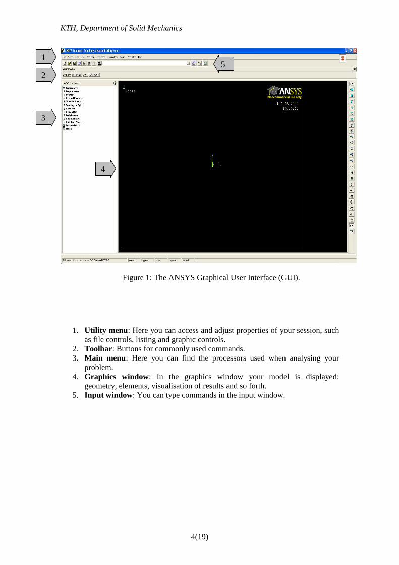
Figure 1: The ANSYS Graphical User Interface (GUI).

1. Utility menu: Here you can access and adjust properties of your session, such

as file controls, listing and graphic controls.

2. Toolbar: Buttons for commonly used commands.

3. Main menu: Here you can find the processors used when analysing your

problem.

4. Graphics window: In the graphics window your model is displayed:

geometry, elements, visualisation of results and so forth.

5. Input window: You can type commands in the input window.

1

2

3

4

5


5(19)

Preprocessor

Within the preprocessor the model is set up. It usually includes a number of steps in

the following order:

Build geometry. Depending on whether the problem geometry is one, two or

three dimensional, the geometry consists of creating lines, areas or volumes.

These geometries can then, if necessary, be used to create other geometries by

the use of boolean operations. The key idea when building the geometry like

this is to simplify the generation of the element mesh. Hence, this step is

optional but most often used. Nodes and elements can however be created

from coordinates only.

Define materials. A material is defined by its material constants. Every

element has to be assigned a particular material.

Generate element mesh. The problem is discretized with nodal points. The

nodes are connected to form finite elements, which together form the material

volume. Depending on the problem and the assumptions that are made, the

element type has to be determined. Common element types are truss, beam,

plate, shell and solid elements. Each element type may contain several

subtypes, e.g. 2D 4-noded solid, 3D 20-noded solid elements. Therefore, care

has to be taken when the element type is chosen.

The element mesh can in ANSYS be created in several ways. The most

common way is that it is automatically created, however more or less

controlled. For example you can specify a certain number of elements in a

specific area, or you can force the mesh generator to maintain a specific

element size within an area. Certain element shapes or sizes are not

recommended and if these limits are violated, a warning will be generated in

ANSYS. It is up to the user to create a mesh which is able to generate results

with a sufficient degree of accuracy.

Solution processor

Here you solve the problem by gathering all specified information about the problem:

Apply loads: Boundary conditions are usually applied on nodes or elements.

The prescribed quantity can for example be force, traction, displacement,

moment, rotation. The loads may also be edited from the preprocessor in

ANSYS.

Obtain solution: The solution to the problem can be obtained if the whole

problem is defined.


6(19)

Postprocessor

Within this part of the analysis you can for example:

Visualize the results: For example, plot the deformed shape of the geometry

or stresses.

List the results: It is possible to list the results as tabular listings or file

printouts.


7(19)

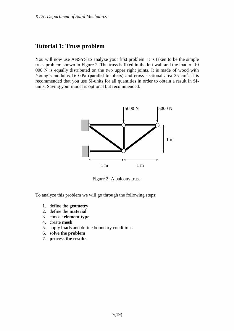
Tutorial 1: Truss problem

You will now use ANSYS to analyze your first problem. It is taken to be the simple

truss problem shown in Figure 2. The truss is fixed in the left wall and the load of 10

000 N is equally distributed on the two upper right joints. It is made of wood with

Young’s modulus 16 GPa (parallel to fibers) and cross sectional area 25 cm2. It is

recommended that you use SI-units for all quantities in order to obtain a result in SI-

units. Saving your model is optional but recommended.

Figure 2: A balcony truss.

To analyze this problem we will go through the following steps:

1. define the geometry

2. define the material

3. choose element type

4. create mesh

5. apply loads and define boundary conditions

6. solve the problem

7. process the results

5000 N 5000 N

1 m 1 m

1 m


8(19)

Start Mechanical APDL (ANSYS). Your model can be saved in a database by

specifying your working directory (the folder where you want your ANSYS files to be

saved) and a job name (every problem has a job name, for example, truss).

ANSYS Utility menu: File → Change directory …

ANSYS Utility menu: File → Change jobname …

Geometry

We will now draw the structure shown in Figure 2 by first defining keypoints and then

drawing lines between them. A visible working plane often makes the creation of the

geometry easier. Therefore:

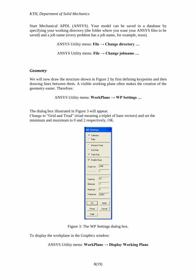
ANSYS Utility menu: WorkPlane → WP Settings …

The dialog box illustrated in Figure 3 will appear.

Change to “Grid and Triad” (triad meaning a triplet of base vectors) and set the

minimum and maximum to 0 and 2 respectively, OK.

Figure 3: The WP Settings dialog box.

To display the workplane in the Graphics window:

ANSYS Utility menu: WorkPlane → Display Working Plane


9(19)

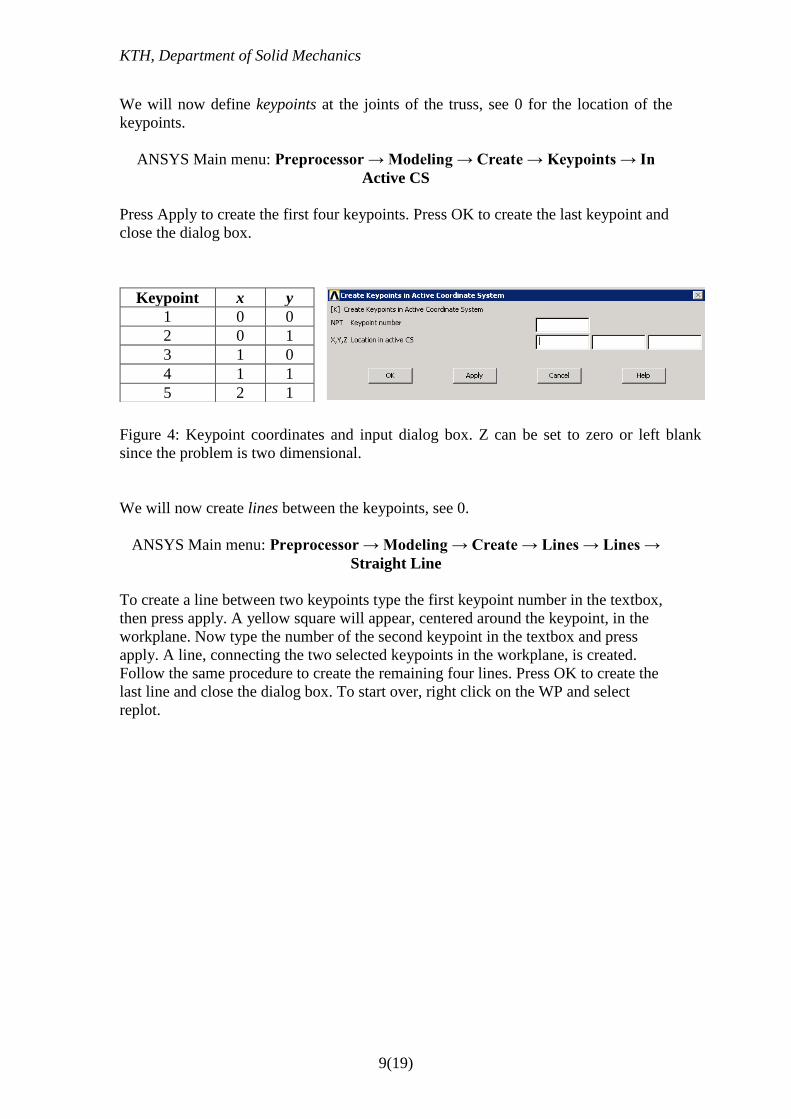
We will now define keypoints at the joints of the truss, see 0 for the location of the

keypoints.

ANSYS Main menu: Preprocessor → Modeling → Create → Keypoints → In

Active CS

Press Apply to create the first four keypoints. Press OK to create the last keypoint and

close the dialog box.

Figure 4: Keypoint coordinates and input dialog box. Z can be set to zero or left blank

since the problem is two dimensional.

Keypoint x y

1 0 0

2 0 1

3 1 0

4 1 1

5 2 1

We will now create lines between the keypoints, see 0.

ANSYS Main menu: Preprocessor → Modeling → Create → Lines → Lines →

Straight Line

To create a line between two keypoints type the first keypoint number in the textbox,

then press apply. A yellow square will appear, centered around the keypoint, in the

workplane. Now type the number of the second keypoint in the textbox and press

apply. A line, connecting the two selected keypoints in the workplane, is created.

Follow the same procedure to create the remaining four lines. Press OK to create the

last line and close the dialog box. To start over, right click on the WP and select

replot.


10(19)

Figure 5: Lines and keypoints.

Line KP1 KP2

1 1 3

2 2 4

3 4 5

4 4 3

5 2 3

6 3 5

Tip: You can check your geometry in the graphics display:

ANSYS Utility menu: Plot → Keypoints → Keypoints

or

ANSYS Utility menu: Plot → Lines

Numbering of lines and keypoints on the graphics display can be turned on and off in

the dialog box after selecting

ANSYS Utility menu: PlotCtrls → Numbering…

Material

We assume that the wood behaves linearly elastic. Define the: material model (that is

the properties of the material), and the material constants (Young’s modulus, and

Poisson’s ratio), see Figure 6:

ANSYS Main menu: Preprocessor → Material Props → Material Models


11(19)

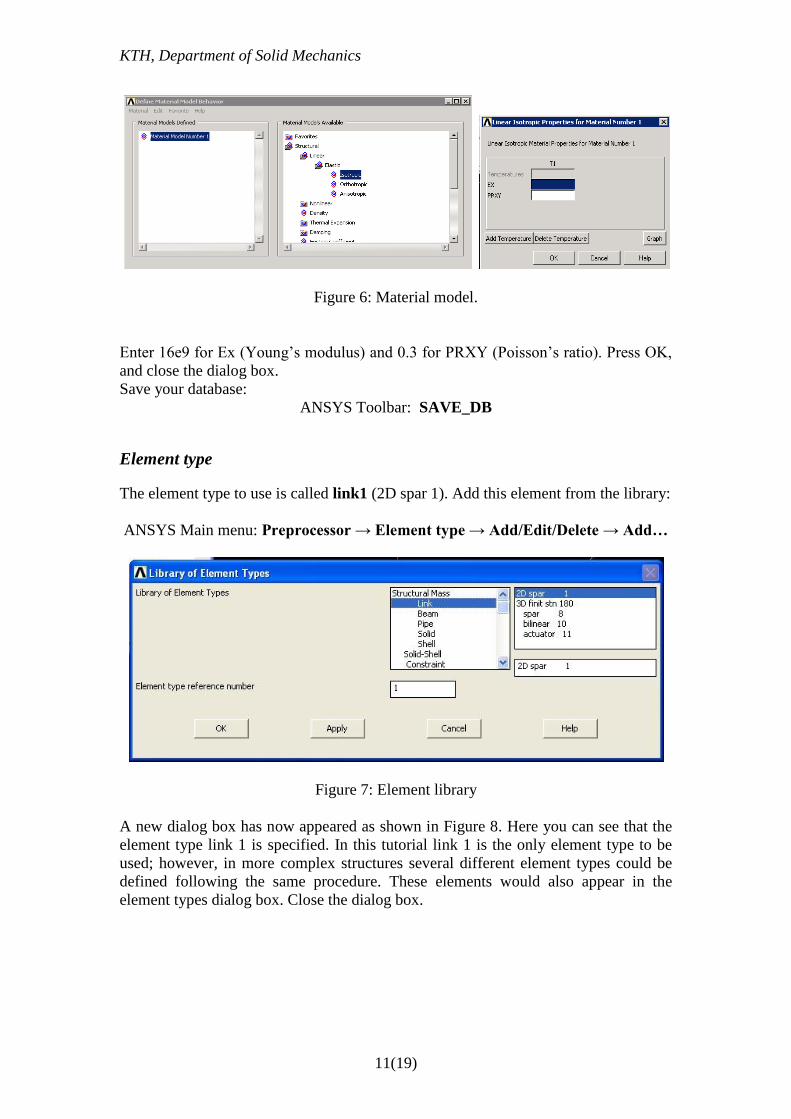
Figure 6: Material model.

Enter 16e9 for Ex (Young’s modulus) and 0.3 for PRXY (Poisson’s ratio). Press OK,

and close the dialog box.

Save your database:

ANSYS Toolbar: SAVE_DB

Element type

The element type to use is called link1 (2D spar 1). Add this element from the library:

ANSYS Main menu: Preprocessor → Element type → Add/Edit/Delete → Add…

Figure 7: Element library

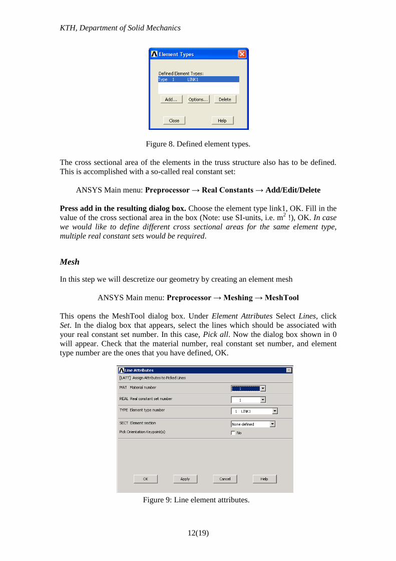
A new dialog box has now appeared as shown in Figure 8. Here you can see that the

element type link 1 is specified. In this tutorial link 1 is the only element type to be

used; however, in more complex structures several different element types could be

defined following the same procedure. These elements would also appear in the

element types dialog box. Close the dialog box.


12(19)

Figure 8. Defined element types.

The cross sectional area of the elements in the truss structure also has to be defined.

This is accomplished with a so-called real constant set:

ANSYS Main menu: Preprocessor → Real Constants → Add/Edit/Delete

Press add in the resulting dialog box. Choose the element type link1, OK. Fill in the

value of the cross sectional area in the box (Note: use SI-units, i.e. m2 !), OK. In case

we would like to define different cross sectional areas for the same element type,

multiple real constant sets would be required.

Mesh

In this step we will descretize our geometry by creating an element mesh

ANSYS Main menu: Preprocessor → Meshing → MeshTool

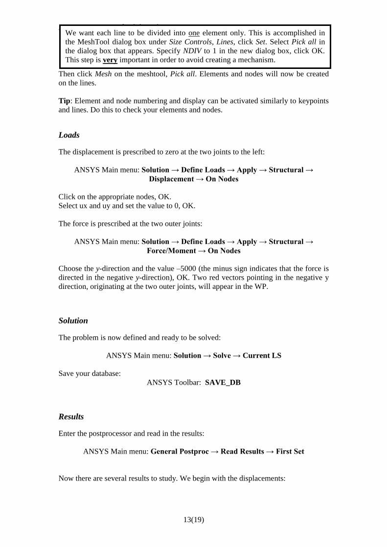
This opens the MeshTool dialog box. Under Element Attributes Select Lines, click

Set. In the dialog box that appears, select the lines which should be associated with

your real constant set number. In this case, Pick all. Now the dialog box shown in 0

will appear. Check that the material number, real constant set number, and element

type number are the ones that you have defined, OK.

Figure 9: Line element attributes.


13(19)

Then click Mesh on the meshtool, Pick all. Elements and nodes will now be created

on the lines.

Tip: Element and node numbering and display can be activated similarly to keypoints

and lines. Do this to check your elements and nodes.

Loads

The displacement is prescribed to zero at the two joints to the left:

ANSYS Main menu: Solution → Define Loads → Apply → Structural →

Displacement → On Nodes

Click on the appropriate nodes, OK.

Select ux and uy and set the value to 0, OK.

The force is prescribed at the two outer joints:


Force/Moment → On Nodes

Choose the y-direction and the value –5000 (the minus sign indicates that the force is

directed in the negative y-direction), OK. Two red vectors pointing in the negative y

direction, originating at the two outer joints, will appear in the WP.

Solution

The problem is now defined and ready to be solved:

ANSYS Main menu: Solution → Solve → Current LS

Save your database:

ANSYS Toolbar: SAVE_DB

Results

Enter the postprocessor and read in the results:

ANSYS Main menu: General Postproc → Read Results → First Set

Now there are several results to study. We begin with the displacements:

We want each line to be divided into one element only. This is accomplished in

the MeshTool dialog box under Size Controls, Lines, click Set. Select Pick all in

the dialog box that appears. Specify NDIV to 1 in the new dialog box, click OK.

This step is very important in order to avoid creating a mechanism.


14(19)

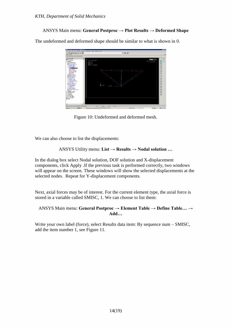
ANSYS Main menu: General Postproc → Plot Results → Deformed Shape

The undeformed and deformed shape should be similar to what is shown in 0.

Figure 10: Undeformed and deformed mesh.

We can also choose to list the displacements:

ANSYS Utility menu: List → Results → Nodal solution …

In the dialog box select Nodal solution, DOF solution and X-displacement

components, click Apply .If the previous task is performed correctly, two windows

will appear on the screen. These windows will show the selected displacements at the

selected nodes. Repeat for Y-displacement components.

Next, axial forces may be of interest. For the current element type, the axial force is

stored in a variable called SMISC, 1. We can choose to list them:

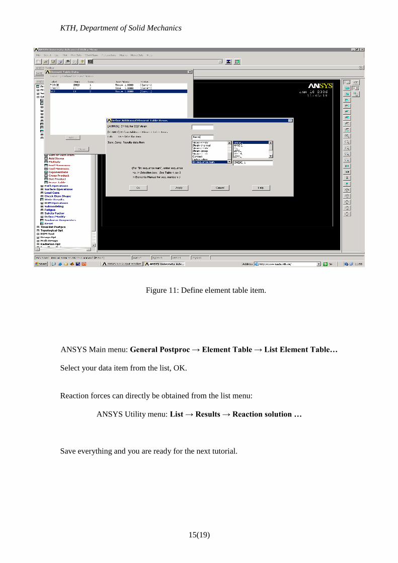
ANSYS Main menu: General Postproc → Element Table → Define Table… →

Add…

Write your own label (force), select Results data item: By sequence num – SMISC,

add the item number 1, see Figure 11.


15(19)

Figure 11: Define element table item.

ANSYS Main menu: General Postproc → Element Table → List Element Table…

Select your data item from the list, OK.

Reaction forces can directly be obtained from the list menu:

ANSYS Utility menu: List → Results → Reaction solution …

Save everything and you are ready for the next tutorial.


16(19)

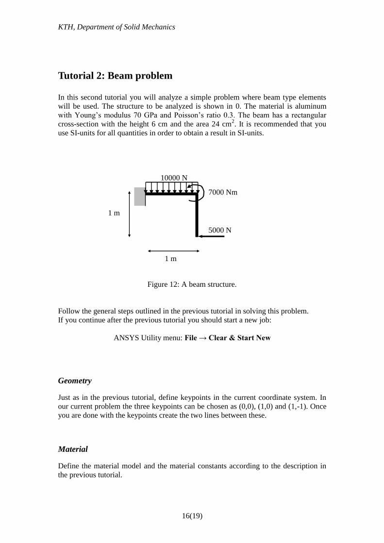
Tutorial 2: Beam problem

In this second tutorial you will analyze a simple problem where beam type elements

will be used. The structure to be analyzed is shown in 0. The material is aluminum

with Young’s modulus 70 GPa and Poisson’s ratio 0.3. The beam has a rectangular

cross-section with the height 6 cm and the area 24 cm2. It is recommended that you

use SI-units for all quantities in order to obtain a result in SI-units.

Figure 12: A beam structure.

Follow the general steps outlined in the previous tutorial in solving this problem.

If you continue after the previous tutorial you should start a new job:

ANSYS Utility menu: File → Clear & Start New

Geometry

Just as in the previous tutorial, define keypoints in the current coordinate system. In

our current problem the three keypoints can be chosen as (0,0), (1,0) and (1,-1). Once

you are done with the keypoints create the two lines between these.

Material

Define the material model and the material constants according to the description in

the previous tutorial.

1 m

1 m

5000 N

10000 N

7000 Nm


17(19)

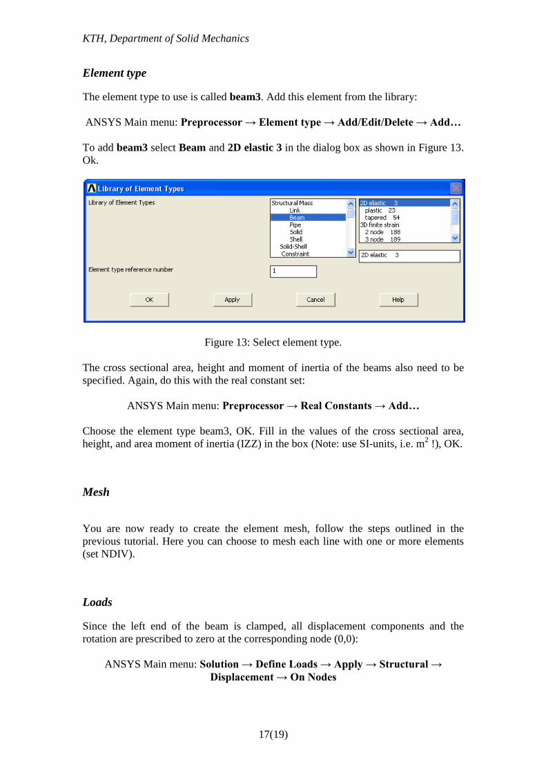
Element type

The element type to use is called beam3. Add this element from the library:

ANSYS Main menu: Preprocessor → Element type → Add/Edit/Delete → Add…

To add beam3 select Beam and 2D elastic 3 in the dialog box as shown in Figure 13.

Ok.

Figure 13: Select element type.

The cross sectional area, height and moment of inertia of the beams also need to be

specified. Again, do this with the real constant set:

ANSYS Main menu: Preprocessor → Real Constants → Add…

Choose the element type beam3, OK. Fill in the values of the cross sectional area,

height, and area moment of inertia (IZZ) in the box (Note: use SI-units, i.e. m2 !), OK.

Mesh

You are now ready to create the element mesh, follow the steps outlined in the

previous tutorial. Here you can choose to mesh each line with one or more elements

(set NDIV).

Loads

Since the left end of the beam is clamped, all displacement components and the

rotation are prescribed to zero at the corresponding node (0,0):


Displacement → On Nodes


18(19)

Click on the appropriate node, OK. Select All DOF and set the value to 0, OK.

Apply the force 5000 in the x direction on the node at (1,-1), follow the steps in the

previous tutorial.

Now we will apply the moment at the coordinate (1,0):


Force/Moment → On Nodes

Click on the appropriate node, OK. Choose Mz and the value 7000, OK. A small cross

will appear on the node to indicate the applied moment.

Finally we will apply the pressure on the top beam. Choose

ANSYS Main menu: Solution → Define Loads → Apply → Structural → Pressure

→ On Beams

Select the appropriate line, OK. In the dialog box that appears enter 10000 for VALI

and click OK. Note that you can specify a linearly distributed load by entering a value

for VALJ, which is the value at the other (right) end of the line. As our load is uniform

that field should be left blank. When finished, the uniform load will show up on the

horizontal element.

Solution

The problem is now defined and ready to be solved:

ANSYS Main menu: Solution → Solve → Current LS

Results

Enter the postprocessor and read in the results:

ANSYS Main menu: General Postproc → Read Results → First Set

Now there are several results to study. Plot the deformed and undeformed shapes, this

has been described earlier.

Next, axial forces may be of interest. We can choose to list them:

ANSYS Main menu: General Postproc → Element Table → Define Table… →

Add…

Write your own label (force), select Results data item: By sequence num – SMISC, 1.

Add results for the moment by repeating the above steps and add the data items

SMISC, 6 and SMISC, 12. For the current element type these variables define the

bending moment at the left and right end of the element, respectively.


19(19)

These items can be studied by listing them

ANSYS Main menu: General Postproc → Element Table → List Element Table…

Select your data item from the list, OK.

It is also possible to plot the moment distribution for the beams:

ANSYS Main menu: General Postproc → Plot Results→ Contour Plot → Line

Elem Res

Select SMIS6 for “LabI” and SMIS12 for “LabJ”, OK.

Nodal solutions can be listed as outlined previously. In addition to x- and y-

displacements we may also list the z-component of rotation:

ANSYS Utility menu: List → Results → Reaction solution …

Documents

ANSYS - Välkommen till KTH · PDF fileBasic program structure ... Start Mechanical APDL (ANSYS). Your model can be saved in a database by specifying your working directory (the