Answer Set Programming: A Primer?

Thomas Eiter1, Giovambattista Ianni2, and Thomas Krennwallner1

1 Institut fur Informationssysteme, Technische Universitat WienFavoritenstraße 9-11, A-1040 Vienna, Austria{eiter,tkren}@kr.tuwien.ac.at

2 Dipartimento di Matematica, Universita della Calabria, I-87036 Rende (CS), Italyianni@mat.unical.it

Abstract. Answer Set Programming (ASP) is a declarative problem solving para-digm, rooted in Logic Programming and Nonmonotonic Reasoning, which hasbeen gaining increasing attention during the last years. This article is a gentleintroduction to the subject; it starts with motivation and follows the historicaldevelopment of the challenge of defining a semantics for logic programs withnegation. It looks into positive programs over stratified programs to arbitraryprograms, and then proceeds to extensions with two kinds of negation (namedweak and strong negation), and disjunction in rule heads. The second part thenconsiders the ASP paradigm itself, and describes the basic idea. It shows someprogramming techniques and briefly overviews Answer Set solvers. The third partis devoted to ASP in the context of the Semantic Web, presenting some formalismsand mentioning some applications in this area. The article concludes with issuesof current and future ASP research.

1 Introduction

Over the the last years, Answer Set Programming (ASP) [1–5] has emerged as a declar-ative problem solving paradigm that has its roots in Logic Programming and Non-monotonic Reasoning. This particular way of programming, in a language which issometimes called AnsProlog (or simply A-Prolog) [6, 7], is well-suited for modelingand (automatically) solving problems which involve common sense reasoning: it hasbeen fruitfully applied to a range of applications (for more details, see Section 6). Anumber of extensions of the ASP core language, which goes back to the seminal paperby Gelfond and Lifschitz [8], have been developed (resulting in an AnsProlog∗ languagefamily). These extensions aim at increasing the expressiveness of the formalisms and/orproviding convenient constructs for application-specific problem representation; see,e.g., [9] for an account of such extensions.

The basic idea of ASP is to describe problem specifications by means of a non-monotonic logic program: solutions to instances of such a problem will be represented

? This is an updated version of the paper (with corrections) that appeared in the Proceedings ofthe 5th International Reasoning Web Summer School 2009, volume 5689 of LNCS, Springer.This work has been supported by the Austrian Science Fund (FWF) project P20840 & P20841,the EC ICT Integrated Project Ontorule (FP7 231875), and the Italian National Project InterlinkII04CG8AGG.

6 1 4 58 3 5 6

2 18 4 7 6

6 37 9 1 45 2

7 2 6 94 5 8 7

9 6 3 1 7 4 2 5 81 7 8 3 2 5 6 4 92 5 4 6 8 9 7 3 18 2 1 4 3 7 5 9 64 9 6 8 5 2 3 1 77 3 5 9 6 1 8 2 45 8 9 7 1 3 4 6 23 1 7 2 4 6 9 8 56 4 2 5 9 8 1 7 3

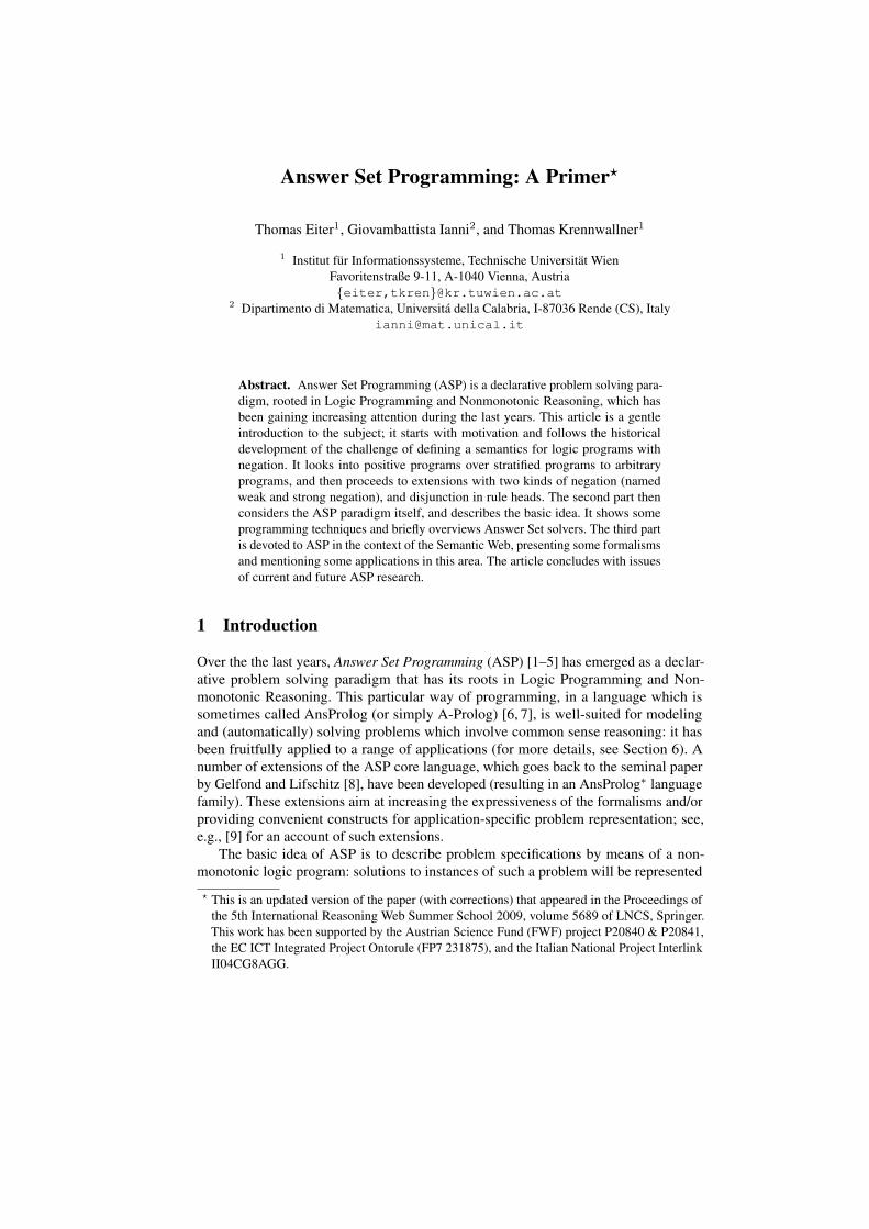
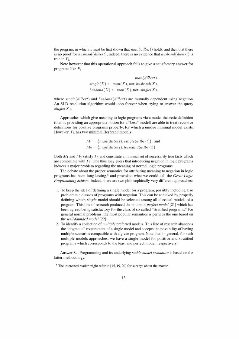
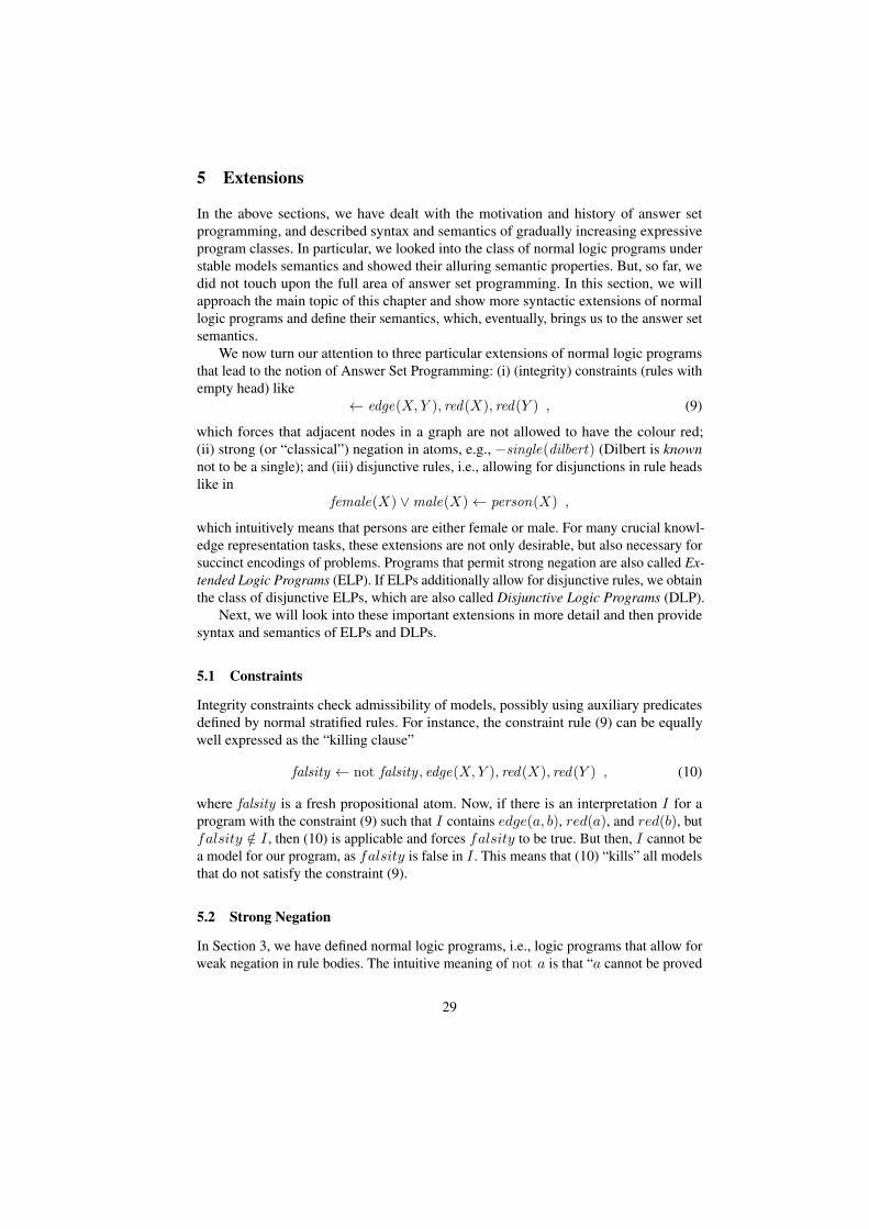
Fig. 1. Sudoku puzzle (left) and solution (right)

by the intended models of the program (the so-called answer sets, or stable models) athand. Rules and constraints, which describe the problem and its possible solutions ratherthan a concrete algorithm, are basic elements of such programs.

Such a problem encoding can be then fed into an answer set (AS) solver, whichcomputes some or multiple answer set(s) of the program, from which the solutions ofthe problem can easily be read off.

As a simple motivating example, consider the popular Sudoku game.3

Example 1 (Sudoku). In its original version, a Sudoku consists of a tableau that has 81cells arranged in a grid, which is divided into nine sub-tableaux (the blocks or regions)of equal size having nine fields each. The initial game setup has some of the entries filledwith numbers between 1 and 9 (see Figure 1, left, for an example).

The question is now whether the tableau can be completed in a way such that eachrow and each column shows every digits from 1 to 9 exactly once, and moreover thatalso each block has this property. An example for a completed Sudoku grid is on theright in Figure 1, which is the unique solution to the initial puzzle on the left.4

In general, the problem of solving Sudoku tables automatically appears to be non-trivial: in principle, one can devise a brute force algorithm that considers all possibleassignments and checks whether the solution constraint is satisfied. For a versatileprogrammer, it is not difficult to write a program in her favorite programming language,be it Java, C++, or some other language, to compute and print a solution to instances ofthis problem.

In this traditional, time-consuming approach, a human programmer receives aninformal specification of the problem at hand, such as the Sudoku above, and manuallyconverts it into imperative code that is able to solve instances of the problem. However,one might conceive to tackle this issue from a completely different perspective.

For instance, one can think of having access to appropriate means for directlydescribing the problem at hand in a declarative specification. This specification, ifproperly polished from ambiguities of natural language and expressed in a proper syntax,

3 This game has nowadays worldwide popularity, and world and national championships are heldin big tournaments each year across Europe.

4 To date, many variants of Sudoku emerged, like, e.g., color-Sudoku, Samurai-Sudoku, etc.

2

would be not much different in its meaning from the formulation of Sudoku of ourexample. Also, such a specification could be automatically executed, in the sense thatsome computational engine takes this specification as input, together with a probleminstance, and then produces a solution as output. In such a vision, the human programmerwould switch her focus from how to solve a problem to how to state a problem, which isa much easier and faster task. 5

The Prolog language, and its extensions conceived for handling constraints, can beseen at a first glance as tools for such “declarative problem solving.” Prolog is indeedwell-suited for this particular case.

There are however aspects which make the suitability of Prolog (with respect toAnsProlog) less apparent. Among such aspects, there is the fact that many commonproblems require preference handling (that is, the possibility to describe which solutionsare preferred to others with respect to some “quality” criterion), and to properly deal withincomplete information (that is, the ability to properly complete missing informationwith default assumptions, or with assumptions of falsity, or with using some notion ofundefinedness). The next example shows the impact of such aspects.

Example 2 (Social Dinner Example). Imagine the organizers of this course planninga fancy dinner for the course participants. To make the event a great success, theorganizers decide to ask the attendees to declare their personal wine preferences. Soon,the organizers become aware of the fact that there is no wine, which satisfies all of theparticipant preferences. Thus, they aim at automatically finding the cheapest selection ofbottles such that any attendee can have her preferred wine at the dinner. This solutionshould take into account that people usually like wine from their home country, but maynot like to drink it abroad.

The organizers quickly realize that several, different specification tools are needed toaccomplish this task : in this example, it is more difficult to model the scenario appro-priately, and in particular to adequately represent and handle the emerging preferences,priorities, and defaults in absence of complete information, along with conflicts thatemerge from them.

This situation motivates a general-purpose approach for modeling and solving alsomany other problems, which take among others the following aspects into account:

– Possibility of integrating diverse domains;– Spatial and temporal reasoning (here, the notorious Frame Problem is challenging);– Possibility of modeling constraints;– Reasoning with incomplete information; and– Possibility of modeling preferences and priority.

The ASP paradigm has been proposed as a possible solution about ten years ago, asthe underlying non-monotonic logic programs are well-positioned to cover these aspects.In the following, we shall briefly look at the roots of ASP and at the relationship of ASPto Prolog, before we turn to the technical preliminaries.

5 A specification of the Sudoku problem expressed in AnsProlog is reported in Appendix A.

3

1.1 Roots of ASP

ASP is strongly rooted in the area of Knowledge Representation and Reasoning, andtherein in logic programming. However, rather than to foster a general problem solvingparadigm, the roots of ASP are in formalisms that aimed at particular representation andreasoning tasks, such as

– modeling an agent’s belief sets,– commonsense reasoning,– defeasible inferences, and– preferences and priority.

To this end, many logic-based formalisms for knowledge representation have beendeveloped. As an inherent feature, these formalisms are nonmonotonic, that is, they havethe property that a growing stock of beliefs may invalidate part of the conclusions thatwere previously drawn in lack of complete knowledge.

The formalisms, which address above objectives, were motivated by the vision ofJohn McCarthy and other pioneers in AI: logic is an ideal tool for representing andprocessing knowledge. Oversimplified, the idea can be explained as follows:

– declare knowledge about a “world” of interest by logical sentences;– more precisely, one should use predicate logic for knowledge representation;– derive new (implicit) knowledge by an automated inference procedure.

For example, the simple knowledge base

K = {human(socrates),∀x(human(x)⇒ mortal(x))}

might informally express the fact that Socrates is human and the rules that all hu-mans are mortal in predicate logic; from this knowledge base, we can derive the factmortal(socrates) using deductive inference procedures, using different methods; log-ical calculi allow us to derive inferences in a purely syntactic way by manipulatingformulas according to inference rules. In our example, we can infer mortal(socrates)e.g. from the rules of Modus Ponens: φ, φ⇒ψψ , and Specialisation: ∀x(φ(x)), individual c

φ(c) .Loosely speaking, with such a calculus the derivation of new knowledge boils down

to simply a search for a proof in terms of inference rule applications from a set of startingaxioms. However, a big problem is that, for predicate logic in general, the existence ofsuch a proof is undecidable (as shown in the 1930s by Church) and thus the dream ofa “calculus ratiocinator” (or a “thinking machine”) in the sense of Leibniz, can not bematerialized in general. The insight was that knowledge processing needs control (whichinference rule(s) should be applied?) and that often knowledge can be formulated interms of rules and facts.

1.2 Prolog

After Robinson’s breakthrough with the Resolution principle in automated theoremproving, in the early 1970s logic programming has been developed as a new knowledgebased problem solving paradigm.

Prolog (“Programming in Logic”) emerged as a general purpose programminglanguage, whose guiding principle has been popularized by Kowalski’s [10] slogan:

4

ALGORITHM = LOGIC + CONTROL

where the LOGIC on the right hand side stands for the problem specific knowledge, andthe CONTROL for the “processing” of that knowledge in a suitable inference procedure.

Computing with Prolog programs is done using a predicate language, featuring thefollowing:

– Terms are used to access objects, where constants stand for individuals (e.g., joe)and variables (e.g., X) for unknown individuals, and function symbols (like infather(joe)) are available.

– Terms are used to model basic data structures, like records, e.g name(joe, doe).– Instead of iteration, there is extensive use of recursion.– In connection with this, the list constructor [·|·] can be used, which also allows to

define higher-order objects (like sets).– Solutions are obtained via queries (goals) that are posed to the program, where

formal proofs provide answers. They build on• SLD-resolution, a special variant of the resolution calculus, and• unification, as the basic mechanism to manipulate data structures.

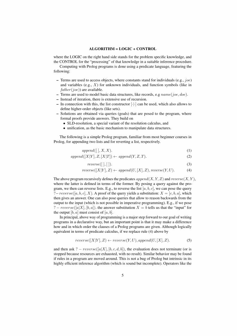
The following is a simple Prolog program, familiar from most beginner courses inProlog, for appending two lists and for reverting a list, respectively.

append([ ], X,X). (1)append([X|Y ], Z, [X|T ])← append(Y,Z, T ). (2)

reverse([ ], [ ]). (3)reverse([X|Y ], Z)← append(U, [X], Z), reverse(Y, U). (4)

The above program recursively defines the predicates append(X,Y, Z) and reverse(X,Y ),where the latter is defined in terms of the former. By posing a query against the pro-gram, we then can reverse lists. E.g., to reverse the list [a, b, c], we can pose the query?− reverse([a, b, c], X). A proof of the query yields a substitution: X = [c, b, a], whichthen gives an answer. One can also pose queries that allow to reason backwards from theoutput to the input (which is not possible in imperative programming). E.g., if we pose? − reverse([a|X], [b, a]). the answer substitution X = b tells us that the “input” forthe output [b, a] must consist of [a, b].

In principal, above way of programming is a major step forward to our goal of writingprograms in a declarative way, but an important point is that it may make a differencehow and in which order the clauses of a Prolog programs are given. Although logicallyequivalent in terms of predicate calculus, if we replace rule (4) above by

reverse([X|Y ], Z)← reverse(Y, U), append(U, [X], Z). (5)

and then ask ? − reverse([a|X], [b, c, d, b]), the evaluation does not terminate (or isstopped because resources are exhausted, with no result). Similar behavior may be foundif rules in a program are moved around. This is not a bug of Prolog but intrinsic in itshighly efficient inference algorithm (which is sound but incomplete). Operators like the

5

cut (which allow to prune the search space further, at the risk of losing solutions if doneimproperly), allow the fine control of the evaluation algorithm.

This example raises the legitimate question whether programming in Prolog is trulydeclarative. In fact, if one keeps in mind the goal of having specifications in which aproblem is declared, without knowledge on how this declaration will be processed, it isdesirable, as far as termination and finding of a solution is concerned, that

– the order of program rules does not matter, and that– the order of subgoals in a rule body does not matter.

This calls for “pure” declarative programming, in which we (possibly) trade the effi-ciency of problem solving for strict declarativity of the formalism. The major exponentof this “pure” declarative programming paradigm is the stable model semantics of logicprograms, which will be introduced in the sections below.

The stable model semantics is often confused with ASP. Indeed the semantics of thelatter has been specified in terms of the former in the seminal paper [11].

The success of ASP is based on the easy usage of ASP as a modeling language,and on the variety of sophisticated algorithms and techniques for evaluating A-Prologprograms, which originated from research on computational complexity of reasoningtasks for such programs. The complexity of ASP reasoning is well understood, and adetailed picture of it and its major extensions can be found in [12]. Advanced AS solverssuch as Smodels, DLV, GnT, Cmodels, Clasp, or ASSAT (see [13]), are able to deal withlarge problem instances; demonstration efforts of the potential of ASP are made at theAS solver competition [14] which takes place at the International Conference on LogicProgramming and Nonmonotonic Reasoning (LPNMR) since 2007.

1.3 Structure of the Article

The rest of this article is divided into three parts as follows. The first part introducesthe stable models semantics of normal logic programs and the answer set semantics ofextended logic programs, as well as of extensions thereof. Concepts and notions aregiven following a historical timeline, which incidentally coincides with the developmentof increasingly expressive specification languages based on rules. We first recall the leastmodel semantics of Horn logic programming (Section 2) and then turn to the issue ofnegation in logic programs (Section 3). Then, we consider stratified logic programs, forwhich the perfect model semantics is the canonical semantics (Section 3.1). We thenpresent the stable model semantics of normal logic programs (Section 4) which coincideswith the perfect model semantics on stratified programs (and thus generalizes it). Afterthat, we proceed with some extensions in Section 5; in particular, with constraints, withstrong negation—where we arrive at the notion of answer sets—and with disjunctiverule heads.

The second part then considers the ASP paradigm itself. It describes the general ideaand shows some ASP programming techniques (Section 6). Furthermore, it overviewsAS solvers and their general architecture and implementation principles (Section 7); asan example, we briefly present the AS solver DLV.

6

The third part is devoted to ASP in the context of the Semantic Web, presentingsome formalisms and mentioning some applications in this area (Section 8). The articleconcludes with issues of current and future ASP research.6

2 Horn Logic Programming

We will consider logic programs built from simple constituent blocks, which correspondsyntactically to the language of predicate calculus. We will have constants, whichrepresent individuals of the domain of discourse, like sarah , chicago, and 2. They willbe represented with lowercase starting letter, or with natural numbers. Variables, likeX , City , Name, denote an individual variable, and are written with uppercase startingletter. Also, one might form functional terms combining constants, functions symbolsand variables such as in next(a, Y ), where next is a binary function symbol.

In some sense, variables and constants can be seen as subjects and objects participat-ing to the scenario we are modeling, which can be tied together through predicates, likehasName and link . Predicates relate with variables and constants through atoms, likelink(chicago, paris) or hasName(C, sarah). Note that the former atom has no vari-ables in it (it is ground), while the latter is nonground. Functional terms are syntacticallyequivalent to atoms, yet they have different meaning. A (ground) atom is connected toits truth value and acts as a propositional variable: for instance, hub(rome) might betrue or false in the sense that rome might be a hub or not; on the other hand, father(gb),when seen as a functional term, denotes an individual of our domain of discourse (“thefather of gb”), for which truth or falsity makes no sense in general.

On top of these simple notions we use the idea of rules. Rules are grouped in setsthat we will call (logic) programs.

We will start with a class of logic programs featuring the simplest form of a rule.

2.1 Positive Logic Programs

Definition 1 (Positive Logic Program). A positive logic program P is a finite set ofclauses (rules) in the form

a← b1, . . . , bm , (6)

where a, b1, . . . , bm are atoms of a first-order language L. We call a the head of the rule,while b1, . . . , bm represents the rule’s body. A fact is a rule with empty body such asa←, denoted for short as a.

To give an intuition of the meaning of a rule, a reader familiar with imperative pro-gramming languages might interpret this construct as an abstraction of the if . . . then . . .construct common in traditional programming languages, to which, as it has been illus-trated, Modus Ponens might apply. For a reader familiar with first order logic, rules canbe seen as material implications restricted to Horn clauses, where A ← B is read asB ⊃ A or B → A.

6 The accompanying slides are available at http://www.kr.tuwien.ac.at/staff/tkren/pub/2009/rw2009-lecture.zip.

7

For instance, the rule

connected(cagliari)← hub(rome), link(rome, cagliari)

might be “procedurally” read as “if Rome is a hub, and there is a link between Romeand Cagliari, then Cagliari is a connected airport,” or, when seen as a first-order Hornclause in predicate logic, the same rule can be interpreted as “in any possible scenario inwhich Rome is a hub and there is a link between Rome and Cagliari, it is the case thatCagliari is connected.”

However, we will observe later that rules in declarative logic programming do notstrictly correspond to the procedural scheme of imperative languages, nor to materialimplication. Nevertheless, they are declarative constructs, and we make this more clearlater in this section.

The above example rule is ground, but logic programs might contain nongroundrules like

connected(X)← hub(Y ), link(Y,X) ,

which can be read as the universally quantified clause ∀X,Y hub(Y ) ∧ link(Y,X) ⊃connected(X). Importantly, one must distinguish between the imperative and logicalreading of clauses: a variable X in imperative programming associates a single valueto it and stands for a named storage cell, whereas X reads as “any X having a certainproperty” in the logical interpretation of clauses.

We can also think of a logic program as a description of a scenario, in which certainassertions, either specific and related to certain individuals (that is, ground), or general(that is, nonground, or partially ground), must hold.

The following definitions clarify this intuition.

Definition 2 (Herbrand Universe, Base, Interpretation). Given a logic program P ,the Herbrand universe of P , HU (P ) , is the set of all terms which can be formed fromconstants and functions symbols in P (resp. the vocabulary of L, if explicitly known).

The Herbrand base of P , HB(P ), is the set of all ground atoms which can be formedfrom predicates occurring in P and the terms in HU (P ). A (Herbrand) interpretation isan interpretation I over HU (P ), that is, I as subset of HB(P ).

An interpretation can be seen as a set denoting which ground atoms are true in agiven scenario.

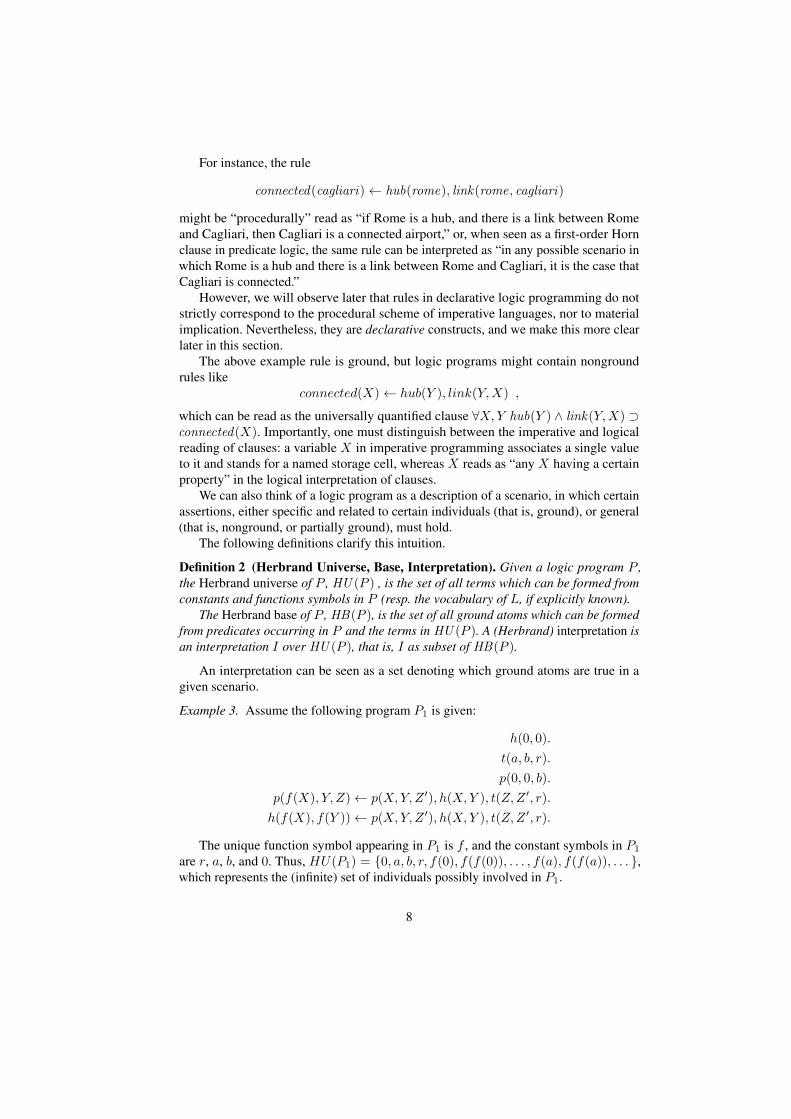
Example 3. Assume the following program P1 is given:

h(0, 0).

t(a, b, r).

p(0, 0, b).

p(f(X), Y, Z)← p(X,Y, Z ′), h(X,Y ), t(Z,Z ′, r).

h(f(X), f(Y ))← p(X,Y, Z ′), h(X,Y ), t(Z,Z ′, r).

The unique function symbol appearing in P1 is f , and the constant symbols in P1

are r, a, b, and 0. Thus, HU(P1) = {0, a, b, r, f(0), f(f(0)), . . . , f(a), f(f(a)), . . . },which represents the (infinite) set of individuals possibly involved in P1.

8

The Herbrand base is HB(P1) = {p(0, 0, 0), p(a, a, a), . . . , h(0, 0), . . . , t(0, 0, 0),t(a, a, a), . . .}, and represents the set of all possible ground assertions which might hold.

Some possible Herbrand interpretations are

– I1 = ∅,– I2 = HB(P1),– I3 = {h(0, 0), t(a, b, r), p(0, 0, b)},

and so on. An interesting question is which scenarios (interpretations) are compatiblewith P1. For instance, the interpretation {h(0, 0), t(a, b, r)} is contradicting P1, whichfollows from the simple expectation that, in virtue of the last fact in P1, also p(0, 0, b)should be considered true.

Definition 3. A ground instance of a clause C of the form (6) is any clause C ′ obtainedfrom C by applying a substitution

θ : Var(C)→ HU (P )

to the variables in C, denoted as Var(C). For any clause C, we denote by grnd(C) theset of all possible ground instances of C, and for any program P we let grnd(P ) =⋃C∈P grnd(C) (called the grounding of P ).

Intuitively, grnd(C) allows for the materialization of the universal quantification ofvariables appearing in C. Roughly speaking, C is a shortcut denoting a set of clausesgrnd(C). The range of each variable appearing inC is given by the set of terms appearingin the Herbrand universe.

Example 4. Consider the following program P2:

p(f(X), Y, Z)← p(X,Y, Z ′), h(X,Y ), t(Z,Z ′, r).

h(0, 0).

The ground instances of the first rule in P2 are

p(f(0), 0, 0)← p(0, 0, 0), h(0, 0), t(0, 0, r).

...p(f(0), r, 0)← p(0, r, 0), h(0, r), t(0, 0, r).

...p(f(r), r, r)← p(r, r, r), h(r, r), t(r, r, r).

7

Definition 4. Let I be an interpretation. Then I is a model of

7 Note that in practice most of the ground rules appearing in grnd(C) for given C might have noactual impact when computing the least model of C as defined next.

9

– a ground (variable-free) clause C = a ← b1, . . . , bm, denoted I |= C, if either{b1, . . . , bm} * I or a ∈ I;

– a clause C, denoted I |= C, if I |= C ′ for every C ′ ∈ grnd(C);– a program P , denoted I |= P , if I |= C for every clause C ∈ P .

Intuitively, a model of P is an interpretation which is compatible with assertionsappearing in P .

Example 5. Reconsider the program P2 in Example 4. Note that I1 = ∅ is not a modelof P2 (the fact h(0, 0) is not true in I1), while I2 = HB(P2) is a model; indeed,for every program P it clearly holds that HB(P ) is a model of P . However, I3 ={h(0, 0), t(0, 0, r), p(0, 0, 0)} is not a model of P2, since the first rule would requirep(f(0), 0, 0) ∈ I3.

2.2 Minimal Model Semantics

In general, there are multiple “compatible” interpretations of a program P , that is, therecan be multiple interpretations, which are models of P . Some of them are howevertrivial, e.g., think of I2 in the previous example w.r.t. P2, or they convey informationwhich is not encoded in P2. For instance, I4 = I3 ∪ {p(f(0), 0, 0), h(r, r)} is a modelof P2. There is however no evidence that h(r, r) should be true according to P2: indeedwe might remove it from I4, obtaining a smaller model I5 = I3 ∪ {p(f(0), 0, 0)}.

On the other hand, we cannot remove p(f(0), 0, 0) from I5 since the first rule of theprogram would not be satisfied. In other words, p(f(0), 0, 0) is an atom which has to benecessarily true in the scenario described by P2, while this is not the case for h(r, r).

One might ask at this point whether there exists a particular canonical model for aprogram which contains only the atoms which are necessarily true according to P . Thisnotion of “necessity” is commonly called foundedness.

Example 6. Consider the small program P3

a← b. b← c. c.

The truth of atom a in the model I = {a, b, c} is “founded.” Intuitively, c must appear inany model of P3, which implies that also b and then a are necessarily true.

Given the program P4

a← b. b← a. c.

we obtain that the truth of atom a in model I = {a, b, c} is not founded. In other words,there is no necessity of a appearing in a model. Indeed, I ′ = {c} is also a model.

The above intuition can be translated into a formal semantics, which prefers modelshaving as few true facts as is possible.

Definition 5. A model I of a program P is minimal, if there exists no model J of Psuch that J ⊂ I .

Theorem 1. Every positive logic program P has a single minimal model (called theleast model), denoted LM (P ).

10

This is entailed by the following property:

Proposition 1. If I and J are models of P , then also I ∩ J is a model of P .

Example 7. For P3 = {a ← b. b ← c. c.}, we have LM (P3) = {a, b, c}. ForP4 = {a← b. b← a. c.}, we get the least model LM (P4) = {c}

For program P1 above, we have

LM (P1) = {h(0, 0), t(a, b, r), p(0, 0, b), p(f(0), 0, a), h(f(0), f(0))} .

Computation of the Least Model. A natural question is, how we can compute the leastmodel LM (P ) of a program P .

By means of the immediate consequence operator, one can obtain LM (P ) throughan iterative process. Let TP : 2HB(P ) → 2HB(P ) be an operator defined as

TP (I) =

{a

∣∣∣∣ there exists some a← b1, . . . , bmin grnd(P ) such that {b1, . . . , bm} ⊆ I

}.

We define T 0P = ∅, and T i+1

P = TP (T iP ) for i ≥ 0.

Theorem 2. TP has a least fixpoint, lfp(TP ), and the sequence 〈T iP 〉, i ≥ 0, convergesto it, i.e., lfp(TP ) = LM (P ).

The above result can be proved by means of the fixpoint theorems of Knaster-Tarskiand of Kleene given in Appendix B. The second part of the theorem is easily shown byobserving that lfp(TP ) is a model of P and no smaller model exists.

Example 8. The immediate consequence operator captures the idea that if all the atomsin a rule r body are founded, then also the head of r must be founded.

For instance, for P3 = {a← b. b← c. c.}, we have

T 0P3

= {}, T 1P3

= {c}, T 2P3

= {c, b}, T 3P3

= {c, b, a}, T 4P3

= T 3P3

.

Hence, lfp(TP3) = {c, b, a}. For P4 = {a← b. b← a. c.}, we have

T 0P4

= {}, T 1P4

= {c}, T 2P4

= T 1P4

.

Hence lfp(TP4) = {c}.

For program P1 above, we have

T 0P1

= ∅,T 1P1

= {h(0, 0), t(a, b, r), p(0, 0, b)}T 2P1

= {h(0, 0), t(a, b, r), p(0, 0, b), p(f(0), 0, a), h(f(0), f(0))}T 3P1

= T 2P1.

11

3 Negation in Logic Programs

Positive logic programs allow for declarative modeling of a variety of problems. However,it turns out that many situations require a construct which model the intuitive notion ofnegation. Negation is a natural linguistic concept and happens to be extensively requiredwhen natural problems have to be modeled declaratively. For instance, given the rule

connected(X)← hub(Y ), link(Y,X) ,

which defines airports connected to at least one hub airport, one might think of definingairports which are not connected to any hub. This can be modeled intuitively by put thenot modifier in front of atoms, and considering the rule

badlyConnected(X)← not connected(X) .

We will define normal logic programs as a set of clauses having the form

a← b1, . . . , bm,not c1, . . . ,not cn (n,m ≥ 0) (7)

where a and all bi, cj are atoms in a first-order language L. Note that rule bodies nowinclude expressions which we call (default) negated literals not c1, . . . ,not cl, whichconsist of atoms ci preceded by the negation modifier not. Accordingly, the atomsb1, . . . , bk are called positive literals.

Intuitively, a ground literal corresponds to a propositional variable as it was the casefor atoms: a negated literal has a truth value which is opposite to its correspondingpositive literal. For instance, if hub(rome) is true, then not hub(rome) is false.

Once negated literals are syntactically defined, one can think of a proper formalmeaning for rules in which they appear. The Prolog semantics has been pragmaticallyand operationally extended from SLD to SLDNF in terms of Negation as failure: here,one considers as false a negated literal not a(·), if the truth of its corresponding positiveliteral cannot be (finitely) proved through SLD resolution.

It is important to observe that negation in classical logic is different from negation inlogic programming (cf. surveys [15, 16] and [17, 18] for more discussion).

Example 9. Consider the program P5:

man(dilbert).

single(X)← man(X),not husband(X).

husband(X)← fail . % fail = ”false” in Prolog

Under Prolog semantics, if we ask the query

?− single(X).

we obtain as an answerX = dilbert .

Intuitively, the answer is motivated by the fact that husband(dilbert) cannot be provedfrom P5. For proving single(dilbert) using forward chaining, one can use the first rule of

12

the program, in which it must be first shown that man(dilbert) holds, and then that thereis no proof for husband(dilbert); indeed, there is no evidence that husband(dilbert) istrue in P5.

Note however that this operational approach fails to give a satisfactory answer forprograms like P6

man(dilbert).

single(X)← man(X),not husband(X).

husband(X)← man(X),not single(X).

where single(dilbert) and husband(dilbert) are mutually dependent using negation.An SLD resolution algorithm would loop forever when trying to answer the querysingle(X).

Approaches which give meaning to logic programs via a model theoretic definition(that is, providing an appropriate notion for a “best” model) are able to treat recursivedefinitions for positive programs properly, for which a unique minimal model exists.However, P6 has two minimal Herbrand models

M1 = {man(dilbert), single(dilbert)}, andM2 = {man(dilbert), husband(dilbert)} .

Both M1 and M2 satisfy P6 and constitute a minimal set of necessarily true facts whichare compatible with P6. One thus may guess that introducing negation in logic programsinduces a major problem regarding the meaning of normal logic programs.

The debate about the proper semantics for attributing meaning to negation in logicprograms has been long lasting,8 and provoked what we could call the Great LogicProgramming Schism. Indeed, there are two philosophically very different approaches:

1. To keep the idea of defining a single model for a program, possibly including alsoproblematic classes of programs with negation. This can be achieved by properlydefining which single model should be selected among all classical models of aprogram. This line of research produced the notion of perfect model [21] which hasbeen agreed being satisfactory for the class of so-called “stratified programs.” Forgeneral normal problems, the most popular semantics is perhaps the one based onthe well-founded model [22].

2. To identify a collection of multiple preferred models. This line of research abandonsthe “dogmatic” requirement of a single model and accepts the possibility of havingmultiple scenarios compatible with a given program. Note that, in general, for suchmultiple models approaches, we have a single model for positive and stratifiedprograms which corresponds to the least and perfect model, respectively.

Answer Set Programming and its underlying stable model semantics is based on thelatter methodology.

8 The interested reader might refer to [15, 19, 20] for surveys about the matter.

13

3.1 Stratified Negation

As a first class of programs with negation we will consider stratified programs [23].Stratified programs have the property that one can find an ordering for the evaluation ofthe rules in the program, such that the value of negative literals can be predetermined.

Intuitively, for evaluating the body of a rule containing not r(t), the value of thenegative literal r(t) should be known. This mimics the negation-as-failure approach asfollows:

1. First evaluate r(t);2. if r(t) is false, then not r(t) is true;3. if r(t) is true, then not r(t) is false and the rule is not applicable.

Example 10. We can evaluate the single rule program

boring(chess)← not interesting(chess)

according to this recipe: as interesting(chess) clearly evaluates to false, the negatedliteral not interesting(chess) evaluates to true; hence, also boring(chess) evaluatesto true. This results in the Herbrand model H = {boring(chess)} of P , which is theintuitive meaning of P .

Note however that this implicitly introduces a particular order of evaluation for rulesand make specifications procedural more than declarative.

Dependency Graph. The above method makes only sense if there is no cyclic negationin programs. Otherwise, it is not possible to find an “evaluation ordering” for a program.The notion of dependency graph of programs captures this intuition.

Definition 6 (Dependency graph). The dependency graph of a program P , dep(P ) =〈V,E〉, consists of

– a set of nodes V , which is defined as the set of all predicates p occurring in P , and– a set of arcs E, which contains arcs of form p → q if and only if an atom with

predicate name p is in the head of a rule r ∈ P and the body of r contains a literalwith predicate name q. If this literal is under negation, the edge will be marked with? (p→? q).

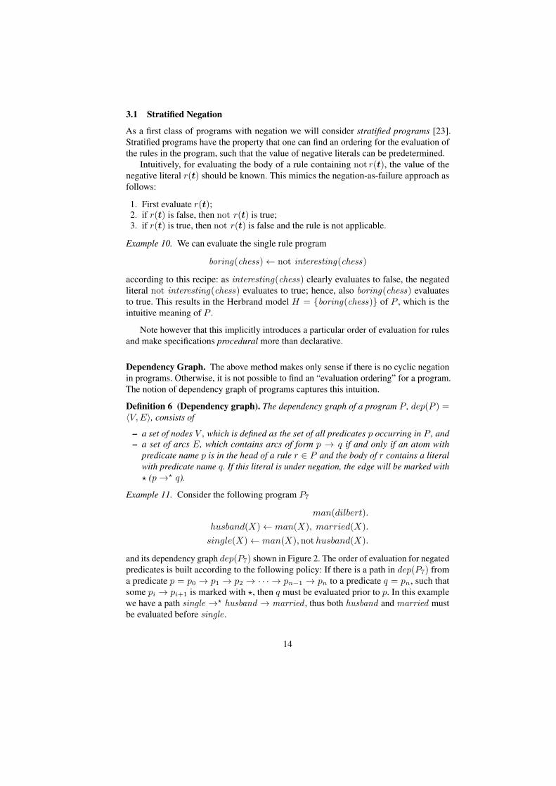
Example 11. Consider the following program P7

man(dilbert).

husband(X)← man(X), married(X).

single(X)← man(X),nothusband(X).

and its dependency graph dep(P7) shown in Figure 2. The order of evaluation for negatedpredicates is built according to the following policy: If there is a path in dep(P7) froma predicate p = p0 → p1 → p2 → · · · → pn−1 → pn to a predicate q = pn, such thatsome pi → pi+1 is marked with ?, then q must be evaluated prior to p. In this examplewe have a path single →? husband → married , thus both husband and married mustbe evaluated before single .

14

husband //

&&

married

single //

?

OO

man

Fig. 2. dep(P7)

Stratification. We formalize the notion of stratification as follows. Let pred(R) denotethe set of predicate names occurring in a set of rules R.

Definition 7 (Stratification). A stratification of a set of rules P is a partitioning Σ ={Si | i ∈ {1, . . . , n}} of pred(P ) into n nonempty and pairwise disjoint sets of predicatenames such that

(a) if p ∈ Si, q ∈ Sj , and p→ q is in dep(P ) then i ≥ j; and(b) if p ∈ Si, q ∈ Sj , and p→? q is in dep(P ) then i > j.

The sets S1, . . . , Sn are called the strata of P w.r.t. Σ. A program P is called stratified,if it has some stratification Σ.

Note that there are programs which are not stratified, such as P6 above. The strat-ification Σ specifies an evaluation order for the predicates in a logic program. Hereevaluation of a predicate p means to compute the set of true atoms that have p as pred-icate name. This sequential evaluation can be done by computing a series of iterativeleast models.

Definition 8. Let P a logic program with a stratification Σ = {S1, . . . , Sk} of lengthk ≥ 1. We define PSi as the subset of the rules of P which have a head atom whosepredicate belongs to Si, and HB?(PSi

) =⋃j≤i{p(t) ∈ HB(P ) | p ∈ Sj}. We define

the iterative least models Mi ⊆ HB(P ) with i ∈ {1, . . . , k} by:

(i) M1 is the least model of PS1;

(ii) if i > 1, then Mi is the least subset M of HB(P ) such that (a) M is a modelof PSi

, and (b) M ∩HB?(PSi−1) = Mi−1 ∩HB?(PSi−1

).

We denote by MP,Σ the iterative least model Mk.

Example 12. Consider again the program P7:

man(dilbert).

husband(X)← man(X), married(X).

single(X)← man(X), not husband(X).

According to the dependency graph dep(P7), a stratification Σ for P7 is

S1 = {man,married}, S2 = {husband}, S3 = {single} .

15

mamuk

clote

semel

quincy

olfe

ter

bis

dalte

quatericsi

Fig. 3. An example railroad network

We obtain M1 = LM (PS1) = {man(dilbert)} from the evaluation of PS1

={man(dilbert)}. When evaluating M2 we obtain

PS2= {husband(X)← man(X),married(X)} .

Note that HB?(PS1) = {man(dilbert),married(dilbert)}. It is easy to see that M2 ={man(dilbert)} is a model for PS2 , and that M2∩HB?(PS1) = M1∩HB?(PS1); also,M2 is the least model having these properties.

For the evaluation of M3, note that

PS3= {single(X)← man(X), not husband(X)} .

Thus one finds that M3 = {single(dilbert)} ∪M2 is the least model of PS3 such thatM3 ∩HB?(PS2) = M2 ∩HB?(PS2).

It is worth noting that stratifications are not unique. For instance, one can com-pute the iterative least models using an alternative stratification Σ′, in which S1 ={man,married , husband} and S2 = {single}.

In both cases the iterative least model obtained at the last iteration is the same. Animportant result tells us that, provided a stratification exists, other stratifications producethe same final model.

Theorem 3 ([23]). Let P be a stratified program. Then for every stratifications Σ andΣ′ of P , it holds that MP,Σ = MP,Σ′ .

Hence, we can drop the dependency of MP,Σ on a given stratification Σ and defineMP = MP,Σ (for a Σ of choice) as the canonical model for P , which is referred to asperfect model [21].9

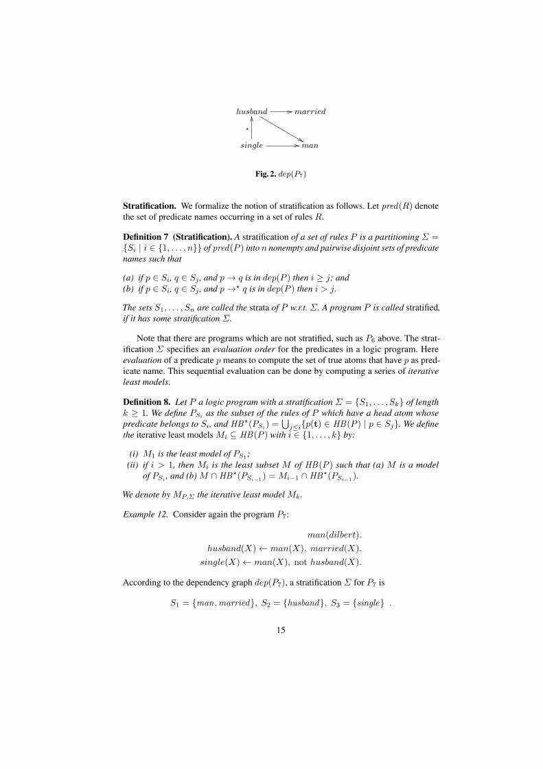
Example 13 (Railroad network). Take, as an example, the railroad network given inFigure 3. The goal is to determine whether safe connections between locations arepossible. Given two railroad stations a and b, a cutpoint station c for a and b is such thatif connections to c fail, there is no alternative connection between a and b. We will saythat the connection between a and b is safe if there are no cutpoints between a and b. InFigure 3, ter is a cutpoint for olfe and semel , while quincy is not.

The above problem can be modeled as follows. First, we introduce the set of predi-cates:

9 In fact, Przymusinski and Apt et al. developed their semantics independently, but the proposalscoincide on stratified programs, and the name perfect model for MP is customary.

16

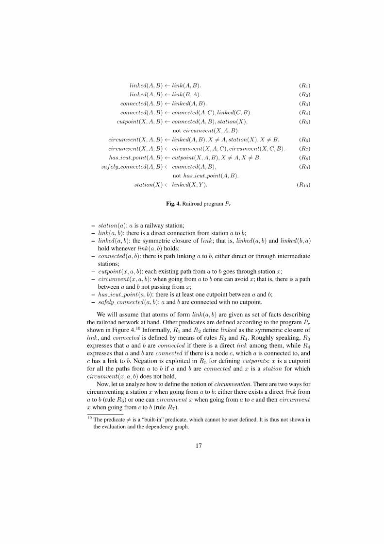
linked(A,B)← link(A,B). (R1)

linked(A,B)← link(B,A). (R2)

connected(A,B)← linked(A,B). (R3)

connected(A,B)← connected(A,C), linked(C,B). (R4)

cutpoint(X,A,B)← connected(A,B), station(X), (R5)

not circumvent(X,A,B).

circumvent(X,A,B)← linked(A,B), X 6= A, station(X), X 6= B. (R6)

circumvent(X,A,B)← circumvent(X,A,C), circumvent(X,C,B). (R7)

has icut point(A,B)← cutpoint(X,A,B), X 6= A,X 6= B. (R8)

safely connected(A,B)← connected(A,B), (R9)

not has icut point(A,B).

station(X)← linked(X,Y ). (R10)

Fig. 4. Railroad program Pr

– station(a): a is a railway station;– link(a, b): there is a direct connection from station a to b;– linked(a, b): the symmetric closure of link; that is, linked(a, b) and linked(b, a)

hold whenever link(a, b) holds;– connected(a, b): there is path linking a to b, either direct or through intermediate

stations;– cutpoint(x, a, b): each existing path from a to b goes through station x;– circumvent(x, a, b): when going from a to b one can avoid x; that is, there is a path

between a and b not passing from x;– has icut point(a, b): there is at least one cutpoint between a and b;– safely connected(a, b): a and b are connected with no cutpoint.

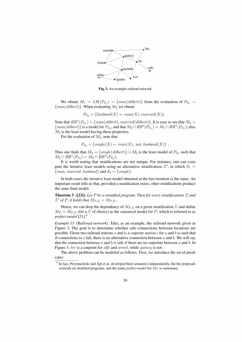
We will assume that atoms of form link(a, b) are given as set of facts describingthe railroad network at hand. Other predicates are defined according to the program Prshown in Figure 4.10 Informally, R1 and R2 define linked as the symmetric closure oflink , and connected is defined by means of rules R3 and R4. Roughly speaking, R3

expresses that a and b are connected if there is a direct link among them, while R4

expresses that a and b are connected if there is a node c, which a is connected to, andc has a link to b. Negation is exploited in R5 for defining cutpoints: x is a cutpointfor all the paths from a to b if a and b are connected and x is a station for whichcircumvent(x, a, b) does not hold.

Now, let us analyze how to define the notion of circumvention. There are two ways forcircumventing a station x when going from a to b: either there exists a direct link froma to b (rule R6) or one can circumvent x when going from a to c and then circumventx when going from c to b (rule R7).10 The predicate 6= is a “built-in” predicate, which cannot be user defined. It is thus not shown in

the evaluation and the dependency graph.

17

station -- linked

��circumvent

::

��link

has icut point // cutpoint

?

OO

]]

// connected

OO

OO

safely connected?

ee ;;

Fig. 5. Dependency graph dep(Pr) of the railroad program Pr

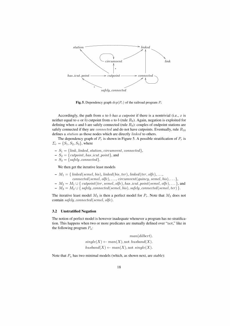
Accordingly, the path from a to b has a cutpoint if there is a nontrivial (i.e., x isneither equal to a or b) cutpoint from a to b (rule R9). Again, negation is exploited fordefining when a and b are safely connected (rule R9): couples of endpoint stations aresafely connected if they are connected and do not have cutpoints. Eventually, rule R10

defines a station as those nodes which are directly linked to others.The dependency graph of Pr is shown in Figure 5. A possible stratification of Pr is

Σr = {S1, S2, S3}, where

– S1 = {link , linked , station, circumvent , connected},– S2 = {cutpoint , has icut point}, and– S3 = {safely connected}.

We then get the iterative least models

– M1 = { linked(semel , bis), linked(bis, ter), linked(ter , olfe), . . . ,connected(semel , olfe), . . . , circumvent(quincy , semel , bis), . . . },

– M2 = M1 ∪ { cutpoint(ter , semel , olfe), has icut point(semel , olfe), . . . }, and– M3 = M2 ∪ { safely connected(semel , bis), safely connected(semel , ter) }.

The iterative least model M3 is then a perfect model for Pr. Note that M3 does notcontain safely connected(semel , olfe).

3.2 Unstratified Negation

The notion of perfect model is however inadequate whenever a program has no stratifica-tion. This happens when two or more predicates are mutually defined over “not,” like inthe following program Pu:

man(dilbert).

single(X)← man(X),not husband(X).

husband(X)← man(X),not single(X).

Note that Pu has two minimal models (which, as shown next, are stable):

18

– M = {man(dilbert), single(dilbert)} and– N = {man(dilbert), husband(dilbert)};

both might be seen as “plausible” scenarios compatible with Pu.In general, we can associate to a program P a set of preferred (or plausible) models

PM (P ). In the presence of multiple plausible models, each describing a possible scenariospecified by a given program, a natural question is how to interpret and how to reconcilepossible discrepancies between models appearing in PM (P ).

One can consider this issue from two complementary points of view:

1. One point is to see P as a knowledge base, in which explicit (facts) and implicit(rules) information is stored, and wonder if a given query q (or, in general, a formula)holds. Queries can be ground (e.g., q = man(dilbert) holds if q is true w.r.t. Puaccording to some criterion), or nonground (e.g., for evaluating q = man(X) wehave to find the set of values x such that man(x) holds in Pu).In this respect, a ground query q can be answered under Cautious (Skeptical) Rea-soning, that is q evaluates to true if it is true in every model in PM (P ), or underBrave (Credulous) Reasoning, in which q is true if it is true in some preferred model.Similarly, answering a non-ground query q amounts to finding the set of all theground assignments of q which hold in any preferred model (cautious reasoning) orin some preferred model (brave reasoning).

2. Cautious and brave reasoning can be seen as a form of quantification/iteration overpreferred models, which however still depict a single scenario. In cautious reasoningthe single scenario (the set of true facts) is described by the intersection of all themodels, while in brave reasoning one considers their union, this way discarding thericher information given in PM (P ).However, each model in PM (P ) brings peculiar information: it can be seen asthe representation of a possible world compatible with P , or, in other words, asa solution to the problem instance encoded by P . Model generation (that is, thecomputation of the set PM (P )) in this respect is—more than query answering—ofvaluable importance.

Example 14. The preferred models M and N of Pu represent “possible worlds” compat-ible with Pu. The ground atom man(dilbert) is a cautious and brave consequence of Pu.But, neither single(dilbert) nor husband(dilbert) are cautious consequences, whereasboth are brave consequences of Pu (the first holds in M while the second holds in N ).

4 Stable Semantics

Many definitions for PM (P ) have been conceived in the past, cf. [15, 24]. We willconcentrate from this point on the—largely considered the most prominent one—notionof preferred model based on stable models.

4.1 Normal Logic Programs – Syntax

A logic program P based on the stable model semantics has the same syntactic buildingblocks as stratified programs: importantly, it is not necessary that P has a stratification,

19

as we do not rely on the notion of perfect model for computing its semantics. Also,we keep the the notions of Herbrand universe HU (P ), Herbrand base HB(P ), andinterpretation as for not-free (“positive”) logic programs.

4.2 Stable Model Semantics

First, we will define the stable model semantics for a variable-free (ground) program.The intuition behind stable model semantics is to treat negated atoms in a special

way. Intuitively, such atoms are a source of “contradiction” or “unstability.”

Example 15. In Pu from above, one can consider M ′ = {man(dilbert)} as possi-ble, preferred model. Assuming facts in M ′ as true, note however that the two rulesof Pu would enforce to assume that besides man(dilbert) also single(dilbert) andhusband(dilbert) are true. On the other hand, if one considers M ′′ = {man(dilbert),single(dilbert), husband(dilbert)} as the set of true facts, it turns out that the two rulesof Pu have now their bodies false, and do not give evidence of truth for single(dilbert)and husband(dilbert).

“Stability” can thus be seen as follows: if an interpretation M of P is not—in thesense formalized below—self-contradicting, then it is stable.

Definition 9. The Gelfond-Lifschitz reduct [8] (short GL-reduct or simply reduct) of aprogram P w.r.t. an interpretation M , denoted PM , is a program obtained by

1. removing rules with not a in the body for each a ∈M ; and2. removing literals not a from all other rules.

Intuitively, given an interpretation M , the conditions 1 and 2 above enforce truthvalues for negative literals. If a ∈M , then a rule’s body with the negative literal not acannot become true. On the other hand, if a /∈ M , the not a can be assumed true andremoved from any body where it occurs.

In other words, M can be seen as an assumption about which negated literals are trueand what are false; the program PM incorporates these assumptions. Note that PM is apositive program, and thus has a least model LM (PM ). If PM does not “contradict” M ,one should expect that LM (PM ) = M , that is, M can be reconstructed from scratchapplying the rules of PM . If this happens to be the case, then M can be regarded asbeing “stable.”

Definition 10. An interpretation M of P is a stable model of P , if

M = LM (PM ).

Note that PM = P for any “not”-free program P . Thus, LM (P ) (which is equal toLM(PM )) is its single stable model.

Example 16. If we take Pu again in consideration

man(dilbert). (f1)single(dilbert)← man(dilbert),not husband(dilbert). (r1)

husband(dilbert)← man(dilbert),not single(dilbert). (r2)

we may have the following “candidate” interpretations:

20

– M1 = {man(dilbert), single(dilbert)},– M2 = {man(dilbert), husband(dilbert)},– M3 = {man(dilbert), single(dilbert), husband(dilbert)}– M4 = {man(dilbert)},

One can verify that only M1 and M2 qualify themselves as stable models.

– if we consider M1 we get that the reduct PM1u is

man(dilbert).

single(dilbert)← man(dilbert).

Note that husband(dilbert) /∈ M1, thus not husband(dilbert) is removed fromr1. On the other hand r2 is deleted from Pu since single(dilbert) ∈ M1: indeed,under the assumption made in M1, the literal not husband(dilbert) is false andwill prevent r2 to trigger and make its head true.The least model of PM1

u is {man(dilbert), single(dilbert)} which coincides withM1.Symmetrically, we can verify that M2 is stable as well.

– On the other hand, M3 and M4 are not stable. If we take M3 = {man(dilbert),single(dilbert), husband(dilbert)} in consideration, we find that PM3

u consistsonly of man(dilbert). Both r1 and r2 are indeed deleted. Thus, LM (PM3

u ) ={man(dilbert)} 6= M3. This means that the assumptions made in M3 are not“stable” with respect to negated literals in Pu.If we take M4 = {man(dilbert)}, we observe that PM4

u consists of

man(dilbert).

single(dilbert)← man(dilbert).

husband(dilbert)← man(dilbert).

given that both not husband(dilbert) and not single(dilbert) are removed fromr1 and r2 respectively. Therefore, LM (PM4

u ) = {man(dilbert), single(dilbert),husband(dilbert)} 6= M4.

Notably, there are situations in which “stability” is impossible and no meaning canbe assigned to a program.

Example 17. The program Pip← not p. (8)

has no stable models. Consider any interpretation M for Pi such that p /∈ M . Thus,not p is true and the body of (8) is satisfied, which means that p should be true as wellin order for M being a model for Pi. But this is in direct contradiction to p /∈M . Now,if we take an interpretation M ′ such that p ∈ M ′, we get that not p is false and ourrule (8) is satisfied, hence M ′ is a model for Pi. But it is not a stable model, as the reductPM

′

i = ∅, and we have that LM (PM′

i ) = ∅, which is different from M ′.If we take an arbitrary program P , and add the rule (8) (with p being a new proposi-

tional atom), we get that P has no stable model.

21

Example 18. Consider the program Ps:

s← not q. (r1)q ← not s. (r2)p← q,not s. (r3)f ← s,not f. (r4)

Ps has a single stable model M1 = {p, q}, while M2 = {s} is not stable.

– Indeed, for M1 = {p, q} we have that in PM1s the rules r1 is deleted, while r2, r3

and r4 are modified, obtaining:

q.

p← q.

f ← s

For which LM (PM1i ) = {p, q} = M1.

– For M2 = {s}, we get PM2s by deleting r2 and r3 from Ps and updating r1 and r4:

s.

f ← s.

We get LM(PM2s ) = {s, f} 6= M2. Note that M3 = {s, f} is not stable as

well. Indeed, one can observe that rule r4 prevents the existence of a stable modelcontaining s.

Programs with Variables. As for the case of positive and stratified programs, it isimmediate to lift the notion of stable model from propositional programs to non-groundones. Intuitively, this step amounts to considering non-ground rules (containing variables)as shorthands for all their possible ground instances, obtained using a domain of choicefor the terms which can be constructed. This latter domain is usually the Herbranduniverse of the program at hand. The stable semantics of non-ground programs is thusobtained by means of a reduction to the variable-free case.

Definition 11. Given a program P , an interpretation M of P is a stable model of P , ifM is a stable model of grnd(P ).

Example 19. Consider the following variant of Pu which we will call Pu′ :

man(dilbert). (r1)woman(alice). (r2)

single(X)← man(X),not husband(X). (r3)husband(X)← man(X),not single(X). (r4)

22

We have that, for instance,

grnd(r3) = { single(dilbert)← man(dilbert),not husband(dilbert).

single(alice)← man(alice),not husband(alice). };

grnd(Pu′) = { man(dilbert).

woman(alice).

single(dilbert)← man(dilbert),not husband(dilbert).

single(alice)← man(alice),not husband(alice).

husband(dilbert)← man(dilbert),not single(dilbert).

husband(alice)← man(alice),not single(alice). }.

The program grnd(Pu′), and thus Pu′ , has the following stable models:

– M1 = {man(dilbert), woman(alice), single(dilbert)}– M2 = {man(dilbert), woman(alice), husband(dilbert)}

4.3 Semantic Properties of Stable Models

The success of stable models as semantics for normal logic programs (with arbitraryusage of negation) relies on two important aspects: first, stable models have a strongtheoretical basis, and enjoy many properties which reflect natural intuitions. Second,as it will be seen in Section 6 they pave the way to a innovative problem modelingmethodology.

We survey here some important (most of which desirable) theoretical properties ofstable models. The reader can refer to [25–27] for other insights, alternative definitionsand properties of stable models.

We first consider the relationship between stable models and classical models of alogic program, i.e., when negation as failure is interpreted as classical negation.

To this end, the notion of (classical) Herbrand model is easily lifted to clauses withnegated literals in their bodies.

Definition 12. Let I be an interpretation. Then I is a model of

– a ground clause C : a← b1, . . . , bm,not c1, . . . ,not cn, denoted I |= C, if either{b1, . . . , bm} * I or {a, c1, . . . , cn} ∩ I 6= ∅.

– a clause C, denoted I |= C, if I |= C ′ for every C ′ ∈ grnd(C);– a program P , denoted I |= P , if I |= C for every clause C in P .

Intuitively, the above definition lifts Definition 4 by taking in consideration negatedliterals: an interpretation I is, again, “compatible” with a clause C either if it containsthe head of C, or if the body of C is false. A body can be false either if some positive biis not in I , or if some ci is in I . One expects that if the body of C is true, then also itshead must be true: indeed, if b1, . . . , bm ∈ I and c1, . . . , cn /∈ I , I can be model of Conly if it contains a.

The above definition complies with the notion of Herbrand model satisfying theclause a ∨ not b1 ∨ . . . ∨ not bm ∨ c1 ∨ . . . ∨ cn, where not is interpreted as classicalnegation. Now the following property holds:

23

Theorem 4. 1. Every stable model M of P is a model of P .2. A stable model M does not contain any model M ′ of P properly (M ′ 6⊂M ), i.e., is

a minimal model of P (w.r.t. ⊆).

The above properties guarantee that stable models of a program with negation enjoytwo of the desirable properties holding for least models of positive programs: first, astable modelM of P is “compatible” with all the rules of P , that is, it does not contradictP . Also, M contains a minimal amount of facts which one must admit to be true forgaining the “compatibility” with the scenario described by P , and no unnecessary and/orredundant information.

Corollary 1. Stable models are incomparable w.r.t. ⊆, i.e., if M1 and M2 are differentstable models of P , then M1 *M2 and M2 *M1.

Also, stable models gracefully generalize the semantics for positive programs (theleast model of a positive program P is clearly the unique stable model of P ), and forstratified semantics: indeed, the perfect model of a stratified program is also its uniquestable model.

Theorem 5. If a program P is stratified, then P has a single stable model, whichcoincides with the perfect model.

Note, for instance, that the railroad program Pr is stratified. Its single stable modelcoincides with the perfect model. It is indeed worth noting that there is only one stableconfiguration for a stratified program although it can have multiple minimal models.

Example 20. If one considers the program Pm

p(a).

r(X)← p(X),not q(X).

we get two minimal models M1 = {p(a), r(a)} and M2 = {p(a), q(a)} for Pm. Notethat while M1 is stable, M2 is not stable, as the reduct grnd(Pm)M2 = {p(a)}, andLM (grnd(Pm)M2) = {p(a)} 6= M2.

What makes M2 different from M1 is the fact that there is neither rule nor fact inPm justifying the presence of q(a) in a model.

Indeed one can see stable models as models in which all atoms a ∈M are somehow“supported” by evidence: in a sense, a stable model “supports”, or “gives evidence” ofthe truth of each a ∈M .

Theorem 6. Given a program P and an interpretation I , let

TP (I) =

{a

∣∣∣∣ there is some r = a← b1, . . . , bm, c1, . . . ,not cn ∈ grnd(P )such that {b1, . . . , bm} ⊆ I, {c1, . . . cm} ∩ I = ∅

}.

If I is a stable model of P , then TP (I) = I .

Example 21. Note that q(a) in example 20 is unsupported in M2, indeed q(a) 6∈TP (M2).

24

Nonetheless, it must be noted that there are models which are minimal fixed pointsof TP , but are however not stable:

Example 22. Consider the short program Ps:

a← not b.

b← c.

c← b.

Note that M1 = {a} and M2 = {b, c} are both minimal and such that TPs(M1) = M1

and TPs(M2) = M2, respectively. In particular, b and c are—in a sense—self-supported.

Consider the reducts PM1s = {a ←; b ← c; c ← b} and PM2

s = {b ← c; c ← b}.We have that LM (PM1

s ) = {a} = M1 and LM (PM2s ) = ∅ 6= M2, thus M1 is a stable

model, whereas M2 is just a minimal model, but not a stable one.

Self-supported atoms are in general not desirable, since they can lead to paradoxicalscenarios in which true facts are not supported by evidence; a and b from the previousexample are indeed unfounded w.r.t M2 in the sense specified below.

Definition 13 ([22]). Given a program P , a set U ⊆ HBP is an unfounded set ofP relative to an interpretation I , if for every a ∈ U and every r ∈ ground(P ) withH(r) = a, either

1. There is some atom b appearing as positive literal in the body of r which is suchthat either b 6∈ I or b ∈ U , or

2. There is some atom b appearing as negative literal in the body of r such that b ∈ I .

For normal programs there exists the greatest unfounded set of P relative to I , denotedby UP (I).

Intuitively, if I is compatible with P , then all atoms in UP (I) can be safely switchedto false and the resulting interpretation is still compatible with P . Assuming I as a set oftrue facts, there is no rule in P that can justify an atom a ∈ U becoming true.

An interpretation I is called unfounded-free, if I ∩ U = ∅ for each unfounded set Uof P rel. to I . In other words, I is unfounded-free iff I ∩ UP (I) = {}.

11

The notion of unfounded set extends the notion of “non-supportedness” by implicitlyforbidding support of an atom by an atom which is unfounded. For gaining “foundedness”byM an atom a ∈M necessitates support by a rule whose body is made true by foundedatoms only (not belonging to the unfounded set at hand).

Theorem 7 (implicit in [28]). Given a program P , a model M of P is stable iff M isunfounded-free.

11 Note that, for more general classes of programs than normal programs (e.g., disjunctive programas later defined in Section 5.3), UP (I) is undefined. More generally, we can then say that I isunfounded-free, if there is no (non-empty) subset of I which is an unfounded set.

25

Example 23. If we take Pu again in consideration

man(dilbert). (f1)single(dilbert)← man(dilbert),not husband(dilbert). (r1)husband(dilbert)← man(dilbert),not single(dilbert). (r2)

And the four following “candidate” interpretations:

– M1 = {man(dilbert), single(dilbert)},– M2 = {man(dilbert), husband(dilbert)},– M3 = {man(dilbert), single(dilbert), husband(dilbert)}– M4 = {man(dilbert)},

One can observe thatM3 has the greatest unfounded setUPu(M3) = {single(dilbert),

husband(dilbert)}: assuming M3 as a set of “true” facts, there is indeed no rule whichcould make atoms in UPu(M3) true. M3 is thus not unfounded-free. Note that M4 is nota model at all, since r1 and r2 are not satisfied.

Example 24. Note that the minimal model M2 = {b, c} of Ps is not unfounded free:indeed UPs

(M2) = {b, c}.

Reasoning from stable models. Since a logic program P might have no, one, ormultiple stable models, the question is how inference from P should be defined. Withrespect to a particular stable model M , a ground atom a is considered to be true (denotedM |= a), if a ∈M , and false, if a /∈M . This is usually extended to inference from allstable models of P in two dual modes, as mentioned already in Section 3.2:

Brave Reasoning An atom a is a brave (or credulous) consequence of P , denotedP |=b a, if M |= a for some stable model of P ;

Cautious Reasoning An atom a is a cautious (or skeptical) consequence of P , denotedP |=c a, if M |= a for every stable model of P .

These notions can be extended to propositional combinations of ground atoms inthe natural way (where M |= ¬a iff a /∈M ), and similarly to (combinations of) closedformulas.

Both |=b and |=c are nonmonotonic, as adding further rules to P might invalidate aconclusion.

Example 25. If we reconsider the program Pm in Example 20, then both Pm |=b r(a)and Pm |=c r(a), as r(a) is true in the unique stable model of Pm. However, forP ′m = Pm ∪ {q(a)}, neither P ′m |=b r(a) nor P ′m |=c r(a) holds, as r(a) is false in thesingle stable model {p(a), q(a)} of P ′m.

From this example, one might believe that the nonmonotonic behavior of inferenceis due to the fact that we added some fact (q(a)) that was missing before, but that thiswould not happen if the fact were already a consequence; that is, that inference satisfiescautious monotonicity:

26

– If P |=x a and P |=x b, then P ∪ {a} |=x b.

where x ∈ {b, c}. This property is obviously fulfilled for classical inference |= in placeof |=x. However, it does not hold for cautious reasoning under stable semantics.

Proposition 2. In general, P |=c a and P |=c b does not imply that P ∪ {a} |=c b.

In fact, the property fails even if P has a single stable model. For example, consider theprogram P = {b← not c; c← not b; a← not a; a← b}. This program has the singlestable model M = {a, b}, and thus P |=c a and P |=c b. However, the program P ∪{a}has another stable model, viz. N = {a, c}, and thus P ∪ {a} 6|=c b. The property is,however, true for brave reasoning.

Similarly then, also the stronger property of cumulativity fails:

– If P |=x a, then P |=x b iff P ∪ {a} |=x b.

That is, by adding consequences as “lemmas,” we might change the set of conclusionsthat can be drawn (which is not the case for classical inference |=). In fact, this propertyalso fails for brave reasoning, as shown by the above examples (e.g., P ∪ {a} |=b cwhile P 6|=b c).

In conclusion, care is needed when arguing about how rules in a program computetruth values for atoms under stable semantics. As long as atoms do not depend onnegation through cycles, i.e., in the stratified part of a program, adding atoms that arecomputed true as facts does not change the semantics. Fortunately, this can be generalizedto settings where a program can be split into an “lower’ and an “upper” part where theformer informally provides input to the latter in a modular way [29]. In other cases, onehas to carefully examine the effects of adding atoms—in an unfounded way—as facts.More about properties of consequences from stable models can be found e.g. in [27].

4.4 Computational Properties

There are many computational tasks related to logic programs under stable modelsemantics: one might want to check if a given program P is consistent (that is, it admitsat least one stable model), or to compute one, or all, of its models. Also it can be ofinterest to determine truth of a given query Q under brave or cautious reasoning. Webriefly focus here on the problem CONS of deciding whether a given input programP has some stable model, that is, deciding the consistency of P under stable modelsemantics. The computational complexity of CONS has direct impact on other relatedproblems, thus giving an indication of the complexity of other related problems. Forinstance, evidence of consistency can be given by computing one stable model.

It turns out that assessing consistency of a ground program P is in general NP-complete.

Theorem 8 ([30]). The problem CONS of deciding whether a given ground program Phas some stable model is NP-complete.12

12 Recall that NP is the class of problems solvable in polynomial time on a non-deterministicTuring machine [31].

27

Intuitively, this result can be justified by thinking of a simple nondeterministic algorithmfor checking the existence of a stable model for P . For showing that CONS is in NPone can: (i) guess a candidate stable model M ; (ii) check in polynomial time if M isstable (e.g. by verifying UP (M) = {}). Also, one can show that it is possible to build aprogram Pφ, having a stable model iff a given propositional formula φ in CNF is true(where Pφ is of size at most polynomially higher than the size of φ).

However, computational complexity might change depending on allowed extensions(disjunction, presence of function symbols, etc.):

– For “not”-free programs and stratified programs, CONS can be solved in polynomialtime (in fact, solvable in linear time);

– For programs with variables but not function symbols, CONS has exponentiallyhigher complexity (NEXP-complete);

– For non-ground, arbitrary programs (allowing functional terms), CONS is unde-cidable. There are however known syntactic conditions on the usage of functionsymbols which retain complexity in 2-EXP [32, 33] resp. 2-NEXP [34, 35].13

It is important to note the dramatic change in complexity when P is non-ground. Thisshould not be surprising if one considers that, usually, grnd(P ) is exponentially biggerthan P .

Example 26. Given the rule rg

r(X1, . . . , Xk)← h(a, b), c1(X1), . . . , ck(Xk)

one can easily observe that |grnd(rg)| = O(2k).

In particular one can observe that the size of a grounded program can be exponentiallybigger than its original non-ground counterpart if k is allowed to vary, that is, if programscan have arbitrarily long rules, and arbitrarily large arities. This might not be the case ifa bound on such parameters is given (see e.g. [36]). Also, one might wonder why theintroduction of function symbols makes CONS undecidable. One can easily see that, inthis setting, it is possible to have stable models of infinite size:

Example 27. Consider the program Pf :

p(a).

p(f(X))← p(X).

We can observe that grnd(Pf ) = {p(a), p(f(a))← p(a), p(f(f(a)))← p(f(a)), . . . }is infinite, as well as its unique stable model Minf = {p(a), p(f(a)), p(f(f(a)), . . .}.It is thus not surprising that for non-ground programs, admitting functions symbols, CONSand other related reasoning problems become as difficult as deciding the termination ofa Turing machine on a given input.14

13 A decision problem is in 2EXP (2NEXP) time, if it can be solved by a (non-)deterministicTuring Machine in time O(22

p(n)

), where p(·) is a polynomial and n is the size of the inputinstance.

14 The reader can find in [12] a thorough collection of results regarding computational complexityof logic programming under various semantics including the stable models semantics.

28

5 Extensions

In the above sections, we have dealt with the motivation and history of answer setprogramming, and described syntax and semantics of gradually increasing expressiveprogram classes. In particular, we looked into the class of normal logic programs understable models semantics and showed their alluring semantic properties. But, so far, wedid not touch upon the full area of answer set programming. In this section, we willapproach the main topic of this chapter and show more syntactic extensions of normallogic programs and define their semantics, which, eventually, brings us to the answer setsemantics.

We now turn our attention to three particular extensions of normal logic programsthat lead to the notion of Answer Set Programming: (i) (integrity) constraints (rules withempty head) like

← edge(X,Y ), red(X), red(Y ) , (9)

which forces that adjacent nodes in a graph are not allowed to have the colour red;(ii) strong (or “classical”) negation in atoms, e.g., −single(dilbert) (Dilbert is knownnot to be a single); and (iii) disjunctive rules, i.e., allowing for disjunctions in rule headslike in

female(X) ∨male(X)← person(X) ,

which intuitively means that persons are either female or male. For many crucial knowl-edge representation tasks, these extensions are not only desirable, but also necessary forsuccinct encodings of problems. Programs that permit strong negation are also called Ex-tended Logic Programs (ELP). If ELPs additionally allow for disjunctive rules, we obtainthe class of disjunctive ELPs, which are also called Disjunctive Logic Programs (DLP).

Next, we will look into these important extensions in more detail and then providesyntax and semantics of ELPs and DLPs.

5.1 Constraints

Integrity constraints check admissibility of models, possibly using auxiliary predicatesdefined by normal stratified rules. For instance, the constraint rule (9) can be equallywell expressed as the “killing clause”

falsity ← not falsity , edge(X,Y ), red(X), red(Y ) , (10)

where falsity is a fresh propositional atom. Now, if there is an interpretation I for aprogram with the constraint (9) such that I contains edge(a, b), red(a), and red(b), butfalsity /∈ I , then (10) is applicable and forces falsity to be true. But then, I cannot bea model for our program, as falsity is false in I . This means that (10) “kills” all modelsthat do not satisfy the constraint (9).

5.2 Strong Negation

In Section 3, we have defined normal logic programs, i.e., logic programs that allow forweak negation in rule bodies. The intuitive meaning of not a is that “a cannot be proved

29

(derived) using rules,” and that a is false by default (or believed to be false). But this isdifferent from (provably) knowing that a is false, which is expressed by ¬a; in ASP, onealso writes −a for this.

Example 28 (by John McCarthy). Consider an agent A with the following task: “At arailroad crossing, cross the rails if no train approaches.” We may encode this scenariousing one of the following two rules:

walk ← at(A,L), crossing(L),not train approaches(L). (11)walk ← at(A,L), crossing(L),−train approaches(L). (12)

In the following, let us assume that A is at some crossing L.If we take (11) as encoding for the railroad-crossing task, and A cannot infer from

her beliefs that train approaches(L) is true, then A will conclude to walk even thoughA cannot be sure that there is no approaching train: her beliefs might not represent thestate of the world completely. Now, if we take (12) as the encoding, A will only walk ifshe can prove that there is no approaching train.

In (11), an update to A’s knowledge can lead to revised conclusions; if we addtrain approaches(L), then A will refuse to walk. This is the typical behavior of non-monotonic rules like (11), but may not be desired in critical situations like crossing arailroad, as an approaching train, which has not been perceived by A yet, might causedevastating effects on the agent. From this point of view, the rule (12) employing strongnegation is preferable.

There are several ways to express negative knowledge using strongly negated atoms.One way is to explicitly state them as facts in a knowledge base. For instance, the fact−broken(battery) expresses that a battery is definitely not broken. If this knowledgebase concludes in a different rule that broken(battery) holds, then we face inconsistency,and this causes to vanish all models of that particular knowledge base.

Another useful application for strong negation (in combination with weak negation)is to express default rules. For example, we can express that “a bird flies by default” withthe rule flies(X)← bird(X),not −flies(X).

Extended Logic Programs. Adding strong negation to normal logic programs leads tothe so called extended logic programs.

Definition 14. An extended logic program (ELP) is a finite set of rules

a← b1, . . . , bm,not c1, . . . ,not cn (n,m ≥ 0) (13)

where a and all bi, cj are atoms or strongly negated atoms in a first-order language L.

The semantics of ELPs can be defined in different ways, either genuinely by con-sidering sets of ground literals rather than sets of atoms as basis, as done in [11], or bya simple reduction to normal logic programs that compiles strong negation away; wefollow here for simplicity the latter. To this end, we

30

– view negative literals “−p(X)” as atoms with fresh predicate symbols −p, for eachatom p(X);

– add the clausefalsity ← not falsity , p(X),−p(X) (14)

to P (this prevents that p(X) and −p(X) are true at the same time); and– select the stable models of the resulting program P ′. These are called answer sets ofP .

Note that extended logic programs have similar properties as normal logic programsunder stable models semantics. For a ground atom a, constraint (14) prevents that botha and −a are contained in answer sets. One takes a three-valued view on this: an atommay be true, false, or undefined (i.e., we don’t know if the atom is true or false). Thiscontrasts with the two-valued view of stable models of a normal logic program, in whichan atom a is either true (if a is in the model) or false (if a is not on the model, in thespirit of Reiter’s Closed World Assumption [37]).15

The use of strong negation may cause inconsistency, even if a program does not haveweak negation. For example, take the program P

true.

trivial← true.

a← true.

−a← true.

which derives both a and −a. The constraint (14) prevents that P has answer sets, thusP is inconsistent. However, this inconsistency is of a different quality than the one causeby default negation (cf. Example 17).

Example 29. The next program is a knowledge base for determining if one should querythe science citation index (sci) or the citeseer database:

up(S)← website(S),not −up(S). (r1)−query(S)← −up(S). (r2)query(sci)← not −query(sci), up(sci). (r3)

query(citeseer)← not −query(citeseer),−up(sci), up(citeseer). (r4)flag error ← −up(sci), −up(citeseer). (r5)

website(sci). website(citeseer).

In rule (r1), we define that websites are up by default, and (r2) encodes that a websiteknown to be not up should not be queried. The rules (r3) and (r4) give a preference onthe websites: whenever we cannot prove that sci is not usable and sci is available, thenwe should query the science citation index, but we should only query citeseer if it isavailable for querying and sci is down. In (r5), we simply raise an error-flag wheneverboth websites are down.15 The answer sets of an ELP P without strong negation coincide with the stable models of P ,

and thus the terms are often used interchangeably (confusing two- vs three-valuedness).

31

The single answer set of this program is

M = {website(sci), website(citeseer), up(sci), up(citeseer), query(sci)} ,

whose intuitive meaning is that we should query the science citation index, even thoughciteseer is up and running.

If we add to our knowledge base the rule

−query(S)← not query(S),−reliable(S) (r6)

and the facts that sci is down and citeseer is unreliable,

−up(sci) and − reliable(citeseer) ,

we can witness a different behavior. Intuitively, (r6) creates a nondeterminism in ourprogram, as for websites S that are known to be unreliable we can infer−query(S), pro-vided that we cannot prove query(S). But rules (r3) and (r4) gives us similar knowledge,except with unlike signs: we can infer a positive fact query(S) given that we cannotprove −query(S). To resolve this conflicting views, we obtain for our knowledge baseunder answer set semantics exactly two answer sets, with each intuitively describe thecorresponding alternative view on our site selection problem:

– M1 = {website(sci), website(citeseer), −up(sci),up(citeseer),−reliable(citeseer),−query(sci), query(citeseer)}, and

– M2 = {website(sci), website(citeseer), −up(sci),up(citeseer), −reliable(citeseer), −query(sci), −query(citeseer)},

i.e., in M1 we have chosen to query citeseer and in M2 we conclude that we should notquery citeseer, thus querying no website at all.

Relationship to Reiter’s Default Logic. It has been noted already in [11] that ELPs areclosely related to Reiter’s famous Default Logic [38]. For an ELP clause C of form (13),consider the corresponding default

d(C) =b1 ∧ · · · ∧ bm : ¬.c1, . . . , ¬.cn

a,

where ¬.ci is the opposite of ci (i.e., ¬.a = ¬a and ¬.¬a = a).

Theorem 9. Let P be an extended logic program and let T = (∅, {d(C) | C ∈ P})be the corresponding default theory. Then, M is an answer set of P if and only ifE = Cn(M) is a consistent default extension of T .

Thus, extended logic programs under answer set semantics can be regarded as afragment of default logic.

32

5.3 Disjunction

The next extension to normal logic programs is disjunctions in rule heads. The use ofdisjunction is natural to express indefinite knowledge. For instance, the rule

female(X) ∨male(X)← person(X)

expresses that all persons are either female or male. Another example is the disjunctivefact

broken(left hand , tom) ∨ broken(right hand , tom)← ,

which expresses that tom has a broken arm, but it is unknown whether the left or theright hand is broken.

Disjunctive information is a natural extension for expressing a “guess” and to createnon-determinism in logic programs, like in the rule

ok(C) ∨ −ok(C)← component(C) ,

which states that a component may be in a working condition or not working at all, andin each of the alternative states of the component, we might have to take different actionsfor solving our problem.

The semantics of disjunctive rules is such that we conclude one of the alternatives tobe true (the minimality principle).

In the next example, we look at different disjunctive programs, and the models theyadmit.

Example 30. Disjunction is minimal, i.e., from a rule, we usually infer only a singleatom “at a time.” The single rule program

a ∨ b ∨ c← (15)

has three minimal models: {a}, {b}, and {c}. There exist no smaller models for (15),since ∅ is not a model. The interpretation I = {a, b} for instance is a model of thisprogram, but both {a} and {b} are smaller than I and satisfy (15), hence I is not aminimal model.

If we take a closer look into the minimal models of disjunctive programs, we observethat they are actually subset minimal. Take, for instance, the program

a ∨ b← (16)a ∨ c← (17)

This program has two minimal models: {a} and {b, c}. The interpretation J = {a, b, c}is a model for both (16) and (17), hence it is a model of the program. But J is a propersuperset of {b, c}, thus J is not a minimal model. Note that {a} is the only singletonminimal model, as both {b} and {c} do not satisfy the program.

In a similar vein, the program

a ∨ b← (18)a← b (19)

33

has the single minimal model {a}, as the model {a, b} is not minimal with respect toset inclusion. The interpretation {b} is not a model; it satisfies rule (18), but it is not amodel for (19).

Note that disjunction should not be understood as exclusive. Take program

a ∨ b← (20)b ∨ c← (21)a ∨ c← (22)

which has three minimal models {a, b}, {a, c}, and {b, c}. Each of the three minimalmodels are not contained in the other, but the intersection of any two of the minimalmodels is nonempty.

Let us next consider the use for disjunctive rules vs. unstratified negation. Goingback to our Dilbert scenario, the program

man(dilbert). (23)single(X)← man(X),not husband(X). (24)husband(X)← man(X),not single(X). (25)

which expresses that a man is either a single or a husband, is equivalent to the disjunctiveprogram

man(dilbert). (26)single(X) ∨ husband(X)← man(X). (27)

Here, the use of disjunction is more intuitive. In fact, one can see the rule (27) re-sulting from (24) resp. (25) by “shifting” the negated literal not husband(X) (resp.not single(X)) to the head (classically, the clauses are equivalent). While such shiftingworks in this example, as well as under certain syntactic conditions (like headcycle-freeness) [39], we note that in general, disjunctive rule heads are not syntactic sugar forunstratified negation; this is also evidenced by complexity results provided in Section 5.3.

Extended Logic Programs with Disjunctions. The extension of ELPs with disjunctiverule heads leads to the class of extended disjunctive logic programs in [11].

Definition 15. A extended disjunctive logic program (EDLP) is a finite set of rules

a1 ∨ · · · ∨ ak ← b1, . . . , bm,not c1, . . . ,not cn (k,m, n ≥ 0)

where all ai, bj , and cl are atoms or strongly negated atoms.

The semantics for an EDLP can be defined similarly as for an extended logic program,with the only difference being that instead of choosing a stable model M of P (i.e., Mis the least model of the reduct PM ), we define an answer set M of an EDLP P as aminimal model M of the reduct PM , since multiple minimal models of PM might exist.

34

Example 31. Consider the program P :

man(dilbert).

single(X) ∨ husband(X)← man(X).

There are two answer sets for P :

– M1 = {man(dilbert), single(dilbert)}, and– M2 = {man(dilbert), husband(dilbert)}.

Please note that P is “not”-free (positive), hence the reduct grnd(P )M = grnd(P )for every interpretation M .

It is worth mentioning here that answer sets of EDLPs can also be nicely definedin equilibrium logic [40, 41], which is a non-monotonic version of the logic of hereand there, an intermediate logic between classical logic and intuitionistic logic. Thislogic is well-suited to capture not only EDLPs, but also other extensions of normal logicprograms.

Semantic Properties of Disjunctive ELPs. The extensions of normal logic programsto ELPs and DLPs considered in this section inherit most of the alluring properties ofstable models, which have been shown in Section 4.3.

We now define Herbrand interpretations to EDLPs. Since an extended logic programmay contain atoms under classical negation, an interpretation for EDLPs may alsocontain strongly negated ground atoms, i.e., literals of form a or −a. But this means thatan interpretation can be inconsistent if it contains both a and−a. In [11], the inconsistentanswer set has been defined as the interpretation which contains all possible atomsand their strongly negated counterparts. For our purposes, we deal only with consistentinterpretations and thus disregard the inconsistent answer set. We define models asfollows.

Definition 16. A interpretation I is a model of

– a ground clause C : a1 ∨ · · · ∨ ak ← b1, . . . , bm,not c1, . . . ,not cn, denotedI |= C, if either {b1, . . . , bm} * I or {a1, . . . , ak, c1, . . . , cn} ∩ I 6= ∅;

– a clause C, denoted I |= C, if I |= C ′ for every C ′ ∈ grnd(C);– a program P , denoted I |= P , if I |= C for every clause C in P .

The above definition takes all of our extensions into account: (i) constraints do nothave head literals, hence k = 0 and only the body part (the bi, cj) is taken into account;(ii) rules with strong negation are considered by viewing all ai, bj , cl in I as classicalliterals; as well as (iii) disjunctive rules (where n > 1), with the meaning that if therule body is satisfied, at least some literal ai, 1 ≤ i ≤ n, must be true. In a sense, suchinterpretations represent three-valued states: a ground atom a is regarded true in I , ifa ∈ I , while a is regarded false in I , if −a ∈ I; of neither a nor −a is contained in I ,then a is unknown in I .

Similar to stable models of normal logic programs, a (disjunctive) ELP P may haveno, one, or multiple answer sets, which are models of P , and, in fact, minimal modelsof P .

35

Theorem 10. Let P be a (disjunctive) ELP and M be an answer set of P .

1. M is a model of P .2. M is a minimal model of P .

Hence, just like least models of positive programs and stable models of normalprograms, an answer set satisfies all rules of an EDLP. Moreover, an answer set isa minimal model of the program, which intuitively means that it contains only theabsolutely necessary bare minimum of facts in order to satisfy a program.

Corollary 2. If M1 and M2 are two different answer sets of P then M1 * M2 andM2 *M1.

Similarly to stable models for normal logic programs, one can define unfounded setsfor answer sets of of EDLPs to address the problem of self-supported literals. Leone etal. [28] did this for programs without strong negation.

Definition 17 ([28]). Given an EDLP P without strong negation and an interpretationI , a set U ⊆ HBP is an unfounded set of P relative to an interpretation I , if for everya ∈ U and every r ∈ ground(P ) such that a appears in the head of r, at least one ofthe conditions hold:

1. There is a literal b appearing in the positive body of r such that either b 6∈ I orb ∈ U ;

2. There is a literal b appearing in the negative body of r such that b ∈ I; or3. There is a literal b appearing in the head of r such that b /∈ U and b ∈ I .

Unlike for normal logic programs, we cannot guarantee the existence of a greatestunfounded set for disjunctive programs relative to an interpretation. But there existinterpretations for an EDLP, where the existence of a greatest unfounded set is guaranteed:the unfounded-free interpretations. We call an interpretation I for an EDLP P unfounded-free, if I ∩ U = ∅ for each unfounded set U for P w.r.t I .

Theorem 11 ([28]). Given an EDLP program P without strong negation, an interpreta-tion M of P is an answer set iff M is unfounded-free.

The DLV system heavily relies on unfounded sets as its underlying principle to build theanswer sets of EDLPs (see Section 7.2 for more details).

Note that the notion of unfounded set is easily extended to answer sets of EDLPswith strong negation, by adding the respective constraints; [42] defines unfounded setsdirectly in Equilibrium Logic.

A recent development in the ASP area is a syntactic counterpart of unfounded sets:loop formulas [43–45]. These formulas have been conceived as a way to transformlogic programs under stable and answer set semantics to propositional theories, and letstandard SAT solvers perform the task of computing the stable models of these extendedtheories. In a nutshell, this translation uses Clark’s completion [46] for logic programsto create a propositional theory and augment this theory by additional loop formulas,which guarantee that this theory admits only stable models. Note that in general therecan be exponentially many loop formulas for a given EDLP [47].

36

We end this section by looking into reasoning with answer sets, which is definedjust as reasoning with stable models: a classical literal a is a (i) brave (credulous)consequence of program P , P |=b a, iff M |=b a for some answer set M of P ; and(ii) cautious (skeptical) consequence of a program P , P |=c a, iffM |=c a for all answersets M of P . The behaviour with respect to properties like cautious monotonicity andcumulativity is then similar as in the disjunction-free case.

Computational Properties of Disjunctive ELPs. Similar to normal logic programsunder stable model semantics, EDLPs under answer set semantics have many interestingcomputational tasks, and a particular one is testing whether a program P is consistent,i.e., whether P has some answer set. Here, we restrict our attention to the consistencyproblem, give complexity results for various classes of EDLPs, and briefly sketch proofsor give ideas how such a proof can look like. Let us start with the general case.

Theorem 12 ([48]). Deciding whether a given ground disjunctive program P has someanswer set is Σp

2 -complete in general.

Recall that Σp2 = NPNP is the class of problems decidable in polynomial time on a

nondeterministic Turing machine with an oracle for solving problems in NP [49].The membership of consistency of disjunctive ELPs can be shown by the following

argument: we first guess an answer set M for a program P , and verifying whether Mis a minimal model of PM is in co-NP (note that PM can be computed in polynomialtime), thus decidable with one call to an NP-oracle.

The intuition for the hardness part is as follows: we have to create a reduction fromvalidity of a quantified Boolean formula of the form ∃X∀Y E(X,Y ) to an EDLP P ,where E(X,Y ) is in disjunctive normal form and X and Y are the (lists of) variablesoccurring in E. For a detailed proof, we refer the reader to [48].

But there exist subclasses of EDLPs with lower computational complexity. Forinstance, testing whether a strictly positive disjunctive ELPs has an answer set is easy,since each positive program has a model and the Gelfond-Lifschitz reduct does notchange the given program.

For a ground DLP P with constraints, but without “not” in the rule bodies, decidingwhether P has some answer set is NP-complete. Hardness can be shown by a reductionfrom SAT: given a propositional CNF-formula φ, we transform φ into a positive dis-junctive program P with constraints by adding rules a ∨ a← for each atom a in φ andadding the “negation” C ′ of each clause C in φ as a rule of form u← C ′ to P , where uis a fresh symbol (e.g., for a clause a ∨ b ∨ ¬c we add the rule u← a, b, c), and finallyadd the constraint← u; then, φ is satisfiable iff P has an answer set. Membership can beshown by guessing an interpretation for the positive part of the program, and checkingif the interpretation is a minimal model of the positive part and is compliant with theconstraints in polynomial time.

Other classes of EDLPs exist which obtain lower complexity, for instance, decidingconsistency of headcycle-free EDLPs [39] is also NP-complete.

Similarly to normal logic program, we obtain an exponential blowup for nongroundEDLPs compared to the propositional case. In particular, verifying whether a nonground

37

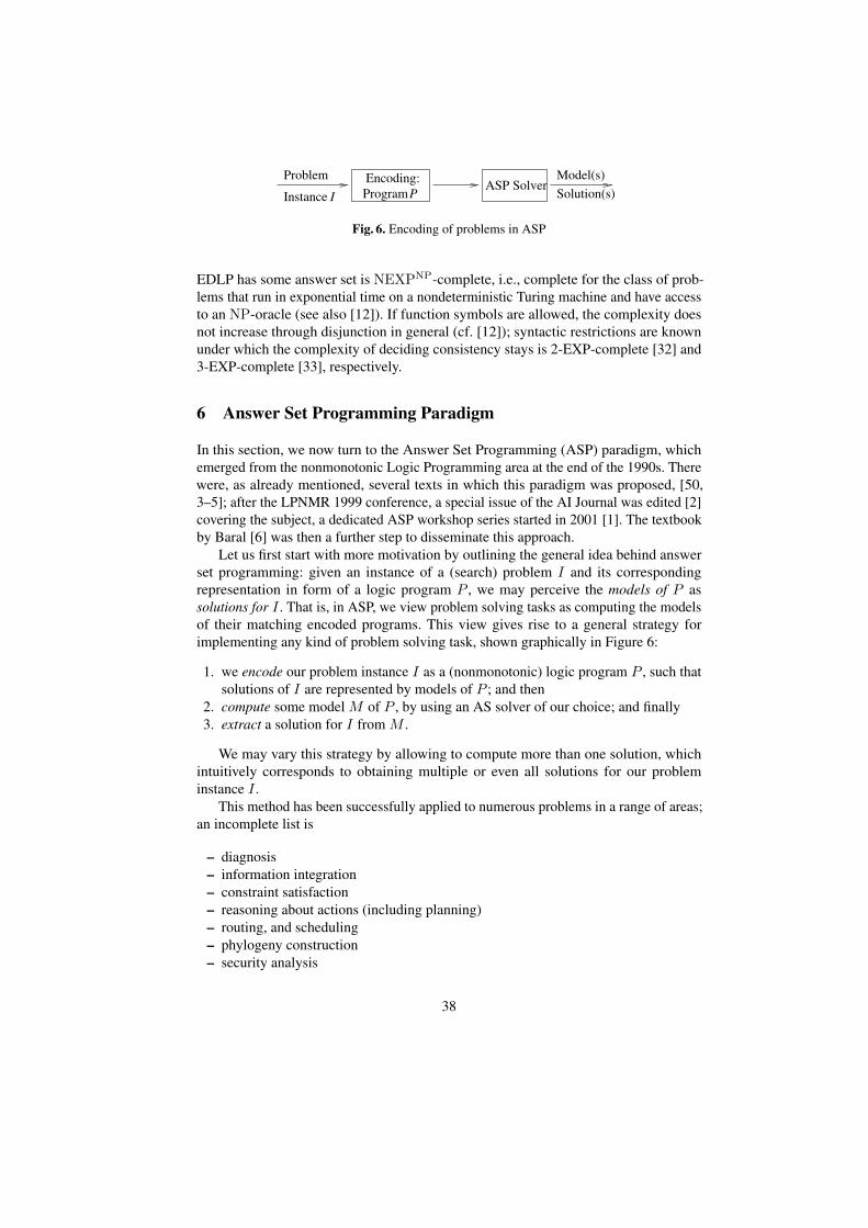
Problem

Instance I ProgramP

Encoding: Model(s)

Solution(s)ASP Solver

Fig. 6. Encoding of problems in ASP

EDLP has some answer set is NEXPNP-complete, i.e., complete for the class of prob-lems that run in exponential time on a nondeterministic Turing machine and have accessto an NP-oracle (see also [12]). If function symbols are allowed, the complexity doesnot increase through disjunction in general (cf. [12]); syntactic restrictions are knownunder which the complexity of deciding consistency stays is 2-EXP-complete [32] and3-EXP-complete [33], respectively.

6 Answer Set Programming Paradigm

In this section, we now turn to the Answer Set Programming (ASP) paradigm, whichemerged from the nonmonotonic Logic Programming area at the end of the 1990s. Therewere, as already mentioned, several texts in which this paradigm was proposed, [50,3–5]; after the LPNMR 1999 conference, a special issue of the AI Journal was edited [2]covering the subject, a dedicated ASP workshop series started in 2001 [1]. The textbookby Baral [6] was then a further step to disseminate this approach.

Let us first start with more motivation by outlining the general idea behind answerset programming: given an instance of a (search) problem I and its correspondingrepresentation in form of a logic program P , we may perceive the models of P assolutions for I . That is, in ASP, we view problem solving tasks as computing the modelsof their matching encoded programs. This view gives rise to a general strategy forimplementing any kind of problem solving task, shown graphically in Figure 6:

1. we encode our problem instance I as a (nonmonotonic) logic program P , such thatsolutions of I are represented by models of P ; and then

2. compute some model M of P , by using an AS solver of our choice; and finally3. extract a solution for I from M .

We may vary this strategy by allowing to compute more than one solution, whichintuitively corresponds to obtaining multiple or even all solutions for our probleminstance I .

This method has been successfully applied to numerous problems in a range of areas;an incomplete list is

– diagnosis– information integration– constraint satisfaction– reasoning about actions (including planning)– routing, and scheduling– phylogeny construction– security analysis

38

– configuration– computer-aided verification– health care– biomedicine and biology– Semantic Web– knowledge management– text mining and classification– question answering

The survey [51] is a source for specific applications, some of which can be viewedin an online showcase collection.16

We illustrate the ASP approach on the problem of computing legal 3-colorings of agraph.

Example 32. Let G = (V,E) be a graph with nodes V = {a, b, c, d} and edges E ={(a, b), (b, c), (c, a), (a, d)}, which constitutes our problem instance I . We can encodethe legal three colorings of G into answer sets of a logic program P as follows. For eachnode n, we have atoms bn, rn, and gn which informally mean that node n is coloredblue, red, and green, respectively. Then we set up the following rules. For each noden ∈ V ,

bn ← not rn,not gn.rn ← not bn,not gn.gn ← not rn,not bn.

and for each edge (n, n′) in E, the constraints

← bn, bn′ .← rn, rn′ .← gn, gn′ .

Then, the answer sets of P encode 1-1 the legal 3-colorings of G. Informally, the rulesfor n ∈ V assign one of the three colors to n, and the constraints for (n, n′) check thatadjacent nodes do not have the same color. Equally well, we can replace the three rulesfor n ∈ V by the single (and perhaps more intuitive) rule

bn ∨ rn ∨ gn ← .

This problem solving strategy is closely related to similar approaches like SAT-solving, where the problem instance is encoded onto the (classical) models of a propo-sitional formula of clause set. It is because of this that some authors refer to AnswerSet Programming as the more general paradigm in which a problem is encoded into themodels of a logical theory, and consider the usage of nonmonotonic logic programs astheory as a particular instance of this paradigm. We prefer here, however, to reservethe term ASP for the setting with nonmonotonic logic programs under the answer setsemantics itself.16 http://www.kr.tuwien.ac.at/research/projects/WASP/showcase.html

39

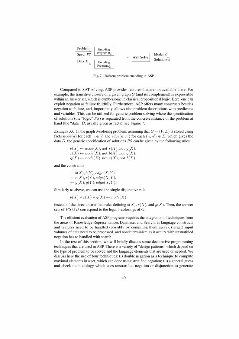
Program PPS

Encoding:

Program PD

Encoding:

ASP SolverModel(s)

Solution(s)

PSSpec.

Problem

DData

Fig. 7. Uniform problem encoding in ASP

Compared to SAT solving, ASP provides features that are not available there. Forexample, the transitive closure of a given graph G (and its complement) is expressiblewithin an answer set, which is cumbersome in classical propositional logic. Here, one canexploit negation as failure fruitfully. Furthermore, ASP offers many constructs besidesnegation as failure, and, importantly, allows also problem descriptions with predicatesand variables. This can be utilized for generic problem solving where the specificationof solutions (the “logic” PS ) is separated from the concrete instance of the problem athand (the “data” D, usually given as facts); see Figure 7.

Example 33. In the graph 3-coloring problem, assuming that G = (V,E) is stored usingfacts node(n) for each n ∈ V and edge(n, n′) for each (n, n′) ∈ E, which gives thedata D, the generic specification of solutions PS can be given by the following rules:

b(X)← node(X),not r(X),not g(X).r(X)← node(X),not b(X),not g(X).g(X)← node(X),not r(X),not b(X).

and the constraints

← b(X), b(Y ), edge(X,Y ).← r(X), r(Y ), edge(X,Y ).← g(X), g(Y ), edge(X,Y ).

Similarly as above, we can use the single disjunctive rule

b(X) ∨ r(X) ∨ g(X)← node(X).

instead of the three unstratified rules defining b(X), r(X), and g(X). Then, the answersets of PS ∪D correspond to the legal 3-colorings of G.

The efficient evaluation of ASP programs requires the integration of techniques fromthe areas of Knowledge Representation, Database, and Search, as language constructsand features need to be handled (possibly by compiling them away), (larger) inputvolumes of data need to be processed, and nondeterminism as it occurs with unstratifiednegation has to handled with search.

In the rest of this section, we will briefly discuss some declarative programmingtechniques that are used in ASP. There is a variety of “design patterns” which depend onthe type of problem to be solved and the language elements that are used or needed. Wediscuss here the use of four techniques: (i) double negation as a technique to computemaximal elements in a set, which can done using stratified negation; (ii) a general guessand check methodology which uses unstratified negation or disjunction to generate

40

and prune solutions candidates; (iii) an advanced technique called saturation, whichcan be used in disjunctive logic programming to test properties of various subsets of aset within an answer set, and is essential to solve “hard” problems there (cf. [48, 52]);(iv) in combination with this, iteration over a set to test whether a property holds for allelements without the use of negation.

6.1 Use of Double Negation

The first technique which we look at is the use of double negation. In classical logic¬¬A ≡ A, i.e., double negation can be canceled. This can be similarly exploited inASP to define a predicate p(X) in terms of its complement −p(x), and is particularlyattractive if −p(x) can be defined easily. For example, one can avoid counting andarithmetic for determining the maximum in a (finite) set of numbers.

Example 34. Suppose the data about employees of a company and their salaries arestored as facts empl(N,S) in the data D, where N is the name and S the salary of anemployee. Then the maximum salary, s∗ = max{s | empl(e, s) ∈ D}, is determinedby the following simple ASP program:

% salary S is *not* maximal−max(S)← empl(N,S), empl(N1, S1), S < S1.

% double negationmax(S)← empl(N,S),not −max(S).

Example 35. For a little more involved example where this technique can be usedsuccessfully, consider the problem of computing the greatest common divisor (gcd) oftwo natural numbers n,m > 0; recall that the gcd of n and m is the largest integerd∗ such that d∗ divides both n and m. This problem is a standard example in logicprogramming and elegant solutions for it can be found in textbooks, which basicallyimplement Euclid’s recursive algorithm for it by rules:

% base casegcd(X,X,X)← int(X), X > 1.% subtract smaller from larger numbergcd(D,X, Y )← X < Y, gcd(D,X, Y1), Y = Y1 +X.gcd(D,X, Y )← X > Y, gcd(D,X1, Y ), X = X1 + Y.

Here, int(X) is a (built in) predicate for natural numbers ≥ 0. While Euclid’s algorithmis ingenious, the average programmer will approach the problem by trying to cast thedefinition into rules. Here, double negation can be used again to single out the maximalcommon divisor d∗ in the predicate gcd(X,Y, Z) given that the common divisors arecomputed in a predicate cd(X,Y, Z), which in turn can be done easily using a predicatedivisor(X,Y ) that is defined using simple (built-in) arithmetic. A respective programis the following:

% Declare when D divides a number N .divisor(D,N)← int(D), int(N), int(M), N = D ∗M.% Declare common divisors

41

cd(T,N1, N2)← divisor(T,N1), divisor(T,N2).% Single out non-maximal common divisors T−gcd(T,N1, N2)← cd(T,N1, N2), cd(T1, N1, N2), T < T1.% Apply double negation: take non non-maximal divisorgcd(T,N1, N2)← cd(T,N1, N2), not − gcd(T,N1, N2).

For a similar encoding in Prolog, one has to be careful to define and use int(X) properlyin the rules, otherwise the program might not terminate.

Note that the above programs are both stratified and thus have a single answerset over any input data (provided that some answer set exists). We will next considerprograms that are geared toward multiple answer sets for capturing problems withmultiple solutions.

6.2 The “Guess and Check” Methodology

An important element of ASP is to employ a “Guess and Check” methodology, which issometimes also called Generate-and-Test [3]. The idea is here to proceed as follows:

1. use nondeterminism that comes with unstratified negation, or equally well withdisjunction in rule heads, to create candidate solutions to a problem (program partG), and

2. to check with further rules and/or constraints, whether a solution candidate is proper(program part C). This part may also involve auxiliary predicates, if needed.

From another perspective, the part G defines the search space, and the part C prunesillegal branches. A detailed discussion of this paradigm is given in [53, 52], and in [53] itis extended by a further component to compute optimal solutions (we will deal with thisin Section 7.2 below). We will just briefly illustrate the methodology on a few examples.

Example 36. As a first example, we revisit the 3-colorability problem in Example 33.

g(X) ∨ r(X) ∨ b(X)← node(X)}

Guess

← b(X), b(Y ), edge(X,Y )← r(X), r(Y ), edge(X,Y )← g(X), g(Y ), edge(X,Y )

Check

The first disjunctive rule constitutes the guessing part G, which generates all possibleassignments of one colors to the nodes of the graph, while the three constraints constitutethe checking part C.

The next example shows a checking part which uses auxiliary predicates.

Example 37. Recall that for a directed graph G = (V,E), a path n0 → n1 → · · · → nkin G from a start node n0 ∈ V is called a Hamiltonian path, if all nodes ni are distinctand each node in V occurs in the path, i.e., V = {n0, . . . , nk}. Assume that, as above,the graphG is stored using the predicates node(X) and edge(X,Y ), and that a predicatestart(X) stores the unique node n0. Consider the following program:

42

inPath(X,Y ) ∨ outPath(X,Y ) ← edge(X,Y ).}

Guess

← inPath(X,Y ), inPath(X,Y1), Y 6= Y1.← inPath(X,Y ), inPath(X1, Y ), X 6= X1.← node(X), not reached(X).

Check

reached(X)← start(X).reached(X)← reached(Y ), inPath(Y,X).

}Auxiliary Predicate

The guessing part G simple states for each edge of the graph whether it belongs to thepath or not. The checking part C tests whether inPath really constitutes a path in Gin which each node occurs only once (which is ensured if there is at most one edgefrom/to each node), and that all nodes are on the path. For this, the auxiliary predicatereached(X) is used, which expresses that the node X is reached from the starting node.The latter is expressed with two simple recursive rules.

Note that deciding the existence of a Hamiltonian path is, like 3-colorability, NP-complete; a similar SAT encoding would be, due to the reachability check, more cumber-some.

As a final example, we consider a scenario where the checking part is interfering withthe guessing part, which shows that the two parts may not always be cleanly separated.In fact, this happens for the elementary task of choosing an element from a set.

Example 38. Suppose departments of a company are stored in a predicate dept(X), andthe task is to choose a single department; in general, there will be multiple choices (ornone, if dept would be empty). The following program is a simple (yet little elegant)solution to the problem:

sel(D)∨ −sel(D)← dept(D)}

Guess

← sel(D1), sel(D2), D1 6= D2

some sel← sel(D)← dept(D),not some sel

Check

Here, the checking part tests that not more than one department has been chosen, andthat at least one is chosen if there are departments (hence, exactly one is chosen).

A more elegant solution is to let the checking part interfere with the guessing part,and to exploit the minimality property of answer sets.

sel(D)← dept(D),not −sel(D)}

Guess−sel(D1)← dept(D1), sel(D2), D1 6= D2

}Check

The guessing rules informally states that, by default, a department D is chosen. Thechecking rule says that if some department is chosen, then all others can not be chosen;this is fed back to the guessing part. In combination, since not all departments have to beexcluded from selection, exactly one will be chosen in an answer set (provided somedepartments exist, otherwise ∅ is the single answer set). In other words, the only stableconfigurations of the above program are those in which one and only one atom of typesel(v) is present.

Note that we could equally well replace the checking rule with the rule

43

−sel(D1) ∨ −sel(D2)← dept(D1), dept(D2), D1 6= D2.

Informally, this rule says that if we have two different departments, then at least one ofthem can not be selected.

As a final example for choice, we consider a simple course scheduling scenario.

Example 39. Suppose there is a computer science department cs at a university u. Wehave information about members and courses of cs , as well as preferred courses ofmembers, both encoded as facts F :

member(sam, cs). course(java, cs). course(ai , cs).

member(bob, cs). course(c, cs). course(logic, cs).

member(tom, cs).

likes(sam, java). likes(sam, c).

likes(bob, java). likes(bob, ai).

likes(tom, ai). likes(tom, logic).

Our task is now to assign each member of the department some courses, such that(i) each member should have at least one course, (ii) nobody should have more thantwo courses, and (iii) assign only courses that the course leader likes. We can use thefollowing program P to encode this problem:

teaches(X,Y )← member(X, cs), course(Y, cs), likes(X,Y ),

not−teaches(X,Y ).

−teaches(X,Y )← member(X, cs), course(Y, cs), teaches(X1, Y ), X1 6= X.

some course(X)← member(X, cs), teaches(X,Y ).

← member(X, cs),not some course(X).

← teaches(X,Y1), teaches(X,Y2), teaches(X,Y3),

Y1 6= Y2, Y1 6= Y3, Y2 6= Y3.

Informally, the first rule says that a CS faculty member gets a CS course she likesassigned by default. The second rule states that a CS faculty member does not get a CScourse assigned if somebody else teaches it. The third and fourth rules make sure thateach CS faculty gets at least one course assigned. The final rule excludes any assignmentwhere one person is assigned three (or more) courses.

We obtain the following three answer sets of P ∪ F :

– {teaches(sam, c), teaches(bob, java), teaches(bob, ai), teaches(tom, logic), . . .}– {teaches(sam, java), teaches(sam, c), teaches(bob, ai), teaches(tom, logic), . . .}– {teaches(sam, c), teaches(bob, java), teaches(tom, ai), teaches(tom, logic), . . .}

6.3 Saturation Technique

A more advanced technique that is used in disjunctive ASP is the so called saturationtechnique, which is used to check whether all possible guesses satisfy a certain property,

44

like not being a solution to a problem. Testing such a property, like whether all assign-ments of three colors to nodes do not legally color a graph G, may be co-NP-hard, andthus can not be evidently encoded in a normal logic program such that the program hassome answer set precisely if G is not 3-colorable; in fact, the program in Example 33has no answer set if G is not 3-colorable.

It is, however, possible to express the property of non-3-colorability by a uniqueanswer set candidate for a program, such that the candidate is the only answer set if thegraph is not 3-colorable, and is not an answer set otherwise. More abstractly, to test aproperty we design a program P and an answer set candidate Msat such that Msat isthe single answer set of P if the property holds, and P has other answer sets (excludingMsat ) otherwise. The construction is such that any answer set of P is a subset of Msat ,and whenever the property is found to hold, any candidate answer set is “saturated” toMsat . Intuitively, the property is tested within the answer set.

Example 40. For testing non-3-colorability, the constraints in the checking part of theprogram in Example 33 can be replaced, thus obtaining the program Pnon col:

b(X) ∨ r(X) ∨ g(X)← node(X).non col ← r(X), r(Y ), edge(X,Y ).non col ← g(X), g(Y ), edge(X,Y ).non col ← b(X), b(Y ), edge(X,Y ).χ(X)← non col , node(X).

where χ ∈ {r, g, b}. Informally, this change has the following effect: Whenever anassignment of colors to the nodes is bad, the assignment is rejected by “saturating” thecandidate model at hand, selecting all ground facts r(n), g(n), and b(n) for any node n.Importantly, the saturation is the same for all bad assignments. Thus, if all assignmentsof colors are bad, there will a be single answer set Msat of the program, which contains,besides the graph description, non col and r(n), g(n), and b(n) for any node n. Onthe other hand, any good assignment of colors will lead to an answer set M such thatM ⊂ Msat , which means that Msat is not an answer set of the program, and thatPnon col has many answer sets, smaller than Msat corresponding to valid 3-colorings.Thus, Msat is the single answer set of the program just if the graph is not 3-colorable.Note also that Pnon col |=c non col iff the graph at hand is not 3-colorable.

We can abstract from the previous example a general design rule: if we desire tocheck that a property Pr holds for all guesses defining a search space, we can establisha guess and saturation check paradigm as follows:

– Define the search space of guesses through a subprogram Pguess , using disjunctiverules.

– Define a subprogram Pcheck , which checks Pr for a guess Mg .– If Pr holds for Mg , an appropriate set of saturation rules Psat generates the special

candidate answer set Msat.– If Pr does not hold for Mg, an answer set results which is a strict subset of Msat

(thus preventing that Msat is an answer set).

It is thus crucial that the program Pcheck , which formalizes Pr , and Psat do notgenerate incomparable candidate answer sets. Incomparability might be easily introduced,

45

besides subprograms with negation as failure, by improper use of disjunction, or byill-designed (positive) saturation rules; we will see an example in the next subsection.

In combination with further guessing rules, which assign values to atoms that are notinvolved in saturation, it is possible to express problems that have complexity beyondNP, like the strategic companies problem [53, 52], or quantified Boolean formulas ofthe form ∃X∀Y E(X,Y ), which are Σp

2 -complete.

6.4 Iteration over a Set

As last technique, we consider testing a property for all elements of a set without the useof negation. This may be needed in some contexts, for instance in combination with thesaturation technique, or when the use of negation could lead to undesired behavior (e.g.,in case of cyclic negation).

Example 41. Suppose we want to test whether in a directed graph G = (V,E), all nodesare reachable from a designated start node n0 ∈ V . Using the representation of G andn0 as in Example 37, we could use the following rules and double negation:

all reached← not −all reached.−all reached← node(X),not reached(X).reached(X)← start(X).reached(X)← reached(Y ), edge(Y,X).

Here, all reached is true in the resulting answer set, exactly if all nodes are reachablefrom n0.

Now suppose that we want to test in an answer set whether reachability holds foreach graph G′ that results from G by removing between all nodes n and n′, that aremutually connected, one of the edges n→ n′, n′ → n at random. The edges of G′ canbe generated using the rules

edge1(X,Y ) ∨ edge1(Y,X)← edge(X,Y ), edge(Y,X).edge1(X,Y )← edge(X,Y ),not edge(Y,X).

Let us replace edge in the rules for reached with edge1 and add the saturation rule

edge1(X,Y )← all reached, edge(X,Y ).

We thus obtain the program Pg:

all reached← not −all reached.−all reached← node(X),not reached(X).reached(X)← start(X).reached(X)← reached(Y ), edge(Y,X).edge1(X,Y ) ∨ edge1(Y,X)← edge(X,Y ), edge(Y,X).edge1(X,Y )← edge(X,Y ),not edge(Y,X).edge1(X,Y )← all reached, edge(X,Y ).

However Pg does not work as expected, as evidenced, e.g., by the simple graphG = ({a, b}, {a→ b, b→ a}), where for n0 = a we get that the candidate

46

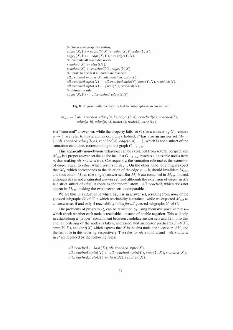
% Guess a subgraph for testingedge1(X,Y ) ∨ edge1(Y,X)← edge(X,Y ), edge(Y,X).edge1(X,Y )← edge(X,Y ), not edge(Y,X).% Compute all reachable nodesreached(X)← start(X).reached(X)← reached(Y ), edge1(Y,X).% iterate to check if all nodes are reachedall reached← last(X), all reached upto(X).all reached upto(X)← all reached upto(Y ), succ(Y,X), reached(X).all reached upto(X)← first(X), reached(X).% Saturation ruleedge1(X,Y )← all reached, edge(X,Y ).

Fig. 8. Program with reachability test for subgraphs in an answer set

Msat = { all reached, edge1(a, b), edge1(b, a), reached(a), reached(b),edge(a, b), edge(b, a), node(a), node(b), start(a)}

is a “saturated” answer set, while the property fails for G (for a witnessing G′, removea → b; we refer to this graph as G−(a→b)). Indeed, P has also an answer set M2 ={−all reached, edge1(b, a), reached(a), edge(a, b), . . .}, which is not a subset of thesaturation candidate, corresponding to the graph G−(a→b).

This apparently non-obvious behaviour can be explained from several perspectives:Msat is a proper answer set due to the fact that G−(b→a) reaches all possible nodes froma, thus making all reached true. Consequently, the saturation rule makes the extensionof edge1 equal to edge, which results in Msat. On the other hand, one might expectthat M2, which corresponds to the deletion of the edge a→ b, should invalidate Msat,and thus obtain M2 as (the single) answer set. But M2 is not contained in Msat. Indeed,although M2 is not a saturated answer set, and although the extension of edge1 in M2

is a strict subset of edge, it contains the “spare” atom −all reached, which does notappear in Msat, making the two answer sets incomparable.

We are thus in a situation in which Msat is an answer set, resulting from some of theguessed subgraphs G′ of G in which reachability is retained, while we expected Msat asan answer set if and only if reachability holds for all guessed subgraphs G′ of G.

The problems of program Pg can be remedied by using recursive positive rules—which check whether each node is reachable—instead of double negation. This will helpin establishing a “proper” containment between candidate answer sets and Msat. To thisend, an ordering of the nodes is taken, and associated successor predicates first(X),succ(Y,X), and last(X) which express that X is the first node, the successor of Y , andthe last node in this ordering, respectively. The rules for all reached and −all reachedin P are replaced by the following rules:

all reached← last(X), all reached upto(X).all reached upto(X)← all reached upto(Y ), succ(Y,X), reached(X).all reached upto(X)← first(X), reached(X).

47

if we add then the respective facts for the ordering, the resulting program (see Fig-ure 8) works as desired. Informally, these rules access the (positive) reachability that iscomputed by the rules for reached with respect to varying subgraphs G′ of G.

The use of an ordering and a rule scheme as above can be easily applied in othercontexts. In case the set over which the iteration is made is susceptible to change itself(e.g., if in the previous example only all nodes that have no outgoing edges need to bereached), then special rules can be added that skip elements, indicated by out(X):

all reached upto(X)← all reached upto(Y ), succ(Y,X), out(X).all reached upto(X)← first(X), out(X).

where out is computed using positive rules; the formulation for the continued exampleis left as a (simple) exercise.

7 Answer Set Solvers

In this section, we mention some AS solvers and briefly present the DLV system.Given that deciding whether a given extended logic program has some answer set is

NP-complete, it is clear that efficient computation of answer sets is not easy, and that wecan not expect to have a polynomial time algorithm for this task (even under polynomialtotal-time, i.e., if the combined size of the input P and the output in terms of all answersets of P is measured). In fact, the problem is yet harder if disjunction in rule heads isallowed.

A number of different, sophisticated algorithms have been developed over the past15 years (similar as in the area of SAT solving), and to date a number of AS solvers areavailable; a partial list is shown in Table 1. Some of these solvers provide a number ofextensions to the language described here, and have been further developed into familiesof solvers (e.g. the DLV system).

A collection of benchmark problems for AS solvers is maintained at the ASPARA-GUS platform,17 where also information about language formats and the ASP SystemCompetition (whose first edition was at the LPNMR 2007 conference) can be found.In the next subsection, we briefly address implementation strategies of AS solvers; anexcellent source on this topic is Ilkka Niemela’s ICLP’04 tutorial.18

7.1 Architecture of ASP Solvers

Traditional answer set solvers typically have a two level architecture:

1. Grounding Step: Given a program P with variables, a (subset) P ′ of its groundingis generated which has the same answer sets as P .

2. Model Search: The answer sets of the grounded (propositional) program P ′ arecomputed.

17 http://asparagus.cs.uni-potsdam.de/18 http://www.tcs.hut.fi/˜ini/papers/niemela-iclp04-tutorial.ps.gz.

48

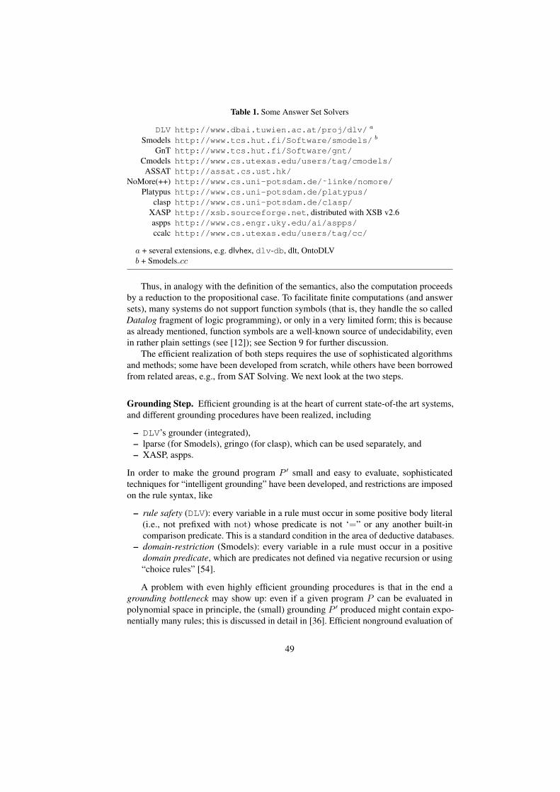
Table 1. Some Answer Set Solvers

DLV http://www.dbai.tuwien.ac.at/proj/dlv/ a

Smodels http://www.tcs.hut.fi/Software/smodels/ b

GnT http://www.tcs.hut.fi/Software/gnt/Cmodels http://www.cs.utexas.edu/users/tag/cmodels/

ASSAT http://assat.cs.ust.hk/NoMore(++) http://www.cs.uni-potsdam.de/˜linke/nomore/

Platypus http://www.cs.uni-potsdam.de/platypus/clasp http://www.cs.uni-potsdam.de/clasp/

XASP http://xsb.sourceforge.net, distributed with XSB v2.6aspps http://www.cs.engr.uky.edu/ai/aspps/ccalc http://www.cs.utexas.edu/users/tag/cc/

a + several extensions, e.g. dlvhex, dlv-db, dlt, OntoDLVb + Smodels cc

Thus, in analogy with the definition of the semantics, also the computation proceedsby a reduction to the propositional case. To facilitate finite computations (and answersets), many systems do not support function symbols (that is, they handle the so calledDatalog fragment of logic programming), or only in a very limited form; this is becauseas already mentioned, function symbols are a well-known source of undecidability, evenin rather plain settings (see [12]); see Section 9 for further discussion.

The efficient realization of both steps requires the use of sophisticated algorithmsand methods; some have been developed from scratch, while others have been borrowedfrom related areas, e.g., from SAT Solving. We next look at the two steps.

Grounding Step. Efficient grounding is at the heart of current state-of-the art systems,and different grounding procedures have been realized, including

– DLV’s grounder (integrated),– lparse (for Smodels), gringo (for clasp), which can be used separately, and– XASP, aspps.

In order to make the ground program P ′ small and easy to evaluate, sophisticatedtechniques for “intelligent grounding” have been developed, and restrictions are imposedon the rule syntax, like

– rule safety (DLV): every variable in a rule must occur in some positive body literal(i.e., not prefixed with not) whose predicate is not ‘=” or any another built-incomparison predicate. This is a standard condition in the area of deductive databases.

– domain-restriction (Smodels): every variable in a rule must occur in a positivedomain predicate, which are predicates not defined via negative recursion or using“choice rules” [54].

A problem with even highly efficient grounding procedures is that in the end agrounding bottleneck may show up: even if a given program P can be evaluated inpolynomial space in principle, the (small) grounding P ′ produced might contain expo-nentially many rules; this is discussed in detail in [36]. Efficient nonground evaluation of

49

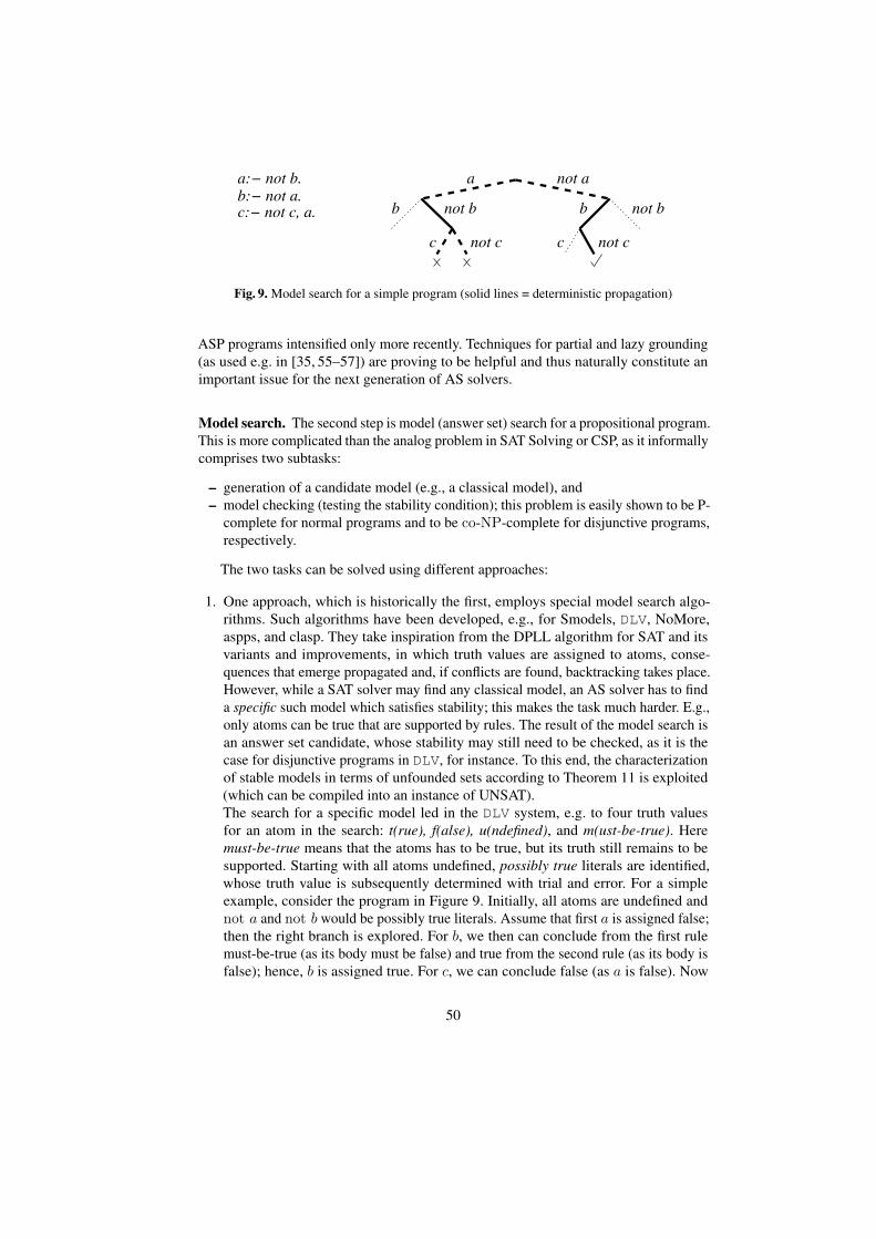
b:− not a.

a:− not b.

c:− not c, a.

not aa

c not c

not bbnot b

c not c

b

Fig. 9. Model search for a simple program (solid lines = deterministic propagation)

ASP programs intensified only more recently. Techniques for partial and lazy grounding(as used e.g. in [35, 55–57]) are proving to be helpful and thus naturally constitute animportant issue for the next generation of AS solvers.

Model search. The second step is model (answer set) search for a propositional program.This is more complicated than the analog problem in SAT Solving or CSP, as it informallycomprises two subtasks:

– generation of a candidate model (e.g., a classical model), and– model checking (testing the stability condition); this problem is easily shown to be P-

complete for normal programs and to be co-NP-complete for disjunctive programs,respectively.

The two tasks can be solved using different approaches:

1. One approach, which is historically the first, employs special model search algo-rithms. Such algorithms have been developed, e.g., for Smodels, DLV, NoMore,aspps, and clasp. They take inspiration from the DPLL algorithm for SAT and itsvariants and improvements, in which truth values are assigned to atoms, conse-quences that emerge propagated and, if conflicts are found, backtracking takes place.However, while a SAT solver may find any classical model, an AS solver has to finda specific such model which satisfies stability; this makes the task much harder. E.g.,only atoms can be true that are supported by rules. The result of the model search isan answer set candidate, whose stability may still need to be checked, as it is thecase for disjunctive programs in DLV, for instance. To this end, the characterizationof stable models in terms of unfounded sets according to Theorem 11 is exploited(which can be compiled into an instance of UNSAT).The search for a specific model led in the DLV system, e.g. to four truth valuesfor an atom in the search: t(rue), f(alse), u(ndefined), and m(ust-be-true). Heremust-be-true means that the atoms has to be true, but its truth still remains to besupported. Starting with all atoms undefined, possibly true literals are identified,whose truth value is subsequently determined with trial and error. For a simpleexample, consider the program in Figure 9. Initially, all atoms are undefined andnot a and not b would be possibly true literals. Assume that first a is assigned false;then the right branch is explored. For b, we then can conclude from the first rulemust-be-true (as its body must be false) and true from the second rule (as its body isfalse); hence, b is assigned true. For c, we can conclude false (as a is false). Now

50

all atoms are either true or false; the candidate M = {b} is indeed an answer setand output. Coming back to the root, a is alternatively assigned must-be-true. Fromthe first rule, we would then conclude that b is false, which in turn makes a true;further, one would conclude that not c is possibly true. However, setting c to falseleads to a conflict (by the third rule c then would have to be true), and also setting cto must-be-true, as then c has no support and must be false.Important for these approaches are heuristics (which atom/rule to consider next); formore details concerning DLV, see [58, 59].

2. Later, another approach was to translate the logic program to SAT Solving, whichhas been realized e.g. in ASSAT and Cmodels. To this end, as already mentioned inSection 5.3 the so called Clark completion of a logic program [46] (which translatesan acyclic program into an equivalent SAT instance) is extended with loop formulas[43, 44].Note that for SAT, model checking is easy in terms of complexity, and can be donein LOGSPACE (in fact, the problem is solvable in ALOGTIME, which is far downin LOGSPACE).19 An attractive advantage of this approach is that it can benefitfrom improvements to SAT solving technology; drawbacks are that to generate allanswer sets, one needs a SAT solver that can compute all models of a clause set (orone has to tune the transformation for incremental enumeration of answer sets) andthat in general, the SAT instance that is constructed can have exponential size.

7.2 The DLV System

As an example of an AS solver, we briefly consider here the DLV system. 20 DLV is astate-of-the-art answer set solver which has been developed at the Vienna University ofTechnology and the University of Calabria over more than a decade, starting out with aresearch project on non-monotonic deductive databases in 1996; it is freely available fordownload.

The system has a language that is richer than the extended disjunctive logic programsconsidered above, and supports additional constructs (e.g., aggregates, weak constraints)some of which increase the expressivity (e.g., weak constraints allow to express optimiza-tion problems with complexity beyond Σp

2 ). DLV supports certain built-in predicates(e.g. bounded integer arithmetic and comparisons), and offers a range of front-ends forspecific KR tasks (e.g., planning or diagnosis), as well an interface to databases. Theprinciple reasoning tasks supported by DLV are 1. answer set generation (all or a givennumber) and 2. brave and cautious query answering, which is supported for both groundand non-ground queries.

The DLV system has been described in many publications, of which [53] is the mostcomprehensive; the article [60] is recent. As mentioned above, its reasoning engineimplements the two-level architecture outlined in Section 7, using a highly optimizedgrounding module for the first level; the model search is by a DPLL style algorithm

19 This also intuitively is a clue why there are so many loop formulas, made more precise in [47]:if there were few and they could be easily constructed, we could solve a P-complete (resp.co-NP-complete) problem in LOGSPACE (resp., in polynomial time).

20 http://www.dbai.tuwien.ac.at/proj/dlv/

51

that uses the characterization of stable models by unfounded sets in Theorem 11. DLValso incorporates a lot of deductive database technology in order to handle larger datavolumes (including magic sets, which have been generalized to programs with negationand disjunction). The DLV engine has been extended in many directions leading to afamily of systems that support different purposes, including dlv-ex, dlvhex, OntoDLV,dlv-db, and dlt.

DLV syntax. Briefly, the core language of DLV consists of rules of the form

a1 v · · · v an :- b1, · · · , bk, not bk+1, · · · , not bm.

where n + m > 1, and all ai, bj are atoms or strongly negated atoms (e.g. −a); nofunction symbols are allowed; the syntax of terms is like in Prolog. Certain built-inpredicates are supported (cf. Table 2). Note that DLV allows constraints (n = 0); asmentioned in Section 7.1, DLV requires rule safety. The extended language also allowsthat the bj are aggregate atoms, in which the values of aggregate functions over aconjunction of literals (including # max, # min, #sum, #count, and #times), canbe compared to given bounds; we refer to [61] for details.

Furthermore, the DLV language has weak constraints, which are of the form

:∼ b1, · · · , bk, not bk+1, · · · , not bm. [w : l] (28)

where all bj are as in rules and w (the weight) and l (the level, or layer) are positiveinteger constants or variables. For convenience, w and/or l can be omitted and are set to1 in this case. Informally, the expression (28) is a constraint that can be violated, whichincurs cost w; for an answer set, the costs of all violated (instances of) weak constraintsare added up, grouped by levels of priorities l. Among all answer sets, those whosecost vector is lexicographically (ordered by priority) smallest are chosen as optimalanswer sets; see [53] for formal details. With the help of weak constraints, the Guessand Check methodology in Section 6.2 can be extended to a Guess, Check and OptimizeMethodology (an example follows shortly).

Queries are specified in DLV by expressions

b1, · · · , bk, not bk+1, · · · , not bm?

where all bj are atoms or strongly negated atoms; the query mode (brave or cautious) isselected using a switch (–brave resp. –cautious). Variables in queries are allowed; allbindings of variables to constants will be shown such that the resulting ground queryevaluates to true; if the query is ground, in case of brave reasoning a witnessing answerset is shown.21

Example 42. To illustrate the use of weak constraints, we consider the well-knownTraveling Salesperson problem (TSP), where cities are stored as facts city(X) and directconnections as facts conn(X,Y,C), where C is the cost of traveling from X to Y .Furthermore, the tour is required to start in a city designated with a fact start(X).

The following DLV program computes optimal tours in its optimal answer sets:21 Unless magic sets are enabled, which will be the default in future DLV releases.

52

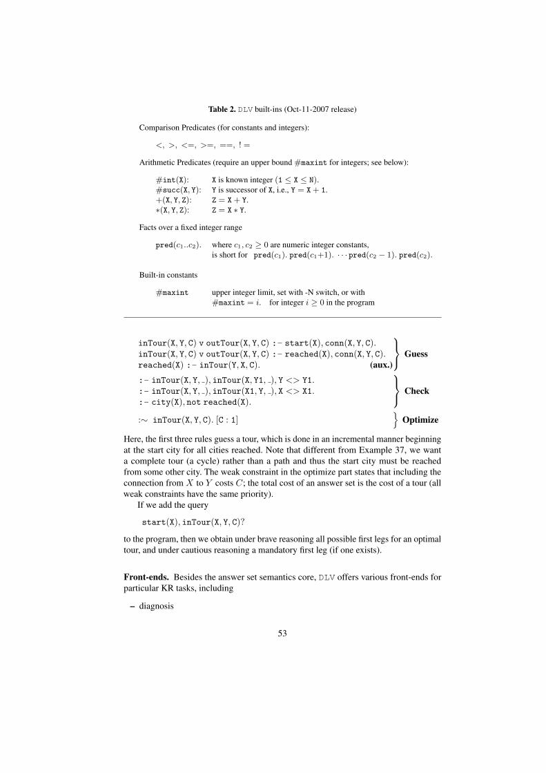
Table 2. DLV built-ins (Oct-11-2007 release)

Comparison Predicates (for constants and integers):

<, >, <=, >=, ==, ! =

Arithmetic Predicates (require an upper bound #maxint for integers; see below):

#int(X): X is known integer (1 ≤ X ≤ N).#succ(X, Y): Y is successor of X, i.e., Y = X+ 1.+(X, Y, Z): Z = X+ Y.∗(X, Y, Z): Z = X ∗ Y.

Facts over a fixed integer range

pred(c1..c2). where c1, c2 ≥ 0 are numeric integer constants,is short for pred(c1). pred(c1+1). · · · pred(c2 − 1). pred(c2).

Built-in constants

#maxint upper integer limit, set with -N switch, or with#maxint = i. for integer i ≥ 0 in the program

inTour(X, Y, C) v outTour(X, Y, C) :- start(X), conn(X, Y, C).inTour(X, Y, C) v outTour(X, Y, C) :- reached(X), conn(X, Y, C).reached(X) :- inTour(Y, X, C). (aux.)

Guess

:- inTour(X, Y, ), inTour(X, Y1, ), Y <> Y1.:- inTour(X, Y, ), inTour(X1, Y, ), X <> X1.:- city(X), not reached(X).

Check

:∼ inTour(X, Y, C). [C : 1]}

Optimize

Here, the first three rules guess a tour, which is done in an incremental manner beginningat the start city for all cities reached. Note that different from Example 37, we wanta complete tour (a cycle) rather than a path and thus the start city must be reachedfrom some other city. The weak constraint in the optimize part states that including theconnection from X to Y costs C; the total cost of an answer set is the cost of a tour (allweak constraints have the same priority).

If we add the query

start(X), inTour(X, Y, C)?

to the program, then we obtain under brave reasoning all possible first legs for an optimaltour, and under cautious reasoning a mandatory first leg (if one exists).

Front-ends. Besides the answer set semantics core, DLV offers various front-ends forparticular KR tasks, including

– diagnosis

53

– knowledge-based planning (K language)– front-end to SQL3– inheritance reasoning

The first three front-ends can be invoked using command-line switches, while theinheritance front-end is automatically enabled if the input is an inheritance program [62].Many other front-ends, created by various authors, are available as separate packages.

Using DLV. The DLV system is primarily command-line oriented, but there is also aplain GUI and there are web interfaces available.22

The system reads input from files whose names are passed on the command-line. Ifthe command-line option “--” has been specified, input is also read from standard input(stdin). Output is printed to standard output (stdout), one line per answer set. Detaileddocumentation and an online manual are available at the DLV homepage. 20

8 ASP for the Semantic Web

As mentioned in Section 6, ASP has been deployed to many application areas. We focushere on the Semantic Web, where different ways to exploit ASP and ASP techniqueshave been considered (see [17, 18, 63] for more discussion):

– As a host language for Web/Semantic Web formalisms. For example, mappingsrespectively encodings of ontologies in description logics into ASP have beenconceived (see [64] for references), and encoding of web query languages, e.g.SPARQL [65].

– For diverse problem solving, like Web service composition (e.g. [66, 67]), WebService repair [68], or ontology merging [69, 70].

– For combining rules and ontologies into a unifying framework (cf. [64, 71, 73] fordiscussion and references).

In the context of the Semantic Web, special needs arise that have to be accommodated:

– dealing with open worlds and domains (cf. [74, 75]),– access to (semi-)structured and poorly structured data,– external sources and distributed computation (cf. [76]),– heterogeneity of sources, and– web dynamics (cf. [77]).

In the rest of this section, we review some research and development efforts whichhave been moving ASP languages in the direction of the Semantic Web. Among themare extensions of ASP to access ontologies in OWL, the Web Ontology Language, andextensions which allow to access heterogeneous knowledge sources on the Web. Formore information on ASP for the Semantic Web, we refer to previous Reasoning Webschools [18, 17] and the tutorial [63].22 E.g. http://asptut.gibbi.com/

54

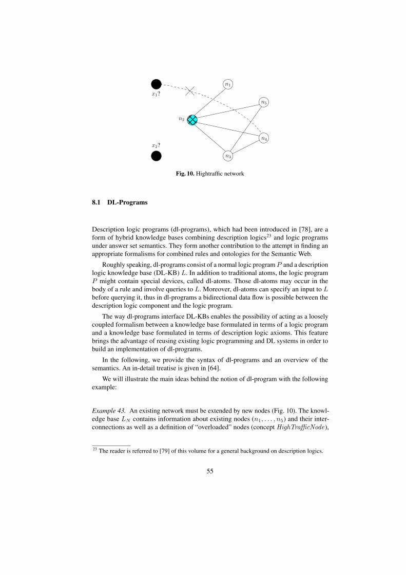
n1

x1?

x2?

n2

n3

n4

n5

Fig. 10. Hightraffic network

8.1 DL-Programs

Description logic programs (dl-programs), which had been introduced in [78], are aform of hybrid knowledge bases combining description logics23 and logic programsunder answer set semantics. They form another contribution to the attempt in finding anappropriate formalisms for combined rules and ontologies for the Semantic Web.

Roughly speaking, dl-programs consist of a normal logic programP and a descriptionlogic knowledge base (DL-KB) L. In addition to traditional atoms, the logic programP might contain special devices, called dl-atoms. Those dl-atoms may occur in thebody of a rule and involve queries to L. Moreover, dl-atoms can specify an input to Lbefore querying it, thus in dl-programs a bidirectional data flow is possible between thedescription logic component and the logic program.

The way dl-programs interface DL-KBs enables the possibility of acting as a looselycoupled formalism between a knowledge base formulated in terms of a logic programand a knowledge base formulated in terms of description logic axioms. This featurebrings the advantage of reusing existing logic programming and DL systems in order tobuild an implementation of dl-programs.

In the following, we provide the syntax of dl-programs and an overview of thesemantics. An in-detail treatise is given in [64].

We will illustrate the main ideas behind the notion of dl-program with the followingexample:

Example 43. An existing network must be extended by new nodes (Fig. 10). The knowl-edge base LN contains information about existing nodes (n1, . . . , n5) and their inter-connections as well as a definition of “overloaded” nodes (concept HighTrafficNode),

23 The reader is referred to [79] of this volume for a general background on description logics.

55

which are nodes with more than three connections:

≥ 1 wired v Node; > v ∀wired .Node; wired = wired−;

≥ 4 wired v HighTrafficNode; n1 6= n2 6= n3 6= n4 6= n5;

Node(n1); Node(n2); Node(n3); Node(n4); Node(n5);

wired(n1, n2); wired(n2, n3); wired(n2, n4);

wired(n2, n5); wired(n3, n4); wired(n3, n5).

In LN , only n2 is an overloaded node, and is highlighted in Fig. 10 with a criss-crosspattern.

To evaluate possible combinations of connecting the new nodes, the followingprogram PN is specified:

newnode(x1 ). (29)newnode(x2 ). (30)

overloaded(X)← DL[wired ] connect ; HighTrafficNode](X). (31)connect(X,Y )← newnode(X),DL[Node](Y ), (32)

not overloaded(Y ),not excl(X,Y ).

excl(X,Y )← connect(X,Z),DL[Node](Y ), Y 6= Z. (33)excl(X,Y )← connect(Z, Y ),newnode(Z),newnode(X), Z 6= X. (34)

excl(x1 , n4). (35)

Rules (29)–(30) define the new nodes to be added. Rule (31) imports knowledge aboutoverloaded nodes in the existing network, taking new connections already into account.Rule (32) connects a new node to an existing one, provided the latter is not overloadedand the connection is not to be disallowed, which is specified by Rule (33) (there mustnot be more than one connection for each new node) and Rule (34) (two new nodescannot be connected to the same existing one). Rule (35) states a specific condition:Node x1 must not be connected with n4.

Two different semantics have been defined for dl-programs, the (strong) answer-setsemantics [78] and the well-founded semantics [80, 81]. The former extends the notionof Gelfond-Lifschitz reduct (see Section 4) incorporating the presence of dl-atoms: dl-programs can have, in general, multiple answer sets. The latter extends the well-foundedsemantics of [22] to dl-programs.

Example 44. As specified by the strong answer set semantics of dl-programs, the pro-gram (LN , PN ) in Example 43 has four strong answer sets (we show only atomswith predicate connect): M1 = {connect(x1, n1), connect(x2, n4), . . . }, M2 ={connect(x1, n1), connect(x2, n5), . . . }, M3 = {connect(x1, n5), connect(x2, n1),. . . }, and M4 = {connect(x1, n5), connect(x2, n4), . . . }. Note that the ground dl-atom

DL[wired ] connect ; HighTrafficNode](n2)

from rule (31) is true in any partial interpretation of PN . According to the proposedwell-founded semantics for dl-programs in [80], the unique well-founded model of(LN , PN ) contains thus overloaded(n2 ).

56

Features and Properties of DL-Programs. The strong answer set semantics of dl-programs is nonmonotonic, and generalizes the stable semantics of ordinary logic pro-grams. In particular, satisfiable positive dl-programs (programs without default negationand −∩ operator) have a least model semantics, and satisfiable stratified dl-programs havea unique minimal model which is iteratively described by a finite sequence of leastmodels.

Applications. The bidirectional flow of knowledge between a description logic baseand a logic program component enables a variety of possibilities. A major applicationfor dl-programs is nonmonotonic reasoning on top of monotonic systems. It is forinstance possible to take a dl-knowledge base L and coupling it with a properly designedlogic program in order to extend L with defaults [38] and closed world assumption(CWA) [37]. Both reasoning applications can be implemented in dl-programs to supportnonmonotonic reasoning for description logics, as detailed in [64].

8.2 HEX-Programs

HEX-programs [82] are declarative nonmonotonic logic programs with support forexternal knowledge and higher-order disjunctive rules, under answer set semantics. Inspirit of dl-programs, they allow for a loose coupling between general external knowledgesources and declarative logic programs through the notion of external atoms, whichtake input from the logic program and exchange inferences with the external source. Inaddition, meta-reasoning tasks may be accomplished by means of higher-order atoms.HEX-programs are evaluated under a generalized answer-set semantics, thus are inprinciple capable of capturing many proposed extensions in answer-set programming.

Syntax of HEX-Programs. Let C, X , and G be mutually disjoint sets whose elementsare called constant names, variable names, and external predicate names, respectively.Unless explicitly specified, elements from X (resp., C) are denoted with first letter inupper case (resp., lower case), while elements from G are prefixed with the “&” symbol.We note that constant names serve both as individual and predicate names.

Elements from C ∪ X are called terms. A higher-order atom (or atom) is a tuple(Y0, Y1, . . . , Yn), where Y0, . . . , Yn are terms; n ≥ 0 is the arity of the atom. Intuitively,Y0 is the predicate name, and we thus also use the more familiar notation Y0(Y1, . . . , Yn).The atom is ordinary, if Y0 is a constant.

For example, (x, rdf :type, c), node(X), and D(a, b), are atoms; the first two areordinary atoms.

An external atom is of the form

&g [Y1, . . . , Yn](X1, . . . , Xm) , (36)

where Y1, . . . , Yn and X1, . . . , Xm are two lists of terms (called input and output lists,respectively), and &g ∈ G is an external predicate name. We assume that &g hasfixed lengths in(&g) = n and out(&g) = m for input and output lists, respectively.Intuitively, an external atom provides a way for deciding the truth value of an outputtuple depending on the extension of a set of input predicates: in this respect, an externalpredicate &g is equipped with a function f&g evaluating to true for proper input values.

57

subRelation(brotherOf , relativeOf ). (38)

brotherOf (john, al). (39)

relativeOf (john, joe). (40)

brotherOf (al ,mick). (41)

invites(john, X) ∨ skip(X)← X 6= john,&reach[relativeOf , john](X). (42)

R(X,Y )← subRelation(P,R), P (X,Y ). (43)

someInvited ← invites(john, X). (44)

← not someInvited . (45)

← &degs[invites](Min,Max ),Max > 2. (46)

Fig. 11. Example HEX program

A rule r is of the form

α1 ∨ · · · ∨ αk ← β1, . . . , βm,notβm+1, . . . ,notβn , (37)

where m, k ≥ 0, α1, . . . , αk are atoms, and β1, . . . , βn are either atoms or externalatoms. We define H(r) = {α1, . . . , αk} and B(r) = B+(r) ∪B−(r), where B+(r) ={β1, . . . , βm} and B−(r) = {βm+1, . . . , βn}. If H(r) = ∅ and B(r) 6= ∅, then r is aconstraint, and if B(r) = ∅ and H(r) 6= ∅, then r is a fact; r is ordinary, if it containsonly ordinary atoms. A HEX-program is a finite set P of rules. It is ordinary, if all rulesare ordinary.

We next give an illustrative example.

Example 45 ([83]). Consider the HEX-program P in Figure 11. Informally, this programrandomly selects a certain number of John’s relatives for invitation. The first line statesthat brotherOf is a subrelation of relativeOf , and the next three lines give concrete facts.The disjunctive rule (42) chooses relatives, employing the external predicate &reach.This latter predicate takes in input a binary relation e and a node name n, returning thenodes reachable from n when traversing the graph described by e (see the followingExample 47). Rule (43) axiomatizes subrelation inclusion exploiting higher-order atoms;that is, for those couples of binary predicates p, r for which it holds subRelation(p, r),it must be that r(x, y) holds whenever p(x, y) is true.

The constraints (45) and (46) ensure that the number of invitees is between 1 and 2,using (for illustration) an external predicate &degs from a graph library. Such a predicatehas a valuation function f&degs where f&degs(I, e,min,max ) is true iff min and maxare, respectively, the minimum and maximum vertex degree of the graph induced by theedges contained in the extension of predicate e in interpretation I .

Semantics of HEX-Programs. In the sequel, let P be a HEX-program. The Herbrandbase of P , denoted HBP , is the set of all possible ground versions of atoms and externalatoms occurring in P obtained by replacing variables with constants from C. Thegrounding of a rule r, grnd(r), is defined accordingly, and the grounding of program

58

P is given by grnd(P ) =⋃r∈P grnd(r). Unless specified otherwise, C, X , and G are

implicitly given by P .

Example 46 ([83]). Given C = {edge, arc, a, b}, ground instances of E(X, b) arefor instance edge(a, b), arc(a, b), a(edge, b), and arc(arc, b). Ground instances of&reach[edge, N ](X) are all possible combinations where N and X are replaced byelements from C; some examples are &reach[edge, edge](a), &reach[edge, arc](b),and &reach[edge, edge](edge).

An interpretation relative to P is any subset I ⊆ HBP containing only atoms. Wesay that I is a model of atom a ∈ HBP , denoted I |= a, if a ∈ I .

With every external predicate name &g ∈ G, we associate an (n+m+1)-ary Booleanfunction f&g assigning each tuple (I, y1 . . . , yn, x1, . . . , xm) either 0 or 1, where n =in(&g), m = out(&g), I ⊆ HBP , and xi, yj ∈ C. We say that I ⊆ HBP is a model ofa ground external atom a = &g [y1, . . . , yn](x1, . . . , xm), denoted I |= a, if and only iff&g(I, y1, . . . , yn, x1, . . . , xm) = 1.

Example 47 ([83]). Let us associate with the external atom &reach a function f&reachsuch that f&reach(I, E,A,B) = 1 iff B is reachable in the graph E from A. Let I ={e(b, c), e(c, d)}. Then, I is a model of &reach[e, b](d) since f&reach(I, e, b, d) = 1.

Note that in contrast to the semantics of higher-order atoms, which in essence reducesto first-order logic as customary (cf. [84]), the semantics of external atoms is in spirit ofsecond order logic since it involves predicate extensions.

Considering example 45, as John’s relatives are determined to be Al, Joe, and Mick,P has six answer sets, each of which contains one or two of the facts invites(john, al),invites(john, joe), and invites(john,mick).

Let r be a ground rule. We define (i) I |= H(r) iff there is some a ∈ H(r) suchthat I |= a, (ii) I |=B(r) iff I |= a for all a ∈ B+(r) and I 6|= a for all a ∈ B−(r), and(iii) I |= r iff I |=H(r) whenever I |=B(r). We say that I is a model of a HEX-programP , denoted I |= P , iff I |= r for all r ∈ grnd(P ). We call P satisfiable, if it has somemodel.

Given a HEX-program P , the FLP-reduct of P with respect to I ⊆ HBP , de-noted fPI , is the set of all r ∈ grnd(P ) such that I |= B(r). I ⊆ HBP is an answer setof P iff I is a minimal model of fPI .

In principle, the truth value of an external atom depends on its input and output listsand on the entire model of the program. In practice, however, we can identify certaintypes of input terms that allow to restrict the input interpretation to specific relations. TheBoolean function associated with the external atom &reach[edge, a](X) for instancewill only consider the extension of the predicate edge and the constant value a forcomputing its result, and simply ignore everything else of the given input interpretation.

Features and Properties of HEX-Programs. As mentioned above, HEX-programsare a generalization of dl-programs, consisting indeed in a form of coupling of ruleswith arbitrary external computation sources, within a declarative logic-based setting.The higher-order features are similar to those of HiLog [85], i.e., the semantics of thishigh-order extension is still within first-order logic.

59

The semantics of HEX-programs conservatively extends ordinary answer-set pro-grams, and it is easily extendable to support weak constraints [86]. External predicatescan define other ASP features like aggregate functions [61]. Computational complexityof the language depends on external functions. The former is however not affected ifexternal functions evaluate in polynomial time.

The dlvhex prototype,24 an implementation of HEX-programs, is based on a flexibleand modular architecture. The evaluation of the external atoms is realized by plugins,which are loaded at run-time. The pool of available external predicates can be easilycustomized by third-party developers.

Applications. HEX-programs have been put to use in many applications in differentcontexts. Hoehndorf et al. [70] showed how to combine multiple biomedical upperontologies by extending the first-order semantics of terminological knowledge withdefault logic. The corresponding prototype implementation of such kind of system isgiven by mapping the default rules to HEX-program. Fuzzy extensions of answer-setprograms and their relationship to HEX-programs are given in [87, 88]. The formermaps fuzzy answer set programs to HEX-programs, whereas the latter defines a fuzzysemantics for HEX-programs and gives a translation to standard HEX-programs. In [89],the planning language Kc has been introduced which features external function calls inspirit of HEX-programs.

8.3 Other linguistic extension of ASP in the direction of Semantic Web

We briefly survey here other notable works aiming at integrating the stable model seman-tics with Semantic Web related formalisms, and remind the reader to other discussionsof related work such as [18, 71].

Research efforts can be categorized in the two main groups of translational ap-proaches and integration approaches. The latter can be further classified in loose, tightor full integration.

As for integration approaches, DL+log [90] is the latest in a chain of extensions ofthe DL ALC with rules such as AL-log , r- and r+-hybrid knowledge bases. As a tightsemantics approach, DL+log gives meaning to combined knowledge bases in termsof unique model structures, which aim at satisfying both the description logic base athand and the logic program. Hybrid MKNF knowledge bases [91] build on Lifschitz’sbimodal Logic of Minimal Knowledge and Negation as Failure (MKNF) [93], and aim ata seamless (which is sometimes referred as full integration) integration of classic andnonmonotonic semantics beyond tight integration approaches. Besides dl-programs andhex-programs, it is worth mentioning other loose coupling languages in the direction ofprobabilistic [94] and fuzzy hybrid systems [95] under stable semantics; see [73] for anoverview. An extension of RDF(S) with stable models has been proposed in [96].

One might also consider the idea of translating Semantic Web ontologies to semanti-cally equivalent ASP logic programs. This task is quite challenging, given the profoundsemantic differences between the two formalisms. Nonetheless, some success has beenreached, and translation from several flavors of description logics to ASP are known, cf.

24 http://www.kr.tuwien.ac.at/research/systems/dlvhex/

60

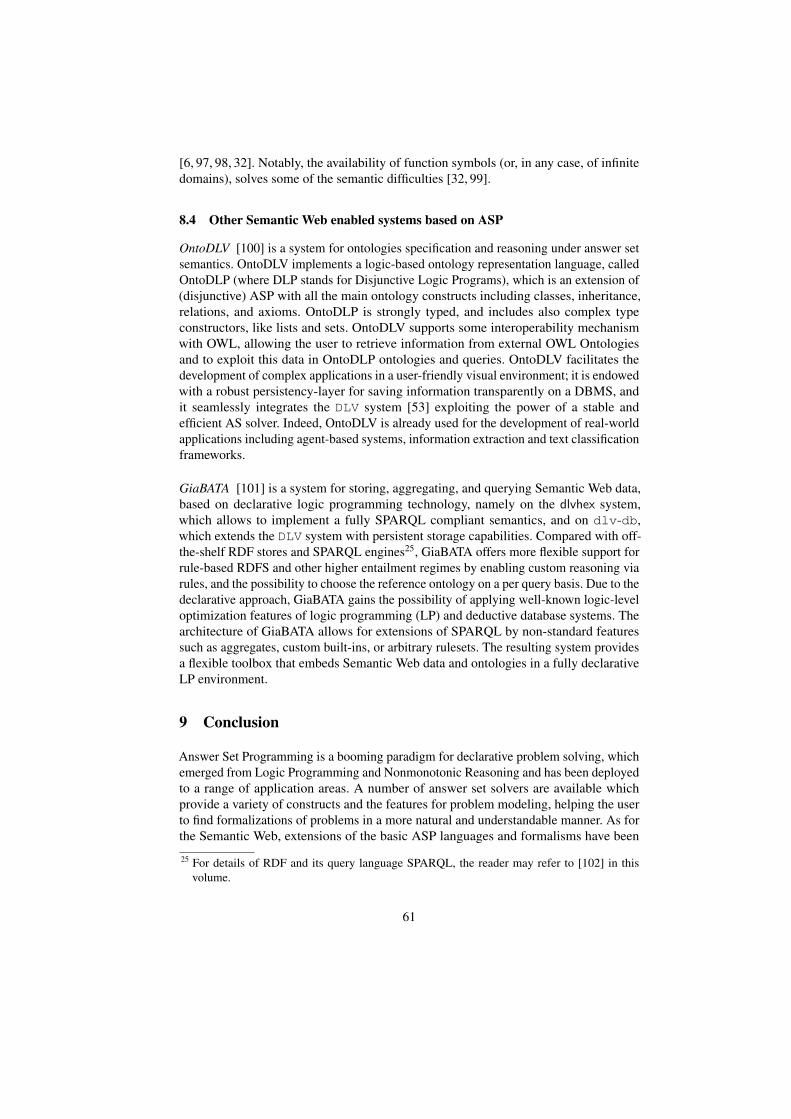
[6, 97, 98, 32]. Notably, the availability of function symbols (or, in any case, of infinitedomains), solves some of the semantic difficulties [32, 99].

8.4 Other Semantic Web enabled systems based on ASP

OntoDLV [100] is a system for ontologies specification and reasoning under answer setsemantics. OntoDLV implements a logic-based ontology representation language, calledOntoDLP (where DLP stands for Disjunctive Logic Programs), which is an extension of(disjunctive) ASP with all the main ontology constructs including classes, inheritance,relations, and axioms. OntoDLP is strongly typed, and includes also complex typeconstructors, like lists and sets. OntoDLV supports some interoperability mechanismwith OWL, allowing the user to retrieve information from external OWL Ontologiesand to exploit this data in OntoDLP ontologies and queries. OntoDLV facilitates thedevelopment of complex applications in a user-friendly visual environment; it is endowedwith a robust persistency-layer for saving information transparently on a DBMS, andit seamlessly integrates the DLV system [53] exploiting the power of a stable andefficient AS solver. Indeed, OntoDLV is already used for the development of real-worldapplications including agent-based systems, information extraction and text classificationframeworks.

GiaBATA [101] is a system for storing, aggregating, and querying Semantic Web data,based on declarative logic programming technology, namely on the dlvhex system,which allows to implement a fully SPARQL compliant semantics, and on dlv-db,which extends the DLV system with persistent storage capabilities. Compared with off-the-shelf RDF stores and SPARQL engines25, GiaBATA offers more flexible support forrule-based RDFS and other higher entailment regimes by enabling custom reasoning viarules, and the possibility to choose the reference ontology on a per query basis. Due to thedeclarative approach, GiaBATA gains the possibility of applying well-known logic-leveloptimization features of logic programming (LP) and deductive database systems. Thearchitecture of GiaBATA allows for extensions of SPARQL by non-standard featuressuch as aggregates, custom built-ins, or arbitrary rulesets. The resulting system providesa flexible toolbox that embeds Semantic Web data and ontologies in a fully declarativeLP environment.

9 Conclusion

Answer Set Programming is a booming paradigm for declarative problem solving, whichemerged from Logic Programming and Nonmonotonic Reasoning and has been deployedto a range of application areas. A number of answer set solvers are available whichprovide a variety of constructs and the features for problem modeling, helping the userto find formalizations of problems in a more natural and understandable manner. As forthe Semantic Web, extensions of the basic ASP languages and formalisms have been

25 For details of RDF and its query language SPARQL, the reader may refer to [102] in thisvolume.

61

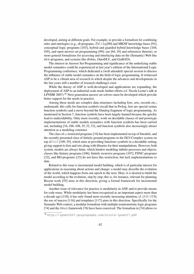
developed, aiming at different goals. For example, to provide a formalism for combiningrules and ontologies (e.g., dl-programs, DL+log[90] and MKNF knowledge bases [91],conceptual logic programs [103], hybrid and guarded hybrid knowledge bases [104,105], and open answer set programming [99]; see [64, 18] and references therein), ormore general formalisms for accessing and interfacing data on the (Semantic) Web likeHEX-programs, and systems like dlvhex, OntoDLV, and GiaBATA.

The interest in Answer Set Programming and significance of the underlying stablemodel semantics could be experienced at last year’s edition of the International LogicProgramming conference, which dedicated a (well-attended) special session to discussthe influence of stable model semantics on the field of logic programming. It witnessedASP to be a vibrant area of research in which despite the advances and developments inthe last years still a number of research challenges exist.

While the theory of ASP is well-developed and applications are expanding, thedeployment of ASP to an industrial scale needs further efforts (cf. Nicola Leone’s talk atLPNMR 2007).26 Next generation answer set solvers must be developed which providebetter support for the needs in practice.

Among these needs are complex data structures including lists, sets, records etc.;underneath, this calls for function symbols (recall that in Prolog, lists are special syntaxfunction symbols) and a move beyond the Datalog fragment of logic programming. Asmentioned in Section 7, function symbols have been largely banned because the quicklylead to undecidability. Only more recently, work on decidable classes of and prototypeimplementations of stable models semantics with function symbols has been carriedout, including [34, 106–108, 35, 32, 33], and function symbols also increasingly attractattention as a modeling construct.

The class of ω-restricted programs [34] has been implemented on top of Smodels, andthe recently presented class of finitely-ground programs in the DLV-Complex system ontop of DLV [109, 35], which aims at providing functions symbols in a decidable setting,giving support to lists and sets along with libraries for their manipulations. However, bothsystem, models are always finite, which hinders modeling infinite processes and objects;classes like finitary programs [106], finitely recursive programs [107], FDNC-programs[32], and BD-programs [33] do not have this restriction, but lack implementations todate.

Related to this issue is incremental model building, which is of particular interest forapplications in reasoning about actions and change: a model may describe the evolutionof the world, which happens from one epoch to the next. Here, it is desired to build themodel according to the evolution, step by step; this is, for instance, relevant for planning.Recent work [55] aims in this direction, giving a formal framework for incrementalmodel building.

Another issue of relevance for practice is modularity in ASP, and to provide meansfor code reuse. While modularity has been recognized as an important aspect more thana decade ago [110], it has only found more recently increasing attention, cf. [111–115];the use of macros [116] and templates [117] aims in this direction. Specifically for theSemantic Web context, a modular formalism with multiple nonmonotonic logic programs[74] and the MWeb framework [76] have been conceived. The formalism in [74] allows to

26 http://lpnmr2007.googlepages.com/nicola-lpnmr07.pdf

62

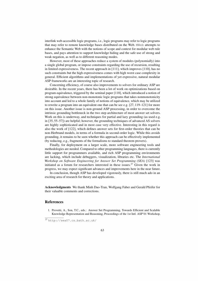
interlink web-accessible logic programs, i.e., logic programs may refer to logic programsthat may refer to remote knowledge bases distributed on the Web. MWeb attempts toenhance the Semantic Web with the notions of scope and context for modular web rulebases, and pays attention to support knowledge hiding and the safe use of strong andweak negation, as well as to different reasoning modes.

However, most of these approaches reduce a system of modules (polynomially) intoa single global program, or impose constraints regarding the use of recursion, resultingin limited expressiveness. The recent approach in [111], which improves [110], has nosuch constraints but the high expressiveness comes with high worst case complexity ingeneral. Efficient algorithms and implementations of yet expressive, natural modularASP frameworks are an interesting topic of research.

Concerning efficiency, of course also improvements to solvers for ordinary ASP aredesirable. In the recent years, there has been a lot of work on optimizations based onprogram equivalence, triggered by the seminal paper [118], which introduced a notion ofstrong equivalence between non-monotonic logic programs that takes nonmonotonicityinto account and led to a whole family of notions of equivalence, which may be utilizedto rewrite a program into an equivalent one that can be see e.g. [27, 119–121] for moreon this issue. Another issue is non-ground ASP processing, in order to overcome theintrinsic grounding bottleneck in the two step architecture of most answer set solvers.Work on this is underway, and techniques for partial and lazy grounding (as used e.g.in [35, 55–57]) are helpful; however, the grounding techniques of advanced AS solversare highly sophisticated and in most case very effective. Interesting in this regard isalso the work of [122], which defines answer sets for first-order theories that can benon-Herbrand models, in terms of a formula in second-order logic. While this avoidsgrounding, it remains to be seen whether this approach can be effectively implemented(by reducing, e.g., fragments of the formalisms to standard theorem provers).

Finally, for deployment on a larger scale, more software engineering tools andmethodologies are needed. Compared to other programming languages, there is currentlylittle support for programmers available, and rich ASP programming environmentsare lacking, which include debuggers, visualization, libraries etc. The InternationalWorkshop on Software Engineering for Answer Set Programming (SEA) [123] wasinitiated as a forum for researchers interested in these issues.27 Given the work inprogress, we may expect significant advances and improvements here in the near future.

In conclusion, though ASP has developed vigorously, there is still much ado in anexciting area of research for theory and applications.

Acknowledgments We thank Minh Dao-Tran, Wolfgang Faber and Gerald Pfeifer fortheir valuable comments and corrections.

References

1. Provetti, A., Son, T.C., eds.: Answer Set Programming, Towards Efficient and ScalableKnowledge Representation and Reasoning, Proceedings of the 1st Intl. ASP’01 Workshop,

27 http://sea07.cs.bath.ac.uk/

63

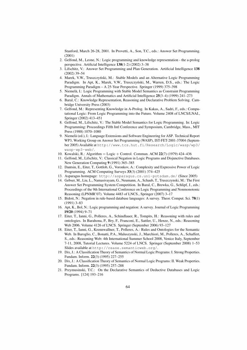
Stanford, March 26-28, 2001. In Provetti, A., Son, T.C., eds.: Answer Set Programming.(2001)

2. Gelfond, M., Leone, N.: Logic programming and knowledge representation - the a-prologperspective. Artificial Intelligence 138(1-2) (2002) 3–38

3. Lifschitz, V.: Answer Set Programming and Plan Generation. Artificial Intelligence 138(2002) 39–54

4. Marek, V.W., Truszczynski, M.: Stable Models and an Alternative Logic ProgrammingParadigm. In Apt, K., Marek, V.W., Truszczynski, M., Warren, D.S., eds.: The LogicProgramming Paradigm – A 25-Year Perspective. Springer (1999) 375–398

5. Niemela, I.: Logic Programming with Stable Model Semantics as Constraint ProgrammingParadigm. Annals of Mathematics and Artificial Intelligence 25(3–4) (1999) 241–273

6. Baral, C.: Knowledge Representation, Reasoning and Declarative Problem Solving. Cam-bridge University Press (2003)

7. Gelfond, M.: Representing Knowledge in A-Prolog. In Kakas, A., Sadri, F., eds.: Compu-tational Logic: From Logic Programming into the Future. Volume 2408 of LNCS/LNAI.,Springer (2002) 413–451

8. Gelfond, M., Lifschitz, V.: The Stable Model Semantics for Logic Programming. In: LogicProgramming: Proceedings Fifth Intl Conference and Symposium, Cambridge, Mass., MITPress (1988) 1070–1080

9. Niemela (ed.), I.: Language Extensions and Software Engineering for ASP. Technical ReportWP3, Working Group on Answer Set Programming (WASP), IST-FET-2001-37004 (Septem-ber 2005) Available at http://www.tcs.hut.fi/Research/Logic/wasp/wp3/wasp-wp3-web/.

10. Kowalski, R.: Algorithm = Logic + Control. Commun. ACM 22(7) (1979) 424–43611. Gelfond, M., Lifschitz, V.: Classical Negation in Logic Programs and Disjunctive Databases.

New Generation Computing 9 (1991) 365–38512. Dantsin, E., Eiter, T., Gottlob, G., Voronkov, A.: Complexity and Expressive Power of Logic

Programming. ACM Computing Surveys 33(3) (2001) 374–42513. Asparagus homepage: http://asparagus.cs.uni-potsdam.de/ (Since 2005)14. Gebser, M., Liu, L., Namasivayam, G., Neumann, A., Schaub, T., Truszczynski, M.: The First

Answer Set Programming System Competition. In Baral, C., Brewka, G., Schlipf, J., eds.:Proceedings of the 9th International Conference on Logic Programming and NonmonotonicReasoning (LPNMR’07). Volume 4483 of LNCS., Springer (2007) 3–17

15. Bidoit, N.: Negation in rule-based database languages: A survey. Theor. Comput. Sci. 78(1)(1991) 3–83

16. Apt, K., Bol, N.: Logic programming and negation: A survey. Journal of Logic Programming19/20 (1994) 9–71

17. Eiter, T., Ianni, G., Polleres, A., Schindlauer, R., Tompits, H.: Reasoning with rules andontologies. In Barahona, P., Bry, F., Franconi, E., Sattler, U., Henze, N., eds.: ReasoningWeb 2006. Volume 4126 of LNCS. Springer (September 2006) 93–127

18. Eiter, T., Ianni, G., Krennwallner, T., Polleres, A.: Rules and Ontologies for the SemanticWeb. In Baroglio, C., Bonatti, P.A., Maluszynski, J., Marchiori, M., Polleres, A., Schaffert,S., eds.: Reasoning Web: 4th International Summer School 2008, Venice Italy, September7-11, 2008, Tutorial Lectures. Volume 5224 of LNCS. Springer (September 2008) 1–53Slides available at http://rease.semanticweb.org/.

19. Dix, J.: A Classification Theory of Semantics of Normal Logic Programs: I. Strong Properties.Fundam. Inform. 22(3) (1995) 227–255

20. Dix, J.: A Classification Theory of Semantics of Normal Logic Programs: II. Weak Properties.Fundam. Inform. 22(3) (1995) 257–288

21. Przymusinski, T.C.: On the Declarative Semantics of Deductive Databases and LogicPrograms. [124] 193–216

64

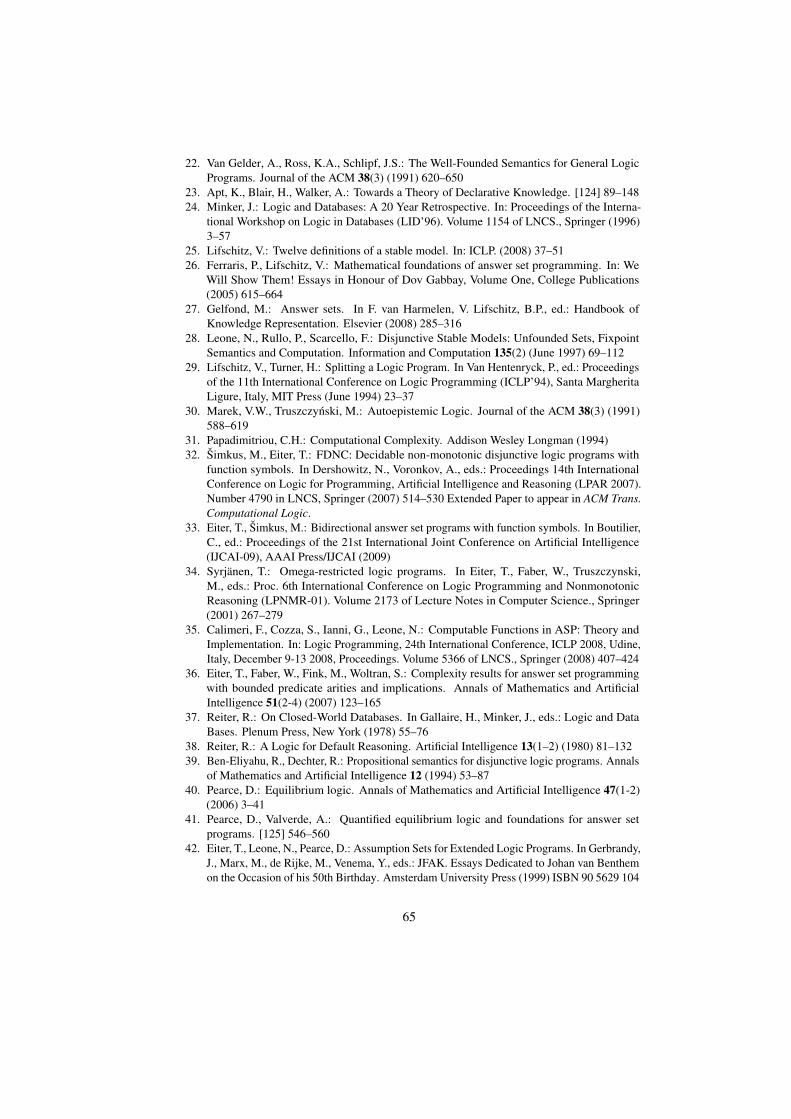
22. Van Gelder, A., Ross, K.A., Schlipf, J.S.: The Well-Founded Semantics for General LogicPrograms. Journal of the ACM 38(3) (1991) 620–650

23. Apt, K., Blair, H., Walker, A.: Towards a Theory of Declarative Knowledge. [124] 89–14824. Minker, J.: Logic and Databases: A 20 Year Retrospective. In: Proceedings of the Interna-

tional Workshop on Logic in Databases (LID’96). Volume 1154 of LNCS., Springer (1996)3–57

25. Lifschitz, V.: Twelve definitions of a stable model. In: ICLP. (2008) 37–5126. Ferraris, P., Lifschitz, V.: Mathematical foundations of answer set programming. In: We

Will Show Them! Essays in Honour of Dov Gabbay, Volume One, College Publications(2005) 615–664

27. Gelfond, M.: Answer sets. In F. van Harmelen, V. Lifschitz, B.P., ed.: Handbook ofKnowledge Representation. Elsevier (2008) 285–316

28. Leone, N., Rullo, P., Scarcello, F.: Disjunctive Stable Models: Unfounded Sets, FixpointSemantics and Computation. Information and Computation 135(2) (June 1997) 69–112

29. Lifschitz, V., Turner, H.: Splitting a Logic Program. In Van Hentenryck, P., ed.: Proceedingsof the 11th International Conference on Logic Programming (ICLP’94), Santa MargheritaLigure, Italy, MIT Press (June 1994) 23–37

30. Marek, V.W., Truszczynski, M.: Autoepistemic Logic. Journal of the ACM 38(3) (1991)588–619

31. Papadimitriou, C.H.: Computational Complexity. Addison Wesley Longman (1994)32. Simkus, M., Eiter, T.: FDNC: Decidable non-monotonic disjunctive logic programs with

function symbols. In Dershowitz, N., Voronkov, A., eds.: Proceedings 14th InternationalConference on Logic for Programming, Artificial Intelligence and Reasoning (LPAR 2007).Number 4790 in LNCS, Springer (2007) 514–530 Extended Paper to appear in ACM Trans.Computational Logic.

33. Eiter, T., Simkus, M.: Bidirectional answer set programs with function symbols. In Boutilier,C., ed.: Proceedings of the 21st International Joint Conference on Artificial Intelligence(IJCAI-09), AAAI Press/IJCAI (2009)

34. Syrjanen, T.: Omega-restricted logic programs. In Eiter, T., Faber, W., Truszczynski,M., eds.: Proc. 6th International Conference on Logic Programming and NonmonotonicReasoning (LPNMR-01). Volume 2173 of Lecture Notes in Computer Science., Springer(2001) 267–279

35. Calimeri, F., Cozza, S., Ianni, G., Leone, N.: Computable Functions in ASP: Theory andImplementation. In: Logic Programming, 24th International Conference, ICLP 2008, Udine,Italy, December 9-13 2008, Proceedings. Volume 5366 of LNCS., Springer (2008) 407–424

36. Eiter, T., Faber, W., Fink, M., Woltran, S.: Complexity results for answer set programmingwith bounded predicate arities and implications. Annals of Mathematics and ArtificialIntelligence 51(2-4) (2007) 123–165

37. Reiter, R.: On Closed-World Databases. In Gallaire, H., Minker, J., eds.: Logic and DataBases. Plenum Press, New York (1978) 55–76

38. Reiter, R.: A Logic for Default Reasoning. Artificial Intelligence 13(1–2) (1980) 81–13239. Ben-Eliyahu, R., Dechter, R.: Propositional semantics for disjunctive logic programs. Annals

of Mathematics and Artificial Intelligence 12 (1994) 53–8740. Pearce, D.: Equilibrium logic. Annals of Mathematics and Artificial Intelligence 47(1-2)

(2006) 3–4141. Pearce, D., Valverde, A.: Quantified equilibrium logic and foundations for answer set

programs. [125] 546–56042. Eiter, T., Leone, N., Pearce, D.: Assumption Sets for Extended Logic Programs. In Gerbrandy,

J., Marx, M., de Rijke, M., Venema, Y., eds.: JFAK. Essays Dedicated to Johan van Benthemon the Occasion of his 50th Birthday. Amsterdam University Press (1999) ISBN 90 5629 104

65

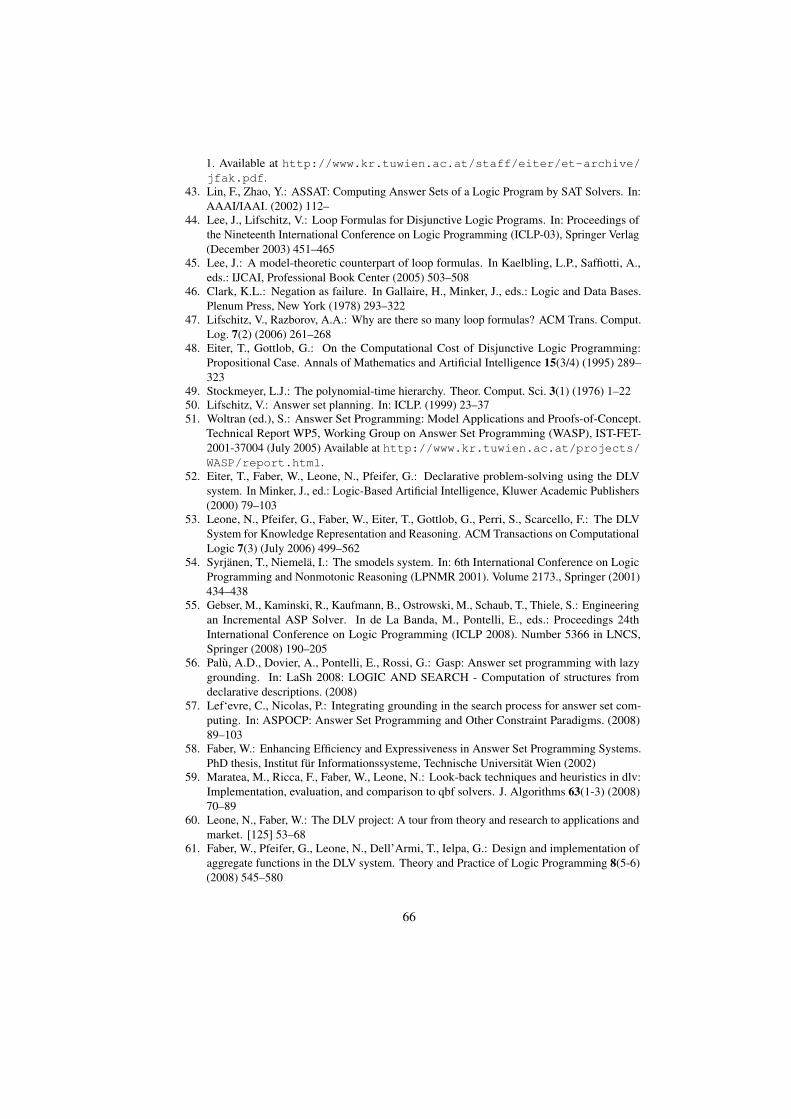
1. Available at http://www.kr.tuwien.ac.at/staff/eiter/et-archive/jfak.pdf.

43. Lin, F., Zhao, Y.: ASSAT: Computing Answer Sets of a Logic Program by SAT Solvers. In:AAAI/IAAI. (2002) 112–

44. Lee, J., Lifschitz, V.: Loop Formulas for Disjunctive Logic Programs. In: Proceedings ofthe Nineteenth International Conference on Logic Programming (ICLP-03), Springer Verlag(December 2003) 451–465

45. Lee, J.: A model-theoretic counterpart of loop formulas. In Kaelbling, L.P., Saffiotti, A.,eds.: IJCAI, Professional Book Center (2005) 503–508

46. Clark, K.L.: Negation as failure. In Gallaire, H., Minker, J., eds.: Logic and Data Bases.Plenum Press, New York (1978) 293–322

47. Lifschitz, V., Razborov, A.A.: Why are there so many loop formulas? ACM Trans. Comput.Log. 7(2) (2006) 261–268

48. Eiter, T., Gottlob, G.: On the Computational Cost of Disjunctive Logic Programming:Propositional Case. Annals of Mathematics and Artificial Intelligence 15(3/4) (1995) 289–323

49. Stockmeyer, L.J.: The polynomial-time hierarchy. Theor. Comput. Sci. 3(1) (1976) 1–2250. Lifschitz, V.: Answer set planning. In: ICLP. (1999) 23–3751. Woltran (ed.), S.: Answer Set Programming: Model Applications and Proofs-of-Concept.

Technical Report WP5, Working Group on Answer Set Programming (WASP), IST-FET-2001-37004 (July 2005) Available at http://www.kr.tuwien.ac.at/projects/WASP/report.html.

52. Eiter, T., Faber, W., Leone, N., Pfeifer, G.: Declarative problem-solving using the DLVsystem. In Minker, J., ed.: Logic-Based Artificial Intelligence, Kluwer Academic Publishers(2000) 79–103

53. Leone, N., Pfeifer, G., Faber, W., Eiter, T., Gottlob, G., Perri, S., Scarcello, F.: The DLVSystem for Knowledge Representation and Reasoning. ACM Transactions on ComputationalLogic 7(3) (July 2006) 499–562

54. Syrjanen, T., Niemela, I.: The smodels system. In: 6th International Conference on LogicProgramming and Nonmotonic Reasoning (LPNMR 2001). Volume 2173., Springer (2001)434–438

55. Gebser, M., Kaminski, R., Kaufmann, B., Ostrowski, M., Schaub, T., Thiele, S.: Engineeringan Incremental ASP Solver. In de La Banda, M., Pontelli, E., eds.: Proceedings 24thInternational Conference on Logic Programming (ICLP 2008). Number 5366 in LNCS,Springer (2008) 190–205

56. Palu, A.D., Dovier, A., Pontelli, E., Rossi, G.: Gasp: Answer set programming with lazygrounding. In: LaSh 2008: LOGIC AND SEARCH - Computation of structures fromdeclarative descriptions. (2008)

57. Lef‘evre, C., Nicolas, P.: Integrating grounding in the search process for answer set com-puting. In: ASPOCP: Answer Set Programming and Other Constraint Paradigms. (2008)89–103

58. Faber, W.: Enhancing Efficiency and Expressiveness in Answer Set Programming Systems.PhD thesis, Institut fur Informationssysteme, Technische Universitat Wien (2002)

59. Maratea, M., Ricca, F., Faber, W., Leone, N.: Look-back techniques and heuristics in dlv:Implementation, evaluation, and comparison to qbf solvers. J. Algorithms 63(1-3) (2008)70–89

60. Leone, N., Faber, W.: The DLV project: A tour from theory and research to applications andmarket. [125] 53–68

61. Faber, W., Pfeifer, G., Leone, N., Dell’Armi, T., Ielpa, G.: Design and implementation ofaggregate functions in the DLV system. Theory and Practice of Logic Programming 8(5-6)(2008) 545–580

66

62. Buccafurri, F., Faber, W., Leone, N.: Disjunctive logic programs with inheritance. Theoryand Practice of Logic Programming 2(3) (2002)

63. Eiter, T.: Answer set programming for the Semantic Web (tutorial). In Niemela, I., Dahl,V., eds.: Proceedings 23rd International Conference on Logic Programming (ICLP 2007).Number 4670 in LNCS, Springer (2007) 23–26 Slides available at http://www.dcc.fc.up.pt/iclp07/eiter.pdf.

64. Eiter, T., Ianni, G., Lukasiewicz, T., Schindlauer, R., Tompits, H.: Combining AnswerSet Programming with Description Logics for the Semantic Web. Artificial Intelligence172(12-13) (2008) 1495–1539

65. Polleres, A.: From SPARQL to rules (and back). In: Proceedings of the 16th InternationalConference on World Wide Web (WWW), ACM (2007) 787–796

66. Rainer, A.: Web Service Composition under Answer Set Programming. In: Proc. KI 2005Workshop ”Planen, Scheduling und Konfigurieren, Entwerfen” (PuK 2005). (2005)

67. Pontelli, E., Son, T.C., Baral, C.: A framework for composition and inter-operation of rulesin the semantic web. In Eiter, T., Franconi, E., Hodgson, R., Stephens, S., eds.: RuleML,IEEE Computer Society (2006) 39–50

68. Friedrich et al., G.: Model-based repair of web service processes. Technical Report 2008/001,ISBI research group, University of Klagenfurt (2008) http://test-informations.info/.

69. Eiter, T., Ianni, G., Schindlauer, R., Tompits, H., Wang, K.: Forgetting in managing rulesand ontologies. In: IEEE/WIC/ACM International Conference on Web Intelligence (WI2006), Hongkong, Dec. 2006, IEEE Computer Society (2006) 411–419 Preliminary versionat ALPSWS 2006.

70. Hoehndorf, R., Loebe, F., Kelso, J., Herre, H.: Representing default knowledge in biomedicalontologies: Application to the integration of anatomy and phenotype ontologies. BMCBioinformatics 8(1) (2007) 377

71. de Bruijn, J., Eiter, T., Polleres, A., Tompits, H.: On representational issues about combi-nations of classical theories with nonmonotonic rules. In Lang, J., Lin, F., Wang, J., eds.:KSEM. Volume 4092 of Lecture Notes in Computer Science., Springer (2006) 1–22

72. Denecker, M., Ternovska, E.: A logic of non-monotone inductive definitions. ACM Transac-tions on Computational Logic 9(2:14) (2008)

73. Drabent, W., Eiter, T., Ianni, G., Krennwallner, T., Lukasiewicz, T., Małuszynski, J.: Hybridreasoning with rules and ontologies. In Bry, F., Małuszynski, J., eds.: Semantic Techniquesfor the Web: The REWERSE perspective. Number 5500 in LNCS. Springer (2009) 50 pp.To appear.

74. Polleres, A., Feier, C., Harth, A.: Rules with Contextually Scoped Negation. In: Proceedingsof the 3rd European Conference on Semantic Web (ESWC 2006). Volume 4011 of LNCS.,Springer (2006) 332–347

75. Damasio, C.V., Analyti, A., Antoniou, G., Wagner, G.: Supporting open and closed worldreasoning on the web. In Alferes, J.J., Bailey, J., May, W., Schwertel, U., eds.: PPSWR.Volume 4187 of Lecture Notes in Computer Science., Springer (2006) 149–163

76. Analyti, A., Antoniou, G., Damasio, C.V.: A principled framework for modular web rulebases and its semantics. In: Proceedings of the 11th International Conference on Principlesof Knowledge Representation and Reasoning (KR2008), AAAI Press (September 2008)

77. Alferes, J.J., Amador, R., May, W.: A general language for evolution and reactivity in thesemantic web. In Fages, F., Soliman, S., eds.: PPSWR. Volume 3703 of Lecture Notes inComputer Science., Springer (2005) 101–115

78. Eiter, T., Lukasiewicz, T., Schindlauer, R., Tompits, H.: Combining answer set programmingwith description logics for the Semantic Web. In Dubois, D., Welty, C., Williams, M.A., eds.:Proceedings Ninth International Conference on Principles of Knowledge Representation and

67

Reasoning (KR 2004), June 2-5, Whistler, British Columbia, Canada, Morgan Kaufmann(2004) 141–151

79. Baader, F.: Description logics. [126]80. Eiter, T., Lukasiewicz, T., Schindlauer, R., Tompits, H.: Well-founded semantics for descrip-

tion logic programs in the Semantic Web. In: Proceedings RuleML-2004. Volume 3323 ofLNCS., Springer (2004) 81–97

81. Eiter, T., Ianni, G., Lukasiewicz, T., Schindlauer, R.: Well-founded semantics for descriptionlogic programs in the Semantic Web. Technical Report INFSYS RR-1843-09-01, Institut furInformationssysteme, Technische Universitat Wien, A-1040 Vienna, Austria (March 2009)

82. Eiter, T., Ianni, G., Schindlauer, R., Tompits, H.: Effective integration of declarative ruleswith external evaluations for semantic web reasoning. In Sure, Y., Domingue, J., eds.:Proceedings 3rd European Conference on Semantic Web (ESWC 2006). Number 4011 inLNCS, Springer (2006) 273–287

83. Eiter, T., Ianni, G., Schindlauer, R., Tompits, H.: A Uniform Integration of Higher-OrderReasoning and External Evaluations in Answer Set Programming. In: International JointConference on Artificial Intelligence (IJCAI) 2005, Edinburgh, UK (August 2005) 90–96

84. Ross, K.A.: Modular stratification and magic sets for datalog programs with negation.Journal of the ACM 41(6) (1994) 1216–1266

85. Chen, W., Kifer, M., Warren, D.S.: Hilog: A foundation for higher-order logic programming.Journal of Logic Programming 15(3) (February 1993) 187–230

86. Buccafurri, F., Leone, N., Rullo, P.: Strong and Weak Constraints in Disjunctive Datalog. InDix, J., Furbach, U., Nerode, A., eds.: Proceedings of the 4th International Conference onLogic Programming and Non-Monotonic Reasoning (LPNMR’97). Volume 1265 of LectureNotes in AI (LNAI)., Dagstuhl, Germany, Springer Verlag (July 1997) 2–17

87. Nieuwenborgh, D.V., Cock, M.D., Vermeir, D.: Computing Fuzzy Answer Sets Using dlvhex.In Dahl, V., Niemela, I., eds.: Proceedings of the 23rd International Conference on LogicProgramming (ICLP 2007), Porto, Portugal, September 8-13, 2007. Volume 4670 of LNCS.,Springer (2007) 449–450

88. Heymans, S., Toma, I.: Ranking Services Using Fuzzy HEX-Programs. In Calvanese, D.,Lausen, G., eds.: Proceedings of the 2nd International Conference on Web Reasoning andRule Systems (RR 2008), Karlsruhe, Germany, October 31-November 1, 2008. Volume 5341of LNCS., Springer (2008) 181–196

89. Nieuwenborgh, D.V., Eiter, T., Vermeir, D.: Conditional Planning with External Functions.In Baral, C., Brewka, G., Schlipf, J.S., eds.: Proceedings of the 9th International Conferenceon Logic Programming and Nonmonotonic Reasoning (LPNMR 2007). Volume 4483 ofLNCS., Springer (2007) 214–227

90. Rosati, R.: DL+log: Tight Integration of Description Logics and Disjunctive Datalog. In:Proceedings of the Tenth International Conference on Principles of Knowledge Representa-tion and Reasoning (KR 2006), AAAI Press (2006) 68–78

91. Motik, B., Rosati, R.: A faithful integration of description logics with logic programming. In:IJCAI 2007, Proceedings of the 20th International Joint Conference on Artificial Intelligence.(2007) 477–482

92. Motik, B., et al. (ed.): OWL 2 Web Ontology Language Profiles. W3C (2009), http://www.w3.org/TR/owl-profiles/

93. Lifschitz, V.: Nonmonotonic databases and epistemic queries. In: Proceedings IJCAI-91.(1991) 381–386

94. Lukasiewicz, T.: Probabilistic description logic programs. Int. J. Approx. Reasoning 45(2)(2007) 288–307

95. Lukasiewicz, T., Straccia, U.: Description logic programs under probabilistic uncertainty andfuzzy vagueness. In: Symbolic and Quantitative Approaches to Reasoning with Uncertainty,9th European Conference, ECSQARU. (2007) 187–198

68

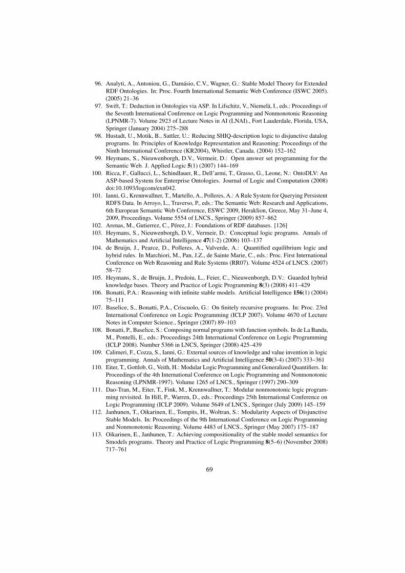
96. Analyti, A., Antoniou, G., Damasio, C.V., Wagner, G.: Stable Model Theory for ExtendedRDF Ontologies. In: Proc. Fourth International Semantic Web Conference (ISWC 2005).(2005) 21–36

97. Swift, T.: Deduction in Ontologies via ASP. In Lifschitz, V., Niemela, I., eds.: Proceedings ofthe Seventh International Conference on Logic Programming and Nonmonotonic Reasoning(LPNMR-7). Volume 2923 of Lecture Notes in AI (LNAI)., Fort Lauderdale, Florida, USA,Springer (January 2004) 275–288

98. Hustadt, U., Motik, B., Sattler, U.: Reducing SHIQ-description logic to disjunctive datalogprograms. In: Principles of Knowledge Representation and Reasoning: Proceedings of theNinth International Conference (KR2004), Whistler, Canada. (2004) 152–162

99. Heymans, S., Nieuwenborgh, D.V., Vermeir, D.: Open answer set programming for theSemantic Web. J. Applied Logic 5(1) (2007) 144–169

100. Ricca, F., Gallucci, L., Schindlauer, R., Dell’armi, T., Grasso, G., Leone, N.: OntoDLV: AnASP-based System for Enterprise Ontologies. Journal of Logic and Computation (2008)doi:10.1093/logcom/exn042.

101. Ianni, G., Krennwallner, T., Martello, A., Polleres, A.: A Rule System for Querying PersistentRDFS Data. In Arroyo, L., Traverso, P., eds.: The Semantic Web: Research and Applications,6th European Semantic Web Conference, ESWC 2009, Heraklion, Greece, May 31–June 4,2009, Proceedings. Volume 5554 of LNCS., Springer (2009) 857–862

102. Arenas, M., Gutierrez, C., Perez, J.: Foundations of RDF databases. [126]103. Heymans, S., Nieuwenborgh, D.V., Vermeir, D.: Conceptual logic programs. Annals of

Mathematics and Artificial Intelligence 47(1-2) (2006) 103–137104. de Bruijn, J., Pearce, D., Polleres, A., Valverde, A.: Quantified equilibrium logic and

hybrid rules. In Marchiori, M., Pan, J.Z., de Sainte Marie, C., eds.: Proc. First InternationalConference on Web Reasoning and Rule Systems (RR07). Volume 4524 of LNCS. (2007)58–72

105. Heymans, S., de Bruijn, J., Predoiu, L., Feier, C., Nieuwenborgh, D.V.: Guarded hybridknowledge bases. Theory and Practice of Logic Programming 8(3) (2008) 411–429

106. Bonatti, P.A.: Reasoning with infinite stable models. Artificial Intelligence 156(1) (2004)75–111

107. Baselice, S., Bonatti, P.A., Criscuolo, G.: On finitely recursive programs. In: Proc. 23rdInternational Conference on Logic Programming (ICLP 2007). Volume 4670 of LectureNotes in Computer Science., Springer (2007) 89–103

108. Bonatti, P., Baselice, S.: Composing normal programs with function symbols. In de La Banda,M., Pontelli, E., eds.: Proceedings 24th International Conference on Logic Programming(ICLP 2008). Number 5366 in LNCS, Springer (2008) 425–439

109. Calimeri, F., Cozza, S., Ianni, G.: External sources of knowledge and value invention in logicprogramming. Annals of Mathematics and Artificial Intelligence 50(3-4) (2007) 333–361

110. Eiter, T., Gottlob, G., Veith, H.: Modular Logic Programming and Generalized Quantifiers. In:Proceedings of the 4th International Conference on Logic Programming and NonmonotonicReasoning (LPNMR-1997). Volume 1265 of LNCS., Springer (1997) 290–309

111. Dao-Tran, M., Eiter, T., Fink, M., Krennwallner, T.: Modular nonmonotonic logic program-ming revisited. In Hill, P., Warren, D., eds.: Proceedings 25th International Conference onLogic Programming (ICLP 2009). Volume 5649 of LNCS., Springer (July 2009) 145–159

112. Janhunen, T., Oikarinen, E., Tompits, H., Woltran, S.: Modularity Aspects of DisjunctiveStable Models. In: Proceedings of the 9th International Conference on Logic Programmingand Nonmonotonic Reasoning. Volume 4483 of LNCS., Springer (May 2007) 175–187

113. Oikarinen, E., Janhunen, T.: Achieving compositionality of the stable model semantics forSmodels programs. Theory and Practice of Logic Programming 8(5–6) (November 2008)717–761

69

114. Tari, L., Baral, C., Anwar, S.: A Language for Modular Answer Set Programming: Ap-plication to ACC Tournament Scheduling. In: Proceedings of the 3Proceedings of the 3rdInternational ASP’05 Workshop, Bath, UK, 27th–29th July 2005. Volume 142 of CEURWorkshop Proceedings., CEUR WS (July 2005) 277–293

115. Balduccini, M.: Modules and Signature Declarations for A-Prolog: ProgressReport. [123] Available at http://sea07.cs.bath.ac.uk/downloads/sea07-proceedings.pdf.

116. Baral, C., Dzifcak, J., Takahashi, H.: Macros, Macro calls and Use of Ensembles in ModularAnswer Set Programming. In: Proceedings of the 22th International Conference on LogicProgramming (ICLP 2006). Number 4079 in LNCS, Springer (2006) 376–390

117. Calimeri, F., Ianni, G.: Template programs for Disjunctive Logic Programming: An opera-tional semantics. AI Communications 19(3) (2006) 193–206

118. Lifschitz, V., Pearce, D., Valverde, A.: Strongly equivalent logic programs. ACM Trans.Comput. Log. 2(4) (2001) 526–541

119. Eiter, T., Fink, M., Woltran, S.: Semantical Characterizations and Complexity of Equiva-lences in Answer Set Programming. ACM Trans. Comput. Log. 8(3) (2007) Article 17 (53 +11 pages).

120. Eiter, T., Fink, M., Tompits, H., Woltran, S.: Simplifying logic programs under uniform andstrong equivalence. In Niemela, I., Lifschitz, V., eds.: Proceedings of the 7th InternationalConference on Logic Programming and Nonmonotonic Reasoning (LPNMR 2004). Number2923 in LNCS, Springer (2004) 87–99

121. Woltran, S.: A common view on strong, uniform, and other notions of equivalence inanswer-set programming. Theory and Practice of Logic Programming 8(2) (2008) 217–234

122. Ferraris, P., Lee, J., Lifschitz, V.: A new perspective on stable models. In Veloso, M.M., ed.:IJCAI. (2007) 372–379

123. de Vos, M., Schaub, T., eds.: Informal Proceedings of the 1st International Workshop on Soft-ware Engineering for Answer Set Programming, Tempe, AZ (USA), May 2007. In de Vos,M., Schaub, T., eds.: Informal Proceedings of the 1st International Workshop on SoftwareEngineering for Answer Set Programming, Tempe, AZ (USA), May 2007. (2007) Availableat http://sea07.cs.bath.ac.uk/downloads/sea07-proceedings.pdf.

124. Minker, J., ed.: Foundations of Deductive Databases and Logic Programming. MorganKaufman, Washington DC (1988)

125. de la Banda, M.G., Pontelli, E., eds.: Logic Programming, 24th International Conference,ICLP 2008, Udine, Italy, December 9-13 2008, Proceedings. In de la Banda, M.G., Pontelli,E., eds.: ICLP. Volume 5366 of Lecture Notes in Computer Science., Springer (2008)

126. Franconi, E., Tessaris, S., eds.: Reasoning Web 2009. In Franconi, E., Tessaris, S., eds.:Reasoning Web 2009. LNCS, Springer (August 2009)

A Appendix: A DLV specification for the Sudoku problem

#maxint=9.

tab(X,Y,1) v tab(X,Y,2) v tab(X,Y,3) vtab(X,Y,4) v tab(X,Y,5) v tab(X,Y,6) vtab(X,Y,7) v tab(X,Y,8) v tab(X,Y,9)

:- #int(X), 0 <= X, X <= 8, #int(Y), 0 <= Y, Y <= 8.

% Check rows and columns:- tab(X,Y1,Z), tab(X,Y2,Z), Y1<>Y2.

70

:- tab(X1,Y,Z), tab(X2,Y,Z), X1<>X2.

% Check subtable:- tab(X1,Y1,Z), tab(X2,Y2,Z), Y1 <> Y2,

div(X1,3,W1), div(X2,3,W1),div(Y1,3,W2), div(Y2,3,W2).

:- tab(X1,Y1,Z), tab(X2,Y2,Z), X1 <> X2,div(X1,3,W1), div(X2,3,W1),div(Y1,3,W2), div(Y2,3,W2).

%Auxiliary: X divided by Y is Zdiv(X,Y,Z) :- XminusDelta = Y*Z,X = XminusDelta + Delta, Delta < Y.

% Table positions X=0..8, Y=0..8tab(0,1,6). tab(0,3,1). tab(0,5,4). tab(0,7,5).tab(1,2,8). tab(1,3,3). tab(1,5,5). tab(1,6,6).tab(2,0,2). tab(2,8,1). tab(3,0,8). tab(3,3,4).tab(3,5,7). tab(3,8,6).tab(4,2,6). tab(4,6,3).tab(5,0,7). tab(5,3,9). tab(5,5,1). tab(5,8,4).tab(6,0,5). tab(6,8,2).tab(7,2,7). tab(7,3,2). tab(7,5,6). tab(7,6,9).tab(8,1,4). tab(8,3,5). tab(8,5,8). tab(8,7,7).

B Appendix: Fixpoint Theorems of Knaster-Tarski and Kleene

Definition 18. A complete lattice is a partially ordered set (V,≤) such that each subsetW ⊆ V has a least upper bound sup(W ) and a greatest lower bound inf(W ).

Example 48. The partially ordered set (V,≤), where V is the set of all Herbrand inter-pretations of a program P and ≤ is set inclusion (⊆), is a complete lattice.

Definition 19. An operator on a complete lattice (V,≤) is a mapping T : V → V .

Example 49. The TP operator for a program P is an operator on Herbrand interpreta-tions.

Definition 20. An operator T : V → V on (V,≤) is monotone, if

x ≤ y implies T (x) ≤ T (y) ∀x, y ∈ V .

Monotone operators have nice fixpoint properties.

Theorem 13 (Knaster-Tarski). Any monotone operator T on a complete lattice (V,≤)has a least fixpoint lfp(T ), and

lfp(T ) = inf({x ∈ V | T (x) ≤ x}) .

71

Example 50. The TP operator for a (positive) program P is monotone.

A stronger theorem holds for continuous operators.

Definition 21. A set W ⊆ V is directed, if for each x, y ∈W there exists some z ∈Wsuch that x ≤ z and y ≤ z, where (V,≤) is a partial order.

Definition 22. An operator T : V → V on a complete lattice (V,≤) is continuous, if

T (sup(W )) = sup({T (x) | x ∈W})

for every directed set W ⊆ V .

Intuitively, directedness models convergence (one can build a chain x0 < x1 < · · · ).It is not difficult to see that continuous operators are also monotone.

Example 51. The TP operator is also continuous.

Theorem 14 (Kleene). Any continuous operator T on a complete lattice (V,≤) has aleast fixpoint, and

lfp(T ) = sup({T i | i ≥ 0}) ,

where T 0 = inf(V ) and T i+1 = T (T i), for all integers i ≥ 0.

Let T∞ = sup({T i | i ≥ 0}). Note that if T i = T i−1 for some i, then T∞ = T i

holds; in particular, this is the case for TP if the program P has no function symbols(given P is finite).

Remark. A weaker form of Kleene’s Theorem holds for all monotone operators (lfp(T )is constructible by a transfinite sequence Tα, for ordinals α ≥ 0).

72