Embed Size (px)
Citation preview
arX
iv:a
stro
-ph/
0102
443v
1 2
6 Fe
b 20
01
A Non-Parametric Approach to Infer the
Energy Spectrum and the Mass Composition
of Cosmic Rays
T. Antoni a, W.D. Apel a, F. Badea b, K. Bekk a, K. Bernlohr a,1,
H. Blumer a,c, E. Bollmann a, H. Bozdog b, I.M. Brancus b,C. Buttner a, A. Chilingarian d, K. Daumiller c, P. Doll a,
J. Engler a, F. Feßler a, H. J. Gils a, R. Glasstetter c,
R. Haeusler a, W. Hafemann a, A. Haungs a, D. Heck a,J. R. Horandel c, T. Holst a, K.-H. Kampert a,c, J. Kempa e,2,
H. O. Klages a, J. Knapp c,3, G. Maier a, H. J. Mathes a,H. J. Mayer a, J. Milke a, D. Muhlenberg a, M. Muller a,
J. Oehlschlager a, M. Petcu b, H. Rebel a, M. Risse a, M. Roth a,4,G. Schatz a,5, J. Scholz a, T. Thouw a, H. Ulrich a,
A. Vardanyan d, B. Vulpescu b, J. H. Weber c, J. Wentz a,
T. Wiegert a, J. Wochele a, J. Zabierowski f, S. Zagromski a
(The KASCADE Collaboration)
aInstitut fur Kernphysik, Forschungszentrum Karlsruhe, 76021 Karlsruhe,Germany
bNational Institute of Physics and Nuclear Engineering, 7690 Bucharest, RomaniacInstitut fur Experimentelle Kernphysik, University of Karlsruhe,
76021 Karlsruhe, GermanydCosmic Ray Division, Yerevan Physics Institute, Yerevan 36, Armenia
eDepartment of Experimental Physics, University of Lodz, 90236 Lodz, PolandfSoltan Institute for Nuclear Studies, 90950 Lodz, Poland
1 Now at: Humboldt Universitat, Berlin, Germany.2 Now at: Technical University of Warsaw, Plock, Poland.3 Now at: University of Leeds, Leeds LS2 9JT, U.K.4 corresponding author; email: [email protected] Present adress: Habichtweg 4, D-76646 Bruchsal, Germany.
Preprint submitted to Astroparticle Physics 3 November 2018
Abstract
The experiment KASCADE observes simultaneously the electron-photon, muon,and hadron components of high-energy extensive air showers (EAS). The analysis ofEAS observables for an estimate of energy and mass of the primary particle invokesextensive Monte Carlo simulations of the EAS development for preparing referencepatterns. The present studies utilize the air shower simulation code CORSIKA withthe hadronic interaction models VENUS, QGSJet and Sibyll, including simulationsof the detector response and efficiency. By applying non-parametric techniques themeasured data have been analyzed in an event-by-event mode and the mass andenergy of the EAS inducing particles are reconstructed. Special emphasis is given tomethodical limitations and the dependence of the results on the hadronic interactionmodel used. The results obtained from KASCADE data reproduce the knee in theprimary spectrum, but reveal a strong model dependence. Owing to the systematicuncertainties introduced by the hadronic interaction models no strong change ofchemical composition can be claimed in the energy range around the knee.
Key words: cosmic rays; energy spectrum; mass composition; knee; EASPACS: 96.40.De
2
1 Introduction
The basic astrophysical questions in high-energy cosmic rays (CR) relate tothe sources, the acceleration mechanisms and the propagation of CR throughspace. In particular, the observation of the change of the power law slope(the knee [1]) of the all-particle spectrum at an energy of a few times 1015 eVhas induced considerable interest and experimental activities. Nevertheless,despite of many conjectures and attempts, the origin of the knee phenomenonhas not yet been convincingly explained.
Due to the rapidly falling intensity and low fluxes, cosmic rays of energiesabove 1014 eV can be studied only indirectly by observations of extensive airshowers (EAS) which are produced by successive interactions of the cosmicparticles with nuclei of the Earth’s atmosphere. EAS develop in the atmo-sphere as avalanche processes in three different main components: the mostnumerous electromagnetic (electron-photon) component, the muon componentand the hadronic component. The properties of EAS are usually measuredwith large ground-based detector arrays. In most experiments only one or twocomponents are studied. The KASCADE experiment [2,3] studies all threemain components simultaneously and a large number of shower parametersare registered for each event. Their analysis to determine the properties ofthe primary particle are obscured by the considerable fluctuations of EASdevelopment.
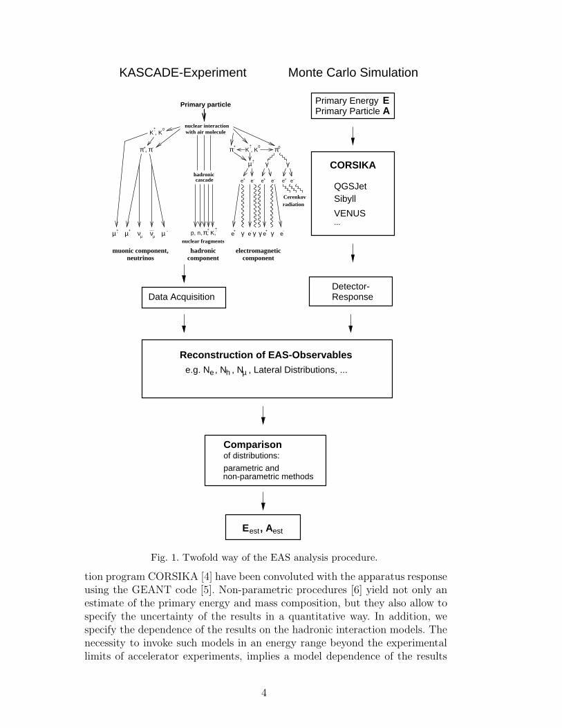
The analysis of the EAS variables to deduce the properties of the primaryparticle relies on the comparison with Monte Carlo simulations (MC) of theshower development (see Figure 1), including the detector response. Usuallyonly one or two EAS parameters are measured and various simplified proce-dures are used to describe the relation between the observed EAS propertiesand the nature and energy of the primary particle. The simplification often im-plies the use of parameterizations of the average behavior, which may bias theresults and limit the accuracy because fluctuations are neglected or not prop-erly accounted for. For the analysis of multivariate parameter distributionsand accounting for fluctuations more sophisticated methods are needed. Thedecades-old Bayesian methods and the neural network approaches, currentlyin vogue, meet these necessities. The methods facilitate an event-by-eventanalysis.
In the present paper we report on an investigation of the energy spectrum andmass composition of cosmic rays in the energy range of 1015−1016 eV, based onthe analysis of 700,000 EAS events. A subset of approximately 8000 showerswith cores near the center of the hadron calorimeter yields information on allthree components and has been studied in more detail. Following the analysisscheme shown in Figure 1, the simulated showers calculated with the simula-
3
neutrinosmuonic component,
componenthadronic
componentelectromagnetic
cascadehadronic
nuclear interactionwith air molecule
Cerenkovradiation
nuclear fragments
+-K , K0
+-K , K0+-π
e- e+ e+ e-
π0
+-µ
µ -νµνµµ+ +e
-e
+e
+-π+-, K,p, n,
e+ e-
-e
π , π+ -
µ+-
γ γ
γ γγ γ
Primary particle
CORSIKA
KASCADE-Experiment
Primary Particle APrimary Energy
ResponseDetector-
Data Acquisition
Comparison
parametric and
of distributions:
Reconstruction of EAS-Observables
E
E , A
e h
estest
...
Monte Carlo Simulation
QGSJetSibyll
VENUS
e.g. N , N , N , Lateral Distributions, ...µ
non-parametric methods
Fig. 1. Twofold way of the EAS analysis procedure.
tion program CORSIKA [4] have been convoluted with the apparatus responseusing the GEANT code [5]. Non-parametric procedures [6] yield not only anestimate of the primary energy and mass composition, but they also allow tospecify the uncertainty of the results in a quantitative way. In addition, wespecify the dependence of the results on the hadronic interaction models. Thenecessity to invoke such models in an energy range beyond the experimentallimits of accelerator experiments, implies a model dependence of the results
4
on the energy spectrum and mass composition. Quantifying this model de-pendence is one of the objectives of the present paper. The model dependenceis illustrated by using two different interaction models for the analysis. Thedependence implies not only the degree to which a particular EAS observableis correlated to energy and mass of the primary particle, it shows also howsensitively different EAS observables reveal primary mass. As an example, themass composition depends on the particular set of observables being consid-ered simultaneously in the analysis if the model is inconsistent with the datain all internal correlations.
It should be stressed that the present study emphasizes the methodical aspectsof how to infer energy spectrum and mass composition of CR rather thanproviding a final answer. This would require improved statistical accuracyboth in experiment and simulation and, first of all, a reduction of systematicuncertainties due to the incomplete knowledge of high energy interactions.Nevertheless our findings on spectrum and mass composition are compatiblewithin the methodical accuracy to the results of other experiments.
2 The KASCADE experiment
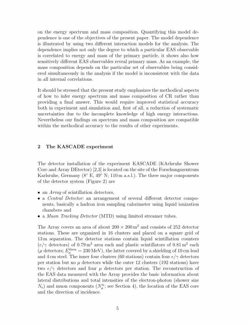
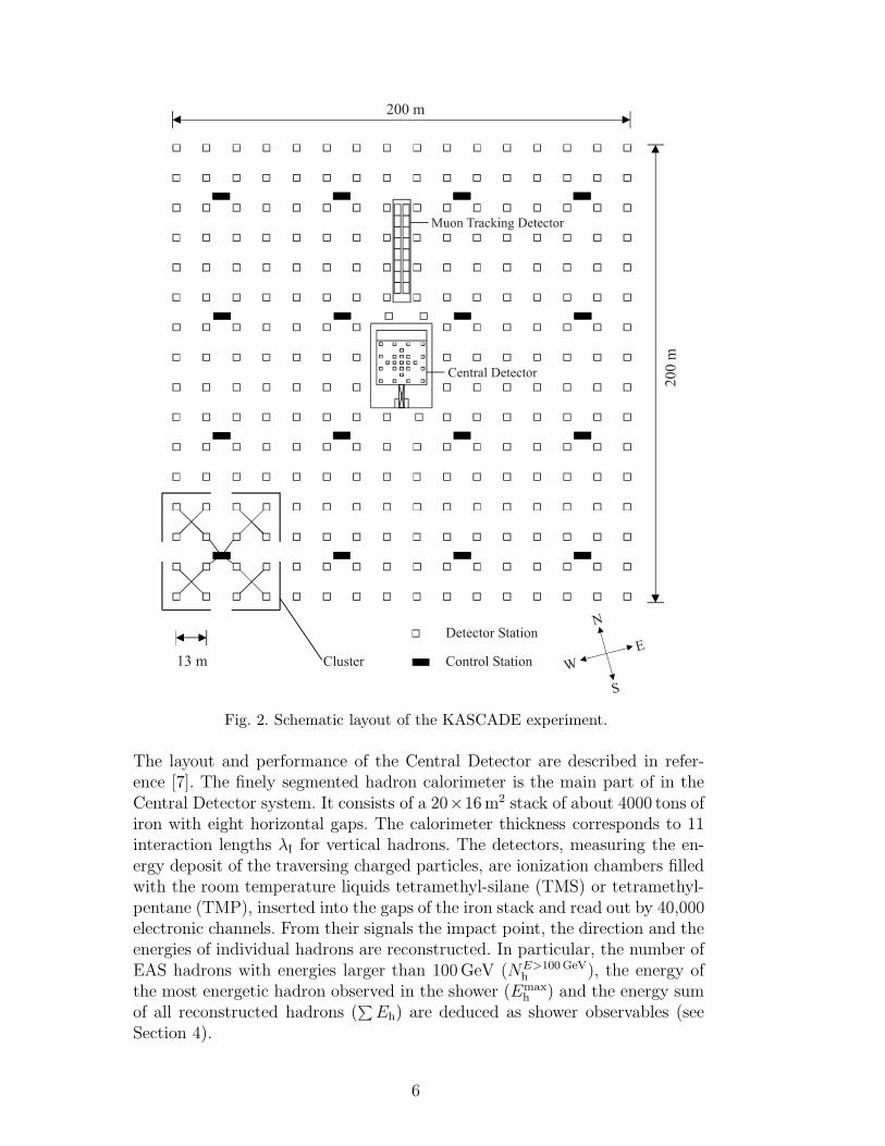
The detector installation of the experiment KASCADE (KArlsruhe ShowerCore and Array DEtector) [2,3] is located on the site of the ForschungszentrumKarlsruhe, Germany (8◦ E, 49◦ N; 110m a.s.l.). The three major componentsof the detector system (Figure 2) are
• an Array of scintillation detectors,• a Central Detector: an arrangement of several different detector compo-nents, basically a hadron iron sampling calorimeter using liquid ionizationchambers and
• a Muon Tracking Detector (MTD) using limited streamer tubes.
The Array covers an area of about 200× 200m2 and consists of 252 detectorstations. These are organized in 16 clusters and placed on a square grid of13m separation. The detector stations contain liquid scintillation counters(e/γ detectors) of 0.79m2 area each and plastic scintillators of 0.81m2 each(µ detectors; Ethres
µ = 230MeV), the latter covered by a shielding of 10 cm leadand 4 cm steel. The inner four clusters (60 stations) contain four e/γ detectorsper station but no µ detectors while the outer 12 clusters (192 stations) havetwo e/γ detectors and four µ detectors per station. The reconstruction ofthe EAS data measured with the Array provides the basic information aboutlateral distributions and total intensities of the electron-photon (shower sizeNe) and muon components (N tr
µ ; see Section 4), the location of the EAS coreand the direction of incidence.
5
Cluster13 m2
00
m
200 m
Detector Station
Central Detector
Muon Tracking Detector
Control Station
N
S
E
W
Fig. 2. Schematic layout of the KASCADE experiment.
The layout and performance of the Central Detector are described in refer-ence [7]. The finely segmented hadron calorimeter is the main part of in theCentral Detector system. It consists of a 20×16m2 stack of about 4000 tons ofiron with eight horizontal gaps. The calorimeter thickness corresponds to 11interaction lengths λI for vertical hadrons. The detectors, measuring the en-ergy deposit of the traversing charged particles, are ionization chambers filledwith the room temperature liquids tetramethyl-silane (TMS) or tetramethyl-pentane (TMP), inserted into the gaps of the iron stack and read out by 40,000electronic channels. From their signals the impact point, the direction and theenergies of individual hadrons are reconstructed. In particular, the number ofEAS hadrons with energies larger than 100GeV (NE>100GeV
h ), the energy ofthe most energetic hadron observed in the shower (Emax
h ) and the energy sumof all reconstructed hadrons (
∑
Eh) are deduced as shower observables (seeSection 4).
6
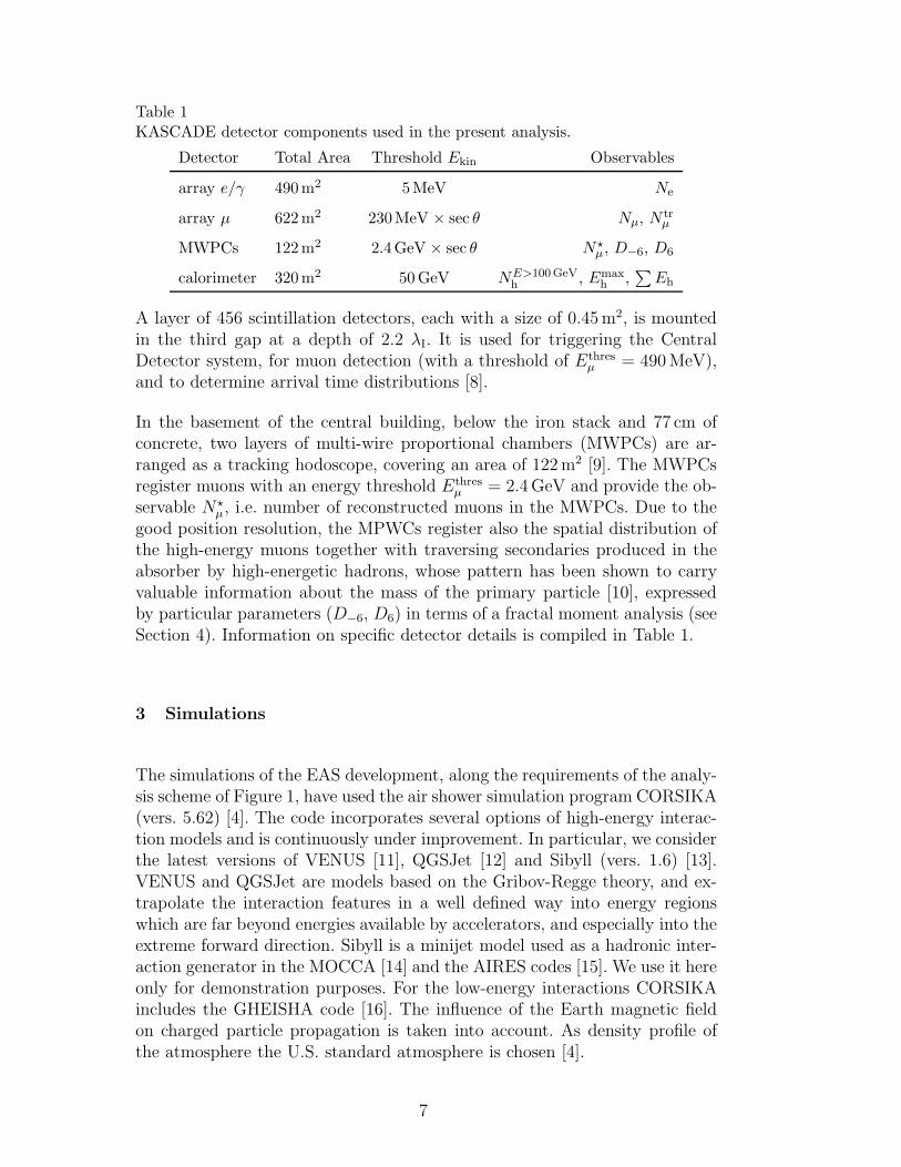
Table 1KASCADE detector components used in the present analysis.
Detector Total Area Threshold Ekin Observables
array e/γ 490m2 5MeV Ne
array µ 622m2 230MeV × sec θ Nµ, Ntrµ
MWPCs 122m2 2.4GeV × sec θ N⋆µ , D−6, D6
calorimeter 320m2 50GeV NE>100GeVh , Emax
h ,∑
Eh
A layer of 456 scintillation detectors, each with a size of 0.45m2, is mountedin the third gap at a depth of 2.2 λI. It is used for triggering the CentralDetector system, for muon detection (with a threshold of Ethres
µ = 490MeV),and to determine arrival time distributions [8].
In the basement of the central building, below the iron stack and 77 cm ofconcrete, two layers of multi-wire proportional chambers (MWPCs) are ar-ranged as a tracking hodoscope, covering an area of 122m2 [9]. The MWPCsregister muons with an energy threshold Ethres
µ = 2.4GeV and provide the ob-servable N⋆
µ, i.e. number of reconstructed muons in the MWPCs. Due to thegood position resolution, the MPWCs register also the spatial distribution ofthe high-energy muons together with traversing secondaries produced in theabsorber by high-energetic hadrons, whose pattern has been shown to carryvaluable information about the mass of the primary particle [10], expressedby particular parameters (D−6, D6) in terms of a fractal moment analysis (seeSection 4). Information on specific detector details is compiled in Table 1.
3 Simulations
The simulations of the EAS development, along the requirements of the analy-sis scheme of Figure 1, have used the air shower simulation program CORSIKA(vers. 5.62) [4]. The code incorporates several options of high-energy interac-tion models and is continuously under improvement. In particular, we considerthe latest versions of VENUS [11], QGSJet [12] and Sibyll (vers. 1.6) [13].VENUS and QGSJet are models based on the Gribov-Regge theory, and ex-trapolate the interaction features in a well defined way into energy regionswhich are far beyond energies available by accelerators, and especially into theextreme forward direction. Sibyll is a minijet model used as a hadronic inter-action generator in the MOCCA [14] and the AIRES codes [15]. We use it hereonly for demonstration purposes. For the low-energy interactions CORSIKAincludes the GHEISHA code [16]. The influence of the Earth magnetic fieldon charged particle propagation is taken into account. As density profile ofthe atmosphere the U.S. standard atmosphere is chosen [4].
7
Samples of at least 2000 proton and iron-induced showers have been simulatedwith all three models. Additionally for VENUS and QGSJet the intermediatemass primaries He, O and Si have been simulated. The energy distributionfollows a weighted power law with a spectral index of −2.7 in the energyrange of 1014 eV to 3.16·1016 eV, calculated in eight intervals. The zenith anglesare distributed in the range [13◦, 22◦]. The centers of the showers are spreaduniformly over an area which exceeds the surface of the hadron calorimeter by2m on each side. In addition, roughly the same number of simulated eventswith the centers of the showers within the Array are used. The signals observedin individual detectors are determined by tracking all secondary particles downto observation level and passing them through a detector response simulationprogram based on the GEANT package [5].
4 Event reconstruction and selection
The reconstruction of the EAS observables which is described in detail inpreceding publications of the KASCADE collaboration [10,17–20], applies aniterative procedure for reconstructing the shower size parameters. In a firststep the shower core location is determined by a center-of-gravity techniquefrom the energy deposit signals of all e/γ counters, and the shower directionis estimated by a simple plane fit using the timing information of the Arraydetectors. In addition, as rough first approximations, the electron size Ne andmuon size Nµ are estimated from summation of detector signals, taking intoaccount the actual shower core position on the grid. These parameter valuesare initial values for the further reconstruction steps. In the second step theshower direction is determined by fitting a conical shape of the shower disc tothe arrival times of the charged particle component, registered with the e/γcounters. The lateral distributions and their shape parameters are estimated,and N tr
µ and Ne are determined.
The muon size N trµ is the muon content within a range of distances from
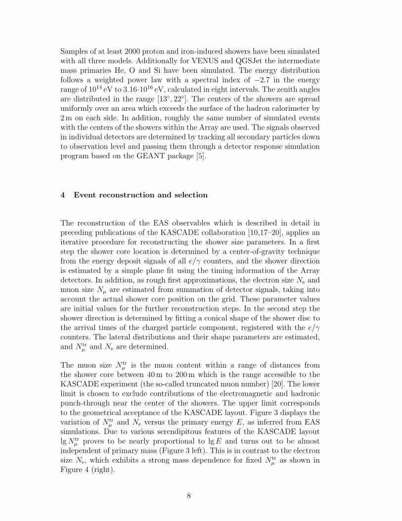
the shower core between 40m to 200m which is the range accessible to theKASCADE experiment (the so-called truncated muon number) [20]. The lowerlimit is chosen to exclude contributions of the electromagnetic and hadronicpunch-through near the center of the showers. The upper limit correspondsto the geometrical acceptance of the KASCADE layout. Figure 3 displays thevariation of N tr
µ and Ne versus the primary energy E, as inferred from EASsimulations. Due to various serendipitous features of the KASCADE layoutlgN tr
µ proves to be nearly proportional to lgE and turns out to be almostindependent of primary mass (Figure 3 left). This is in contrast to the electronsize Ne, which exhibits a strong mass dependence for fixed N tr
µ as shown inFigure 4 (right).
8
QGSJetp
Fe
VENUSp
Fe
Sibyllp
Fe
lg (E/GeV)
⟨Nµtr⟩
QGSJet
pFe
VENUS
pFe
Sibyll
p
Fe
lg (E/GeV)
⟨Ne⟩
10 3
10 4
10 5
5 5.5 6 6.5 7 7.5
10 4
10 5
10 6
5 5.5 6 6.5 7 7.5
Fig. 3. The mean values of the truncated muon number N trµ and electron number
Ne vs. primary energy as inferred on basis of the indicated interaction models. Forsake of clarity only QGSJet predictions are fitted by a linear function in lg-lg scale,in order to emphasize the much more pronounced mass dependence of the showersize Ne.
Contributions to the detector signals of other particles than electrons andmuons are eliminated by applying a lateral energy correction function to ap-propriate particle densities, which are fitted with a likelihood function to theNishimura Kamata Greisen (NKG) formula [21,22]. Values of the radius pa-rameters of 89m and 420m for electrons and muons, respectively, are used [17].For showers whose cores are located within 91m from the Array center 6 , thereconstruction uncertainty is about 2m for the location of the shower center,0.5◦ for the angle of incidence, and less than 10% and 20% for Ne and N tr
µ
values, respectively, at primary energies larger than 1015 eV.
Muon tracks observed with the MWPCs, reconstructed from pairs of hits inthe two MWPC layers (vertically separated by 38 cm [10]), are summed up toobtain N⋆
µ. A limit for the reconstructed angle of ±15◦ in zenith and ±45◦ inazimuth with respect to the shower axis determined from the Array is imposed(the azimuth cut is not applied for showers with zenith angles of < 10◦). Theanalysis of the number and spatial distribution of the muons and of producedsecondaries in terms of two generalized multi-fractal dimensions D−6 and D6
is discussed in [10]. These parameters characterize the spatial distributionof muons and high-energy (punch-through) hadrons as well as the degree offluctuations of particles in the shower core.
The reconstruction of the hadronic shower variables applies appropriate pat-tern recognition algorithms [18,19]. Energy clusters found in different detector
6 This number 91m results from the extension and the grid spacing of the detectorarray.
9
QGSJetp
Fe
VENUSp
Fe
Sibyllp
Fe
KASCADE
lg Nµtr
⟨Ne⟩
SibyllpFe
VENUSpFe
QGSJetpFe
KASCADE
lg Nµtr
⟨NhE
>100
GeV
⟩
10 4
10 5
10 6
3.5 4 4.5
10
10 2
3.75 4 4.25 4.5
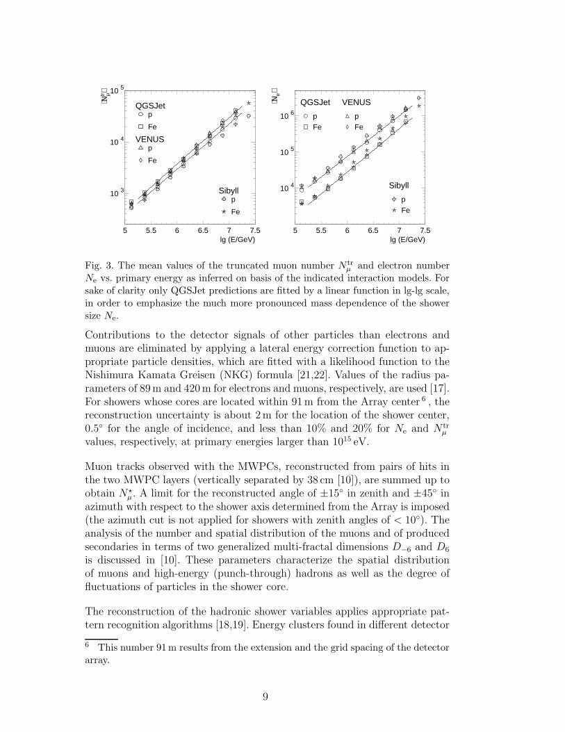
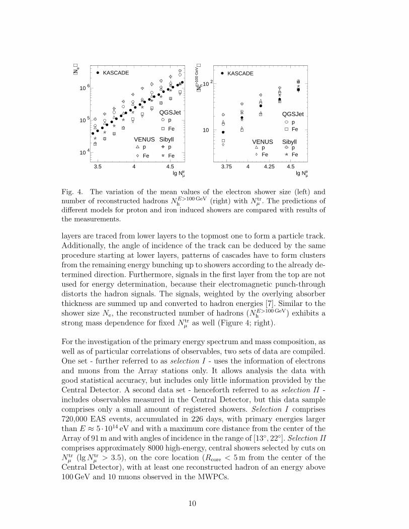
Fig. 4. The variation of the mean values of the electron shower size (left) andnumber of reconstructed hadrons NE>100GeV
h (right) with N trµ . The predictions of
different models for proton and iron induced showers are compared with results ofthe measurements.
layers are traced from lower layers to the topmost one to form a particle track.Additionally, the angle of incidence of the track can be deduced by the sameprocedure starting at lower layers, patterns of cascades have to form clustersfrom the remaining energy bunching up to showers according to the already de-termined direction. Furthermore, signals in the first layer from the top are notused for energy determination, because their electromagnetic punch-throughdistorts the hadron signals. The signals, weighted by the overlying absorberthickness are summed up and converted to hadron energies [7]. Similar to theshower size Ne, the reconstructed number of hadrons (NE>100GeV
h ) exhibits astrong mass dependence for fixed N tr
µ as well (Figure 4; right).
For the investigation of the primary energy spectrum and mass composition, aswell as of particular correlations of observables, two sets of data are compiled.One set - further referred to as selection I - uses the information of electronsand muons from the Array stations only. It allows analysis the data withgood statistical accuracy, but includes only little information provided by theCentral Detector. A second data set - henceforth referred to as selection II -includes observables measured in the Central Detector, but this data samplecomprises only a small amount of registered showers. Selection I comprises720,000 EAS events, accumulated in 226 days, with primary energies largerthan E ≈ 5 ·1014 eV and with a maximum core distance from the center of theArray of 91m and with angles of incidence in the range of [13◦, 22◦]. Selection II
comprises approximately 8000 high-energy, central showers selected by cuts onN tr
µ (lgN trµ > 3.5), on the core location (Rcore < 5m from the center of the
Central Detector), with at least one reconstructed hadron of an energy above100GeV and 10 muons observed in the MWPCs.
10
5 Non-parametric analyses
The present analysis of mass composition and energy spectrum avoids thebias inherent in parametric procedures and is performed for individual eventsby use of multivariate non-parametric Bayesian and neural network decisionmethods. In this way we are able to specify, in a transparent and coherent way,how conclusive and trustworthy our results are, as expressed by true classifi-cation and misclassification matrices of the results. A brief outline and moredetails of the applied methods are given in Appendix A and in reference [23].
The combination of the total muon content Nµ and the shower size Ne hasbeen shown to be sensitive to primary mass and is applied in numerous exper-imental studies, using suitable parameterizations of the predicted lgNµ/ lgNe
relation with the primary mass. However, as indicated above, the total muoncontent Nµ, although displaying some dependence on primary mass, is a quan-tity not easily accessible experimentally without additional assumptions aboutthe shape of the lateral muon density distribution at large distances from theshower core. Therefore, we prefer to consider the truncated muon number N tr
µ ,which - on average - proves to be nearly independent from primary mass (seeFigure 3), but it is, on the other hand, a rather sensitive energy identifier.Thus, at fixed N tr
µ , the information about the mass is essentially provided bythe shower size Ne [20]. In cases of other EAS observables mass and energysensitivities are, in general, less well marked, and in principle, each shower vari-able carries information simultaneously on mass and energy in a way which isadditionally affected by the considerable fluctuations of the shower develop-ment. The most sensitive EAS observables, Ne and N tr
µ , display the smallestintrinsic and sampling fluctuations.
5.1 Mass composition
Due to the limited number of simulated EAS and the correspondingly limitedstatistical accuracy it is hardly reasonable to use the full set of observablessimultaneously to achieve a reliable result about mass composition (curse ofdimensionality condition; see Appendix A). Hence we consider simultaneouslyonly a few observables.
Each simulated or measured event is represented by an observation vectorx = (Ne, N
trµ , . . .) of the n observables. Applying the technique described in
Appendix A the likelihood (probability density distribution) p(x|ωi) of anevent for each class ωi ∈ {p,O,Fe} can be calculated, i.e. the probability ofan event x belonging to a given class ωi.
As an example, the superposition of the estimated probability density distri-
11
3.63.7
3.83.9
44.1
4.24.3
4.44.5
5
5.2
5.4
5.6
5.8
60
0.050.1
0.15
p(x|
ωi)
lg N µ
tr lg Ne
p O Fe
3.53.6
3.73.8
3.94
4.14.2
4.34.4
4.5
1.51.6
1.71.8
1.92
2.12.2
2.32.4
0.05
0.1
0.15
p(x|
ωi)
lg
N µtr lg N ✶
µ
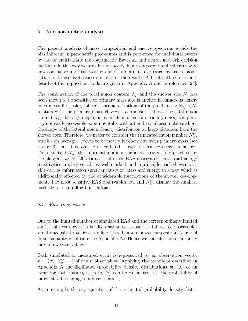
Fig. 5. Superposition of three probability density distributions∑3
i=1 p(x|ωi)/3 de-duced from QGSJet simulations using the observables Ne and N tr
µ (left) as well asN⋆
µ and N trµ (right). Events in the dark shaded area mark the region classified as
iron, middle grey as oxygen, and light grey as proton (selection II).
butions, referring to two sets of different observables, are displayed in Fig-ure 5 (based on QGSJet simulations). The regions where p(x|ωp), p(x|ωO) andp(x|ωFe) are larger than the other two possibilities are colored light, middleand dark grey, respectively. The left graph shows the density distribution cal-culated in the two dimensional space of the observables Ne and N tr
µ . A roughseparation can be recognized, but also a strong overlapping of the likelihooddistributions has to be admitted.
The right-hand graph of Figure 5 shows an example of two observables (N⋆µ
and N trµ ), which exhibit only weak mass-discrimination power. Correspond-
ingly, the density distributions of the three particle types are intermixed, andreliable conclusions could not be drawn. In case of selection II the mass compo-sition is reconstructed for different sets of observables using the Bayes theorem(Equation A.1). When the estimated posterior probability p(ωi|x) is largerthan p(ωj|x), then the event is assigned to class ωi, otherwise to class ωj .Taking into account (by Equation A.1) the estimated number of incorrectlyclassified events (i.e. misclassification rates) (Table 2) the true proportions ofthe different particle types are reconstructed.
The classification rates Pij = Pωi→ωj(see Appendix: Equation A.1 and Fig-
ure A.1) give the fraction of correctly, Pii, and wrongly, Pij, classified eventswith i 6= j, an example for three mass class is given in Table 2. Of course,the sum of each row has to be 100%. In the most probable cases the differentparticle types are identified correctly, but the knowledge of the incorrectlyclassified events could be used for a correction due to the mis-classification.In addition, the rates for the intermediate mass particle types, He and Si,are given. Helium is mostly classified as protons (57%) and silicon as oxygen(54%). Due to the stronger fluctuations and weaker correlations with mass
12
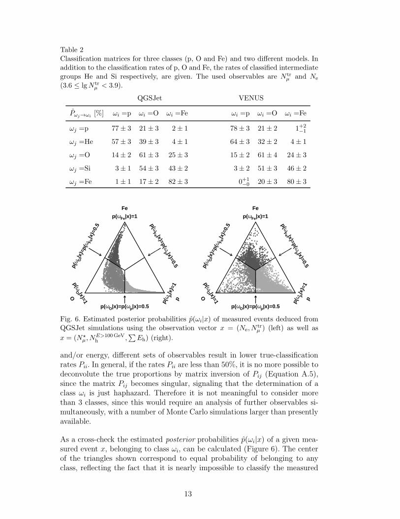
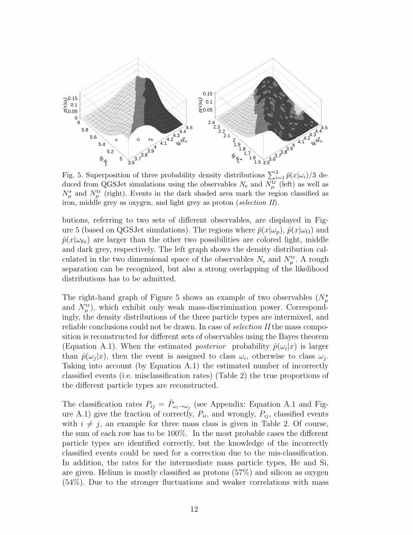
Table 2Classification matrices for three classes (p, O and Fe) and two different models. Inaddition to the classification rates of p, O and Fe, the rates of classified intermediategroups He and Si respectively, are given. The used observables are N tr
µ and Ne
(3.6 ≤ lgN trµ < 3.9).
QGSJet VENUS
Pωj→ωi[%] ωi =p ωi =O ωi =Fe ωi =p ωi =O ωi =Fe
ωj =p 77± 3 21± 3 2± 1 78± 3 21± 2 1+2−1
ωj =He 57± 3 39± 3 4± 1 64± 3 32± 2 4± 1
ωj =O 14± 2 61± 3 25± 3 15± 2 61± 4 24± 3
ωj =Si 3± 1 54± 3 43± 2 3± 2 51± 3 46± 2
ωj =Fe 1± 1 17± 2 82± 3 0+1−0 20± 3 80± 3
p(ωO|x)=p(ωp|x)=0.5
p(ωFe |x)=p(ω
p |x)=0.5p(ω O
|x)=
p(ω Fe
|x)=
0.5
p(ω p
|x)=
1p
p(ωO |x)=1
O
p(ωFe|x)=1
Fe
p(ωO|x)=p(ωp|x)=0.5
p(ωFe |x)=p(ω
p |x)=0.5p(ω O
|x)=
p(ω Fe
|x)=
0.5
p(ω p
|x)=
1p
p(ωO |x)=1
O
p(ωFe|x)=1
Fe
Fig. 6. Estimated posterior probabilities p(ωi|x) of measured events deduced fromQGSJet simulations using the observation vector x = (Ne, N
trµ ) (left) as well as
x = (N⋆µ , N
E>100GeVh ,
∑
Eh) (right).
and/or energy, different sets of observables result in lower true-classificationrates Pii. In general, if the rates Pii are less than 50%, it is no more possible todeconvolute the true proportions by matrix inversion of Pij (Equation A.5),since the matrix Pij becomes singular, signaling that the determination of aclass ωi is just haphazard. Therefore it is not meaningful to consider morethan 3 classes, since this would require an analysis of further observables si-multaneously, with a number of Monte Carlo simulations larger than presentlyavailable.
As a cross-check the estimated posterior probabilities p(ωi|x) of a given mea-sured event x, belonging to class ωi, can be calculated (Figure 6). The centerof the triangles shown correspond to equal probability of belonging to anyclass, reflecting the fact that it is nearly impossible to classify the measured
13
lg Nµtr
Rel
ativ
e A
bund
ance
QGSJetpOFe
VENUSpOFe
lg Nµtr
⟨ln A
⟩
QGSJet
VENUS
0
0.1
0.2
0.3
0.4
0.5
0.6
0.7
0.8
0.9
1
3.6 3.8 4 4.2 4.40
0.5
1
1.5
2
2.5
3
3.5
3.6 3.8 4 4.2 4.4
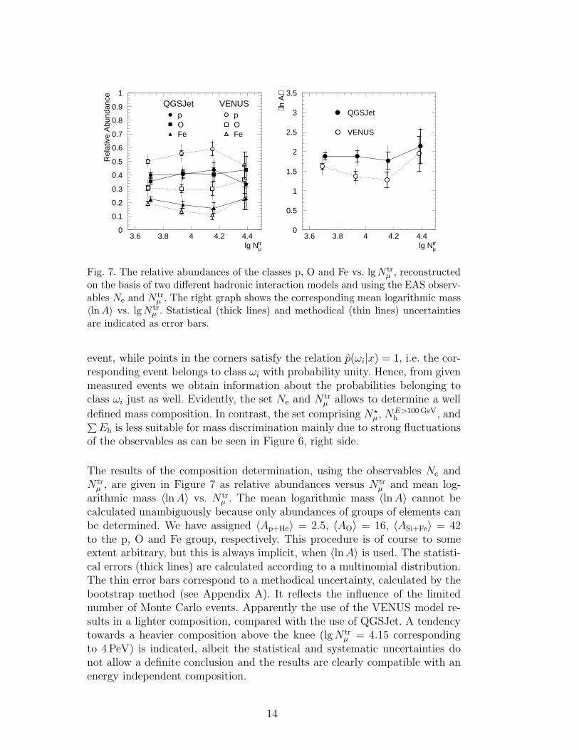
Fig. 7. The relative abundances of the classes p, O and Fe vs. lgN trµ , reconstructed
on the basis of two different hadronic interaction models and using the EAS observ-ables Ne and N tr
µ . The right graph shows the corresponding mean logarithmic mass〈lnA〉 vs. lgN tr
µ . Statistical (thick lines) and methodical (thin lines) uncertaintiesare indicated as error bars.
event, while points in the corners satisfy the relation p(ωi|x) = 1, i.e. the cor-responding event belongs to class ωi with probability unity. Hence, from givenmeasured events we obtain information about the probabilities belonging toclass ωi just as well. Evidently, the set Ne and N tr
µ allows to determine a well
defined mass composition. In contrast, the set comprising N⋆µ, N
E>100GeVh , and
∑
Eh is less suitable for mass discrimination mainly due to strong fluctuationsof the observables as can be seen in Figure 6, right side.
The results of the composition determination, using the observables Ne andN tr
µ , are given in Figure 7 as relative abundances versus N trµ and mean log-
arithmic mass 〈lnA〉 vs. N trµ . The mean logarithmic mass 〈lnA〉 cannot be
calculated unambiguously because only abundances of groups of elements canbe determined. We have assigned 〈Ap+He〉 = 2.5, 〈AO〉 = 16, 〈ASi+Fe〉 = 42to the p, O and Fe group, respectively. This procedure is of course to someextent arbitrary, but this is always implicit, when 〈lnA〉 is used. The statisti-cal errors (thick lines) are calculated according to a multinomial distribution.The thin error bars correspond to a methodical uncertainty, calculated by thebootstrap method (see Appendix A). It reflects the influence of the limitednumber of Monte Carlo events. Apparently the use of the VENUS model re-sults in a lighter composition, compared with the use of QGSJet. A tendencytowards a heavier composition above the knee (lgN tr
µ = 4.15 correspondingto 4 PeV) is indicated, albeit the statistical and systematic uncertainties donot allow a definite conclusion and the results are clearly compatible with anenergy independent composition.
14
lg Nµtr
⟨ln A
⟩Ne, Nµ
tr, N✶µ, Nh
E>100 GeV, ΣEh
Ne, Nµtr, Nh
E>100 GeV
Ne, Nµtr, N✶
µ
Ne, N✶µ
average value
lg Nµtr
⟨ln A
⟩
Nµtr,Nh
E>100 GeV,ΣEh,Ehmax
Nµtr,N✶
µ,NhE>100 GeV
Nµtr,N✶
µ,NhE>100 GeV,ΣEh
Nµtr,ΣEh,D-6
average value
0.5
1
1.5
2
2.5
3
3.5
3.6 3.8 4 4.2 4.40.5
1
1.5
2
2.5
3
3.5
3.6 3.8 4 4.2 4.4
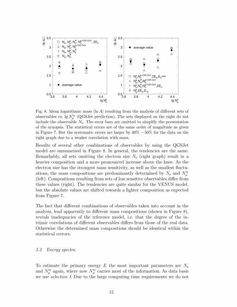
Fig. 8. Mean logarithmic mass 〈lnA〉 resulting from the analysis of different sets ofobservables vs. lgN tr
µ (QGSJet prediction). The sets displayed on the right do notinclude the observable Ne. The error bars are omitted to simplify the presentationof the synopsis. The statistical errors are of the same order of magnitude as givenin Figure 7. But the systematic errors are larger by 40%− 50% for the data on theright graph due to a weaker correlation with mass.
Results of several other combinations of observables by using the QGSJetmodel are summarized in Figure 8. In general, the tendencies are the same.Remarkably, all sets omitting the electron size Ne (right graph) result in aheavier composition and a more pronounced increase above the knee. As theelectron size has the strongest mass sensitivity, as well as the smallest fluctu-ations, the mass compositions are predominantly determined by Ne and N tr
µ
(left). Compositions resulting from sets of less sensitive observables differ fromthese values (right). The tendencies are quite similar for the VENUS model,but the absolute values are shifted towards a lighter composition as expectedfrom Figure 7.
The fact that different combinations of observables taken into account in theanalysis, lead apparently to different mass compositions (shown in Figure 8),reveals inadequacies of the reference model, i.e. that the degree of the in-trinsic correlations of different observables differs from those of the real data.Otherwise the determined mass compositions should be identical within thestatistical errrors.
5.2 Energy spectra
To estimate the primary energy E the most important parameters are Ne
and N trµ again, where now N tr
µ carries most of the information. As data basiswe use selection I. Due to the large computing time requirements we do not
15
lg(E/GeV)
∆E/E p
OFe
lg(E/GeV)
∆E/E p
OFe
-1
-0.8
-0.6
-0.4
-0.2
0
0.2
0.4
0.6
0.8
1
6 6.5 7-1
-0.8
-0.6
-0.4
-0.2
0
0.2
0.4
0.6
0.8
1
6 6.5 7
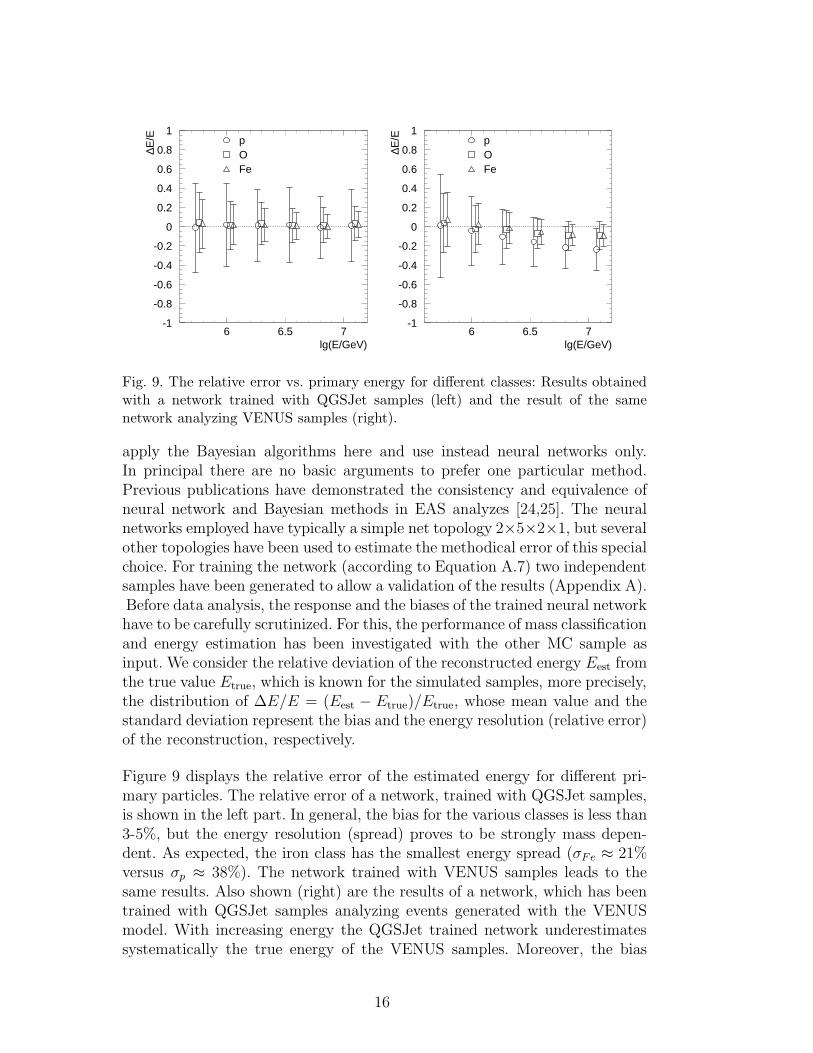
Fig. 9. The relative error vs. primary energy for different classes: Results obtainedwith a network trained with QGSJet samples (left) and the result of the samenetwork analyzing VENUS samples (right).
apply the Bayesian algorithms here and use instead neural networks only.In principal there are no basic arguments to prefer one particular method.Previous publications have demonstrated the consistency and equivalence ofneural network and Bayesian methods in EAS analyzes [24,25]. The neuralnetworks employed have typically a simple net topology 2×5×2×1, but severalother topologies have been used to estimate the methodical error of this specialchoice. For training the network (according to Equation A.7) two independentsamples have been generated to allow a validation of the results (Appendix A).Before data analysis, the response and the biases of the trained neural networkhave to be carefully scrutinized. For this, the performance of mass classificationand energy estimation has been investigated with the other MC sample asinput. We consider the relative deviation of the reconstructed energy Eest fromthe true value Etrue, which is known for the simulated samples, more precisely,the distribution of ∆E/E = (Eest − Etrue)/Etrue, whose mean value and thestandard deviation represent the bias and the energy resolution (relative error)of the reconstruction, respectively.
Figure 9 displays the relative error of the estimated energy for different pri-mary particles. The relative error of a network, trained with QGSJet samples,is shown in the left part. In general, the bias for the various classes is less than3-5%, but the energy resolution (spread) proves to be strongly mass depen-dent. As expected, the iron class has the smallest energy spread (σFe ≈ 21%versus σp ≈ 38%). The network trained with VENUS samples leads to thesame results. Also shown (right) are the results of a network, which has beentrained with QGSJet samples analyzing events generated with the VENUSmodel. With increasing energy the QGSJet trained network underestimatessystematically the true energy of the VENUS samples. Moreover, the bias
16
Energymodel lg(E/GeV)
I(E
) ×
E2.
75
[m-2
s-1
sr-1
GeV
1.75
]
QGSJetQGSJet
VENUSVENUS
EnergyQGSJet lg(E/GeV)
(∆E
/E) m
odel
10 4
10 5
6 6.2 6.4 6.6 6.8 7 7.2
-0.5-0.4-0.3-0.2-0.1
00.10.20.30.40.5
6 6.5 7
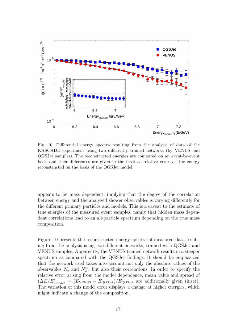
Fig. 10. Differential energy spectra resulting from the analysis of data of theKASCADE experiment using two differently trained networks (by VENUS andQGSJet samples). The reconstructed energies are compared on an event-by-eventbasis and their differences are given in the inset as relative error vs. the energyreconstructed on the basis of the QGSJet model.
appears to be mass dependent, implying that the degree of the correlationbetween energy and the analyzed shower observables is varying differently forthe different primary particles and models. This is a caveat to the estimate oftrue energies of the measured event samples, namly that hidden mass depen-dent correlations lead to an all-particle spectrum depending on the true masscomposition.
Figure 10 presents the reconstructed energy spectra of measured data result-ing from the analysis using two different networks, trained with QGSJet andVENUS samples. Apparently, the VENUS trained network results in a steeperspectrum as compared with the QGSJet findings. It should be emphasizedthat the network used takes into account not only the absolute values of theobservables Ne and N tr
µ , but also their correlations. In order to specify therelative error arising from the model dependence, mean value and spread of(∆E/E)model = (EVENUS − EQGSJet)/EQGSJet are additionally given (inset).The variation of this model error displays a change at higher energies, whichmight indicate a change of the composition.
17
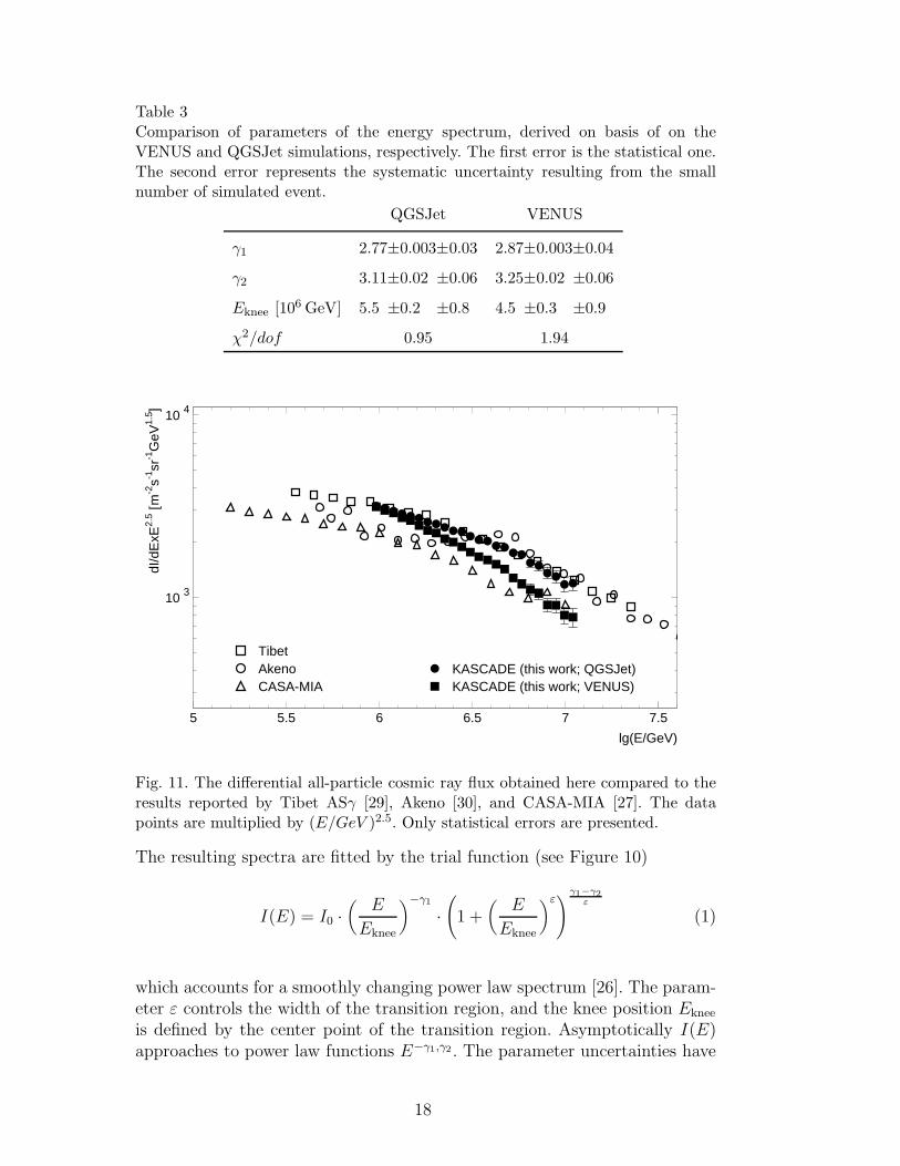
Table 3Comparison of parameters of the energy spectrum, derived on basis of on theVENUS and QGSJet simulations, respectively. The first error is the statistical one.The second error represents the systematic uncertainty resulting from the smallnumber of simulated event.
QGSJet VENUS
γ1 2.77±0.003±0.03 2.87±0.003±0.04
γ2 3.11±0.02 ±0.06 3.25±0.02 ±0.06
Eknee [106 GeV] 5.5 ±0.2 ±0.8 4.5 ±0.3 ±0.9
χ2/dof 0.95 1.94
10 3
10 4
5 5.5 6 6.5 7 7.5
KASCADE (this work; VENUS)KASCADE (this work; QGSJet)
lg(E/GeV)
dI/d
ExE
2.5 [m
-2s-1
sr-1
GeV
1.5 ]
AkenoTibet
CASA-MIA
Fig. 11. The differential all-particle cosmic ray flux obtained here compared to theresults reported by Tibet ASγ [29], Akeno [30], and CASA-MIA [27]. The datapoints are multiplied by (E/GeV )2.5. Only statistical errors are presented.
The resulting spectra are fitted by the trial function (see Figure 10)
I(E) = I0 ·(
E
Eknee
)−γ1
·(
1 +(
E
Eknee
)ε)
γ1−γ2ε
(1)
which accounts for a smoothly changing power law spectrum [26]. The param-eter ε controls the width of the transition region, and the knee position Eknee
is defined by the center point of the transition region. Asymptotically I(E)approaches to power law functions E−γ1,γ2 . The parameter uncertainties have
18
been studied by calculating the errors I(E)±∆I(E) using the sampling cor-relation matrix. But the resulting error bands are so narrow that it does notvisibly differ from the I(E)-line. The best-fit results are given in Table 3, in-cluding statistical errors as well as the methodical error derived from differenttraining parameters of the neural network. It is obvious that the statistical er-rors are considerably smaller than the systematic uncertainties resulting fromthe small number of simulated events and from interaction models.
Figure 11 compares the spectra of Figure 10 with results reported by otherexperiments. All measurements, independently from each other, show a steep-ening above a particular energy: the knee. But the absolute intensity of theflux and the position of the knee obviously differ. This is most likely due todifferent model assumptions or energy conversion functions used. The consid-erable deviation between CASA-MIA [27] and the other two experiments maybe explained in this way. CASA-MIA used the Sibyll model for constructingan energy estimator E = f(Ne, Nµ) from the electron and muon sizes. Thefact that Sybill predicts significantly lower values of Nµ and larger values forNe [28] as compared to QGSJet and VENUS, could lead to a systematic shiftof the spectrum towards lower energies. In view of the considerable modeldependence of our results, the overlap with some of the other experimentsshould not be taken as evidence for or against any of them.
5.3 Combined analysis of energy and mass
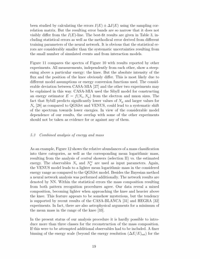
As an example, Figure 12 shows the relative abundances of a mass classificationinto three categories, as well as the corresponding mean logarithmic mass,resulting from the analysis of central showers (selection II) vs. the estimatedenergy. The observables Ne and N tr
µ are used as input parameters. Again,the VENUS model leads to a lighter mean logarithmic mass in the consideredenergy range as compared to the QGSJet model. Besides the Bayesian methoda neural network analysis was performed additionally. The network results aredenoted by NN. Within the statistical errors the mass composition resultingfrom both pattern recognition procedures agree. Our data reveal a mixedcomposition, becoming lighter when approaching the knee and heavier abovethe knee. This feature appears to be somehow mysterious, but the tendencyis supported by recent results of the CASA-BLANCA [31] and HEGRA [32]experiments. In fact, there are also astrophysical arguments for a minimum ofthe mean mass in the range of the knee [33].
In the present status of our analysis procedure it is hardly possible to intro-duce more than three classes for the reconstruction of the mass composition.If this were to be attempted additional observables had to be included. A finerbinning of the energy scale (beyond the energy resolution (∆E/E)est) for the
19
lg(E/GeV)
Rel
ativ
e A
bund
ance
QGSJet
pOFe
lg(E/GeV)
⟨ln A
⟩
QGSJet
NNBayes
VENUS
NNBayes
0
0.1
0.2
0.3
0.4
0.5
0.6
0.7
0.8
0.9
1
6 6.25 6.5 6.75 71
1.25
1.5
1.75
2
2.25
2.5
2.75
3
3.25
3.5
6 6.25 6.5 6.75 7
Fig. 12. Relative abundances reconstructed by Bayes classification vs. the recon-structed energy based on the QGSJet model and using Ne and N tr
µ . Additionally,the corresponding mean logarithmic mass 〈lnA〉 (right; Bayes) and the correspond-ing variation resulting from the neural network analysis (NN) are given. The errorbars represent the statistical (thick) and methodical (thin) uncertainties.
spectra of single masses would require to deconvolute the resolution effects. Inthe actual analysis this step has not been performed and only a few represen-tative values of the varying mass composition (and no detailed energy spectraof the different mass classes) have been presented. To analyze the data beyondthis limit we need, in the simplest case, to construct from the misclassificationmatrices a matrix AAA′;EE′ deconvoluting mass and energy resolution effects.Stressing once more the curse of dimensionality (see Appendix A), a very largenumber of simulated events is required for the determination of such a matrix(at least 150000 simulated events are needed). For the same reasons we arepresently unable to infer any significant fine structure from the all-particleenergy spectrum beyond the resolution (∆E/E)est.
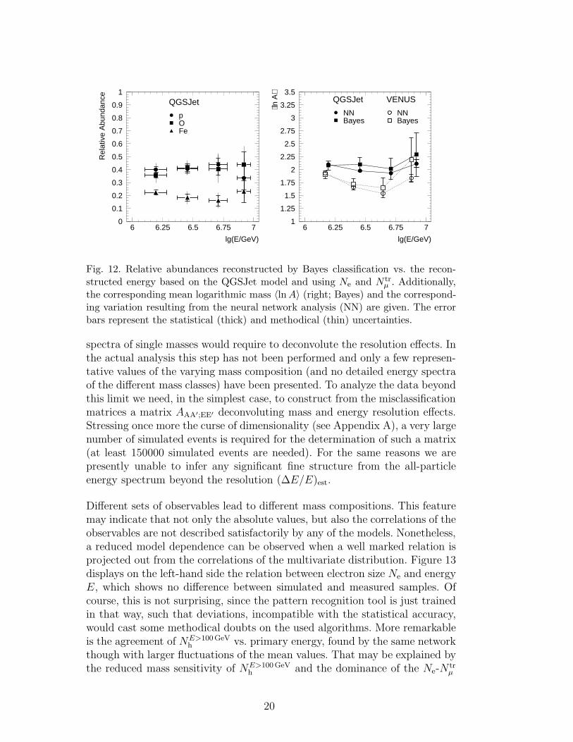
Different sets of observables lead to different mass compositions. This featuremay indicate that not only the absolute values, but also the correlations of theobservables are not described satisfactorily by any of the models. Nonetheless,a reduced model dependence can be observed when a well marked relation isprojected out from the correlations of the multivariate distribution. Figure 13displays on the left-hand side the relation between electron size Ne and energyE, which shows no difference between simulated and measured samples. Ofcourse, this is not surprising, since the pattern recognition tool is just trainedin that way, such that deviations, incompatible with the statistical accuracy,would cast some methodical doubts on the used algorithms. More remarkableis the agreement of NE>100GeV
h vs. primary energy, found by the same networkthough with larger fluctuations of the mean values. That may be explained bythe reduced mass sensitivity of NE>100GeV
h and the dominance of the Ne-Ntrµ
20
lg(E/GeV)
⟨Ne⟩
KASCADE
pOFe
QGSJet
pOFe
lg(E/GeV)
⟨NhE
>100
GeV
⟩
KASCADE
pOFe
QGSJet
pOFe
10 5
10 6
6 6.25 6.5 6.75 7
10
10 2
6 6.25 6.5 6.75 7
Fig. 13. The projected relations lgNe and lgNE>100GeVh , respectively, vs. lg(E/GeV)
from two neural networks, trained to estimate the energy and mass of the measuredevents using Ne and N tr
µ as EAS observables.
correlation (compare the observable sets in Figure 8 left). Nevertheless, withinthe statistical significance level (in terms of hypotheses tests like student t-test) no difference between data and model predictions can be stated.
6 Discussion and conclusion
The present paper aims at presenting methods of a determination of primaryenergy spectrum and mass composition of cosmic rays in the energy range1015 − 5 · 1016 eV by an event-by-event analysis of EAS data. The specific me-thodical feature is the use of a non-parametric approach, studying multivariatedistributions of a number of EAS observables [34,25].
The present approach to obtain information about the EAS primaries hasfollowing merits:
• It specifies the inevitable model dependence of any statement about spec-trum and mass composition, introduced through the patterns provided bythe Monte Carlo simulations on basis of a particular hadronic interactionmodel.
• The model dependence is not only revealed by the results from the analysisof single EAS observables when comparing different hadronic interactionmodels, but the approach specifies also the degree of correlations betweendifferent observables used for the multivariate analysis.
• This feature provides the possibility to test a specific hadronic interactionmodel by exploring the internal consistency of the results, when the outcome
21
of different sets of observables are considered. This aspect is of greatestimportance for approaching the best model reproducing the observations inthe most consistent way.
• Comparing the KASCADE findings with other experiments shows that thediscrepancies between results can well be attributed to the different inter-action models employed.
Acknowledgements
We acknowledge various clarifying discussions with Ralph Engel, Sergej Ostap-chenko and Klaus Werner about the use and embedding of the hadronic inter-action models Sibyll, QGSJet and VENUS in the Monte Carlo EAS simulationcode CORSIKA. The authors would like to thank the members of the engi-neering and technical staff of the KASCADE collaboration who contributedwith enthusiasm and engagement to the success of the experiment. The workhas been supported by the Ministry for Research of the Federal Government ofGermany, by a grant of the Romanian National Agency for Science, Researchand Technology, by a research grant (No. 94964) of the Armenian Govern-ment, and by the ISTC project A116. The collaborating group of the CosmicRay Division of the Soltan Institute of Nuclear Studies in Lodz and of theUniversity of Lodz is supported by the Polish State Committee for ScientificResearch. The KASCADE collaboration work is embedded in the frame ofscientific-technical cooperation (WTZ) projects between Germany and Roma-nia (No. RUM-014-97), Poland (No. POL 99/005) and Armenia (No. 002-98).
References
[1] G.V. Kulikov and G.B. Khristiansen, Soviet Physics JETP 35 (1959) 441.
[2] P. Doll et al., KfK-Report 4686, Kernforschungszentrum Karlsruhe 1990.
[3] H.O. Klages et al., Nucl. Phys. B (Proc. Suppl.) 52B (1997) 92.
[4] D. Heck et al., FZKA-Report 6019, Forschungszentrum Karlsruhe 1998.
[5] CERN Program Library Long Writeups W5013 1993.
[6] A.A. Chilingarian, Comput. Phys. Commun. 54 (1989) 381.
[7] J. Engler et al., Nucl. Inst. Meth. A 427 (1999) 528.
[8] T. Antoni et al., (KASCADE Collaboration), ”Time Structure of the EAS MuonComponent measured by the KASCADE Experiment”, Astropart. Phys., inpress.
22
[9] H. Bozdog et al., ”The detector system for measurement of multiple cosmicmuons in the central detector of KASCADE”, Nucl. Inst. Meth., submitted.
[10] A. Haungs et al., Nucl. Inst. Meth. A 372 (1996) 515.
[11] K. Werner, Phys. Rep. 232 (1993) 87.
[12] N.N. Kalmykov, S.S. Ostapchenko, Yad. Fiz. 56 (1993) 105.
[13] J. Engel et al., Phys. Rev. D 50 (1994) 5013.
[14] A.M. Hillas, Proc. 17th Int. Cosmic Ray Conference, Paris 8 (1981) 193.
[15] S. Sciutto, ”AIRES a System for Air Shower Simulations-Version 2.2.0”, AugerProject Report GAP-99-044, 1999.
[16] H. Fesefeldt, Report PITHA 85/02, RWTH Aachen, Germany 1985.
[17] T. Antoni et al., (KASCADE Collaboration), Astropart. Phys. 14 (2001) 245.
[18] J. Unger et al., Proc. 25th Int. Cosmic Ray Conference, Durban 6 (1997) 145;J. Unger, FZKA-Report 5896, Forschungszentrum Karlsruhe 1997, in German.
[19] J.R. Horandel, FZKA-Report 6015, Forschungszentrum Karlsruhe 1998, inGerman.
[20] J.H. Weber et al., Proc. 25th Int. Cosmic Ray Conference, Durban 6 (1997)153; J.H. Weber, FZKA-Report 6339, Forschungszentrum Karlsruhe 1999, inGerman.
[21] K. Greisen, Progress in Cosmic Ray Physics 3, North Holland Publ. 1956.
[22] K. Kamata, J. Nishimura, Prog. Theoret. Phys. Suppl. 6 (1958) 93.
[23] A.A. Chilingarian, ANI users guide, unpublished.
[24] M. Roth, FZKA-Report 6262, Forschungszentrum Karlsruhe 1999, in German.
[25] A.A. Chilingarian et al., Nucl. Phys. B (Proc. Suppl.) 52B (1997) 237.
[26] S.V. Ter-Antonyan, L.S. Haroyan, preprint hep-ex/0003006.
[27] M.A.K. Glasmacher et al., Astropart. Phys. 10 (1999) 291.
[28] T. Antoni et al., (KASCADE Collaboration), J. Phys. G: Nucl. Part. Phys. 25(1999) 2161.
[29] M. Amenomori et al., Astrophys. J. 461 (1996) 408.
[30] M. Nagano et al., J. Phys. G: Nucl. Phys. 10 (1984) 1295.
[31] J.W. Fowler et al., preprint astro-ph/0003190, submitted to Astropart. Phys.
[32] F. Arqueros et al., preprint astro-ph/9908202, submitted to Astron. Astrophys.
[33] S. Swordy, Proc. 24th Int. Cosmic Ray Conference, Rome 2 (1995) 697.
23
[34] A.A. Chilingarian, H.Z. Zazian, Pattern Recognition Letters V11 (1990) 781.
[35] C.M. Bishop, Neural Networks for Pattern Recognition, Oxford University Press1995.
[36] K. Fukunaka, Introduction to Statistical Pattern Recognition, Academic Press1972.
[37] E. Parzen, Annals of Mathematical Statistics 33 (1962) 1065.
[38] T. Cacoullos, Annals of the Institute of Statistical Mathematics, Tokyo (1966)179.
[39] T. Bayes, Phil. Trans. Roy. Soc. 53 (1763) 54 (reprinted in Biometrika 45
(1958) 296).
[40] D. Rummelhart, J. McClelland, Parallel Distributed Processing, MIT Press,Cambridge 1986.
24
A Non-parametric statistical inference
Pattern recognition techniques are efficient tools to determine the correct asso-ciation of a given sample to a certain category or class. From the measurementsor simulations of a physical phenomenon, a set of quantities (observables) isobtained, like N tr
µ or Ne, which defines an observation vector x. This obser-vation vector serves as the input to a procedure based on decision rules, bywhich a sample is assigned to one of the given classes. Thus it is assumed thatan observation vector is a random vector x whose conditional density functionp(x|ωi) depends on its class ωi (e.g. p, O and Fe classes).
In the following we consider so called non-parametric techniques like Bayesclassifiers and artificial neural networks [6]. The term non-parametric indicatesthat the representations of the distributions (like probability density functionsof Bayes classifiers or weights of neural networks) are no more specified bya-priori chosen functional forms. They are constructed through the analysisprocess by the given data distributions themselves.
It should be immediately emphasized that there are some important limita-tions. In case of a finite set of random samples, the dimension n of the randomvector x is limited by the following condition: When considering each compo-nent of an n-dimensional observation vector by M divisions, the total numberof cells is Mn and is increasing exponentially with the dimensionality of theinput space. Since each cell should contain at least one data point this require-ment implies that the size of training samples (or reference pattern samples)needed to specify the non-parametric mapping, is increasing correspondingly.This condition is called the curse of dimensionality [35] and prohibits thesimultaneous (multivariate) analysis of a larger number of EAS observables,when the size of training samples is too small.
A.1 Bayesian decision rule
The Bayes classifier is a powerful algorithm but time consuming with largememory requirements. However, its performance is generally excellent andasymptotically Bayes optimal, so that the expected Bayes error (see below) isless than or equal to that of any other technique [36]. The estimated probabilitydensities converge asymptotically to the true density with increasing samplesize [37,38].
The method is based on the Bayes Theorem [39]
p(ωi|x) =p(x|ωi)× P (ωi)
p(x)⇔ posterior =
likelihood× prior
normalization factor(A.1)
25
with p(x) =∑N
j=1 p(x|ωj)P (ωj), which holds if the different N hypotheses ωi
(i.e. classes) are mutually exclusive and exhaustive. By a prior and a normal-ization factor the theorem connects the likelihood for an event x of a givenclass ωi with the probability of a class ωi, being associated to a given eventx. The prior gives the a priori knowledge of the relative abundance of eachclass and is major basis of debates on Bayesian inference procedures. It isnearly always the best to follow the advice given by Bayes himself [39], gen-erally known as Bayes’ Postulate (occasionally also referred to as Principle of
Equidistribution of Ignorance): So far there exists no further knowledge, theprior probabilities should be assumed to be equal
P (ωi) =1
Nwith
N∑
i=1
P (ωi) = 1 (A.2)
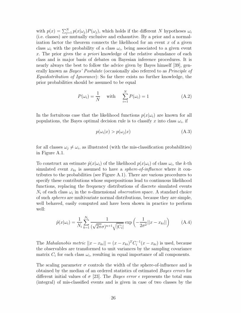
In the fortuitous case that the likelihood functions p(x|ωi) are known for allpopulations, the Bayes optimal decision rule is to classify x into class ωi, if
p(ωi|x) > p(ωj |x) (A.3)
for all classes ωj 6= ωi, as illustrated (with the mis-classification probabilities)in Figure A.1.
To construct an estimate p(x|ωi) of the likelihood p(x|ωi) of class ωi, the k-thsimulated event xki is assumed to have a sphere-of-influence where it con-tributes to the probabilities (see Figure A.1). There are various procedures tospecify these contributions whose superpositions lead to continuous likelihoodfunctions, replacing the frequency distributions of discrete simulated eventsNi of each class ωi in the n-dimensional observation space. A standard choiceof such spheres are multivariate normal distributions, because they are simple,well behaved, easily computed and have been shown in practice to performwell:
p(x|ωi) =1
Ni
Ni∑
k=1
1
(√2πσ)n+1
√
|Ci|exp
(
− 1
2σ2||x− xki||
)
(A.4)
The Mahalanobis metric ||x− xki|| = (x− xki)TC−1
i (x− xki) is used, becausethe observables are transformed to unit variances by the sampling covariancematrix Ci for each class ωi, resulting in equal importance of all components.
The scaling parameter σ controls the width of the sphere-of-influence and isobtained by the median of an ordered statistics of estimated Bayes errors fordifferent initial values of σ [23]. The Bayes error ǫ represents the total sum(integral) of mis-classified events and is given in case of two classes by the
26
p
Fe
p(x|
ωi)
Arb. Units
p(x|ωp)
Pp→Fe
p(x|ωFe)
PFe→p
p(x|
ωi)
Arb. Units
0
0.1
0.2
0.3
0.4
0.5
0.6
0.7
0.8
0.9
3 4 5 6 70
0.2
0.4
0.6
0.8
1
3 4 5 6 7
Fig. A.1. Schematic illustration of the construction of two one-dimensional (over-lapping) likelihood functions p(x|ωp,Fe), approximated by Gaussian distributions(sphere-of-influence) for each event, indicated on the abscissa (left). Classificationusing the Bayes decision showing the proportion of mis-classified events by thehashed areas (right) (P (ωFe) = P (ωp)) .
simple relation ǫ =∫
min{p(ω1|x), p(ω2|x)} · p(x) dx (hatched areas in Fig-ure A.1 right). To account for the mis-classification, the rates Pij = Pωi→ωj
,i.e. the probability of an event x ∈ ωi being classified in the class ωj, are esti-mated by the leave-one-out method (also called jack-knifing). Each simulatedevent is held back once while the others are used to estimate the associationof this particular event. By a, so called, bootstrap method different subsets ofeach simulated class are used to perform the leave-one-out method to give anasymptotically unbiased estimate of the variance of the Pij [36]. Thus the truenumber of events n⋆
i can be deduced from the classified events nj by a matrixinversion:
∑
j
P−1ij nj = n⋆
i with Pij = Pωi→ωj(A.5)
A.2 Neural networks
An artificial neural network can be considered as a nonlinear transfer function
f : Rp −→ Rq (A.6)
mapping a bounded euclidian space of dimension p to another space of dimen-sion q. The, so called, multilayer feed-forward neural network is organized inL different layers: an input layer, L − 2 hidden layers, and an output layer.Each layer l consists of a certain number nl of units (neurons), which carry
27
on the signals to the next layer. The, so called, network topology specifies thenumber of units in each layer: n1 × n2 × . . .× nL−1 × nL. An output unit ymL
of the output layer L is determined for each observation vector (input units)xki and class ωi entering the input layer and should be close to the true valuetki, given by the labeled simulation events in terms of a well defined measure.Thus, the error function E(w)
E(w) =1
2
N∑
i=1
1
Ni
Ni∑
k=1
(ymL(xki,w)− tki)2 (A.7)
has to be minimized. For each layer l, except of the input, the outcome ofeach neuron m is calculated by a weighted sum of the output of neurons ofthe last preceding layer. Additionally an activation function f(z) is applied tothe sum
yml = f(z) = f
(nl−1∑
i=1
wmi,l−1 · yi,l−1 + wm
l
)
. (A.8)
A convenient practice is to use the Fermi function f(z) = 1/(1 + exp(−z)).The most common algorithm for the network training, i.e. minimizing E(w), isan adjustment of the weights wm
i,l−1 and wml by a stochastic minimization pro-
cedure [23] or alternatively by the, so called, back-propagation algorithm [40].There exist different other algorithms or extended versions of this basic back-propagation, which try to circumvent problems in finding the global minimumor sticking in a local minimum. Additional problems arise, if the training pro-cess leads to an overtraining of the network by adopting the properties of thetraining samples, but cannot give satisfactory results, when it is applied toanother validation set. Thus, in a generalization phase one has to control thequality of the network with an independent labeled set of samples.
In general, the output ymL is a continuous function. Hence not only the classi-fication can be done applying neural networks, but also parameter estimation(regression) is possible, e.g. the estimation of the primary energy of EASevents. In case a classification into N classes is required, the output ymL ofthe network is divided into N regions, each representing a single class [23].
In previous publications the consistency and equivalence of neural network andBayes classifier results in EAS analysis have been demonstrated [24,25]. Theclassification rates Pij inferred from both procedures do not differ significantly.Thus, an adequate choice of the particular decision rule and of the appropriatealgorithm is just a matter of the actual conditions like computing time andmemory workload.
28