Embed Size (px)
Citation preview
PHYSICSREPORTS(Review Sectionof PhysicsLetters)156, No. 4 (1987) 147—225.North-Holland, Amsterdam
ANOMALOUS SCALING LAWS IN MULTIFRACTAL OBJECTS
Giovanni PALADIN and Angelo VULPIANI
Dipartimento di Fisica, Università di Roma“La Sapienza”, P. le A. Moro 2, 00185Roma,italy
and
GNSM-CISMRoma,Italy
ReceivedMay 1987
Contents:
0. Introduction 149 3.6. A thermodynamicalformalism for unidimensional-1. Chaoticattractorsas inhomogeneousfractals 152 maps 192
1.1. Why study attractors’dimensions? 152 3.7. Partialdimensionsand entropies 1951.2. Characterizationof chaoticattractorsas multifractal 4. Replicasof disorderedsystemsasmultifractal objects 198
objects 157 4.1. Introduction 1981.3. Othercharacterizationsof attractorsandexperimental 4.2. The one-dimensionalAndersonmodel 199
problems 161 4.3. Anomalousscalinglaws at the bandedge 2022. Intermittencyin fully-developedturbulence 162 4.4. Freeenergyfluctuationsin spin glasses 205
2.1. Basicconceptson fully-developedturbulence 162 5. Multifractal structuresin condensedmattersystems 207.2.2. Kolmogorovtheory and the intermittencyproblem 164 5.1. Generalremarks 2072.3. Fractalandmultifractal modelsfor intermittency 166 5.2. Multifractal wavefunctionat the localizationthreshold 2082.4. Remarksand consequencesof multifractality in tur- 5.3. Growth probability distributionin kinetic aggregation
bulence 172 processes 2122.5. Two-dimensionalturbulence 176 5.4. Multifractality in percolation 215
3. Temporalintermittencyin chaotic dynamicalsystems 177 6. Conclusions 2173.1. Generalremarks 177 AppendixA. The Kolmogorov—Obukhovlognormal model3.2. GeneralizedLyapunovexponents 179 for intermittencyin turbulence 2183.3. The Renyi entropies 185 AppendixB. Multiplicative processesandlognormalapproxi-3.4. Relation between the generalizedLyapunov expo- mation 220
nentsandthe Renyi entropies 187 References 2223.5. Multifractality in thetrajectory space 189
Singleordersfor this issue
PHYSICSREPORTS(Review Sectionof PhysicsLetters)156, No. 4 (1987) 147—225.
Copiesof this issue may be obtained at the price given below. All ordersshould be sentdirectly to the Publisher.Ordersmust beaccompaniedby check.
Single issue price Dfl. 56.00, postageincluded.
0 370-1573/87/$27.65 © ElsevierSciencePublishersB .V. (North-HollandPhysicsPublishingDivision)
ANOMALOUS SCALING LAWS INMULTIFRACTAL OBJECTS
Giovanni PALADIN and Angelo VULPIANI
Dipartimento di Ficica, Università di Roma “La Sapienza”,P. leA. Moro 2, 00185 Roma, Italy
and
GNSM-CISMRoma, Italy
INORTH-HOLLAND - AMSTERDAM
G. Paladin and A. Vulpiani, Anomalousscaling laws in multifractal objects 149
Abstract:Anomalousscaling laws appearin a wide class of phenomenawhere global dilation invariancefails. In this case,the descriptionof scaling
propertiesrequiresthe introduction of an infinite setof exponents.Numerical and experimentalevidence indicates that this descriptionis relevantin the theory of dynamical systems,of fully developed
turbulence,in the statistical mechanicsof disorderedsystems,and in somecondensedmatterproblems.We describeanomalousscalingin termsof multifractal objects.They aredefinedby a measurewhosescalingpropertiesarecharacterizedby a
family of singularities,whichareidentified by a scalingexponent.Singularitiescorrespondingto thesameexponentaredistributedon a fractalset.The multifractal objectarisesas the superpositionof thesesets, whose fractal dimensionsare relatedto the anomalousscalingexponentsvia aLegendretransformation.It is thus possible to reconstructthe probability distributionof thesingularity exponents.
We reviewthe applicationof this formalismto the descriptionof chaoticattractorsin dissipativesystems,of the energydissipatingset in fullydevelopedturbulence,of someprobability distributions in condensedmatterproblems.Moreover,a simpleextensionof the methodallows us totreat from the samepoint of view temporalintermittency in chaotic systemsand sampleto samplefluctuationsin disorderedsystems.
We stress the phenomenologicalnatureof the approachand discussthe few casesin which it was possible to reach a more fundamentalunderstandingof anomalousscaling.We point out theneedof atheorywhichshouldexplainitsorigin andpavethewayto amicroscopiccalculationof the probability distributionof the singularities.
Jo fingo esuppongoche qualchecorpo si muovaall’ insi~secondola notaproporzioneet orizzontal-menteconmotoequabile...Sepoi lepalle di piombo,di ferro, di pietra, non osservanoquella suppostadirezione,SUO danno: fbi
diremo che non parliamo di esse.
I feign andassumethat somebodiesmovevertically accordingto the knownratio, andhorizontallyby uniform motion...If balls madeof lead, iron or Stone do not comply to thisrule, it is all to their disadvantage:for weshallsay thatwe are not talking of them.
EvangelistaTorricelli
0. Introduction
Scaling invarianceplaysa fundamentalrole in many naturalphenomenaandis often relatedto theappearanceof irregularforms which cannotbedescribedby the usualdifferentialgeometry.A classicalexampleis given by the Brownianmotion the studyof which led JeanPerrin [P06,P13] to understandthe physical relevanceof non-differentiablecurvesand surfaces.
Thenecessityof introducinga new classof geometricalobjects,the fractals,hassubsequentlyarisenin various different problems.Indeed,someaspectsof ‘fractality’ werealreadypresentin the ideasofsomeScientistsat the beginning of this centurylike Perrin himself, Besicovitch,Hausdorff, Wiener,Richardson,but the concept of ‘fractal object’ was explicitly formulated and madepopular in thescientific communityin recentyearsby Mandeibrot.
The main ideaconsistsin the characterizationof the scalingstructureof an objectby meansof anindex, the fractal dimensionDF which coincidesfor ‘ordinary’ shapeswith the usual (topological)dimensionDT. Indeed,the dimensionalityof objectscan be definedin differentways. Onecan defineitas a topological conceptby counting the numberof independentdirectionsin which one can movearound any given point (for a rigorous definition see,e.g., [ER85]). One can call this notion thetopologicaldimension.On the otherhand,wecan definethe fractal dimensionas a ‘capacity’ measureby consideringthe numberN(l) of hypercubesof edgeI necessaryto coveran objectembeddedin aD-dimensionalspacein the limit l—+0:
N(l)c~~l’~. (0.1)
150 G. Paladin andA. Vulpiani, Anomalousscaling laws in multifractalobjects
It follows that DF ~ D and the objectis called fractal if DF> DT.The fractal dimensionis purely geometrical,i.e. it only dependson the shapeof the object. In
general,one hasto assignto the physical object a suitableprobability measuredis, accordingto theparticular phenomenonconsidered.
The measured~tshouldscalewith the resolution length. Let usdefine a coarsegrainedprobabilitydensity
p~(l)= f d~(x) (0.2)
as the ‘mass’ of the hypercubeA~of size 1, With = 1, 2,. . . N(l). The scaling rate is given by theinformation dimensionD1 definedby Balatoni and Renyi [BR56]:
N(l)
p, ln(p1) D1 ln(l). (0.3)
One can easily show that D1 ~ DF where the equality is valid only for a uniform distributionp~= 1IN(l)ccl’~for eachbox A1.
D1 is a more interestingindex thanDF. It must be noted, in fact, that the numberNR(l) of boxescontainingthe dominantcontributionsto the total mass,andthusthe relevantpart of the information,is:
NR(l) (0.4)
as consequenceof the Shannon—McMillantheorem (seee.g. [K57]).If D1 < DF, then the measureitself is called fractal [F82] since it is singular with respectto the
uniform distributionp~ i.e. p2 Ip ~can divergein the limit of vanishing1. The supportof the measureisin this sensean inhomogeneousfractal object.
The principal aimof this reviewis to characterizedifferentphysicalsystemsby meansof the analysisof the probability measuresingularities.The understandingof thejr structurecan be actually achievedby extractingfrom experimentsor simulationsthe ‘mass’ momentscaling
N(1)
~~(l)~) p(j)~l+l ~ (0.5)The dq are the Renyi dimensionswhich generalizethe information dimensionD1 = d1 as well as thefractal dimensionDF = d0. If the fractal is homogeneous,thenone can extractq out of the averageoperationin (0.5) and the Renyi dimensionsare thereforeall equalto the fractal dimension.On thecontrary, if the dq ‘s arenot constant,one speaksof anomalousscalingand, as the orderq varies, theamount of the difference dq — DF gives a first rough measurementof the inhomogeneity of theprobabilitydistribution. Suchabehaviourarisesin many differentsystemsandwas first pointedout byMandelbrot[M74] in fully developedturbulence.SubsequentlyParisi andcoworkers[FP85,BPPV84]introduced the conceptof multifractal object in the samecontext, realizing that the moment scalingindicescanbe relatedto thescalingof the probability distributionof the singularities The objectcan beregardedin this approach,further developed~y Halseyet a!. [HJKPS86,JKLPS85],as an interwovenfamily of differenthomogeneousfractal setsS(a) on which the measurehasa singularity of typea (i.e.p2(l) ~ l’~for boxesA, belonging to S(a)). It is possibleto relate the Renyi dimensions(which can bedirectly measuredin experiments)to the fractal dimensionsf(a) of the setsS(a) (or equivalentlyto theprobability of picking up a singularity a with resolutionscale1) via a Legendretransformation.
G. Paladin andA. Vulpiani, Anomalousscaling laws in multifractal objects 151
This is the heartof the methodwhich hasbeenalso appliedto the studyof the momentsof genericobservablesA computedon scale1:
(A(l)~) i~.
Despiteits name,anomalousscaling,i.e. a non-linearshapeof the functiong( q), is the morecommonsituation even if it contrastswith the standard ideas about critical phenomenawhere one usuallyconsidersonly a finite numberof scaling exponents.
Moreover the same object can be a multifractal with respect to a certain observableand ahomogeneousfractal with respectto anotherone. The readercan find an explicit exampleof such afeaturein section2.
Up to now we havelookedat multifractality as the manifestationof the spatial fluctuationsof theobservables.Nevertheless,temporal scaling featuresappear of great importance in the chaoticevolutionof deterministicdynamicalsystems.In thesecasesoneusuallyobservesstrongtime variationsin the degreeof chaoticity. This intermittencyphenomenoninvolvesan anomalousscalingwith respectto ‘time dilations’ identifying the parameterexp(—t) with the parameter1 used in spatial dilations. Ameasureof the degreeof intermittencyrequiresthe introductionof infinite setsof exponentswhich areanalogousto the Renyi dimensionsandcan be relatedto a multifractalstructuregiven by the dynamicalsystemin the functional trajectoryspace.
In section1 we introducethe multifractal formalismin the contextof dissipativedynamicalsystems.We define the Renyi dimensionsof the naturalmeasuregeneratedby a deterministicevolutionlaw
on a chaotic attractor and describethe numericalalgorithms for their calculation. Indeed, typicalchaoticattractorscan be regardedas multifractal objects.We discussin detail how the scalingof theprobability that a point of the attractor(representativeof the stateof the dynamicalsystem)belongstoS(a) is determinedby the fractal dimensionalityf(a) of S(a)andwe point out that thereis asingularityhierarchythe top of which is given by the information dimensionD1.
If the attractor is homogeneous,the natural measureis not fractal and has only a singularitya = DF = D1 with respectto the Lebesguemeasureand dq = DF, Vq.
In section2 we apply this approachto the study of the statisticalpropertiesof fully developedturbulencewhere there is spatial intermittency of the energydissipatione(x) implying anomalousscalinglawsfor the momentsof thevelocity differences,the so-calledstructurefunctions.Intermittencycan be reproducedby modelsassumingthat s is concentratedon fractal structureswith DF ~ 3.
One may thenconsiderr as a mass densityand a non-homogeneousdistribution correspondstoanomalousscalinglaws as in chaoticattractors.This allowsus to extendthe resultsof section1 to thecharacterizationof the singularitiesof s.
We introducea multiplicative process(random/3-model) for building-upa propermultifractal objectandthusobtaina good fit to the experimentaldata with only one adjustableparameteron the basis ofphenomenologicalassumptions.
We also emphasizethat the multifractal nature of turbulencedoesnot affect in a substantialwaysomephenomenalike the separationof particlepairswhereasit is relevantin determiningthe numberof degreesof freedominvolved.
Section3 showshowthe degreeof temporalintermittencyof the chaoticityin adynamicalsystemcanbe measuredby indiceswhich areextractedeither by an experimentalsignal (the Renyi entropiesKq)or by numericalcalculations(the generalizedLyapunovexponentsL(q)).
The multifractal approachcan be extendedto the study of ‘temporal inhomogeneities’with slight
152 G. Paladin andA. Vulpiani, Anomalousscaling laws in multifractal objects
modifications and it allows to reconstruct the probability distribution which rules the temporalfluctuationsaroundthe averagedegreeof chaoticitymeasuredby the Kolmogorov entropyK1 andthecharacteristicLyapunovexponents.We alsogive someexamplesof numericalcalculationsof the L( q)’sin dynamicalsystemswith few degreesof freedom.
We finally discussthe caseof one-dimensionalchaoticmapswhichhighlights the relationbetweenthemultifractal methodand the thermodynamicformalism introducedfor hyperbolicsystemsby Bowen,Ruelle, Sinai andWalters. In this framework we show that the appearanceof edgesin the Renyientropiesis an indication of phasetransitions.
In section4 the techniquesdevelopedfor the characterizationof the chaoticbehaviourof dynamicalsystemswill be usedin the studyof the trajectoriesgivenby the productsof randomtransfermatrices.They can,e.g., describethe localizationof the wavefunction of the Schroedingerequationin a randompotentialor the partition function of spin glasses.Themultifractal approachis in thiscasethe analogueof the usual statistical theory of finite volume fluctuations of the physical observables(we shallrespectivelyconsiderthe localizationlengthandthe free energy)amongdifferent replicasof the samesystemwith respectto disorder.The calculationof thegeneralizedLyapunovexponentsthereforegivesthe possibility to reconstructthe scaling propertiesof the probability distribution of the observables.The massdensityis the densityof replicascharacterizedby the sameobservablevaluecorrespondingtotrajectorieswith the samedegreeof chaoticity, andin this sensethereplicasdefinea multifractal objectin the realizationspace.
In section5 we analysesomecritical phenomena(localizationtransitionand conductionin randomresistornetworks at the percolationthreshold)as well as somegrowth phenomena(diffusion limitedaggregation)wherea hierarchyof differentexponentsappearsas a new interestingfeature.We stressthe fact that, approachingthe critical point, the probability of finding scalingexponentsdifferent fromthat correspondingto the information dimensiontendsto zero as a power of correlationlength.
In section6 the readerwill find someconcludingremarks.
1. Chaotic attractors as inhomogeneousfractals
1.1. Whystudyattractors’ dimensions?
Recently,it hasbeenshownthatdeterministicevolutionlawsmayleadto chaoticbehaviourseveninabsenceof externalnoise [LL83, ER85]. This phenomenon,called deterministicchaos,is essentiallydueto a sensitivedependenceon initial conditionsand hasagreatrelevancein the descriptionof manyphysicalsystemswhose dynamicscan be modelledby ordinary differentialequationsor maps:
dxldt =f(x(t)) , x(i + 1) = g(x(i)) (1.1.1)
with x,f, gER’~.One of the first exampleswas given by Lorenz [L63] who showedthata dynamicalsystemof just
threedifferentialequationscan be chaotic.In this sectionwe limit ourselvesto the studyof the attractorsof dissipativesystemsbut manyresults
can also be applied to genericchaoticsignals.Indeed,after a transient,a dissipativesystemusuallyevolvesin the neighbourhoodof a setcalled attractor(for a rigorousdefinition see,e.g., [ER85]).
The conceptof dimensionis relevantfor the dynamicsbecauseit providesa preciseway to estimatethe numberflf of independentrelevantvariablesinvolved in the evolution.
G. Paladin andA. Vulpiani, Anomalousscaling laws in multifractalobjects 153
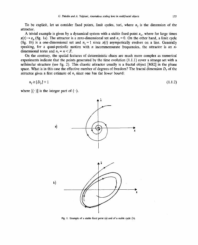
To be explicit, let us consider fixed points, limit cycles, tori, where n~is the dimensionof theattractor.
A trivial exampleis given by a dynamicalsystemwith astablefixed point x0, wherefor largetimesx(t)—s~x0 (fig. la). The attractoris a zero-dimensionalsetand flf = 0. On the otherhand,a limit cycle(fig. ib) is a one-dimensionalset and flf = 1 since x(t) asympoticallyevolves on a line. Generallyspeaking,for a quasi-periodicmotion with n incommensuratefrequencies, the attractor is an n-dimensionaltorus and flf = n < F.
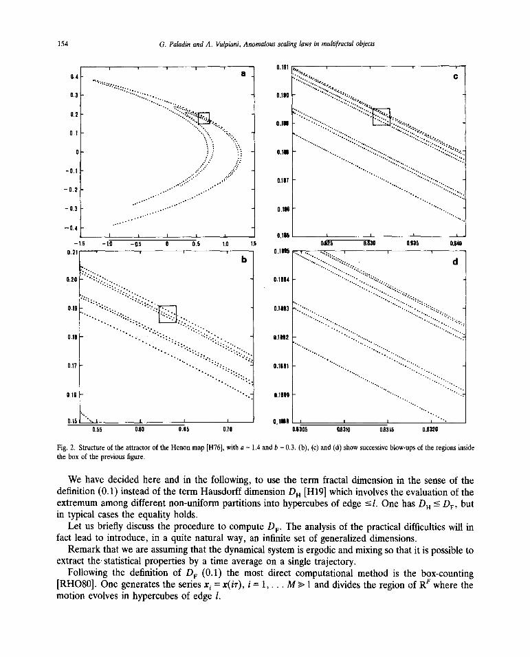
On the contrary, the spatial featuresof deterministicchaosare much more complex as numericalexperimentsindicatethat the pointsgeneratedby the time evolution(1.1.1)cover a strangesetwith aselfsimilar structure(see fig. 2). This chaoticattractorusually is a fractal object [M82] in the phasespace.What is in this casethe effectivenumberof degreesof freedom?The fractal dimensionDF of theattractorgives a first estimateof n~since onehasthe lower bound:
� [DF] + 1 (1.1.2)
where [(S)] is the integerpart of (S).
a) __
Fig. 1. Exampleof a stable fixed point (a) andof a stablecycle (b).
154 G. Paladin and A. Vulpiani, Anomalousscaling laws in multifractalobjects
I ~0.4 ~ a - ~ C
03 0180
-~ :;0117
—0.2 ........... . ...-.-....
-0.3 .... .............- 0.111-
—0.4 -.
I I I I 0.115 I I
—1.5 —1.0 —0.5 0 0.5 1.0 15 0.125 0.830 0.635 0.5400.21 • I 0.1115 ..~,...~
b d
020 01114
019 0103
018 01112
017 01591
0.16 0.1880 - ......-..
0.15~._I I I 01118 I I
0.55 0.80 0.85 0.10 0.6305 0.6310 0.8315 0.6320
Fig. 2. Structureof the attractorof theHenonmap[H76},with a = 1.4 andb = 0.3. (b), (c) and(d) showsuccessiveblow-upsof theregionsinsidethe box of theprevious figure.
We havedecided hereand in the following, to usethe term fractal dimensionin the senseof thedefinition (0.1) insteadof the term HausdorifdimensionDH [H19]which involvesthe evaluationof theextremumamongdifferent non-uniformpartitionsinto hypercubesof edge� I. OnehasDH ~ DF, butin typical casesthe equality holds.
Let us briefly discussthe procedureto computeDF. The analysisof the practicaldifficulties will infact leadto introduce,in a quite naturalway, an infinite setof generalizeddimensions.
Remarkthat we areassumingthat the dynamicalsystemis ergodicandmixing sothat it is possibletoextractthe’ statisticalpropertiesby a time averageon a single trajectory.
Following the definition of DF (0.1) the most direct computationalmethod is the box-counting[RHO8O].One generatesthe seriesx, = x(ir), i = 1,. . . M ~‘ 1 anddividesthe region of RF wherethemotion evolvesin hypercubesof edge1.
G. Paladin andA. Vulpiani, Anomalousscaling laws in multifractal objects 155
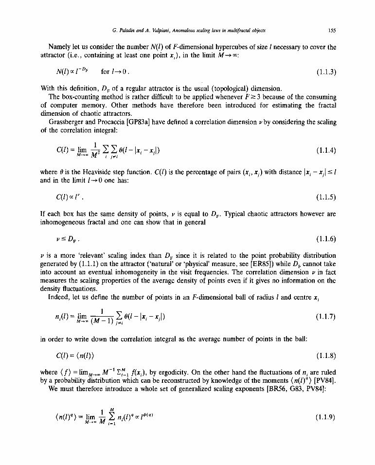
Namelylet us considerthe numberN(l) of F-dimensionalhypercubesof size 1 necessaryto cover theattractor(i.e., containingat least onepoint x.), in the limit M—~m:
N(1)ccl’~ for l—tO. (1.1.3)
With this definition, DF of a regularattractoris the usual (topological)dimension.The box-countingmethodis ratherdifficult to be appliedwheneverF~ 3 becauseof the consuming
of computer memory. Other methods have therefore been introduced for estimating the fractaldimensionof chaoticattractors.
GrassbergerandProcaccia[GP83a]havedefinedacorrelationdimensionv by consideringthe scalingof the correlationintegral:
C(l)=hm —~-i~~0(l—Ixt—x1l) (1.1.4)—‘=M ,
where0 is the Heavisidestepfunction. C(1) is thepercentageof pairs(x,, x~)with distance x, — � 1and in the limit l—~0 one has:
C(l) l~. (1.1.5)
If eachbox hasthe samedensityof points, v is equalto DF. Typical chaoticattractorshoweverare
inhomogeneousfractal and one can showthat in generalx1�DF. (1.1.6)
v is a more ‘relevant’ scaling index than DF since it is relatedto the point probability distributiongeneratedby (1.1.1)on the attractor(‘natural’ or ‘physical’ measure,see[ER85])while DF cannottakeinto accountan eventualinhomogeneityin the visit frequencies.The correlationdimension ii in factmeasuresthe scalingpropertiesof the averagedensityof pointseven if it gives no information on thedensityfluctuations.
Indeed,let us definethe numberof points in an F-dimensionalball of radius1 and centrex1
n~(l)= lim1M— ~ ~ 0(1 — x
1 — x11) (1.1.7)M—~oc~
in order to write down the correlationintegralas the averagenumberof points in the ball:
C(1) = (n(l)) (1.1.8)
where (f) = limM.,~,M - ~ f(x,), by ergodicity. On theotherhandthe fluctuationsof n, are ruledby a probabilitydistributionwhich canbe reconstructedby knowledgeof themoments(n(l)~)[PV84].
We must thereforeintroducea whole set of generalizedscalingexponents[BR56,G83, PV84]:
(n(l)’~) lirn ~ ~ n.(i)~o~i”~-~ (1.1.9)
156 G. Paladin andA. Vulpiani, Anomalousscaling laws in multifractal objects
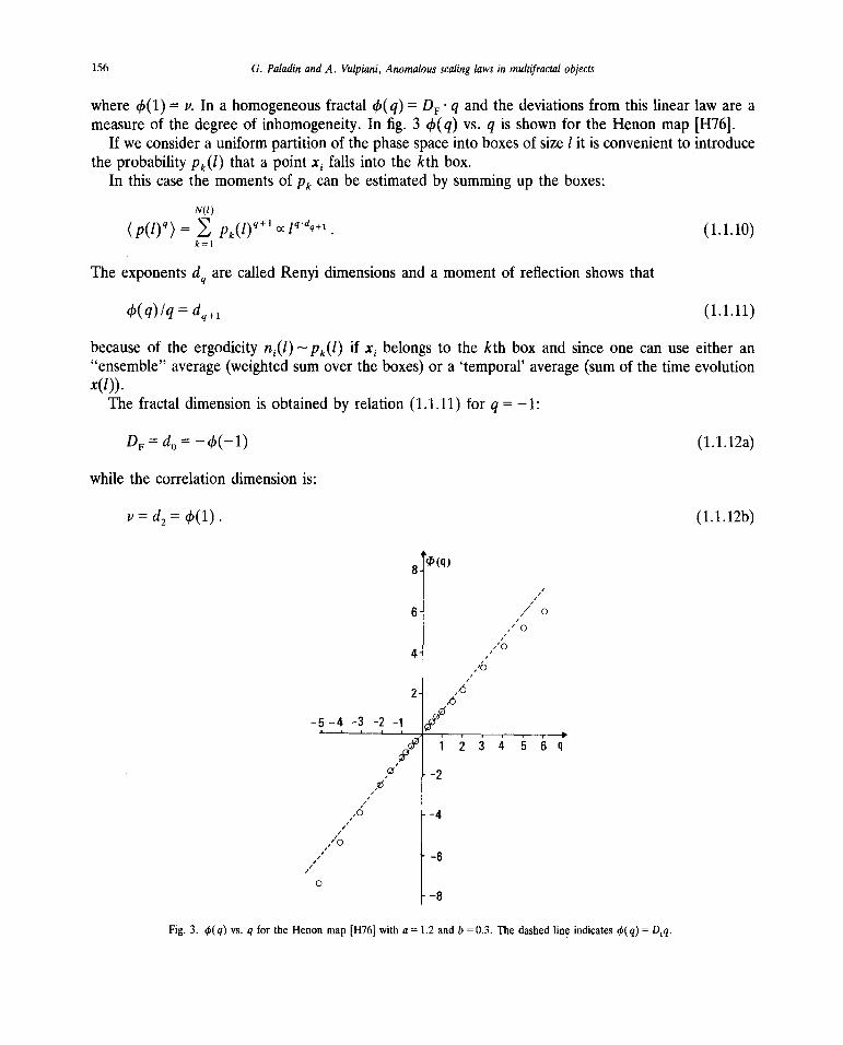
where4(1) = ii. In a homogeneousfractal ~( q) = DF q andthe deviationsfrom this linear law areameasureof the degreeof inhomogeneity.In fig. 3 4(q) vs. q is shownfor the Henon map [H76].
If we considera uniform partition of the phasespaceinto boxesof size lit is convenientto introducethe probability Pk(I) that a pointx~falls into the kth box.
In this casethe momentsof Pk can be estimatedby summingup the boxes:
N(1)
= Pk(l) ~q.dq+i (1.1.10)
The exponentsdq are calledRenyi dimensionsand a momentof reflection showsthat
4(q)Iq=dq~1 (1.1.11)
becauseof the ergodicity n,(l) —~Pk(l) if x, belongsto the kth box and since one can useeither an“ensemble”average(weightedsumover the boxes)or a‘temporal’ average(sum of the time evolutionx(l)).
The fractal dimensionis obtainedby relation (1.1.11)for q = —1:
DF = d0 = —4(—1) (1.1.12a)
while the correlationdimensionis:
~.‘=d2= 4(1). (1.1.12b)
-5—4 —3 -2 —1
4 ~
Fig. 3. 41(q) vs. q for the Henonmap[H76l with a = 1.2 and b = 0.3. The dashedline indicates41(q) = D1q.
G. Paladin and A. Vulpiani, Anomalousscaling laws in multifractal objects 157
Onecan alsoshow that q5(q) is a convexfunction of q by a generaltheoremof probability theory [F71]anddq consequentlydecreasesas q increases.
A numericalcomputationof the Renyi dimensionshasto be performedfollowing the definition(1.1.9) instead of (1.1.10). It is in fact easy to generalizethe Grassberger—Procacciamethodforcomputingthe momentsof n,(l) with atime-consumingof thesameorderas thatfor computingv, whilethe memory-consumingproblemsof the box-countingmethodare escaped[PV84].
Other ways exist for introducingan infinite set of dimensions;Hentscheland Procaccia[HP83a],e.g., proposedthe following characterizationof the attractors.Let usdefine:
C0(1) = lirn [numberof n-tupletsof points (x,, x,,. . . x~)
whosedistances x, — xJ are lessthan 1 for all i~,i~] (1.1.13)
which should scaleas:
C~(l)ccl” forsmalll (1.1.14)
with v2 = i.’. Note that the direct computationof i~,following the definition (1.1.13)requiresa CPUtimeincreasingas M~.Howeverit is easyto recognizethat
v~=(n—1).d0, n=2,3,4 (1.1.15)
The relation (1.1.15)is obtainedby the fact that in the ith box the distributionof pointsis essentiallyuniformimplying
C~(1) = [numberof n-tupletsof points (x1,. . . x,) containedin the ith box with all — xJ � 1] cep~(l)’
1M~. (1.1.16)
(1.1.15) follows from (1.1.10),(1.1.13)and (1.1.16)sinceC~(l)= lim(1IM) ~ C~(l).
1.2. Characterizationof chaoticattractors as multifractal objects
It is intuitively reasonablethat the dimensionsdq give a measureof inhomogeneityin the distributionof pointson the attractor.Let us nowshowhowthis inhomogeneitycan berelatedto the existenceof aspectrumof singularitiesof the naturalmeasure.
Let us cover the attractorwith N(l) boxesof edge1 and define the probability p.(l) that a pointbelongsto the ith box A,(1)
p~(l)= f d~(x). (1.2.1)A~(1)
d~(x)is the naturalmeasuregiven by the dynamics. In practice,in a numericalexperimentp,(l) isgiven by ~k (I) defined in (1.1.7) with ‘k centredin A.(l). In the limit of a homogeneousattractor,p,(l) ~ ~ while this doesnot happenin a genericcase. Let us thereforegroup the boxeswith thesingularity i E [a, a+ da]:
158 G. Paladin and A. Vulpiani, Anomalousscaling laws in multifractal objects
p,(l)r,~la for small 1 (1.2.2)
into a subsetS(a) of the attractor. Roughlyspeakinga is a ‘local massdimension’.The numberof boxesdNa(l) neededto coverS(a) should behavein the scaling hypothesislike:
dNa(l)= dp(a) ~ (1.2.3)
wheref(a) arethe different fractal dimensionsof the setsS(a)upon which the singularitiesareof kinda. Essentiallywe aredescribingthemeasureon the attractorby interwovensetseachwith singularityofkind a andfractal dimensionf(a).
Now we can relatef(a) to dq by computingthe quantities(1.1.10)as an integralon a. Followingequations(1.2.2, 1.2.3) one has:
N(1)
~ ~(l)~ f dp(a)l~. (1.2.4)
The integral can be computedfor small 1 by the saddlepoint method:
dq = (q -1) m~n(aq -f(a)). (1.2.5)
If we knowf(a), thenwe can find dq and, alternatively,givendq, we obtainf(a) inverting (1.2.5). Inthe limit caseof homogeneousattractorsf(a) is defined only for a = DF implying f(DF) = DF anddq = DF, Vq.
The meaningof (1.2.5) is quite obvious:dq is detectedby aparticularvalueof ã(q) determinedbythe extremumconditionsof (1.2.5):
df/daL~= q(i) (1.2.6)
and
1 — —
dq = (q —1) [cia —f(a)]. (1.2.7)
One has the obvious inequality f(a) ~ DF becauseNa(1) ~ N(l), while the information dimensionD1 = d1 satisfiesthe relation
D1=f(D1). (1.2.8)
We can repeatthe above computationsfor the exponents(1.1.9) by a summationover the pointsinsteadof over the boxes.Thisdescriptionis exactlyequivalentbut allows to emphasizecertainphysicalaspects.Let us introducethe percentageof pointsXa(l) which belongsto the boxesof size 1 suchthat(1.2.2) holds:
dXa(l) ~ dNa(l) l~~dp(a) lH(~ (1.2.9)
G. Paladin and A. Vulpiani, Anomalousscaling laws in multifracial objects 159
with
H(a)a—f(a)�0. (1.2.10)
By (1.1.9) and (1.2.9) it follows
(fl(j)q) ~fdp(a) /aq+H(a)
and one obtains
~(q) = qdq~1= mm [aq + H(a)]. (1.2.11)
For q = 0, we selectthe informationdimensiond1 = d4ildqIq.~0correspondingto the singularitya =
for whichH = 0. In the limit 1—~0 all the pointswith a~ D1 cannotbe detectedsinceXa vanisheswith I
for positiveH(a). This situationis well knownin theframeworkof informationtheory. Indeed,we gainan information1(l) = —~ p,(l)ln p,(l) in a measurementof the systemstatewith precision1. TheShannon—McMillantheorem [K57] assuresthat the number NR(l) of boxeswhich give the leadingcontributionto 1(1) should scalelike i’d’ D1 is thereforethe mostprobable‘local massdimension’, ifwe pick up the points accordingto the naturalmeasure.This fact haspracticalconsequencesin theanalysisof experimentalsignalswhereoneusually computesthe correlationdimensionson a small setof points, let usdefine ~ as
~=ln(-~ kl nk(l))/lnl
whereonechoosesM pointsXk at randomamongthe M pointsx1, x2,. . . XM of the temporalsequence[ER85]. If M is much smaller than M, then i~is closer to D1 rather than to v. We think thatexperimentalistsshould take into account this warning for the estimationof the dimensionof anattractor.
The Legendretransform becomessimple also in the limit q—~ + ~ where the minimum conditionpicks up the extremevaluesof the singularities:
amax = q
1!~oodq; amjn = q~r~0,dq~ (1.2.12a)
For q large enough(say q> q1 >0, q< q2 <0), the function 4(q) reachesits asymptoticbehaviour:
~(q) a~j~q+ H(~mjn)for q > q1(1.2.12b)
+ H(amax) for q < q2.
Let us notethatf(a) can be negative.In thiscasethefractal dimensionof the correspondingsetS(a) iszero,of courseandS(a) is called ‘volatile’ fractal [M82].Negativef(a)’s indicatehow fast the numberof boxesnecessaryto coverS(a) convergeto zero in the limit of vanishingsize 1.
Analytical calculationsof some featuresof f(a) have been performedjust on particular scale-
160 G. Paladin and A. Vulpiani, Anomalousscalinglaws in multifracial objects
invariant structures(such as the 2-cycle of period doubling,mode-locking structures,quasi-periodictrajectoriesfor circle maps) [HJKPS86,K86].
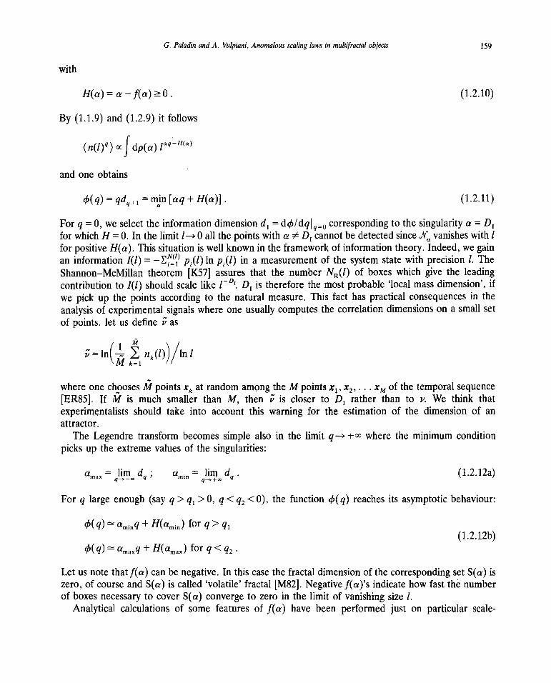
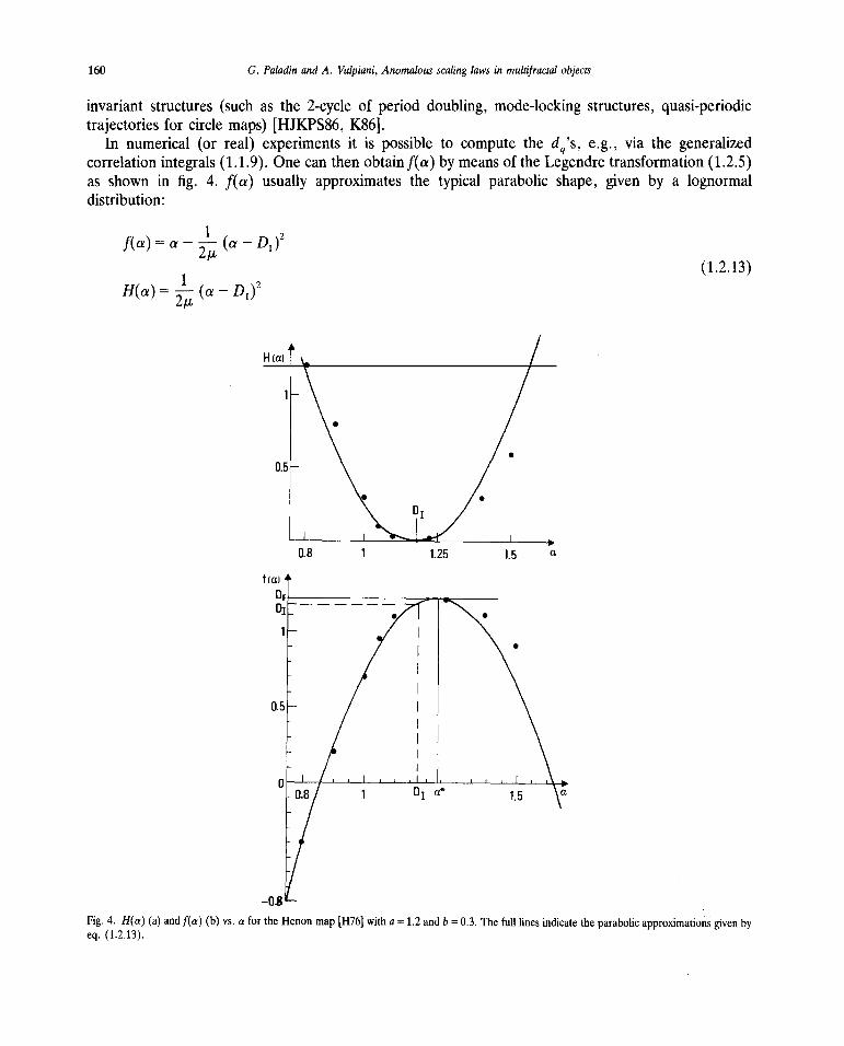
In numerical (or real) experimentsit is possible to computethe dq’5~e.g., via the generalizedcorrelationintegrals(1.1.9). Onecan thenobtainf(a) by meansof the Legendretransformation(1.2.5)as shown in fig. 4. f(a) usually approximatesthe typical parabolicshape,given by a lognormaldistribution:
f(a)a_~~(a_Di)2
(1.2.13)H(a)
Ht1L1s~DIl./l: ~
(a)
S
05— I
~U.8 1 01a 1.5 a
-M -
Fig. 4. H(a) (a) andf(a) (b) vs. afor theHenon map[H76l with a = 1.2 andb = 0.3. The full linesindicatetheparabolicapproximationsgiven byeq. (1.2.13).
G. Paladin andA. Vulpiani, Anomalousscaling laws in multifractalobjects 161
and ~ is given by
= lim (ln2(n(l)) — (ln(n(l)))2) (1.2.14)Iln l~
We shall discussin the appendixB the limits of this approximation.However, for small q one hasingeneral:
dq+i=d1~~ILq. (1.2.15)
1.3. Other characterizationsof attractorsand experimentalproblems
The methodsdevelopedin sections1.1 and 1.2 arerelatedto the statisticalpropertiesof p,(1) in thelimit of infinite numberof points (M—+ co). Thereareotherpossiblecharacterizationsof the attractor,of course.We briefly dicussone of theseapproaches,due to Badii andPoliti [BP84, BP85],which canbe easilyusedin a numericalanalysisandallows to give a gooddescriptionof the inhomogeneityof theattractor.
The method is basedon the statisticalanalysisof the minimal distanceS~(M)betweenx, and theother M — 1 points,
ô~(M)=rninIx,—x11.J5~I
In the homogeneouscaseonehasfor each i
M_U~~~ (1.3.1)
but for a genericattractorwe could expectthat (1.3.1)doesnot hold. In order to computeDF (or D1and the other dq) one thereforeneedsto perform suitableaveragesof ~ (M). Let us introducethemomentsof ~(M) and the ‘dimension function’ D(y):
~ ~~(M)M~’~. (1.3.2)
It is clear thatD(y) is a monotonicnon-decreasingfunction. Moreoverthe scalingbehaviourof thedistributionof pointson the attractorcan be obtainedby varying y.
Badii and Politi [BP85]havein fact provedthat the Renyi dimensionsarerelatedto the D(y) by:
D(’y=(1—q)dq)=dq. (1.3.3)
We want finally to point out the problemswhich arisein the computationof thefractal dimension(or ingeneralof the dq ‘s) from the analysisof the chaoticsignals.Somepracticaldifficulties arecommontocomputeror real experimentswhereone always handleswith finite time series,noise and so on. Atypical puzzle is the choiceof the ‘meaningful range’ (Ia, I~)which hasto be consideredin order to fitthe data. The noiselevel andthe finite numberof pointsplay of coursea role in the question,andthechoiceof a good scalinginterval essentiallyfollows by practical ‘good sense’.
162 G. Paladin andA. Vulpiani, Anomalousscaling laws in multifracial objects
Moreover, the evolution equationsare explicitly known only in computerexperiments.On thecontrary,in realexperiments,oneworkswith just few signals(usuallyone). Themost relevantproblem,at leastfrom aconceptualpointof view, is thusthe constructionof the pointsin phasespace(which is ingeneralinfinite dimensional)by anexperimentaltimeseriesu(1), u(2),. . ., correspondingto measure-mentsregularly spacedin time (t = T, 2r, . . .). One thereforehasto introducethe pointsy~m)in Rm:
y(m) =(u(i), u(i+ 1),... u(i + rn—i)) (1.3.4)
for computingv(m) definedby
(fl(m)(l)) ~ (1.3.5)
wheren~m)(l)is given by (1.1.7) replacingx by y(m)
Oneexpectsto obtainz’ in the limit of largevaluesof m: v(m)—~ ii. The abovemethodis not entirelyjustified from a mathematicalpoint of view but it seemsrather reasonable.It howevergives thepossibility of characterizingan experimentalchaoticsignal at least on heuristicgrounds [MABD83,C85].
We shallseein section3 that similar problemsarisein the estimationof the Kolmogorov entropyfrom experimentaldata.
2. Intermittency in fully-developed turbulence
2.1. Basicconceptson fully-developedturbulence
It is well knownthat atlow Reynoldsnumbers(Re) anincompressiblefluid behavesin a laminarway
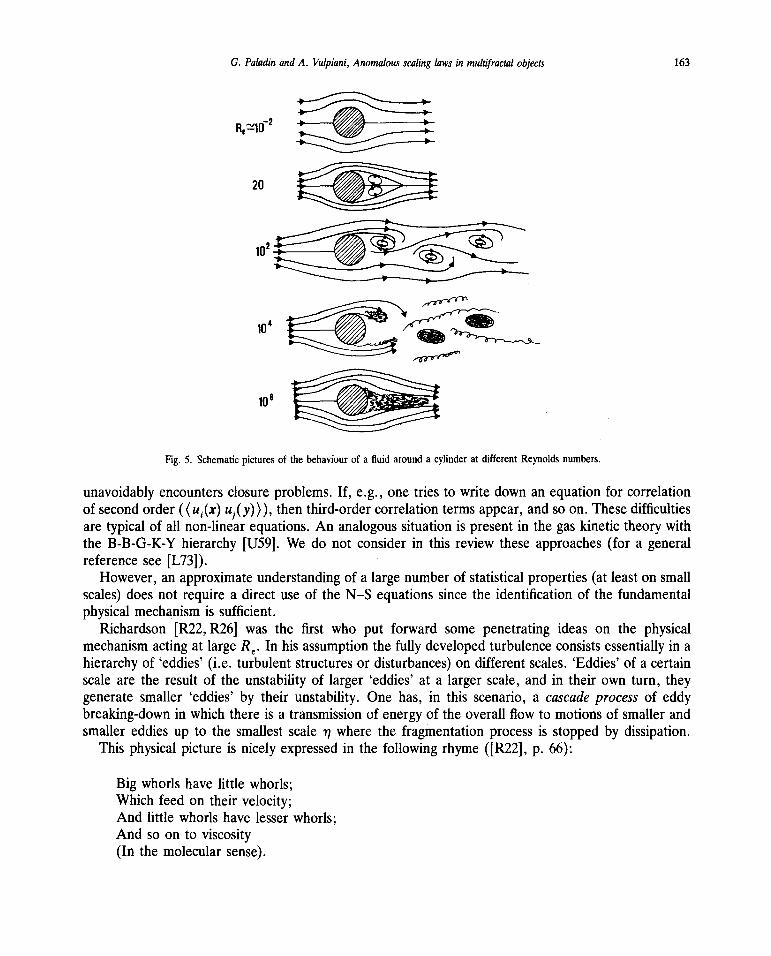
(i.e. roughly speakingthe evolution is regular and stable). On the contrary, at very large Reynoldsnumbersthere is a highly chaotic and irregular behaviour. The regime Re~ Rent is called fullydevelopedturbulencewhereRcrit is the valueof Re at which the onsetof turbulenceappears,i.e. thereis a transition from laminar to chaotic flow. We underlinethat for Re� Rent there are often onlytemporal chaosand highly spatialcoherentstructures.In the limit Re~ Rent the chaoticbehaviourinvolves fluctuationson a so small scaleof spaceandtime thatit seemspossibleonly a descriptioninterms of the staticalpropertiesof the flow. An ideaof the increasingchaoswith Re is given by fig. 5.
Turbulentflows are very commonin nature and they areof greatinterestin applicationsfor theirability to transfermomentumor heat.Other relevantpeculiaritiesof turbulentflows areunstabilityandunpredictability:a smallperturbationat a certaintime t
0 may rapidly leadto a strongdistortionof the(unperturbed)flow pattern [MY75].
In principle one could build up the statistical mechanicsof turbulence on the basis of theNavier—Stokes(N—S) equations:
1 1
lv.u=o p (2.1.1)+ initial and boundary conditions
whereu is thevelocity field, p the density,p thepressure,v the kineticviscosity andfan externalforce.Unfortunately,eachanalyticaltheory of turbulence,i.e. an approachwhich makesuseof eq. (2.1.1),
G. Paladin and A. Vulpiani, Anomalousscaling laws in multifractal objects 163
Re~iO2
20~
102
~
~
Fig. 5. Schematicpicturesof the behaviourof a fluid arounda cylinder at different Reynoldsnumbers.
unavoidablyencountersclosureproblems.If, e.g.,one triesto write down an equationfor correlationof secondorder((ui (x) u.(y))), thenthird-ordercorrelationtermsappear,andso on. Thesedifficultiesaretypical of all non-linearequations.An analogoussituationis presentin the gas kinetic theorywiththe B-B-G-K-Y hierarchy [U59]. We do not considerin this review theseapproaches(for a generalreferencesee [L73]).
However,an approximateunderstandingof a largenumberof statisticalproperties(at leaston smallscales)doesnot requirea direct useof the N—S equationssincethe identificationof the fundamentalphysicalmechanismis sufficient.
Richardson [R22,R26} was the first who put forward some penetratingideas on the physicalmechanismactingat largeRe. In his assumptionthe fully developedturbulence consistsessentiallyin ahierarchyof ‘eddies’ (i.e. turbulentstructuresor disturbances)on differentscales. ‘Eddies’ of acertainscaleare the resultof the unstability of larger ‘eddies’ at a larger scale,and in their own turn, theygeneratesmaller ‘eddies’ by their unstability. One has, in this scenario,a cascadeprocessof eddybreaking-downin which thereis a transmissionof energyof the overall flow to motions of smallerandsmaller eddiesup to the smallestscale ~ wherethe fragmentationprocessis stoppedby dissipation.
This physicalpicture is nicely expressedin the following rhyme ([R22], p. 66):
Big whorls havelittle whorls;Which feed on their velocity;And little whorls havelesserwhorls;And soon to viscosity(In the molecular sense).
164 G. Paladin and A. Vulpiani, Anomalousscaling laws in multifractal objects
Let us recall that theseconsiderationsarerelatedto the three-dimensionalcasesincein the bidimen-
sional situationsa quite different phenomenologyappears[PV86CIas discussedin section2.5.
2.2. Kolmogorov theory and the intermittencyproblem
The qualitative and generalideasof Richardsonhavebeenfurther developedandformulatedin amorepreciselanguageby Kolmogorov [K41].
Kolmogorov madean addition to the assumptionson the cascadeprocessby noting that, becauseofthe chaoticnatureof the energytransferamongthe eddies,the orientingeffectof the meanflow mustbe weakenedwith eachbreakingdown. Consequentlyit is naturalto expectthatat spatialscalesmuchsmaller than the externallength L (i.e. the typical length of the meanflow) and time scalesmuchsmallerthanthetypical time of the meanflow, the velocity fluctuationsarehomogeneous,isotropicandquasi-steady.At sufficiently small-scalethe turbulenceis thuscharacterizedby the meanflux of energy~ (from the overall flow to thesmallesteddy) andby thedissipation.Moreover,if the scalelength is nottoo smallit is naturalto assumethat the viscosityplaysno role, becausethedissipationtermin the N—Sequationsis negligible.
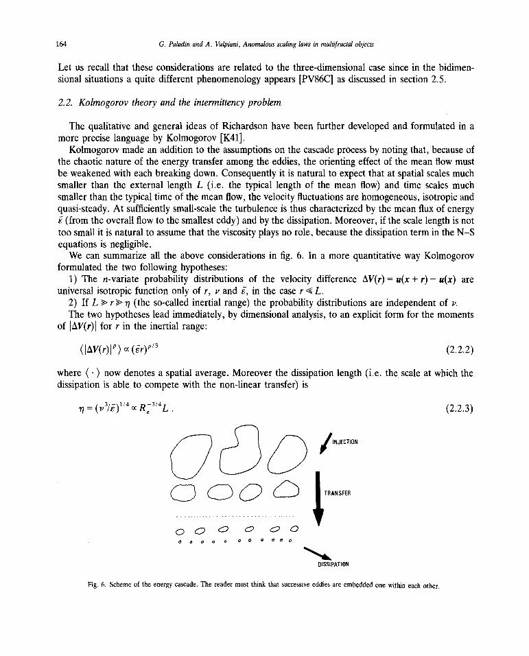
We can summarizeall the aboveconsiderationsin fig. 6. In a more quantitativeway Kolmogorovformulatedthe two following hypotheses:
1) The n-variate probability distributions of the velocity difference i~V(r)= u(x + r) — u(x) areuniversalisotropicfunctiononly of r, v and ~, in the case r ~ L.
2) If L ~ r ~‘ ~j (the so-calledinertial range) the probability distributionsareindependentof i.’.
The two hypothesesleadimmediately,by dimensionalanalysis,to anexplicit form for the momentsof ~V(r)~for r in the inertial range:
(4V(r)V) cc(~r)”~ (2.2.2)
where (~) now denotesa spatialaverage.Moreover the dissipationlength(i.e. the scaleat which thedissipationis able to competewith the non-lineartransfer) is
= (3/)1/4 R~31~L. (2.2.3)
0~Q ~ TRANSFER
Q ~7O
o a 0 0 0 0 0 0 000
D)SS)PAT)ON
Fig. 6. Schemeof theenergycascade.The readermust think that successiveeddiesareembeddedone within eachother.
G. Paladin and A. Vulpiani,Anomalousscaling laws in multifractal objects 165
Independentlyalso Onsager[045, 049] obtainedthe sameresultsas Kolmogorov.Let us stressthat the basic assumptionin the K4i theory is that ~ should be the only relevant
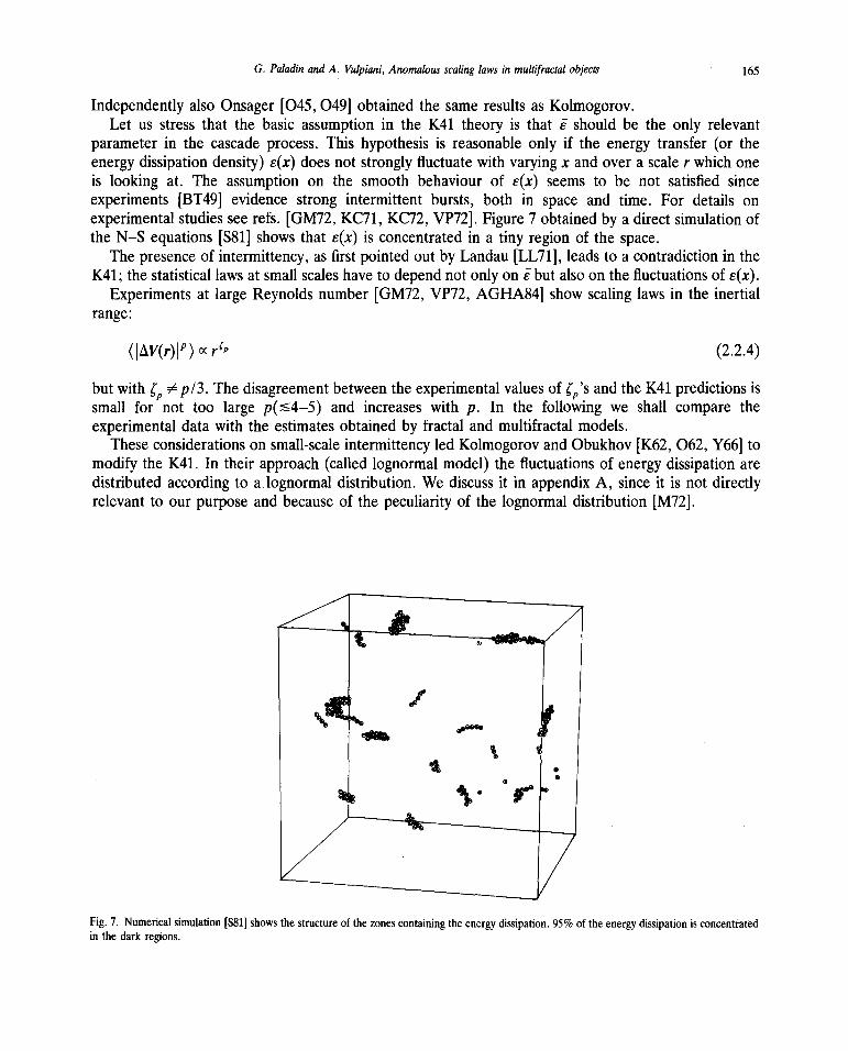
parameterin the cascadeprocess.This hypothesisis reasonableonly if the energytransfer(or theenergydissipationdensity) s(x) doesnot stronglyfluctuatewith varying x andoverascaler which oneis looking at. The assumptionon the smooth behaviour of s(x) seemsto be not satisfied sinceexperiments [BT49] evidence strong intermittent bursts, both in space and time. For details onexperimentalstudiesseerefs. [GM72,KC71, KC72, VP72]. Figure7 obtainedby adirect simulationofthe N—S equations[S81]showsthat e(x) is concentratedin a tiny region of the space.
Thepresenceof intermittency,as first pointedout by Landau[LL71], leadsto a contradictionin theK41; the statisticallaws at smallscaleshaveto dependnot only on ~but alsoon the fluctuationsof r(x).
Experimentsat large Reynoldsnumber[GM72, VP72, AGHA84] show scalinglaws in the inertialrange:
(I~V(r)V) ~ (2.2.4)
but with ~ ~ p13. Thedisagreementbetweentheexperimentalvaluesof ~‘s andthe K41 predictionsissmall for not too large p(~4—5)and increaseswith p. In the following we shall comparetheexperimentaldata with the estimatesobtainedby fractal andmultifractal models.
Theseconsiderationson small-scaleintermittencyled Kolmogorov andObukhov[K62,062, Y66] tomodify the K41. In their approach(called lognormalmodel) the fluctuationsof energydissipationaredistributed accordingto alognormaldistribution. We discussit in appendixA, sinceit is not directlyrelevantto our purposeandbecauseof the peculiarity of the lognormal distribution[M72].
a
/
S
S
Fig. 7. Numericalsimulation $81jshowsthestructureof thezonescontainingtheenergydissipation.95% of theenergydissipationis concentratedin the dark regions.
166 G. Paladin and A. Vulpiani, Anomalousscaling laws in multifractalobjects
2.3. Fractal and multifractal modelsfor intermittency
The K41 theoryassumesthat eachpoint x of the fluid hasthe same‘singularity’ structure:
~V1(r)csrh, h—i. (2.3.1)
It is easyto seethat (2.3.1) is equivalentto assumethats(x) is smoothlydistributedin a regionof R3.
Let usdefine the eddyturn-overtime and the kinetic energyper unit massat scaler:
1(r) —~rI~V(r) (2.3.2)
E(r)—i~V(r)2. (2.3.3)
The transferrate of energyper unit massfrom the eddy at scaler to smaller eddiesis thengiven by
~(r) = E(r)It(r) -= ~V(r)3Ir . (2.3.4)
Since s~(r)= (1 1r3) .fA(r) r(y) d3y (A~(r)is a cubeof edger aroundx), one hasby (2.3.4)and (2.3.1)
J r(y)d3y~r~.A~(r)
A simple way to modify the K4i consistsin assumingthat the active turbulent structurescover ahomogeneousfractal S (with DF <3) on which e(x) is uniformly distributed.
Let us remark that in turbulencewe do not usethe word fractal in the exact mathematicalsense.Indeedin the ‘true’ limit r —~ 0 becauseof the dissipationone probably finds no singular structures.r —*0 means r in the inertial range and the regions containinga large part of e(x) are a ‘physical’approximationof a fractal structure. In this approach(called absolutecurdling [M74] or f3-model[FSN78I)one replaces(2.3.5a)with
1 3 IrF ifxESj s(y)dyx~ 0 ifx~’S (2.3.5b)A~(r)
or in an equivalentway:
Irh ifxES
~V~(r)x10 ifx~’S (2.3.6)
with h = (DF — 2)13. Since at scaler thereis only a fraction
— numberof cubesof edger in S r~r — numberof cubesof edger in the fluid r3
occupiedby the ‘active’ eddies,we havein the inertial rangethe following behaviourfor the structurefunctions
G. Paladin andA. Vulpiani, Anomalousscaling laws in multifractalobjects 167
(Iz~V(r)V)c r~r31~= rip
D — 2 (2.3.7)( F ).P+(3DF)
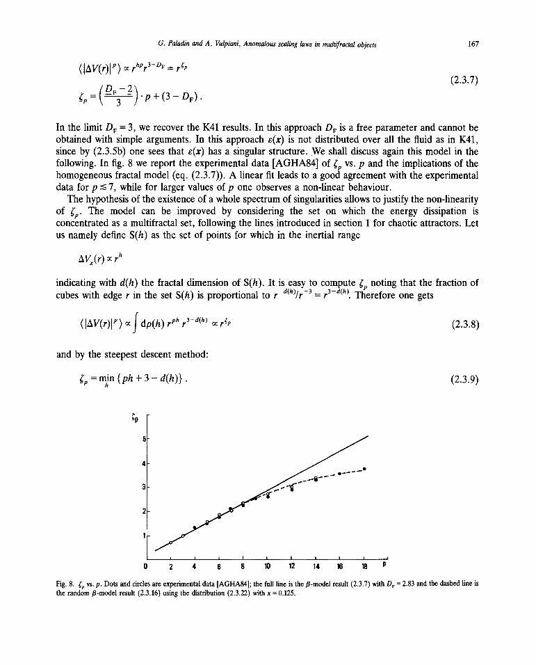
In the limit DF = 3, we recoverthe K41 results.In this approachDF is a free parameterandcannotbeobtainedwith simple arguments.In this approache(x) is not distributedover all the fluid as in K41,since by (2.3.5b)one seesthat e(x) hasa singularstructure.We shall discussagainthis model in thefollowing. In fig. 8 we report the experimentaldata [AGHA84] of vs. p andthe implicationsof thehomogeneousfractal model (eq. (2.3.7)).A linear fit leadsto agood agreementwith the experimentaldatafor p ~ 7, while for largervalues of p oneobservesa non-linearbehaviour.
Thehypothesisof the existenceof a wholespectrumof singularitiesallows to justify thenon-linearityof ~,. The model can be improved by considering the set on which the energy dissipation isconcentratedas amultifractalset, following the lines introducedin section1 for chaoticattractors.Letusnamely defineS(h) as the setof points for which in the inertial range
indicating with d(h) the fractal dimensionof S(h). It is easyto compute~ noting that the fractionofcubeswith edger in the setS(h) is proportionalto r _d~Ir~ = r3 d~• Thereforeonegets
(~V(r)j~)f dp(h) rPh r3~ ~ (2.3.8)
and by the steepestdescentmethod:
~~=min{ph+3—d(h)}. (2.3.9)
Fig. 8. vs. p. Dots andcirclesareexperimentaldata[AGHA84]; thefull line is thea-modelresult(2.3.7)with DF = 2.83 andthedashedline istherandom$-model result (2.3.16)using the distribution(2.3.22)with x = 0.125.
168 G. Paladin and A. Vulpiani, Anomalousscaling laws in multifracial objects
Equation(2.3.9)showsthat at a givenvalueof p, ~, dependson aparticularvalueof h. Hencethekindof instabilitiesneededto set up the setsS(h) arepicked up by differentmoments.
We haveworked out the multifractal approachin termsof singularitiesof L~V~(r) only becausein theliterature of turbulence the moments (I~V(r)i”) are usually involved. However it is simple toemphasizethe explicit correspondencewith chaoticattractors.Let usnote that
J r(y)dy~r3~(r) ~r3~2 (2.3.10)
A~(r)
so that the analoguesof the exponenta andf(a) are 3h + 2 and d(3h + 2).The homogeneousfractal caseis the limit of the multifractal one when d(h) is defined only for
h=(DF—2)13 andd(h)=DF.Up to now we haveremainedat a rather descriptivelevel in the problemof intermittency. d(h)
containsall the relevantfeatures,but cannotbe obtainedby a first principle calculationbasedon theN—S equationsingularities.
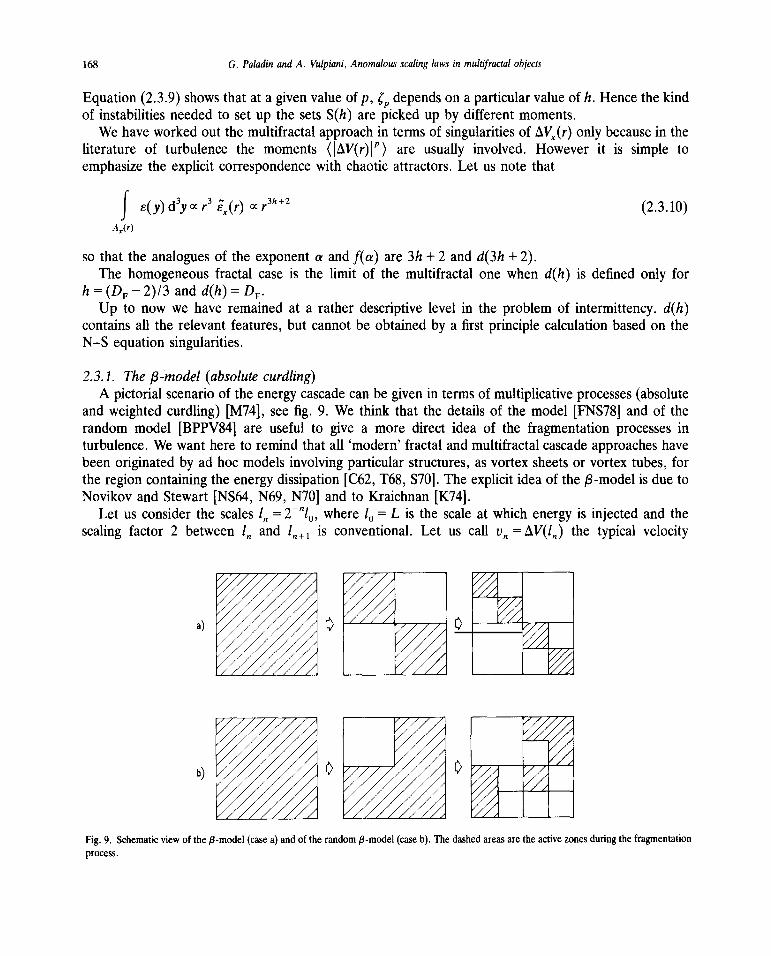
2.3.1. The p-model(absolutecurdling)A pictorial scenarioof theenergycascadecan be givenin termsof multiplicative processes(absolute
and weightedcurdling) [M74], see fig. 9. We think that the detailsof the model [FNS78]and of therandom model [BPPV84] are useful to give a more direct idea of the fragmentationprocessesinturbulence.We want hereto remindthat all ‘modern’ fractal andmultifractalcascadeapproacheshavebeenoriginatedby ad hocmodelsinvolving particular structures,as vortex sheetsor vortex tubes,forthe region containingthe energydissipation[C62,T68, S70]. Theexplicit ideaof the f3 -modelis duetoNovikov and Stewart [NS64,N69, N70] and to Kraichnan[K74].
Let us considerthe scales1,, = 2 ~ where l~= L is the scaleat which energyis injectedand thescaling factor 2 betweenIn and 1,,~ is conventional. Let us call Vn = ~V(l~)the typical velocity
—~ N
b)Ø~Jj~
Fig. 9. Schematicview of the13 -model(casea) andof therandomfl-model(caseb). Thedashedareasaretheactive zonesduringthefragmentationprocess.
G. Paladin andA. Vulpiani, Anomalousscaling laws in multifractalobjects 169
differenceacrossa distanceI,, in an activeeddy. In orderto takeinto accountthe intermittencyFrischet al. [FSN78]introducedthe coefficient /3 =
2DF equalto the fraction betweenthe volume of thedaughtereddiesat scalei,~+ andthe volume of the mothereddyat scale1,. The transferenergyfromthe eddyat scale in to that at scale ln+1 is
En ~ U~Iln
Sincethe energytransferrate is constantin the cascadeprocessone has
Sn = /3~n+1’ v~II~/3 v~+1Ii~+1. (2.3.11)
Iterating (2.3.11) one thenobtains
l3(I~II~)F_3~3 (2.3.12)
i.e. eq. (2.3.6) with h = (DF — 2)13.In the previousmodeloneessentiallyhasa two-valuedmultiplicative process:eacheddy at scaleI,, is
divided into eddies of scale1n + 1’ in such a way that the energy transfer for a fraction /3 of eddies
increasesby a factor 1//3 while it becomeszero for the other ones.
2.3.2. The random /3-model(weightedcurdling)Let usgeneralizethe p-model. We namely assumethatat scale1n thereareNn active eddies,each
eddy In(k) (k labelsthe ‘mother’ eddyandk = 1,. . . Pin) generatesactiveeddiescoveringa fraction ofvolume 13,,+
1(k). Since the rate of energytransferis constantamongmother and daughters,we get:
Un(k)3/in = /3n+i(k)Vn+i(k)311n+i . (2.3.13)
The iteration (2.3.13) of On gives an eddy generatedby a particular ‘history’ of fragmentations
Vn i~3(fJ13~)h/3~ (2.3.14)
Let us remarkthat the fraction of volume occupiedby an eddygeneratedby [13k,. .. /3~]is 1~1 /3,, 50
from eq. (2.3.14) it follows -(~v(l~)I~)i’~f fi d/3, pdl~3)p(p
1,.../3,,). (2.3.15)
Assumingno correlationamongdifferent stepsof the fragmentation,i.e. P(~ fan) = P( /3,),oneobtainsfor -
~ =p/3 —ln2{/3~”3~} (2.3.16)
where{ } standsfor the averageoverthe distributionP(/3). If /3, is a constant(2(DF
3)) onerecovers
170 G. Paladin andA. Vulpiani, Anomalousscaling laws in multifracial objects
the results of the /3-model. The knowledge of the probability distribution P( /3) is related to theunderstandingof thenatureof the N—S equationsingularities.Howeverthis problemis far to besolvedat present.The fractal objectgeneratedby therandom/3-model(ormoregenerala multifractalobject)hasno more globaldilatation invariantproperties;evenif, onecan still computethe fractal dimensionDF as:
(2.3.17)
whereN,, is thenumberof activeeddiesat thenth stepof the fragmentationand(~)is an averageover
an ensembleof cascades.It is easyto show that
DF = 3 — ~o (2.3.18)
which in the random/3-modelis given by:
DF = 3 + 1n2{13}. (2.3.19)
Moreoverthe analogueof d2 is D * definedby:
D*=i+~6 (2.3.20)
andin termsof the random/3-model
D*=3_ln2{/3~} . (2.3.21)
Let us recall that D * is relatedto the scalingof energydissipationdensity correlation[FSN78],
(s(x+ r) 5(x)) cc r3~
and that in the experimentalliterature the fractal dimensionis usually estimatedby D * evenif ingeneralDF > D ~ DF = D * actuallyholds only for homogeneousfractals.
We haveperformeda simple fit of the experimentaldatachoosingfor P( /3) the form
P(/3)=x~(/3-0.5)+(1-x)~(/3-1); (2.3.22)
the value x = 0.125 gives good agreementwith the experimentaldata (see fig. 8). -There is no deepreasonto choosethe form (2.3.22);we havesimply followedsomephenomenologicalideasconsideringtwo possible kinds of fragmentation:an activeeddy can generateeither vorticity sheets(/3 = 0.5) orspacefilling Kolmogorov-like eddies (/3 = 1). With the fit (2.3.22)we get DF = 2.91 and D* = 2.83,with a small but significant difference.There exist somephysical argumentsto give a bound to thevaluesof h. In thesetS(h) thelocal Reynoldsnumberat scaler is Re(r, h) = r’ r”Iv cc ~ Thereforeinorderto stop the turbulent cascadeonemust requirethat R~(r,h) decreaseswith r implying h> —1.Let us notehowever,that it is reasonableto assumeh � 0 becausefor negativeh onecouldhavepointsfor which ~V~(r)Iincreaseswhen r decreasesand this seems quite unrealistic. Note that in thedistribution (2.3.22)we havetakenhmjn = 0 (correspondingto /3mm = ~).
G. Paladin and A. Vulpiani, Anomalousscaling laws in multifractal objects 171
Mandeibrot [M76b]conjectured,using Taylor’s frozen turbulenceassumption[T38],that fractalstructurewith a fractal dimension <2 cannotbe detectedin a realexperiment.
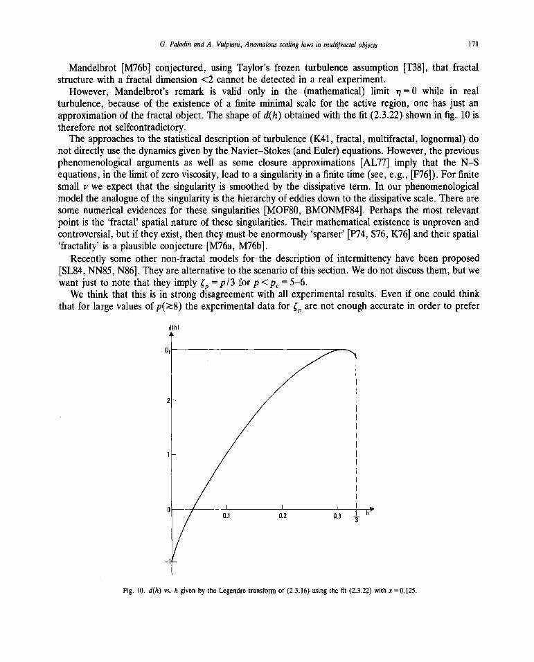
However, Mandelbrot’s remark is valid only in the (mathematical)limit ~ = 0 while in realturbulence,becauseof the existenceof a finite minimal scale for the active region, one hasjust anapproximationof the fractal object. The shapeof d(h) obtainedwith the fit (2.3.22)shownin fig. 10 isthereforenot selfcontradictory.
The approachesto thestatisticaldescriptionof turbulence(K41, fractal,multifractal, lognormal)donot directlyusethedynamicsgiven by the Navier—Stokes(andEuler)equations.However,thepreviousphenomenologicalargumentsas well as some closure approximations[AL77] imply that the N—Sequations,in the limit of zero viscosity,leadto a singularity in a finite time (see,e.g.,[F76J).For finitesmall v we expect that the singularity is smoothedby the dissipativeterm. In our phenomenologicalmodel theanalogueof thesingularity is thehierarchyof eddiesdown to thedissipativescale.Therearesome numericalevidencesfor thesesingularities[MOF8O,BMONMF84]. Perhapsthe most relevantpoint is the ‘fractal’ spatialnatureof thesesingularities.Their mathematicalexistenceis unprovenandcontroversial,but if they exist, thenthey mustbeenormously‘sparser’[P74,S76,K76] andtheir spatial‘fractality’ is a plausibleconjecture[M76a,M76b].
Recently someother non-fractal modelsfor the descriptionof intermittencyhavebeen proposed[SL84,NN85, N86]. Theyarealternativeto thescenarioof this section.Wedo not discussthem,butwewant just to note that they imply ~ = p13 for P<p~= 5—6.
We think that this is in strongdisagreementwith all experimentalresults.Even if one could thinkthat for largevaluesofp(~8)the experimentaldatafor arenot enoughaccuratein order to prefer
d(h)
2~ I
0.1 0.2 0.3 -~-
Fig. 10. d(h) vs. h given by the Legendretransformof (2.3.16)usingthe fit (2.3.22)with x = 0.125.
172 G. Paladin andA. Vulpiani, Anomalousscaling laws in multifractal objects
definitively a model or another,all the recent experimentsneverthelessgive values for ~ and ~
respectivelylargerandsmallerthan 2/3 and 4/3 obtainedby the K41 (e.g. ~2 = 0.70±0.01).
2.4. Remarksand consequencesofmultifractaiiiy in turbulence
The conceptof ‘multifractal’ is relatedto the propertiesof thedistributionof ‘mass’ (in turbulencethedensityof energydissipation,in a chaoticsystemthedensityof pointson theattractor)andnot to‘geometrical’ properties[M86,BPPV86].
For examplethereis no anomalousscaling law for the numberof activeeddiesN,,:
N’7 (N)’7 cc çDF~ (2.4.1)
where (.) means the averageof an ensemble of cascades.Equation (2.4.1) is a quite trivialconsequenceof the law of largenumbers.For sakeof completenesswe considerthe random/3-modelofsection2.3.2 where the numberof active eddiesat scale in is
N~=23n{IB~ (2.4.2)
with
B~=’ ~ /3~(k). (2.4.3)k=1
In the limit of largen (i.e. )V~~‘ 1) one has(largenumbertheorem):
the probability distribution of N~has thereforea very narrow peak around 2~”{ ~ n = DF so that(2.4.1) holds. Equation (2.4.1) can easily be proved for positive integer values of q by directcomputation[BPPV86].
2.4.1. Irrelevanceof multifractalityfor relative diffusionLet us now showwhy the multifractalstructureis not relevantfor therelative diffusion of particle
pairs [CPV87].Indeed,the growthof themomentsof the relativedistanceRbetweena pairof particlesscaleswith
time as:
~
12q v(q) (2~4.4)
(~ is nowan averageover a largenumberof pairs).We foundthat for eachq, v(q) = v and v is only
relatedto the exponent~:(2.4.5)
G. Paladin andA. Vulpiani, Anomalousscaling laws in multifractal objects 173
Let us consider M ~ 1 pairs of particlesat positionsr~’~and ~~2) (i = 1,. . . M). The interparticiedistanceis R, = (r~’~— r~2~)and the relativevelocity bV~= u(r~)— u(r~2’)= (dldt)R
1.Let us computethe time derivativeof R
2:
~R2=2lim~ >~V~(R1).R~
=2lim~ >~V,(R~)R~cosO, (2.4.6)
where0, is the anglebetweenR, and~V,(R1).In the caseof isotropic turbulencethe relative positionsandvelocitiesareuncorrelated[MY75 section24, C69, 070a],moreovercos0 is positive anddoesnotdependon R [C69,070]. Thereforethis one has
dR2Idt= 2 (~~) ~V(R)R. (2.4.7)
In order to computeM’ . ~ W,(R~)R,= M7(R) Rwe grouptogetherall then(a) pairswith thesame
valueR(a) of the interparticledistancein sucha way that oneobtains:
~ W,.(R,)R, = E [—~—-~ ~Vk] R(a). (2.4.8)i=1 a n(a)
The sum ~,, is over the -set of different valuesof R(a) and Ek is over the n(a) pairswith Rk = R(a).Note that for large M (and n(a))
~ 8V~-~(~V(R(a))~)ccR(a)’1 (2.4.9)
n(a) k
therefore
dR2IdtccRl+u1. (2.4.10)
It is trivial to repeatthe samecomputationsfor R2’7:
dR2’7/dtccR2’7~”1. (2.4.11)
Now it is easyto see that v(q), as definedin (2.4.4), mustbe constant.In fact by (2.4.11)and(2.4.1)onehas
f2q—l+~1\
2qv(q)—1=(2q—i+~1)’v~ 2
moreoverv(q) doesnot increasewhen q increases[F71],thereforeoneobtains:
r.’(q)=v1I(1—~1), Vq.
Let us remarkthat the multifractal structureinducesonly a (slight) correctionto the Richardsonlaw
174 G. Paladin and A. Vulpiani, Anomalousscaling laws in multifractal objects
= ~[R26]and in the diffusion processthereis no anomalousscaling.The scalinglaws (2.4.4,2.4.5)are parametrizedby a single exponent~ the sameresult holds for a homogeneousfractal [HP83b](with ~ = (7 — 2DF)/3) or a multifractal.
2.4.2. Theproblemof the numberof degreesoffreedomIt is clear thatasatisfactorydescriptionof turbulentfluids needsaresolutionup to scaleof the same
orderof thedissipativeKolmogorovlength~qat which themolecularfriction is ableto competewith thenon-lineartransfer.Onehas:
= (3/)1/4 (2.4.12)
where s is the rate of the energydissipationfor unit massandtime (assumedto be constantin K41).If L is the systemcharacteristiclength at which the external energyinput is pumpedthen the
adimensionalratio Re = (sL4)1/3/v is theReynoldsnumber.The numberof grid points for unit volume
necessaryto obtain a resolutionup to i~ is thus
N(Re)-= (LI’q)3 cc R’4. (2.4.13)
This argument(due to Landauand Lifschitz [LL71])hides the centralassumptionthat all the fluid is‘active’, i.e. that the energydissipationdensity field is smoothly distributedon a three-dimensionalregion.
Kraichnan[K85]hasrepeatedthe Landau—Lifschitzargumentby making the hypothesisthat theenergydissipations(x) is concentratedon a homogeneousfractal with non-integerdimensionDF <3.The dissipationscale ~j can be now determinedby imposingthat the Reynoldsnumberrelatedto aneddyof length scale1 is of order one:
?im~V(’1i)lv-.-O(i). (2.4.14)
This is equivalentto requirethat thedissipative(linear) termof the N—S equationis ableto competewith the non-lineartransferterm.
Insertingeq. (2.3.6)in eq. (2.4.14)we obtain:
(2.4.15)
It follows that:
N(Re) (LI~)~cc RF/+D~ . (2.4.16)
Let us remark that someother variablesarealso necessaryfor describingthe non-activeregionsofthe fluid but their number doesnot dependon Re~If the /3-model assumptionswere correct, eq.(2.4.16)would give (in principle) the scaling law for N(Re).
The numberof degreesof freedomnecessaryfor describingthe multifractalof turbulencemustbedefinedwith muchmorecarefulness[PV87a].In fact, for eachsingularity h a different dissipativelengthi1(h) is pickedup by condition(2.4.15): ~(h)ccR~.
Sincethenumberof eddiesat scale1 with singularityh is proportionalto I - d(h) onededucesthat the
G. Paladin andA. Vulpiani, Anomalousscaling laws in multifractal objects 175
numberof grid points which haveto be consideredfor resolvingthe setS(h) is:
Nh(Re) (LIi~(h))~cc ~ (2.4.17)
We thus get the total numberof degreesof freedomby integrating(2.4.17)over
N(Re)= f dp(h)Nh(Re) R~ (2.4.18)
where ö canbe estimatedby the steepestdescentmethodin the limit of largeRe
8 = max[d(h)/(l + h)]. (2.4.19)
A fit of the experimentaldata [AGHA84] gives the value 6 2.2 which is closeto the valuegiven byeq. (2.4.16).
The results(2.4.16)and(2.4.18,19) areneverthelessquitedifferentfrom aconceptualpoint of view.We muststressthat the estimate(2.4.18,19) hasjust a theoreticalrelevancesinceit is ratherdifficult
in acomputersimulationto locate the grid pointson the setsS(h) (which alsoevolvesin time). Indeedoneusually works with a fixed grid or with a pseudo-spectralmethod[P071].It follows that the onlyrelevantparameteris theminimal scale1mjn consideredwhich is boundedfrom below by thedissipativelength relatedto the strongestsingularity:
lmmn ?l(hmin)cc R +hmii,) (2.4.20)
The estimate1min = fl(’t2min) assuresthat all the setsS(h) (i.e. evenvery improbableevents)aretakeninto account.
The numberof equationswhich allows us to get such a fully accuratedescriptionis thus:
N (Llimjn)3 cc R~~~”m1f1). (2.4.21)
Equation (2.4.21) is in agreementwith rigorous bounds[R82, CFMT85]. On the other hand, if onedecidesto neglect the rare events a resolution 1 ~‘ ~ is sufficient; just the relevant featuresofturbulenceare reproducedloosing somedetails. In this case the numberof equationsis reducedto
N*~=(L/i)3
This scaleI can be estimatedby the dissipativelength ~(h) relatedto an effective singularity h.Let us define an ‘effective’ mass dimension D of the object on which the energydissipationis
concentrated,by:
h=(ñ—2)13.
Mandeibrot [M76b]has, e.g., assumedD = D1, the information dimension, and from the data
[AGHA84]one has D1 2.87. This assumptioncorrespondsto select a h = d~~Idpj~,30.29 and,roughly speaking,1 is thus the smallestscaleon which in averageactive eddiesare still present.
On theotherhand,someheuristicarguments(seesection2.3) aswell asthe fit of experimentaldatashownin fig. 10 indicatehmjn = 0. It follows that:
176 G. Paladin andA. Vulpiani, Anomalousscaling laws in multifractal objects
NccR~ and N*ccR3/()ccR23
Let us emphasizethat N~.is much greaterthanN* which is close to the estimateof the numberofdegreesof freedom obtained respectively in K41, in the /3-model and in the framework of themultifractal approach.
2.5. Two-dimensionalturbulence
Two-dimensionalfluids havea relevantinterest,apartfrom a mathematicalpoint of view, becausethey idealizegeophysicalphenomenain the atmosphere,oceansandmagnetosphereand area startingpoint for understandingthesephenomena(seefor a generalreview [KM8O]).
The motion of fluids in two dimensions has many remarkable regularity propertieswhich areessentiallydue to the fact that the vorticity of eachfluid elementis constantif viscosity and externalforcing areabsent.Forthis reason~ dependson viscosity andthereis no forwardenergycascade[077].
Nevertheless,quite reasonablearguments[K67, B69] allow to repeat a K41-like approachbyassumingthe meandissipationenstrophy~ = — (d / dt) ((rot u)2) as the relevantparameter(insteadof~) andthusa forwardcascadeof enstrophy(insteadof energy).Oneobtainsby dimensionalanalysis,inthe inertial range:
(IAV(r)V)ccr’P, =p (2.5.1)
andfor the energyspectrum
E(k) k3. (2.5.2)
There exist numericalevidencesfor an energyspectrumin strong disagreementwith (2.5.2), i.e.E(k)cc k0, a —4 to —6 [BLSB81, M84]. Some authorsarguedthat this differenceis related tointermittency[BLSB81].
Let usbriefly showthatin two-dimensionalturbulencea K41-like theory givesthe exactscalingfor(i.e. ~ =p) which is not affectedby the ‘intermittency’.
One could naively think that either the fractal or multifractal approachcan be repeatedfordescribingthe enstrophycascade.This is not true becausein the two-dimensionalEulerequation,asconsequenceof the vorticity conservationfor eachfluid particle, onecan prove [RS781:
~V(r)~<const.r Rn rI . (2.5.3)
The inequality (2.5.3) also holdsfor the N—S equationsso that
(2.5.4)
Moreover mustbe convex[F71Jand ~ = 3, in order to haveaconstantforwardenstrophycascade.All theseconstraintscompelus to concludethat:
(2.5.5)
which implies theapparentlysurprisingresult that the K4i-like theory prediction~ = p also holds inpresenceof intermittency.
It is easy to see that a two-dimensional/3-model (or random /3-model),whenever/3,, ~ 1 gives a
G. Paladin and A. Vulpiani, Anomalousscaling laws in multifractal objects 177
wrong result for the enstrophycascade.Indeedif we repeatthe considerationsof section2.3 for the
three-dimensionalcaseimposinga constantenstrophytransferrate we get, insteadof eq. (2.3.13):
v,,(k)3/l~= f3,,~
1(k)v~~1/1~~1. (2.5.6)
This equationgives a convexfunction ~, (if f3~(k) ~ 1). The apparitionof singularitiesin the velocityfield follows by the Bernoulliannatureof the fragmentationprocess(/3,, is independentby /3,,-1).
However, the random/3-modelcan be modified assumingthat
/3n+1 =1 if (v~I1,,)~> ~max~ (2.5.7)
Equation(2.5.7)correspondsin somesenseto a “Markovian” assumptionin the fragmentationmodelbecausethe stepsof the cascadeare no longer independent.The constraint(2.5.3) is now satisfiedinthis Markovian random/3-model,but the enstrophyis concentratedin regionswith fractal dimensionequalto 2, which cover a non-decreasingareafor decreasingscalelength.
Let us notethat unlike the three-dimensionalcase,wecan reachno conclusionson the shapeof E(k)from ~. The naivedimensionalcounting gives E(k)cc k- with a = 1 +
This is wrong if ‘2 � 2 [BBS84Iand one can just derive from the bound(2.5.3):
a � 3. (2.5.8)
Therefore,neitherthe avaluenor the structurefunctions(since~, = p) give us informationabout the‘intermittency’ in two-dimensionalturbulence. Numerical experiments[BPPSV86Jconfirm that thefragmentationis space-fillingon the small scales(but largerthan the viscosity dissipationones).Theintermittency should be regardedas a somewhat“macroscopic” phenomenarelated to coherentstructures.
The enstrophycascadeindeedseemsto be inhibited in some highly organizedstructureswhichdominatethe energyspectrum.Moreover the turbulentfield seemsto be decomposedin two parts:abackgroundwith an energyspectrumk
3 in the inertial rangeanda finite numberof vortices(coherentstructures)which advectthe backgroundfield.
3. Temporal intermittency in chaotic dynamical systems
3.1. General remarks
One of the relevantfeaturesof chaotic systemsconsistsin their unpredictability.Essentiallyoneobservesthatnearbytrajectoriesdivergeexponentiallyin time. However, thereexist time variationsofthe ‘chaoticity’ which appearin all genericalsituationsand consequentlythe meanexponentialgrowthof the uncertaintyon the initial statedoesnot exhaustall the typical behaviours.
One can, e.g., observea regularmotion in phasespacefor long times, interruptedby randomlydistributed bursts of strong chaoticity. This phenomenon,called temporal intermittency, plays animportant role. For example intermittency has beenshown to be [PM8O]one of the fundamentalmechanismsfor the transition to turbulence.
178 G. Paladin andA. Vulpiani, Anomalousscaling laws in multifractalobjects
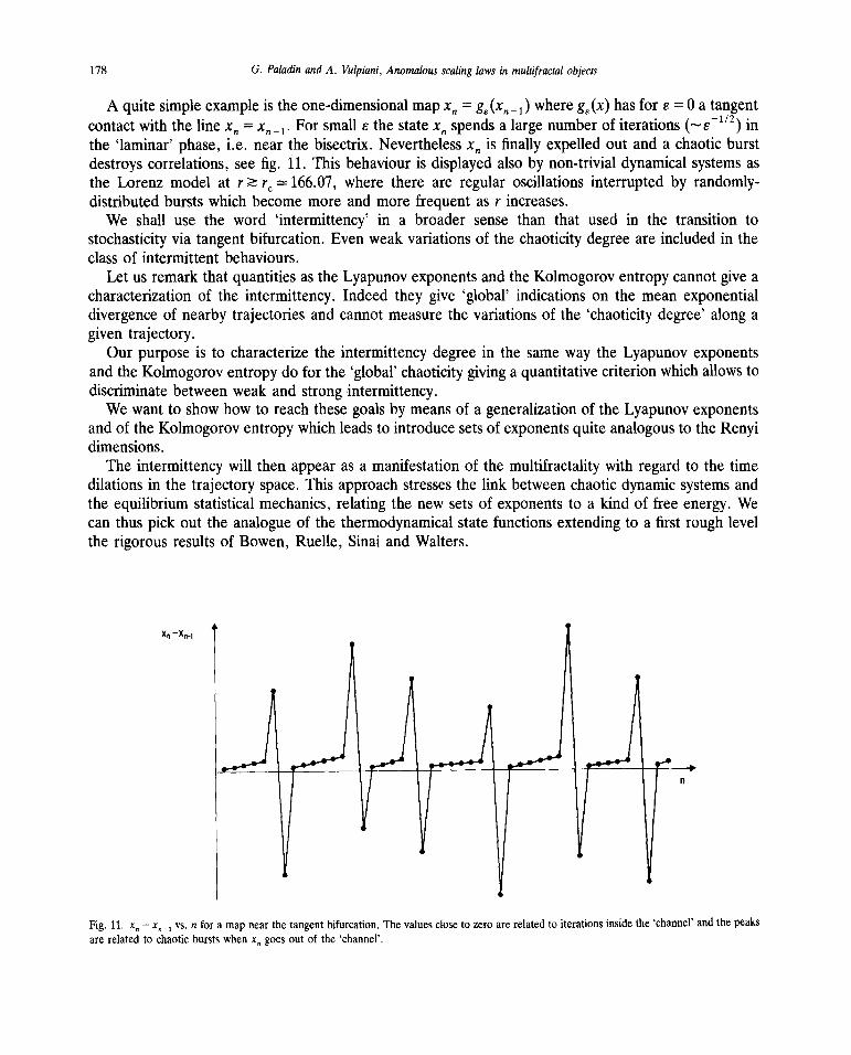
A quitesimpleexampleis the one-dimensionalmapx,, = g~(x,,-1) whereg6 (x) hasfor s = 0 a tangentcontactwith the line x,, = Xn .~. For small s the statex, spendsa largenumberof iterations(~~~1/2) inthe ‘laminar’ phase,i.e. nearthe bisectrix.Neverthelessx,, is finally expelledout and a chaoticburstdestroyscorrelations,see fig. 11. This behaviouris displayedalsoby non-trivial dynamicalsystemsasthe Lorenz model at r ~ r~ 166.07, wherethere are regular oscillations interruptedby randomly-distributedburstswhich becomemoreandmorefrequentas r increases.
We shall use the word ‘intermittency’ in a broader sensethan that used in the transition tostochasticityvia tangentbifurcation. Evenweakvariationsof the chaoticitydegreeareincludedin theclassof intermittentbehaviours.
Let usremarkthatquantitiesas the Lyapunovexponentsandthe Kolmogorov entropycannotgive acharacterizationof the intermittency. Indeedthey give ‘global’ indicationson the meanexponentialdivergenceof nearbytrajectoriesandcannotmeasurethe variationsof the ‘chaoticity degree’along agiven trajectory.
Our purposeis to characterizethe intermittencydegreein the sameway the Lyapunovexponentsandthe Kolmogorov entropydo for the ‘global’ chaoticitygiving aquantitativecriterion whichallows todiscriminatebetweenweakand strong-intermittency.
We want to showhowto reachthesegoalsby meansof a generalizationof the Lyapunovexponentsandof the Kolmogorov entropywhich leadsto introducesetsof exponentsquite analogousto the Renyidimensions.
The intermittencywill thenappearas a manifestationof the multifractality with regardto the timedilations in the trajectoryspace.This approachstressesthe link betweenchaoticdynamicsystemsandthe equilibrium statisticalmechanics,relatingthe new setsof exponentsto a kind of free energy. Wecan thuspick out the analogueof the thermodynamicalstatefunctionsextendingto a first roughlevelthe rigorous resultsof Bowen,Ruelle, Sinai andWalters.
xn —xi,~i
n
Fig. 11. x~— vs. n for a mapnearthetangentbifurcation.The valuescloseto zeroarerelatedto iterationsinside the ‘channel’ andthepeaksare relatedto chaoticburstswhenx~goesout of the channel’.
G. Paladin and A. Vulpiani, Anomalousscalinglaws in multifractalobjects 179
3.2. GeneralizedLyapunovexponents
A practical tool for characterizingthe global degreeof chaos in dynamical systemsconsistsinconsidering the set of Lyapunov exponentsbecausethey can be computed by means of simplealgorithms [BGS76,BGGS8O]. Moreover they are linked to other stochasticity indicators like theKolmogorov entropy [P77]and the information dimension[KY78].
Let us define the spectrumof the Lyapunov exponentsA1 � A2 � . � A~of the flow T: R’~—s’R’~generatedby the setof differentialequationsi = 1(x) by consideringthe linear evolutionof the tangentvector~:
t~=~ J~1 (3.2.1)
where is the matrix af,IdXJ~X(~).Onecanintroducethe Lyapunovexponentsalsofor adiscretemapx(n) = g(x(n — 1)) by considering
the correspondingevolutionfor ~(n):
A~1(n-1)~~(n-1)with A,1(n)= ~9g~/oxJJ~(,,).Oseledec[068] provedthat for almostall initial conditionsx(0) thereis abasis {i,} in R’~suchthat:
~(t) =±J~(°)Ic~1, exp(A1t) (3.2.2)
for largeenoughtimes.Roughlyspeaking,(3.2.2) tells us that in the phasespacea sphereof radius s and centrex(0) is
deformedwith time into an ‘ellipsoid’ of semi-axess~(t)= sexp(A,t) directedalongthe 1, vectors.In the next section we shall show that the Oseledectheorem correspondsto the existenceof a
thermodynamiclimit of infinite volume in a statisticalmechanicslanguage.The positive maximal Lyapunov exponent A1 measuresthe growing of an error on the initial
- condition knowledge.A small incertitude6x(0) is exponentiallyamplified alongI~with characteristictime A~.To be more specific eq. (3.2.2) implies that for A1 > A2:
&r(t) — &x(0)~ê1 exp(A1t)[1+ O(exp{—(A1 —
This relationleadsus to introducethe responseR to a perturbationin x(r) after a time t by the errorgrowth rate:
Rr(t)_= IIC(t+ r)~I/J~~(i)JlH~x(t+ T)I/16X(T)J . (3.2.3)
The maximalLyapunovexponentcan be definedby averagingthe logarithmof the responseover thepossibleinitial conditionsalong the trajectory:
180 G. Paladin and A. Vulpiani, Anomalousscaling laws in multifracial objects
= lim (in R(t)) (3.2.4)r+T
where (.) denotes~ (lIT) $~ dt.In the same way we can define the other Lyapunov exponentsby the divergenceof a small
n-dimensionalpoint volume in phasespace.Let us namelyconsidern different tangentvectors~ ~ ~.(n)The rate of an n-dimensional
volume is thenmeasuredby an n orderresponse~ definedas:
~ — 1 ~(l)~ + T) A ~~2~(t + r) A A ~~(t + r)M (3 2 5)(t) - C~()A ~(2)() A A
where A denotesthe vectorialproduct.The sum of the first n Lyapunovexponentsis [BGGS8O]:
A1 = lim (ln R~”~(t)). (3.2.6)
Let usalso remarkthat, in the caseof continuousflow, at leastoneof the Lyapunovexponentshastobe zero since ~(t) cannotgrow exponentiallyin time aiong the direction tangentto the flow.
3.2.1. Characterizationof intermittencyThe Lyapunov exponentsdo not describe the degreeof intermittency becauseof their global
character. Equation (3.2.4), e.g., defines the averageof the characteristictime scale on whichcorrelationsare lost but it does not give any further information about the fluctuationsaroundthisaverage.Indeed,we muststill consideranon-uniformdistributionin timeof the ‘chaoticity degree’,i.e.of the responseR.
The reconstructionof the probability distribution of R can be achievedby the analysisof themoments(R~).
Let us thereforeintroducethe function [F83,BPPV85]:
.1L(q) = lim -~ ln(R(t)~). (3.2.7)
L(q) is called generalizedLyapunovexponent(of orderq) since:
A1 =dLIdq~q...0 (3.2.8)
and in the absenceof fluctuations
L(q) = A1q (3.2.9)
while in the generalcaseL(q) is concavein q [F71].The deviationsfrom this linear law give a first rough indication on the intermittencydegreein the
sameway that the set of ~q)’s is used to characterizethe spatial inhomogeneitywith regardto thepoint density(seesection1.1).
G. Paladin and A. Vulpiani, Anomalousscaling laws in multifractal objects 181
Equation(3.2.9) correspondsto long rangecorrelationswhich inhibit fluctuations.However if thecorrelationsare weak enough the responseat time Nm~tcan be consideredas the product ofindependentrandomvariablesR, = R~+1.~~(iXt):
R~(t=Nat) = H R1(At). (3.2.10)
As consequenceof the central limit theorem, the probability distribution of R~is thereforewellapproximatedby the lognormal:
~(R) = 1 1/2 ~ exp{_ (ln R — Ait)2} (3.2.11)
(2i~tt) R 2~st
where js = ~ t’[(ln R(t)2) — (A1t)
2].If (3.2.11) is exact thenthe generalizedLyapunovexponentsare:
L(q) = A1q + ~j~q
2. (3.2.12)
It is thus natural to conjecturethat, in the general case,L( q) is boundedbetweenthe linear form(3.2.9) (strongcorrelations)and the parabolicone (3.2.12)(weak correlations).
Let ushoweverrecall that at largeq the momentsdeviatefrom (3.2.12)evenif the lognormal is agood approximationbecauseof the pathologiesof this distribution (seeappendixB).
In (3.2.11)the fluctuationsarefully characterizedby the secondcumulantj~and it is easyto showthat the value ~ IA~= 1 delimits the borderlinebetweenweak and strongintermittency. To be morespecific let us remark that~P(R)reachesits maximum for
R(t) = exp(A11(1 — ~IA1)). (3.2.13)
It follows that for large times:
R—*0 if ~aIA1>1 (3.2.14)
R—s.cc ifp.1A1’(l.
The equations(3.2.14)give, in the phasetransitionjargon,a meanfield resultand it is interestingtoanalysetheeffects of the corrections.For p.1A1<1 the fluctuationscan beneglectedata first level sincethey just slightly modify the characteristictime on which the ‘average’ responsediverges fromA~(1— 1slA1)~to A~
1.
On the contrary,the meanfield picturefully breaksdown for ~ IA1 > 1 whereit predictsa ‘laminar’
stable phase (R—*0) instead of the ‘turbulent’ chaotic one characterizedby a positive maximalLyapunovexponent.
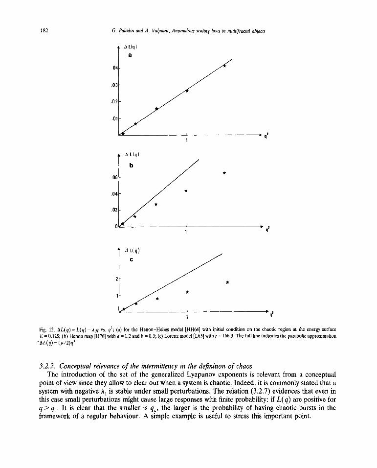
We have performed a series of numerical computationsof L(q) for the Henon—Heilesmodel[HH64], the Henonmap[H76] andthe Lorenzsystem[L63] (seefig. 12). The Henon—Heilesmodel isconsistentwith L(q) as doneby eq. (3.2.12)with /.LIA1 near1. Onthe contrary,the HenonmapandtheLorenzmodelfor r near166.07(thecritical valueof intermittencytransitionto turbulence,see[PM8O])show strong deviationsfrom the lognormalprediction.
182 G. Paladin andA. Vulpiani, Anomalousscalinglaws in inultifractal objects
A 1(q)
A L)q)
*
A 1(q)
Fig. 12. ~L(q) = L(q) — A,q vs. q2 (a) for the Henon—Heilesmodel [HH641with initial condition on the chaotic regionat the energysurface
E= 0.125; (b) Henonmap[H76]with a = 1.2andb = 0.3; (c) Lorenzmodel[L63] with r = 166.3. Thefull line indicatestheparabolicapproximation‘.~L(q)= (js/2)q2.
3.2.2. Conceptualrelevanceof the intermittencyin the definition of chaosThe introduction of the set of the generalizedLyapunov exponentsis relevantfrom a conceptual
point of view sincetheyallow to clearout whena systemis chaotic.Indeed,it is commonlystatedthatasystemwith negativeA
1 is stableunder smallperturbations.The relation(3.2.7) evidencesthat eveninthis casesmallperturbationsmight causelargeresponseswith finite probability: if L(q) arepositivefor
q> q,~It is clear that the smaller is q,~,the larger is the probability of having chaoticbursts in theframeworkof a regularbehaviour.A simple exampleis useful to stressthis importantpoint.
G. Paladin and A. Vulpiani, Anomalousscaling laws in mulcifractal objects 183
Let uscomputeL( q) in the caseof the Langevinequation:
= —dVldx+ ~ (3.2.15)
where~ is a white noise, i.e. a randomGaussianprocesswith zero averageand covariance:
(~(t) ~(t’)) = ô(t — t’) . (3.2.16)
We considertwo trajectoriesx(t) and1(t) = x(t) + s(t), both satisfying eq. (3.2.15) with the samerealizationof noise.We define:
R(x(0), rI,i) = ~ (3.2.17)
which is of coursea functional of ~. The function L( q) is then:
L(q) = lim ln J d[~]P[~] R’7(x(0),iiii) (3.2.18)
whereP[~] is the Gaussianprobabilitydistributionfunctional. Let us remarkthat the definition of theLyapunovexponentsfor stochasticequationsis a subtlemathematicalpoint; we haveherefollowed thenaive standardprocedure(seee.g. [CFU82]). Usual argumentsimply that L(q) doesnot dependonx(0). Our aim is to evaluateL(q). We first notice that:
R(x(0), Tl~) = exp[—J V”(x(t)) dt] (3.2.19)
wherethe dependenceon ~ comesthroughthe dependenceof x(t) on i~.Let us evaluate:
(R’7(r)) Jd~[x]rexp(_qfV11(x(t))dt) (3.2.20)
whered~[x]Tis the measureinducedon the trajectoriesby the stochasticdifferentialequation(3.2.15).It is well knownthat (see for example[G78]):
d~[x]T= exp(_Jdt {~(t)2 + ~1(x(t))}) d[x]T
= exp(_J~(x(t)) dt) dP[x]T (3.2.21)
wheredP[x]’~ is the usualWienermeasureon the trajectoriesandwe haveneglectedboundaryterms(i.e. termsdependingon x(0) andx(r)). The function ~l/is given by:
184 G. Paladin andA. Vulpiani, Anomalousscaling laws in multifractal objects
~l(x)= ~(dVIdx)2— ~d~VIdx~. (3.2.22)
The Feynmanpath integral representationfor quantum mechanicsat imaginary time implies that[FH63]:
JdjL[x]T —* exp(—r E0(O/l)) (3.2.23)
wherewe haveneglectedthe prefactorand E0(~ll)is the groundstateof the Hamiltonian
I = — ~ d2Idx2 + °/l(x). (3.2.24)
ConsistencyrequiresthatE0(~U)= 0, which is indeedtrivial to check. We can now write:
(R~(r)) J d[x]T exP(_/dt[~i(t)2 + ~(x) + q V”(x)])
ccexp(—rE0(q)) - (3.2.25)
whereE0(q) is the groundstateof the Hamiltonian
l~(q)= —~ d2/dx2+ t~/l(x)+ q V”(x). (3.2.26)
It is clear that
L(q) = —E0(q). (3.2.27)
Equation(3.2.27)gives a methodto computeL( q) in anapproximateway. A few exact solutionsareavailable:for exampleif V= x
2 we haveL(q) = —2q. In the generalcasewe remarkthatlimq~,.L(q)Iq = _L* is easyto computeandit is given by L* = mini V”(x). This meansthat, althoughL(q) can benegativefor smallq andthe systemis stablein theusualsense,the systemcan beunstableundera smallperturbationas soonas V”(x) is negativesomewhereas previously discussed.
We remarkthat this situationis somehowsimilar to what happensin the caseof a multifractal set inboth fully developed turbulence and chaotic attractors: the strongest singularity dominates thebehaviourof the high momentsfor the structurefunctions [BPPV84];for a similar casein differentcontextsee [B77, B82].
3.2.3. GeneralizedLyapunovexponentsof higher orderA more accuratedescriptionof the chaoticity in a dynamicalsystemcan be achievedby taking into
accountthe fluctuationsin the divergenceof volumesin phasespaceunderthe dynamics.Toward thisgoal, we can definea setof generalizedLyapunovexponentsof ordern which generalizethe relation(3.2.7) [PV86b]:
= Jim ~ ln(R~-”~(t)’7) (3.2.28)
G. Paladin and A. Vulpiani, Anomalousscaling laws in multifractal objects 185
whereL”’(q) = L(q). It is theneasyto verify that:
~ A, = . (3.2.29)dq q=O
The wholespectrumof the Lyapunovexponent{ A1, A2,... AF } hasnow found its counterpartbut itseemsratherartificial to distinguishthe contributionof eacheigendirectionê, in the fluctuationsof theexponentialdivergenceof an n-dimensionalvolume. One is of coursetemptedto define:
l,(q) = L~’~(q)_qL(~~1)(~) (3.2.30)
with F�i�2 and I1(q)=L(q)Iq.
This definition is howeverjustified only by the trivial fact that l,(O) = A,. Moreoversomepreliminaryresults[G86a]indicatethat it cannotbe correct for systemswhich are not hyperbolicwherethe stableandunstablemanifoldscan mix eachotherunderthe dynamics.The measurablequantitiesarejusttheL~ andwe can repeatfor them all the considerationsdonefor L(q).
We want to stressthatL~(q)as well as L(q) cannotbe extractedby an experimentalsignal whilethey can be easily computedfrom the numericalanalysisof a dynamicalsystemevolution using themethodsdevelopedby Benettin et al. [BGGS8O]evenif someprecautionsmustbe takenin order toavoid computeroverflows due to the fastdivergenceof R’7.
3.3. The Renyi entropies
The Kolmogorov entropy is relatedto the sumof the positive Lyapunovexponentswhich measurethe divergencerate along the expandingdirections. IndeedPesin [P77]proved that for an ergodicmeasurewith a compactsupport
K1 � A~ (3.3.1)
wherep is -thenumberof exponentsA, >0. In manyinterestingsituations,for examplethe Hamiltoniansystems,(3.3.1) becomesthe identity [ER85]:
dL~’~K1 = ~ A. = (3.3.2)
1=1 uq qO
which we shall assumevalid in the following.On the other hand, temporal intermittency correspondsto fluctuationsin the predictability time
which can be describedby a set of generalizedentropiescalled in the information theory Renyientropies[R70].
Let us give their definition in a simpleconstructiveway which can be mademore rigorouswithoutexcessivedifficulties, seee.g. [CP85].Take a recordof measuresof a signal x(t) atuniform spacingr:
x,=x(ir) withi=1,2,...M~1 (3.3.3)
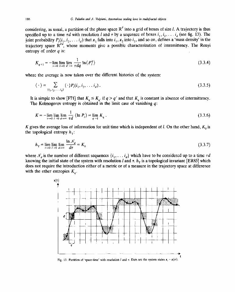
186 G. Paladin and A. Vulpiani, Anomalousscaling laws in multifractalobjects
considering,as usual,a partition of the phasespaceR’~into a grid of boxesof size1. A trajectoryis thusspecifiedup to a time Td with resolution I andT by a sequenceof boxesi1, ~ i~(seefig. 13). Thejoint probability P1(i1, i2, . . . i~)that x1 falls into i1, x~into i2, and so on, definesa ‘massdensity’ in thetrajectory space RFd, whose momentsgive a possible characterizationof intermittency. The Renyientropyof order q is:
Kq+i = —lin~~in~~im ~ ln(P~) (3.3.4)
wherethe averageis now takenover the different historiesof the system:
~ (~)P1(i~,i2,. . . ii). (3.3.5){i1,z2, - . -
It is simple to show[F71]that Kq � K~.if q> q’ andthat Kq is constantin absenceof intermittency.The Kolmogorov entropy is obtainedin the limit caseof vanishingq:
K= —limlim lim —~— (lnP1) lim K . (3.3.6)~-~O l—.0 d-~oord q-1 q
K gives the averageloss of informationfor unit timewhich is independentof 1. On theotherhand,K0 isthe topologicalentropyhT:
lnXdhT=hmllmllm =K0 (3.3.7)TO 1—~Od—~= dr
whereXd is the numberof differentsequences{i1,. . . id} which haveto beconsideredup to a time rdknowingthe initial stateof the systemwith resolution1 and ‘r. hT is atopologicalinvariant [ER85]whichdoesnot requiretheintroductioneither of a metricor of a measurein thetrajectoryspaceatdifferencewith the otherentropiesKq~
x (t)
— ~ — ~.:.
~ ---~-~~
-
Fig. 13. Partitionof ‘space-time’with resolution I and r. Dots arethe systemstatesx~= x(iT).
G. Paladin andA. Vulpiani, Anomalousscaling laws in multifractal objects 187
It is evident that the topologicalentropy is the analogueof the fractal dimensionas well as theKolmogoroventropyof the information dimension.The probability P1(i1,. . . i,~)is deducedfrom the(chaotic)temporalevolutionof the systemand,in this sense,the entropiesreferto the naturalmeasure.A more refineddefinition requiresan extremumover the possiblepartitionsof space-timebut it goesfurther than the purposesof this paper[W86, CP85].
Grassbergerand Procaccia[GP83b]havefirstly proposeda methodfor the computationof ~ (alower boundof K) which is quite analogousto that for the computationof d2. This numericalalgorithmhasbeenextendedto the calculationof K [CP85]as well as of the whole setof the Kq ‘s [PV86b].
It is worth noting that the Renyi entropiescan be extractedby an experimentalsignal while thegeneralizedLyapunovexponentscannot.Indeed,let us estimatethe average(3.3.4) by a recordof Mmeasuresat uniform spacing‘r. The joint probability P1(i1,. . . id) is thengiven for M largeenoughby:
n~(l)= M~1 ~ o(i — x~,,— ~ (3.3.8)( )j+i ni
In the limit d = 1, n~(l)becomesthe densityn.(l) of pointsin aball of centrex, andradiusI definedineq. (1.1.7).
Increasingthe time thisdensitydecreasessincemanypointswhich areinitially in the ball of centrex,do not remainin the ball around‘i+d (the d-iteratedpoint of x,). The Kolmogoroventropymeasuresthe inverseof the averagecharacteristictime of thisexponentialdecay.We can howeverdefine for eachmomentthe quantity:
C~(I,q) -~- ~ (n~(l))’7 (P7). (3.3.9)
The correspondingentropyKq+ 1 is thusgiven by the d-asymptoticvalueof the ratio:
1 / C~’l \ \limlim lim —ln( d ~ q, (3.3.10)T-.0 i-.0 d—. ‘rq \ C~+1)(i q) /
3.4. Relation betweenthe generalizedLyapunovexponentsand the Renyientropies
We can find a simple relationbetweenentropiesandgeneralizedexponentsunderthehypothesisthatthe Pesinidentity K = E ~= A. holds.
As a starting point it is convenient to define the concept of ‘mass’ M in the trajectory space.Following Grassberger[G86b], let us focus on a given trajectoryx(t) and the trajectorieswhich staywithin a distance�l from x(t) for all the time in the interval [t*, ~ + At]. One defines a domain B:
B {y(t): y(t) — x(t)~� 1, VtE [t*, t~’+ At]) . (3.4.1)
Let us denoteby M1(x(t*), At) the measureof B. Then, this massdecayswith At since thereareexpandingdirections(at least ‘in average’)correspondingto thej~positiveLyapunovexponents.Let usassumethatthe numberof contractingdirectionsdoesnot change,i.e. definingp � + 1 as thenumberof non-negativeLyapunovexponents:
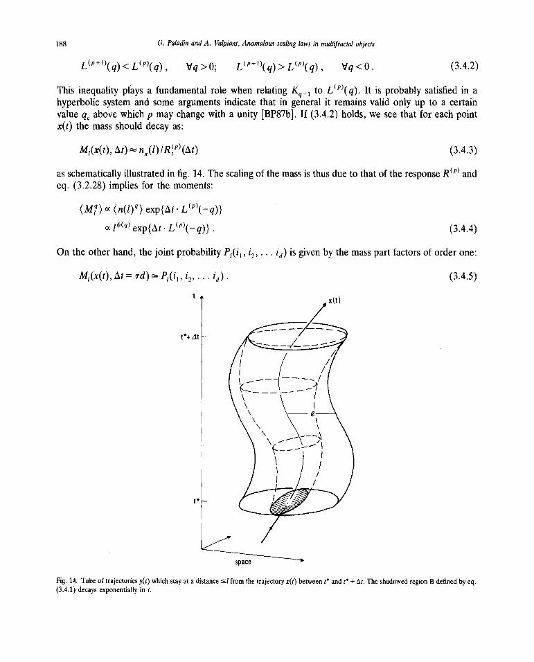
188 G. Paladin andA. Vulpiani, Anomalousscaling laws in multifracial objects
L~’1~(q)< L~”~(q), Vq >0; L~’~1~(q)>L~(q), Vq <0. (3.4.2)
This inequality plays a fundamentalrole when relating K~~1to L~”~(q).It is probably satisfiedin a
hyperbolicsystemand some argumentsindicatethat in generalit remainsvalid only up to a certainvalueq,~abovewhichp maychangewith a unity [BP87b].If (3.4.2) holds, we see that for eachpointx(t) the massshould decayas:
M1(x(t),At) — n~(l)IR,~’~(At) (3.4.3)
as schematicallyillustratedin fig. 14. The scalingof the massis thusdueto that of the response~ andeq. (3.2.28) implies for the moments:
(M7) cc (n(l)~)exp{At-~L~’~(—q)}
cc ~ exp{At. L~(—q)}. (3.4.4)
On the otherhand,thejoint probability P~(i1,i2,. . . id) is given by the masspart factorsof orderone:
M1(x(t),At = rd) P1(i1, i2, . . . ~d) . (3.4.5)~ 7
\\ ~-::;\
Fig. 14. Tubeof trajectoriesy(t) which stayat adistance~l from thetrajectoryx(t) betweent~andt~+ ~t. TheshadowedregionB definedby eq.(3.4.1) decaysexponentiallyin t.
G. Paladin and A. Vulpiani, Anomalousscaling laws in multifractal objects 189
We can thereforeestimatethe averagein (3.4.4) by a weightedsum over the possiblesequencesofboxes{i1, ~ . id}:
(M7) = ~ P~(i1,i2,.. . i~)’7~1ccexp(_rdqKq~
1). (3.4.6){‘1.~2’- - - ‘d}
It follows, by comparing(3.4.6) and (3.4.4), the relation [PV86b]
L~(—)
Kq±1= —q (3.4.7)Equation(3.4.7)becomesthe Pesinidentity in the limit q—*0 while hT, the topologicalentropyK0, isequalto L P)( 1), the exponentwhich rules the exponentialdivergence,in average,of a p-dimensionalvolume underthe chaoticdynamics.
3.5. Multifractality in the trajectory space
We can regardthe set of trajectories(box sequences)of an intermittent systemas a multifractalobjectwith regardto the mass definedin eq. (3.4.1).
Let us namelycall historyX~the finite sequenceof measurementsof the signal x(t):
(xk, Xk+1, . X~_~) (3.5.1)
wherex,, = x(kT).x~representsapoint in the history spaceRF ® R’~ ® RF (d times). We also introducea metric
by defining the distancebetweentwo trajectoriesas:
— y(d)) = sup Xk+J — Y,,+i~. (3.5.2)
Oajad—1
Aroundeach historyX~thereis a tubeT of trajectoriesY~suchthat:
~ d) = {Yk: ~(y~J) — X~)~ 1) . (3.5.3)
A naturalmeasurein the spaceof historiesis introducedif the initial statex, is distributedaccordingtothe invariant naturalmeasureon the attractor.We can thusdefinethe probability P1(X~)that a givenhistory falls within the tubeT1 aroundX~.Suchaprobability can be estimated[GP83a,GP83b]if weknow a greatnumberX of historiesX(1N) (or a very long record of consecutivestatesof the system,which is then brokenup into historiesof lengthN). One has:
P1(X~)—~~ 0(1—~(X~ —x~)). (3.5.4)
This probability decreasesexponentiallywith a characteristictime y 1 which dependson the particularinitial conditionx,,.
190 G. Paladin and A. Vulpiani, Anomalousscaling laws in multifractalobjects
P1(X~)cc eT~~ for large times. (3.5.5)
The temporal intermittencyis thuscharacterizedby the fluctuationsof theselocal expansionparame-ters, LEP, y. It is not difficult to apply the multifractal approach[EP86, PPV86, SSS86] to thedistributionof ‘y in the sameway as the distributionof a for the phasespacehasbeencharacterized.
It is convenientat this point to divide the spaceof historiesinto boxesof linear size I. The ‘history’boxesare thenthe cartesianproduct (for 1 <j < d) of the ‘phasespace’ boxes.The time evolutionofthe systemis thusgiven by a particular history box I = (i1,. . . id) as we haveseenin the section3.3.The joint probability P1(i1,. . . id) is the probability P~(I)that a historyX~belongsto the box I.
We now considerthe set f2(y) of historieswhose LEP belongs to the interval [y, y + dy]. Thenumber.N’7 of boxesnecessaryto coverthis set will increasewith d accordingto the law:
.N’~(d)ccexp(rd h(y)) (3.5.6)
whereh(y) is the topologicalentropy of the set fl(y), with the warning that if h(y) � 0, thenthetopologicalentropy is zero. We haveby definition h(y) � hT.
Let usnow showthat h( ‘y) and Kq arerelatedto eachotherby aLegendretransformanalogousto(1.2.5).
Indeed,the partition of the (multifractal) set of the historiesinto the setsQ( y) allows to computethe averages(3.3.4)as weightedsumsoverthe boxesI, by groupingtogetherall the boxeswhichbelongto the same(1(y):
(P~(I)’7~)=~ P1(Iyl{I}
cc Jdp(y)exp(—dT(qy — h(y))) (3.5.7)
wheredp(’y) is a smoothmeasure.A saddlepoint estimationof the integralyields in the limit of large rd:
K~(q— 1) = mm (q’y — h(y)). (3.5.8)
The term exp(—dr) is herethe scaling parameterin the history spacelike 1 in the phasespace.Let usemphasizethat the probability that a trajectory (i.e. a box I) belongsto a set fl( y) scalesas:
~P(XE.Q(y))ccexp(—S(y)rd) (3.5.9)
with S(y)�0.Argumentsquite similar to thosewhich leadto eq. (1.2.11)showthat:
(P7) = f ~(XEfl(y)) ~rdyq dy (3.5.10)
andso:
G. Paladin and A. Vulpiani, Anomalousscaling laws in multifractal objects 191
K~~1q= mm (qy + S(y)). (3.5.11)
It follows by comparing(3.5.8) and (3.5.11)that:
S(y)=—h(y)+y. (3.5.12)
The equalityS = 0 holdsonly for y = K1 implying that in the asymptoticlimit t—* cc one hasvanishingprobabilityof finding a trajectorywith LEP differentfrom the Kolmogorov entropy.Eachq peaksup aparticularvalueof the LEP by minimizing (3.5.8) or (3.5.11):
q = dh/dy~(~) and q = —dSIdyI~(~). (3.5.13)
In the limit q --* ±ccthe Legendretransformbecomestrivial andone finds the extremabetweenwhich y is bounded:
Ymin~K= and 7max=K~. (3.5.14)
At q = 0, j = K* (and ~ = K1) whereash attainsits maximum:
h(y= K*) = K0. (3.5.15)
S hasits minimumat K1: S(K1)= 0. It is easyto showthat h (and— S) areconvexfunctionsdefinedonthe interval [K,~,K_,,j; S hasa quadraticminimum implying for y K1 the parabolicshape:
S(y) = (y — K1)212b. (3.5.16)
Let usnotethath(y) is also approximatedby a parabolaaroundK1 andnot aroundits vertexK*. For
smallenoughq we thenhave:
- Kq±i=Ki~~bq (3.5.17)
whereb is the second-ordercumulant:
b = lim lim lim —k— [(ln2 P
1(I)) — (ln P1(I))2] . (3.5.18)
r-.0 1—~0d—.oc rd
For a lognormal distribution of the ‘mass’ in the trajectory spacethe relations(3.5.16) and (3.5.17)remainvalid for all the q values.
The relationbetween— S(y) andKq+ 1 is reminiscentof that linking theentropyto thefree energyinthermodynamics/3 F( /3) = U( /3) — .9°(/3). The role of the inverseof the temperature/3 is playedby themomentindex q, F(/3) by ~ U by j and .9°(/3)by —S(~(q)).
Let us limit ourselvesto considerthe branchof positive temperatures(i.e. q >0). As q—~ cc (i.e.vanishingtemperature)the systemis found in the stateof minimal energyYmin and minimal entropy~S(Ymin).
A typical phasediagramof Kq vs. q is shownin fig. 15.
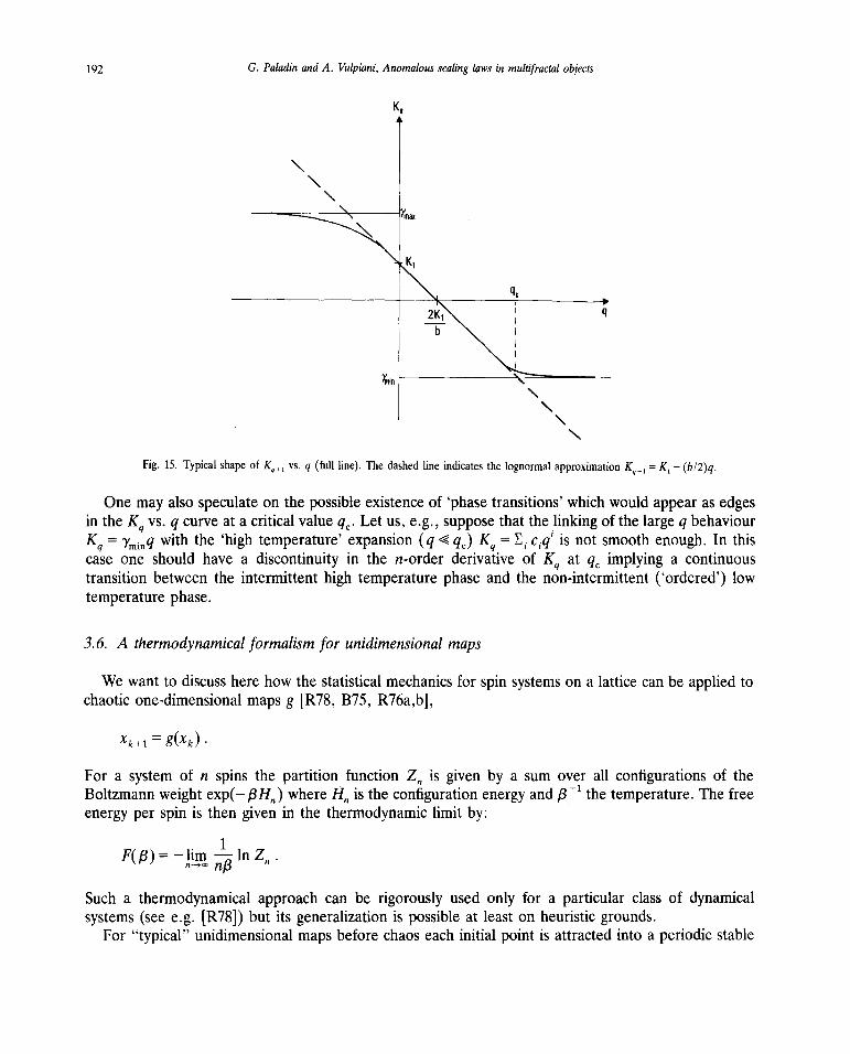
192 G. Paladin andA. Vulpiani, Anomalousscaling laws in multifractal objects
~‘ifl
NN
N
Fig. 15. Typical shapeof Kq*j vs. q (full line). The dashedline indicatesthe lognormalapproximationK,~,= K~— (b/2)q.
Onemayalsospeculateon the possibleexistenceof ‘phasetransitions’whichwould appearas edgesin the Kq vs. q curveat a critical valueq,~.Let us,e.g.,supposethat the linking of the largeq behaviourKq = y~,qwith the ‘high temperature’expansion(q ~ q,~)Kq = ~, c,q’ is not smoothenough.In thiscaseone should have a discontinuity in the n-order derivative of Kq at q~implying a continuoustransitionbetweenthe intermittenthigh temperaturephaseand the non-intermittent(‘ordered’) lowtemperaturephase.
3.6. A thermodynamicalformalismfor unidimensionalmaps
We want to discussherehow the statisticalmechanicsfor spin systemson a lattice can be appliedtochaoticone-dimensionalmapsg [R78, B75, R76a,b],
Xk+l = g(x~)
For a systemof n spins the partition function Z,, is given by a sum over all configurationsof theBoltzmannweightexp(— /3H,,) whereH,, is the configurationenergyand~31 the temperature.The freeenergyper spin is thengiven in the thermodynamiclimit by:
F(/3)=—1im--~lnZ,,.
Such a thermodynamicalapproachcan be rigorously usedonly for a particular class of dynamicalsystems(seee.g. [R78]) but its generalizationis possibleat leaston heuristicgrounds.
For “typical” unidimensionalmapsbefore chaoseachinitial point is attractedinto a periodic stable
G. Paladin andA. Vulpiani,Anomalousscaling laws in multifractal objects 193
orbit suchthat Xk = g~(x~)whereg~is the nth iterateof g. The evolutionbecomeschaoticwhereasall the orbits becomeunstable.Nevertheless,the statisticalpropertiescan still be characterizedby theseunslableperiodic orbits [B79].
A global degreeof instability is measuredby the Lyapunovexponents[MR82]:
A=limfd~L,,(x)lnIg’(x)I (3.6.1)
whereg’ = dgldx anddp~is an invariant measurewhich convergeswith n to the invariant ergodicmeasured~t(x).
Kai and Tomita [KT82] suggestedthe following form for p~,:
X(n)
~ a.6(x—z,) (3.6.2)
where z~are the X(n) unstablefixed points of period n (i.e. z~= g”(z1)), the set of which will bedenotedby J(’~)•Its cardinalityX(n) is proportionalto exp(hTn)by definition.
The weighta, for measureswhich are absolutelycontinuouswith respectto the Lebesguemeasure[L81] is:
a = c,,I~g°’~(z~)’~with ~ a, = 1. (3.6.3)
We can thus define a partition function following Takahashiand Oono [TO84]:
Z,,(g, /3) = ~ exp{—/3~ (3.6.4)
The fluctuation of the degreeof chaoscan be characterizedvarying /3 by the generalizedLyapunovexponents.Let us in fact call R~(z) = (g~(z))’J the responseafter n iterations of the map to aperturbationin z, unstableperiodic solution of ordern.
The partition function (3.6.4) becomes:
Z,,(g, /3) = ~ exp{—/3 ln R,,(z~)} (3.6.5)z1EJ
1”t
which can be estimatedby a time average in the chaotic phase. Moreover, let us recall theBowen—Ruellerelation [B75]:
F(g, /3=DH)=0 (3.6.6)
whereDH is the Hausdorffdimension.The definition of Hausdorifdimensionrequiresa minimumoverthe possiblepartitions into boxes of size si for l—* 0. We haveescapedthesetroublesconsideringuniform partitionsinto boxesof size I. If theseproceduresareequivalent(which is often true), thentheHausdorffdimensionis the fractal dimension.
For measureswhose support is fractal, the ansatz (3.6.3) suggests to assume the weighta, cc g~(z
1)’ ~ which correspondsto a “uniform” measurefor which 4(q) = ~ q [BPPV85].
194 G. Paladin andA. Vulpiani,Anomalousscaling laws in multifracial objects
The partition function (3.6.5) can be - estimated by an ensemble average (.) =
~z1EJ(”~ ~ for large n:
Z~(g,/3) = (R~~F)= R~P+DF (3.6.7)
where (~) is a time average.ThegeneralizedLyapunovexponentscomputedwith respectto the uniform measurethereforeallow
one to determinethe free energyF( /3) by the relation:
P(/3) = —/3F(g,/3) = L(q = (DF — /3)), (3.6.8)
wherewe haveintroducedthe so-calledtopologicalpressureP( /3).The Bowen—Ruelleformula (3.6.6)now simply follows from the trivial identity L( q = 0) = 0.It is useful to note that the temperatureparametrizesa whole classof probability measures(called
Gibbs equilibrium measures)on the invariantsetJ given by the closureof lim,,...~00J~”~:
d~(x)= lim ~ dx 6(z, — x) ~ , (3.6.9)ziEJ (~)
where /3 = DF picks up the uniform measure.A moment of reflection shows that the characteristicLyapunovexponentA~
ti~computedby an averageover the measure~ is:
A(~)—~(ln~g’(x)~ usJdi~(x)ln~g’(x)~. (3.6.10)
It correspondsto an internalenergyU( /3) definedas:
U — F 1 dlnZ~(/3) — dpH n—~fl d/3 d/3~
Let us notethat the Pesinequality is not satisfiedif DF < 1 sinceone has [LM85,G86b]:
K1(i) = A(~t)~D1(~), (3.6.11)
and D1(~) � DF for any measure~. Nevertheless,for the uniform measurewhereD1 = DF we canextendrelation (3.4.7) [BPTV87],which becomes
Kq+i = —L(—DF~q)Iq. (3.6.12)
Let us also discussthe limit of infinite temperature/3 —*0, which picks up the maximumentropymeasure(3.6.5)suchthat K1 = hT = max~K1(p~)andKq = hT for all q. Relation(3.6.5)now givesthenumberX(n) of unstablefixed pointsof period n. In the limit n—* cc we find that:
hT=lim lnX(n) =-lim/3F(/3)=P(0). (3.6.13)
G. Paladin andA - Vulpiani,Anomalousscalinglaws in multifractalobjects 195
We finally notethat (3.6.6)can beextendedto a genericalq value in thecaseof the uniform measure[BPTV87] and of the maximum entropy measure[LPC87,T86,F87] to P(D~q)= (1 — q)Kq andP(—çb(q)) = (q + 1)hT, respectively.
3.7. Partial dimensions and entropies
The introduction of dimensions and entropies related to the different eigendirectionsof thelinearized flow allows to find some relations linking Renyi dimensions to Renyi entropiesand togeneralizedLyapunovexponents,evenif its applicability seemsratherquestionableas notedin section3.2.
Let usassumethat asmallbox centredarounda point x1 of the trajectoryis stretchedalongthe ktheigendirectionby a factor
mk(xl, t) cc exp{yk(x,)~t} for large t (3.7.1)
whereonecan easily recognizefrom the definition (3.2.30)that
(m~)ccexp{i~(q).t}, (yk)=Ak forlarget. (3.7.2)
In the same spirit, Grassberger[G86] proposedto assign a ‘partial dimension’ Dq(k) to eacheigendirection.The Renyi dimensionsaregiven by the sum of all the partial dimensions:
dq=~Dq(k). (3.7.3)
The attractoris thus decomposedin the direct product of continua (directionswith D1 = 1), discretepoints (D1 0) and Cantorlike sets (D1 <0).
Following ref. [BP87a]with slightmodifications,let us definea (generalized)volume contractionrateof orderq arounda point x,:
~(q, t) = ~ (3.7.4)
The averagevolume conservationthenimplies the relation:
urn (V(q, t)~) = 1. (3.7.5)
This is a constrainton the choice of the proper dimensionlist of the Dq +i’s. In the limit q—*0,condition (3.7.5) becomes:
D1(k) Ak = 0 (3.7.6)
and it is possibleto show [G86a]that the Kolmogorov entropyis given by:
196 G. Paladin and A. Vulpiani, Anomalousscaling laws in multifracial objects
(+)
K1=~ Dl(k)Ak (3.7.7)
wherethe sum ~ runsover the directionswith positiveAk. The Pesinrelation(3.3.2) is recoveredifall the expandingdirectionshavedimensionsD1 = 1 as it is the case of axiom A systems [ER85].
Furthermore,for q � 0 the partial dimensionmust satisfy the constraint
0:SDqSl. (3.7.8)
The simplestchoicecompatiblewith (3.7.5) and(3.7.8) is given by the assumptionthat the attractorisCantor-like only alongthe (j + 1 )th direction, where j is the largest integer for which E = 1 Ak � 0. Wehave Dq(k) = 1 for k ~ j, Dq(k)= 0 for k>1 + 2 and Dq( I + 1) ~ 0 as well as �1. This choicemaximizesthe estimationof the information entropyand gives the Kaplan—Yorke formula [KY78]:
d1 =j + ~ Ak/~AI+IL (3.7.9)
Equation(3.7.9) is in generalan upperboundbut it hasbeenprovedto be exactfor two-dimensionaldiffeomorphisms [Y82]. Analogous upper bounds can be obtained for dq+1 with q >0. However,in thecase of maps with more than two degrees of freedom, one needs to assign several trial values of Dq+ 1 inorderto determinethe right onesby interpolation.It was proposed[BP87a]to decreasethe dimensionsDq(k) starting from the largest possible list (Dq = 1 for k= 1, 2,. . . F) until the requirement(3.7.5) issatisfied. In this procedure one always imposes that only one direction, say Jq’ is Cantor-likewhereJq isthe largestinteger for which:
1 j ~—1/qlim — ln(,fl mk(t),) �0. (3.7.10)~ k=1
In this way, we obtain Dq(Jq + 1) from (3.7.5) and thus an upperbound for dq. Only in the case oftwo-dimensionalmapswith constantJacobian,the equalitydq = Iq + Dq ( Iq + 1) canbe explicitly solved[BP87a].
Nevertheless,it is possible to perform a perturbative expansionof eq. (3.7.10) defining thegeneratingfunction g:
~flmkk)ccexp{g(z1, z2,. . . zF)t}, (3.7.11)
for large t.
The averageconservationof the volume (3.7.5) implies that [G86b]:
g({zk=Dq+l(k)~q))=0 (3.7.12)
with:
g(z1,z2,. . . z~)= ~ z~A1+ ~ z1QjkZk + (3.7.13)
noting A1 = (y1) and QIk = ((~— A~)(~— Ak)).
G. Paladin and A. Vulpiani, Anomalousscalinglaws in mulnfractalobjects 197
The generalizationof the Kaplan—Yorkeformula (3.7.9) is thengiven by inserting eq. (3.7.13)intoeq. (3.7.12) so that:
~ Dq+i(k) Ak = ~ ~Dq+i (i) QikDq+l(I~) ~ (3.7.14)
It is also possibleto find the analogueof relation (3.7.7):
(+) (+)
Kq+i = ~ A,, — ~ Dq+i(k) Qk,1Dq+i(j) (3.7.15)
which in the limit of axiom A systemreducesitself to a Pesin-like equality:
(+) (+) L~’~Kq+1=~ Ak—~~ Q~,J+o(q
2)= q~ (3.7.16)
We must finally discussthe connectionswith the thermodynamicformalism.As the conservationlaws(3.7.5) involve both Renyi dimensionsand Renyi entropies,Badii and Politi [BP87b]arguethat thefunctionH(a) is relatedto theanalogousS(y), respectivelydefinedin eqs. (1.2.9)and(3.5.9). Indeed,underthe hypothesisthat to eachsingularity~ correspondsagivenlocal expandingparameter~,we canidentify the factore aroundapoint x, of the trajectorywith the scalingof the measurel~.It followsthat:
exp(—r y(x1)) cc I°~’~ (3.7.17)
andthe probability of finding a singularitya in the range [~, i + da]
~P(~)cc l’~~cc exp(—r~H(ii)I~)
should scaleas the probability P(j~)ccexp{—S(~)T} of finding a LEP E [~, j + d’y].This implies that
H(a)Ia = S(y)/y. (3.7.18)
The appearanceof discontinuitiesin the Renyi functionscan be analysedin termsof partialdimensions.If the index ‘q’ at which Dq+i(Jq) � 0 and ~1, is not fixed but jumps by one unit at q~,we should
expect an edge in the Renyi dimensions.In this case, the partial dimensionassociatedwith theCantor-like direction for q > q, decreaseswith increasingq andvanishesfor q � q,~.The precedingdimensionDq+i(Jq — 1) which is equalto 1 for q � q~begins to decrease with q, at the sametime.
This involvesa kind of first-orderphasetransitionin the function dq+ 1 (regardedas a free energyatthe inversetemperature/3 = q) correspondingto vanishingof the contributionof the multiplier rn tothe generalizedvolume (3.7.4)at q,~.We can correctly speakof transitionif the ‘Kaplan—Yorke’ choicefor the list of Dq is not only an upperboundbut coincideswith the real Dq’S. Otherwisethe transitioncan be relatedto the changein the rule used to definethe partial dimensions.
We have describeda mechanismwhich can explain the appearanceof ‘phase transition’ just forsystemswhereeacheigendirectionhas its ownindividuality. On the otherhand,in genericsystems,like
198 G. Paladin andA. Vulpiani, Anomalousscaling laws in multifractal objects
the Henon map, an expandingdirection can coincide with a contractingone when it is computedatdifferentpoints. For q largerthanq~a transitioncan occurbecauseof an exchangeof two multipliers.
This secondmechanismis not yet fully understoodand we refer the readerto [BGP87] for moredetails.
4. Replicasof disorderedsystemsas multifractal objects
4.1. Introduction
The techniquesdevelopedfor the characterizationof the temporalintermittencyarequite usefulforthe study of disordered systems. Indeed, in some systems, the sample to sample fluctuations of thephysical observables can be described in terms of the generalized Lyapunov exponents related to theproductof appropriatetransfermatriceswhoseelementsarerandomvariables.We havehereto notethat the randommatrix product is a ratherinterestingproblemalso in dynamicalsystemswhereit isoften usedas amodelof the chaoticbehaviourof quasi-integrableHamiltoniansystems[B84, PV86a].
In this sectionwe want to showhow the different realizationsof the systemwith respectto disordercorrespondto trajectoriesgeneratedby iterating the transfermatrices.
It is thus possible to define a multifractal object in the ‘replica ensemble’: in this sensethefluctuationsinducedby the disorderare an intermittencyphenomenon.
We must however stressthe peculiarity of this sort of intermittency. In a time evolution thecharacterization of the degree of chaos variations has a great practical relevance. One is interested inthe knowledgeof the (chaotic)signal as function of time andnot only in the ‘global’ behaviour.On theotherhand, the fluctuationsaroundthe averagevaluein adisorderedsystemareratherlessimportantsince they decay exponentially with volume in the thermodynamic limit which is always reached in areal sample.
The multifractal formalism becomes in this case just a fluctuation theory which is quite analogous tothat introducedby Einstein in the canonicalensemble.
Let us in fact consider a large number of different samples of a usual equilibrium system with Nparticles. A sample can of course be regarded just as a ‘small’ part of a larger system. Each sample isthen characterized by its energy per particle, say x, andwe can group all the realizations with energyper particle between x andx + dx in the same set 11(x). The numberH,~of realizations belonging to11(x) is assumed to increase exponentially with N like:
H~—.-exp(s(x)N), (4.1.1)
wheres(x) is the microcanonicalentropyper particle correspondingto the energyx.
We can now computethe partition function of the Gibbs distributionintegratingover x:
ZN(/3) = f H~e~ dx — J ~ dx. (4.1.2)
In the limit N—*cc only one setgives a relevantcontributionto ZN. By means of the steepest descentmethod one in fact gets:
G. Paladin and A. Vulpiani, Anomalousscaling laws in multifractal objects 199
ZN(/3)~exp(-/3f(/3)N) (4.1.3)
with
/3f(/3)=min[/3x—s(x)]=13u—s(u)
wherethe minimal conditionin the Legendretransformation(4.1.3) implies:
=/3(u). (4.1.4)dx
The probability of finding a samplewith x ~ u vanishesfor largeN like:
PN(x) = Z~1~ FI~— exp(—/3N[~(x)—f(/3)]) (4.1.5)
where ~/i~ = /3x — s(x)� f andf is the free energyper particle of the system.We havederivedthesewell-known resultsin orderto point out that the hierarchyof sets11(x) can be investigatedby varyingthe temperature.The sameapproachcan be usedfor characterizingthe finite volume fluctuationsindisorderedsystemsby meansof the replica formalism.
We shall explicitly considertwo models:the Schroedingerequationwith a randompotentialandtheIsing modelwith randomcouplings,analysingrespectivelythe localization lengthandthe free energy.A short discussionwill finally dealwith the possibilitythat thereexist ‘phase’ transitionsin the diagramL(q) versusq.
4.2. The one-dimensional Anderson model
A first simple model of the conductivity in a disorderedmedium is given by the Schroedingerequationwith a randomlydistributedpotentialV,. We shall considera discreteversionof the Andersonmodel [A58] definedon a one-dimensionallattice. One can write the finite differenceequation:
+ + wV,i/i, = E’/i, (4.2.1)
where i labels the site of the lattice, ~/‘~is the amplitudeof the eigenfunctionat the site i, V1 a randompotentialand E + 2 the energy.
In the following each V1 is uniformly distributedon the range[—112,1/2] andis uncorrelatedfromone site to another:
(v,) = 0, (V1V1)= A2~11 (4.2.2)
withA2=1/12.
It is well known that wheneverw ~ 0 the eigenfunctionis exponentiallylocalized [DLS85]. Thismeans that if we have assumedperiodic boundary conditions (i.e. IIJN = ‘l’-N) an eigenfunction{ ~ I — N � n < N) exponentiallydecreases(with probabilityone) at largedistancesaroundits maximum(say for n = 0):
200 G. Paladin and A. Vulpiani, Anomalousscaling laws in multifractal objects
I~l’nI ~ I~hIexp(—const. nI). (4.2.3)
The localizationlengthis thenusually definedas
~‘= lim --~-(lnI~,,l) (4.2.4)InI-.= fl
wherethe averageis takenover disorder.On the otherhand Mielke and Wegner[MW85] haverecently considered:
= lirn- ln (k~~I). (4.2.5)
Let us generalize(4.2.5) introducing~q[PV87b]:
lim -~—ln(l~,,I~). (4.2.6)ini-.= n~q
A direct numericalcomputationof is a hard task since it is ratherdifficult to calculatethe exacteigenvalueand eigenvectorof (4.2.1) for largechains.
Let us show that the problem can be reducedto the calculation of the generalizedLyapunovexponentsassociatedwith aproductof randommatrices.Equation(4.2.1)can in factbe written in therecursiveform:
Z(i + 1) = A~(i)Z(i) (4.2.7)
where
A~(i)=(E_wVi ~),Z(i)= (~1). (4.2.8)
One hasa productFI~A~(i)of randomsymplecticmatriceswhich relatesZ(N) to Z(0).It is useful to introducethe ‘response’after n sites whosevalue dependson the starting site m:
Rm(n)= Z(m + n)I / Z(m)I. (4.2.9)
ThegeneralizedLyapunovexponentsL(q) are thengiven by the asymptoticbehaviourof themoments:
(R(N)~)= ~ R~(N)~—exp{L(q)N) for largeN. (4.2.10)
It is easyto recognizethat ~ is the maximalLyapunovexponentA1:
= A1 = (ln R(N)) = ~ q’0 (4.2.11)
G. Paladin and A. Vulpiani, Anomalousscaling laws in mullifractal objects 201
We haveseenthat a linear behaviourL( q) = A1q indicatesthat thereare no fluctuationsof R (i.e. nointermittency).By comparing(4.2.10)with (4.2.6) one has,sinceRm(n)~~~I~I’mI”$’l’m+nI
= L(q)/q. (4.2.12)
Let usemphasizethat the sequence{Z(m + i) with 0< i <N) generatedby iteratingthetransfermatrixis not an eigenfunction{ ~/i~)on the lattice becauseit doesnot take into accountboundaryconditions.Nevertheless,if eigenstatesat the chosenenergyexist, thenthe LyapunovexponentA1 coincideswiththe inverseof the (average)localization length~. On the otherhand,the localizationlengthfluctuatesaround~ with varying realizationsof disorder.Let us thereforedefine a local expansionparameterLEP y by the relation:
Rm(N)— exp{’y(m) N) for N large. (4.2.13)
y is a random variable which dependson the starting site m and with averagevalue A1, whoseprobability distributionP(y) coincideswith the distributionof the localizationlengthsamongdifferentrealizationsof disorder.
At this point wecan apply all the multifractal machineryof the previoussectionby grouping in thesamesubsetall the trajectories{Z(m + i), 0< i < N) which haveaLEP in the range[y, y + dy].
It is quite reasonableto assumethatafter N sites the probability P(y) of havingaresponsewith agiven LEP hasthe following form:
dPN(y) = dp(y) exp{—S(y)N}. (4.2.14)
The ansatz (4.2.14)is necessaryin order to obtain anexponentialbehaviourfor the moments(R “(N))and is similar to the hypothesismadefor the singularity structure in turbulenceand in other strangesets.We can now calculatethe averageover the disorderby the averageover the y-distribution:
(R”(N)) cc Jdp(y) exp{[yq — S(y)]N} cc exp{L(q)N). (4.2.15)
A saddlepoint estimationof (4.2.15)gives:
L(q) = max[yq — S(y)]= qç1. (4.2.16)
Fromeq. (4.2.13)all the ~~‘smustbe positiveimplying y >0: whenall the potentialsV1 areequalonerecoversthe pure systemand this correspondsto the minimal value of the LEP Ymin• More generallyonecan see from eq. (4.2.16)that:
urn ~ = Ymax’ ~!~rfi~ = 7. = 0 (4.2.17a)-
0 ~ S(y) :S max[S(ymax), S(Vmjn)]. (4.2.17b)
Let us recall that S(y = A1) = 0 while S(y ~ A1) is positive in the S-definition range [0, Ymax]. The
fluctuationsaroundA1 thereforedecaywith N as exp(— y )N). The existenceof this thermodynamical
202 G. Paladin and A. Vulpiani, Anomalousscaling lawsin multifractal objects
limit correspondsto the Oseledectheorem[068] on the existenceof the LyapunovexponentA1. Theabsenceof fluctuationsis analogousto anon-intermittentchaoticbehavior.If the responseis obtainedas the productof independentrandomvariables,the lognormaldistribution is a good approximationandS(y) is a parabolatruncatedat Ymjfl = 0 andat 7max~The correspondingform L(q) = A1q + (~!2)q
2is thenvalid only for not too large q values (seeappendixB).
4.3. Anomalousscalinglaws at the band edge
For a puresystem(w = 0) the energiesof the Hamiltonian (4.2.1) areconcentratedwithin a band-2sEs2.
In the sequel,we shall limit ourselvesto the case (V1) = 0 since it is alwayspossibleto includethe
averagevalue of the potentialin the definitionof E. Let usconcentrateon the bandedgeE = 2 of thepure systemwhere the generalizedLyapunov exponentshave a particularly interesting scaling be-haviour with respect to the disorder amplitude w [PV87b]. The weak disorder expansionof theLyapunovexponentis non-analyticandone finds [DG84]:
A1 = C1w213, C
1 =0.2893A213. (4.3.1)
On the otherhandit is quite simple to extenda perturbativecalculationof Parisi andVulpiani [PVu86]
for computingL(2) in our case:L(2) = 2C
2w213 (4.3.2)
with C2 = A
2/s2U3I2~0.6299A2/l.Onecanthereforeestimatethe variance/L by assumingthat for low disorderL(q) = A
1q + (~/ 2) q2
hasa parabolicshapeup to q >2:
= L(2) /2 — A1 0.3406A
213w213. (4.3.3)
Figure 16 shows the plot of L(q) /(C2w
213q) for different valuesof w in the caseof V1- uniformlydistributedin the range[—1/2,1/2]. We observea linearbehaviourL(q)/q = A
1 + (pJ2)qfor q< tj(w)which breaksdown for larger q’s andthensaturatesto the plateauL(q)Iq = Ymax for q> ~(w).
The maximal LEP can be estimatedby a rather naive (but stringent) argument.The maximaleigenvalueof a randommatrix A~(i)is 1(V,) = 1 + + 0(w). It follows that the maximalLEP isobtainedfor a disorder realizationsuch that V~are typically of the sameorderof max{V~}=
Ymax cc wi’2 (4.3.4)
for small w.This result is in good agreementwith the numericalextrapolationof L( q) Iq in the limit of largeq
(seefig. 17).The valueof ci(w) can easilybe obtainedby matchingthe asymptoticbehaviourL(q) cc w~2with the
lognormalonefor smallq, i.e. L(q)/q = A1 + (~t/2)q.Onethusobtainst~(w)ccw~
6.Thesetwo kindsof behaviourfor L(q) (i.e. L(q) cc w213 for smallq andL(q) cc w112 for largeq) implies a crossoverforthe scalinglaw of when q is very large (seeeq. (4.2.12)).
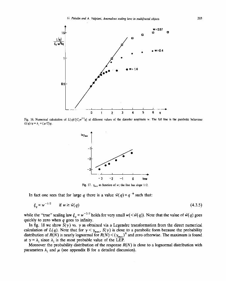
G. Paladin and A. Vulpiani, Anomalousscaling laws in multifracial objects 203
w=0.07
1.5- 0 0 0
L(q) /0
C2w~4q // * w=0.4
/ * *
1•
I./‘ - •
0.5 -
I I I I I
0 1 2 3 4 5 6 q
Fig. 16. Numerical calculation of L(q)I[C2w213q] at different values of the disorder amplitude w. The full line is the parabolicbehaviour
L(q)/q=A,+(j.~/2)q.
lny,,~,
lfl
Fig. 17. 7~I~ as function of w; the line hasslope1/2.
In fact oneseesthat for large q thereis a value ~‘(q) cc q6 such that:
cc w112 if w �; ~‘(q) (4.3.5)
while the “true” scalinglaw cc w213holdsfor very smallw(<v?(q)). Note thatthevalueof ~3(q)goesquickly to zerowhenq goesto infinity.
In fig. 18 we showS(y) vs. y as obtainedvia a Legendretransformationfrom the direct numericalcalculationof L(q). Note that for 7 < Ymax’ S(y) is closeto aparabolicform becausethe probabilitydistributionof R(N) is nearlylognormalfor R(N)< (7maxY”~’andzerootherwise.Themaximumis foundat y = A
1 since A1 is the most probablevalue of the LEP.Moreoverthe probabilitydistribution of the responseR(N) is closeto a lognormaldistribution with
parametersA1 and j.~(seeappendixB for a detaileddiscussion).
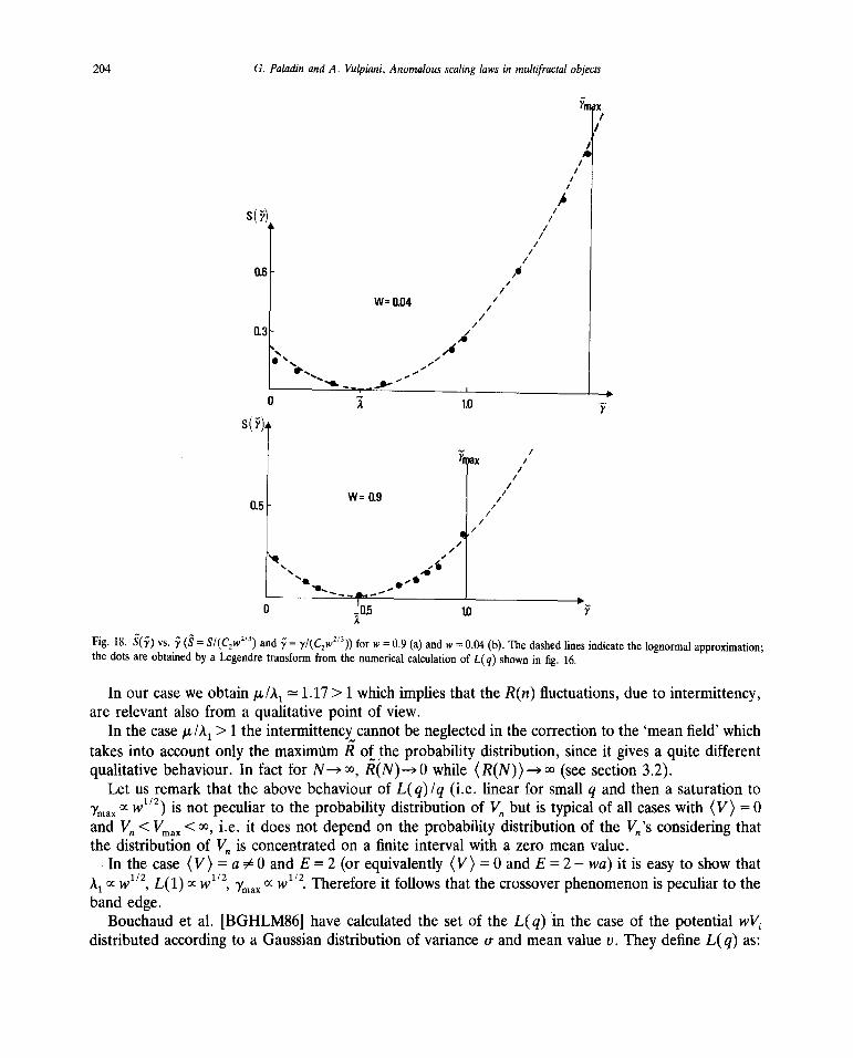
204 G. Paladin andA. Vulpiani, Anomalousscaling laws in multifractal objects
-x/
/
/
‘4,s(~)-
//
/
0.6-/
/
W=0.04 //
/
0.3-
A• •_.
•_.,s.__. ~
O A 1.0 -~
— I/
//
0.5 W= 0.9 ,1
~0 ~D.5 1.0 V
Fig. 18. S(j) vs. Y (~ = S/(C2w213) and ~ = yI(C
2w213)) for w = 0.9 (a) and w = 0.04 (b). The dashedlines indicate the lognormalapproximation;
thedots areobtainedby a Legendretransform from the numericalcalculation of L(q) shown in fig. 16.
In our casewe obtain~ IA1 1.17>1 which impliesthat the R(n) fluctuations,dueto intermittency,
are relevantalso from aqualitativepoint of view.In the casep./A1 > 1 the intermittencycannotbe neglectedin the correctionto the ‘meanfield’ which
takesinto accountonly the maximUm R of the probability distribution,since it gives aquite differentqualitativebehaviour.In fact for N—*cc, R(N)—*0 while (R(N))—÷cc(see section 3.2).
Let us remarkthat the abovebehaviourof L( q) /q (i.e. linear for small q and thena saturationtoYmax cc w
112) is not peculiarto the probability distributionof V~but is typical of all caseswith (V) = 0and 1/,, <Vmax <cc, i.e. it doesnot dependon the probability distribution of the 17,, ‘s consideringthatthe distribution of ~/,, is concentratedon a finite interval with a zero meanvalue.
In the case(V) = a ~0 and E = 2 (or equivalently(V) = 0 andE = 2— wa) it is easyto showthatA
1 cc w~2,L(1) cc ~2, Ymax cc w”2. Thereforeit follows that the crossoverphenomenonis peculiarto the
band edge. -Bouchaudet al. [BGHLM86] havecalculatedthe set of the L( q) in the caseof the potentialwV,
distributedaccordingto a Gaussiandistributionof variancea- and meanvalue v. Theydefine L(q) as:
G. Paladin andA. Vulpiani, Anomalousscaling laws in multifractalobjects 205
1 N q
L(q) = lirn ~ ln((Tr ~A~(i))) (4.3.6)
and they usethe equality:
N q N
K (Tr LI A~(i))) = TrKLJ A~(i)®~)= Tr(A!~)N (4.3.7)
where Ar” denotesthe direct productof Aw® A~®. ® A,,,, q times. One has to estimatetheq q
highesteigenvalueA,, of the 2 x 2 matrix (A,,, ) which can be reducedto a (q + 1) x (q + 1) matrixusingsymmetry considerations[P82].
The calculation inside the bandexceptfor v = 2, gives:
L(q) = A1q + ~q2 for q even (4.3.8)
with A1 = o-I[2v(4 — v)].
At the bandedge v=0, no perturbationtheory hasyet been appliedbut for q = 2 and q =4 oneobtainsrespectively:
A—i = (42)1~ (4.3.9)
wherethe L(2) valueagreeswith the [PVu86]result.Moreover for q integer >2 the a-~
3behaviourwas shown to always hold in the limit of weakdisorder,at differencewith the caseof a boundedpotential where at fixed w a “transition” to thebehaviour(4.3.5) appearsfor q>cjccw116.
We finally recall that somefeaturesof the multifractal natureof one-dimensionallocalizationcan beobtainedby consideringa simplemultiplicative process[PS86,PSTZ87]. Therandommatricesproductproblemis reducedto a scalarproduct (i.e. a randomnumbermultiplication, see appendixB) in theframework of arandomphase-likeapproximation.
4.4. Free energyfluctuationsin spin glasses
In the statisticalmechanicsof disorderedsystemsthe fluctuationsof the free energyamongdifferentreplicascan be regardedas the analogueof the temporalintermittencyin a chaoticsignal. Let us,e.g.,consideraspin model on a D-dimensionallattice with Hamiltonian:
H[{J,1}] = — ~ J11a-,o, (4.4.1)
(‘‘I)
where a, = ±1 is the value of the spin on the- site i and the coupling J,1 is an independent randomvariabledistributedaccordingto a probabilitydistributionP(J,1). Givenacouplingrealization{J~,j,thepartition functionof an N spin systemis the traceof the Boltzmannweightexp(—/3HN):
ZN(/3, {J~~})= ~ exp{—/3HN[{J~J}]}. (4.4.2){~r~}
206 G. Paladin and A. Vulpiani, Anomalousscaling laws in multifractalobjects
The free energyper spin then is in the thermodynamiclimit N—*cc:
F($) = lirn — (ln ZN) = lirn — ~ f P(J,1) dJ,1 ln ZN(/3, {J,1}). (4.4.3)
In orderto computethis quenchedaverageoneusuallyappliesthe so-calledreplicatrick. Onenamelycomputesthe free energyper spin of q non-interactingreplicas:
~(q) = hm — ~— ln(Z~). (4.4.4)
The results obtained at integer positive q are then extrapolated at q = 0:
1- ~Z”~\ NI .
F= lim lim = lim J1(q). (4.4.5)q-O N—’= N/3q q—~O
Even in the meanfield approximationof infinite rangecouplings, this procedureencounteredgreatdifficulties dueto the replicasymmetrybreaking[seee.g. SK75,HP79] which werefinally overcomebythe famousmeanfield Parisi solution [P79].
We do not want to enterinto this problembut justshowhow the ~( q) areinterestingby their own.Indeed, they allow to reconstructthe probability distribution of the partition function among thedifferent realizationswith respectto disorder[DT81, P86].
The multifractal approachcan be easilyextendedto spin glasses.It is sufficient to introducethe freeenergyper spin of a couplingrealization{J~,}of an N-spinsystem:
= — ln ZN(/3, {J,1}). (4.4.6)
In the thermodynamicallimit almost eachsamplehasto havefree energyF and we thusrecovertheselfaveragingof ~
F = ~ N (4.4.7)
This is an ergodicityhypothesissinceweareassumingthat the ensembleaverage(4.4.3)andthe spatialaverage(4.4.6) are equivalent.
In a unidimensionalsystemwith first neighbourinteractionsanduniform field h, we can write thepartition function (4.4.2) as the traceover 2 x 2 randomtransfermatricesproduct.The Hamiltonianisnow H = —~ (J~o,o,~1+ ho~)so that one has:
— N ( exp(f3J,+/3h) exp(—/3J~+/3h) 448ZN—TrM~, Mi_~exp(_/3Jt_/3h) exp(/3J1—/3h) . ( . - )
The maximalLyapunov exponentis thus relatedto the free energywhile the generalizedLyapunovexponentsto the ~( q):
L(q) = —/3 ~(q) q, A1 = —/3F. (4.4.9)
G. Paladin and A. Vulpiani, Anomalousscaling laws in multifraccal objects 207
Derridaet al. [DPV78]have,e.g., found the expressionof A1 in the limit of vanishing temperature forany value of the uniform field if P(J,) is the sum of two delta functions and their method can beextendedto the calculationof L( q).
The readercan identify — I3EN with the LEP ‘y (seedefiniti6n (3.5.5)) whoseprobabilitydistributionis reconstructed by the knowledge of the generalized exponents L(q).
We can however use the multifractal approach without having recourse to the transfer matrixformalism in a generic dimension.
Let us group all the N spin systemrealizationswith free energyin the range[E, E + dE] into thesame subset 11(E), as usual.If we want a finite free energyperspin andper replica~( q), thenwe mustassume that the probability 11(E) that a realization belongs to 11(E) decaysexponentiallywith N forE�F:
H(E)ccexp{—S(E)N} (4.4.10)
where S(E)� 0 andS(F) = 0. The momentsof the partition function can be estimatedas an integralover the spectrum of the possible free energies [Emjn,Emax]
(ZN(/3)”) 11(E)dE exp(—/3EqN). (4.4.11)
We thus have in the limit N—* cc:
q /3 ~~(q) = mn [I3Eq + 5(E)]. (4.4.12)
Let us note that the Oseledectheoremcorrespondsto the self-averaging(4.4.7) as in the previoussection.
Let us conclude with the remark that if the .J~ are bounded(i.e. IJ~JIS C), it is possible to give arough estimate on the minimal value of the free energy Emjn. It is in factgiven by the free energyof thepuresystemJ~, = C for eachcouple of neighboursi, j.
5. Multifractal structures in condensedmatter systems
5.1. General remarks
In this sectionwe briefly review somecritical or critical-like phenomenain the studyof which themultifractal method appearsas a powerful tool. The usual attitude is to assumethat the relevantfeatures of a system near the critical point are determined by a finite number of relevant operators.
It is thereforenaturalto askwhetherthis ideais in agreementor not with theexistenceof anomalousscaling and of multifractal structures.
Fourcadeetal. [FBT86a,FBT86b] haveshownthat the anomalousscalingis compatiblewith a finitenumber of relevantoperatorsevenif an infinite set of irrelevant operators(irrelevant in the usualtechnical senseused in critical phenomena)are also important. They are related to the Renyidimensions d,, with n >0 andgive acompletecharacterizationof the statisticalpropertiesof thesystem.
Let us,e.g., considerthe caseof a latticewhosebondsareoccupiedby a resistorwith probability p
208 G. Paladin andA. Vulpiani, Anomalousscaling laws in multifractal objects
or by an insulator with probability 1 — p. In theserandomresistornetworks,closeto the percolation
thresholdp,~,the measurablequantitiesof interesthavethe form
wherey,~is the powerdissipatedin the branchk. Nowwe define the exponent x,, (analogousto d,,) asfollows:
cc L~ L-*cc (5.1.1)
where (~)EL refers to the averageover the sample realizations,L is the systemsize L ~ ~ andcc (p — p,~)’~is the correlationlength. In analogywith the critical phenomenawe introducethe joint
probability for ~k ~ ~k y~
andwe assumethe following finite-sizescaling behaviour:
~ y~, ~ y~,. . ., ~,L) = Ax0Ax1 - . . p(~y~/A~o,~ ~ , ~IA, LIA) (5.1.2)
whereA is a rescalingparameter.No checkof the scaling (5.1.2)hasappearedyet. Howeverit hasbeennumericallyverified [ARC85]
andin somecasesproved [SW76]that partial distributionfunctions
~ y~/A~,cc, i) = Jud(~y~/L~i)~ y~/L~o,.- cc, i) (5.1.3)
do scaleas predictedby eq. (5.1.2). We remarkthat eq. (5.1.2) implies
((~yfl)tm) ccLrnx,I (5.1.4)
i.e. powers of a given U~= ~ k y~obey to a gap scalingbut different U,, scalein an anomalousway.Onecan see[RTT85]that thereis a relevantoperator,controlledby p — p,~,while thereis aninfinite
setof irrelevantoperatorsbecausex0 — x,, <0 for n >0.
A similar result hasbeenobtainedin a 4,4 theory: aninfinite setof irrelevant operatorsassociatedwith $ dx 4,”(x) is necessaryto give acompletecharacterizationof the distributionfunction of the field4, [FBT86a].
5.2. Multifractal wavefunctionat the localizationthreshold
Wewant here to dicuss further the Anderson model by considering the structure of the wavefunctionat the localization transition. The universal properties near the localization threshold can be investi-
G. Paladin andA. Vulpiani, Anomalousscaling laws in multifractal objects 209
gatedby an expansionin the difference betweenthe spatial dimensionD and the lower criticaldimensionwhich is commonly believed to be two [AALR79]. It was in fact arguedthat even thepresenceof weak disorder inducesa (marginal) localizationof all the quantumstatesof independentelectronsin two dimensions.Wegner[W79,W80] showedhow the localizationproblemcan be handledby meansof c-expansiontechniquesapplied to the non-lineara--model.
He determined[W80,W86] the exponentsof the momentsP,, of thewavefunctionsfor theAndersonlocalization definedas:
P,,(E) = (~4,~(r)~2”~(E- EA))/~(E) (5.2.1)
where~/‘A is the amplitudeof the localizedwavefunctionI A) with energyEA atsite r and,5 is the densityof states.
The averageis takenover realizationsof the disorder.P,, vanishesnearthe mobility edgeE~like:
P,,(E)cc (E — E~)”~cc ~ (5.2.2)
As before,~ is the localization lengthwhich scalesas
~(E) cc (E — ~ (5.2.3)
The value v = 1/c + 0(c3) evaluatedin the c-expansionis often consideredexact [KS83,H83].The critical exponentsin (5.2.2) havebeenobtained[W86]up to the third order in c:
H,,Dv(q—1)— ~“2q
(5.2.4)
~q=q(q_1)[1_f~1 c3(q2_q+l)]+O(c4)
with ~(3)— 1.2020569.Castellaniand Peliti [CP86]relatedthe anomalousscalingof Pq to the multifractal structure of the
wavefunctionnearthe localization threshold.They assumed that just one typical wavefunction 40E gives a significant contributionto the moments
Pq(E) for E—E~.It follows that it is possible to define a coarse grained probability density, ‘a mass’, p.(l) by
integrating ~ over a box A, of size 1:
p~(l)=~ kD~(x)I2dx. (5.2.5)
Its supportis the wholespaceof dimensionD = d0 which is not fractalof course,but can beregardedas
multifractal with respectto the scalingof p,(l).On the otherhand,we can estimatethe momentsP,,(E) for E E~integrating I ~PEIover a box of
size ~ since ‘PE rapidly decaysfor scaleslarger than~:
210 G. Paladin and A. Vulpiani, Anomalousscaling laws in mullzfractalobjects
-11 Ip
Pq(E)=’~ ~ p,(l)~cc(~) . (5.2.7){boxesA~}
Nearthe critical point wecan howeverevaluateP,, by means of the coarse grained probability densityp,(l) becauseof the scaling invariance.
With the standardassumptions,the relevantscalingparameterfor the rescaledsystemmadeof boxesof size 1 is ~Il andone has:
—n Iv
Pq(E) ~ p.(l)” cc (~) . (5.2.7){boxesA,)
A direct comparisonof (5.2.7)with (5.2.6) shows that
4,(q) = d,,~1q= Hq+i/P. (5.2.8)
The singularitiesof the measureI ~(x) 2 dx with respect to the Lebesguemeasurecan then becharacterizedby meansof the Renyi dimensionscomputedwith field theoretical techniques.Onenamelyfinds to fourth order in c:
d,,~1= D — v~(q+ 1) + v~c3 (q3 + 2q2 + 2q + 1). (5.2.9)
Wecan write (5.2.9) using the estimate v~= s + 0(c5) [H83] andnoting D = 2 + c:
dq+i = D1 — + -~ c’~(2q
2 + q3)+ 0(c5) (5.2.10)
where:
= 2 + ~-~- s4 + 0(c5) (5.2.lla)
= c(i — ~ c3) + 0(c5). (5.2.llb)
This result indicatesthat the wavefunctionhasa multifractalstructuresincethe information dimensiondiffers from the space dimension d
0 = D.Weare interested in the three-dimensional case where we have to extrapolate formula (5.2.10) up to
c= 1 to obtain the informationdimension:
d1 2.3. (5.2.12)
Let us recall that 4,(q) is a convexfunction of q (i.e. dq is non-increasing).Moreover,4,(q) is non-decreasingif oneexcludesthe possibilityof negativemeasuresingularitiesa.
At c = 1 we can therefore trust the c-expansion result (5.2.10) only up to q 1.25 corresponding tod125~2.24,see fig. 19.
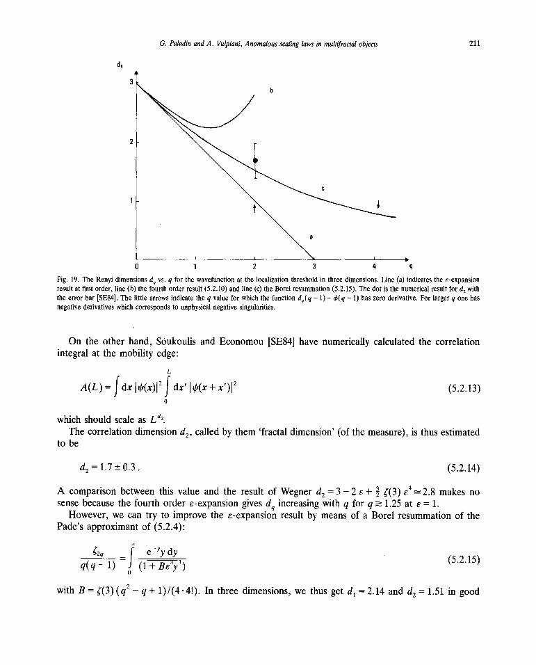
G. Paladin andA. Vulpiani, Anomalousscaling laws in multifractal objects 211
dq
3b
2
C
t
I I
0 1 2 3 4 q
Fig. 19. The Renyi dimensionsdq vs. q for the wavefunctionat the localization thresholdin threedimensions.Line (a) indicatesthe c-expansionresultat first order,line (b) thefourth orderresult(5.2.10)and line (c) theBorel resummation(5.2.15).The dot is thenumericalresultfor d
2 withthe errorbar [SE84].The little arrowsindicatetheq value for which thefunctiond,(q —1) = 4’(q — i) haszeroderivative.For largerq onehasnegativederivatives which correspondsto unphysicalnegativesingularities.
On the other hand,Soukoulis and Economou[SE84]have numerically calculatedthe correlationintegral at the mobility edge:
A(L) = f dx I~(x)I2Jdx’ I~(x+ x~)I2 (5.2.13)
which should scaleas L d2
The correlationdimensiond2, calledby them ‘fractal dimension’(of the measure),is thusestimatedto be
d2 = 1.7±0.3. (5.2.14)
A comparisonbetweenthis value and the result of Wegnerd2 = 3 — 2 c + ~ ~(3)c4 2.8 makes no
sense because the fourth order c-expansion gives d,, increasingwith q for q � 1.25 at e = 1.However, we can try to improve the c-expansionresultby meansof a Borel resummationof the
Pade’sapproximantof (5.2.4):
_____ i e~ydy 52 5
q(q—1) J (1+Bs3y3) ( . .1)
with B = ~(3)(q2— q + 1)I(4 •4!). In three dimensions,we thusget d1 = 2.14 and d2 = 1.51 in good
212 G. Paladin andA. Vulpiani, Anomalousscaling laws in multifracial objects
agreementwith the numericalestimate(5.2.14).Figure 19 showsthe resultsfor the Renyi dimensionsobtained to first order in s, at the fourth order in c (5.2.10) and by the Borel resummation (5.2.15).
In our discussionwe haveimplicitly extendedthe results(5.2.4) for to non-integerq-values.It isthen possible to apply the usual Legendre transformation to obtain either f(a) or H(a) = —f(a) + a
which characterizethe singularitiesa of the measure.It is ratheruseful to write H(a) in powersof D = D1 — a = 2— a + (~(3)I4)c
4+ 0(c5):
H(a) = I [ + c-~-~-~-~-j52 + c2 ñ + O(c4)]. (5.2.16)
Let us stress that a first-order calculation [CP86] gives dq+1 = 2 — cq and the parabolic shape
H(a) = (2 — a)2I(2~s)with D
1 = 2 and ~ = 2c. In this case,the ‘relevant’ (in the information theorysense)part of the critical wavefunctionwould cover a bidimensional structurein any spacedimen-sionality D � 2.
The function H(a) is definedin a boundedrange [amjn>0, amax] as discussedin the first section.Near the critical point, the probability P(a) of finding a box for which p,(l) i” should scalelike:
P(a)cc ~~~(a)
This meansthat at fixed 1, the probability of finding a singularitywhich differs from the informationdimension vanishes as a power of ~as E tendstowardE~,the mobility edge.In thelimit E = E~only thesingularity a = D1 survives.
In this sensewe havea hierarchyof critical exponentsdq in contrastwith usual critical phenomena.The larger is H(a), the lessimportant is the correspondingexponenta. At the top of the hierarchythereis the information dimensionfor which H reachesits minimumvalue H = 0.
5.3. Growth probability distribution in kinetic aggregationprocesses
The diffusion limited aggregatesDLA were introduced by Witten and Sander[WS81]for thedescription of growth phenomena. In this model the growth on a lattice starts from an initial seed. Ateachstepa diffusive particle is releasedfrom infinity. When it strikes the aggregatecluster,it becomespart of the cluster.
It is simple to generatesuch an aggregateon a two-dimensionallattice by a numericalsimulation.One thus obtainsa fractal objectwith DF 1.7 which has a highly ramified structuresince particledeposition is favoured at the tips. This implies practically full screening of the bulk.
The relevant propertiesof these clusters can be characterizedby the site growth probabilitydistribution. We have namely to considerthe probability p(r) dr that a randomwalker lands on theboundaryof the cluster 91’ betweenthe points r and r + dr.
p(r) is the harmonicmeasurewhich can be definedfor the boundary~3I’of the clusteras the normalderivative 3,,g of the Green’s function g(r) for the Laplace equation~g = 0 with the boundaryconditions g(co)= constantandg(aF)= 0. The singularitiesof p(r) were first characterizedby meansofthe multifractal approachby Halseyet al. [HMP86I.The coarsegrainedprobability overa box A, ofsize 1 andcentrer~is:
p~(l) p(r) dr. (5.3.1)
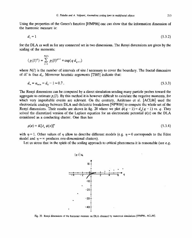
G. Paladin and A. Vulpiani, Anomalousscaling laws in multifractalobjects 213
Using the propertiesof the Green’sfunction [HMP86]onecan showthat the informationdimensionofthe harmonicmeasureis:
d1 = 1 (5.3.2)
for the DLA as well as for anyconnectedsetin two dimensions.The Renyi dimensionsaregivenby thescalingof the moments:
N(1)
(~(l)~)= ~ ccexp(qdq+i)
whereN(l) is the number of intervals of size 1 necessaryto coverthe boundary.The fractal dimensionof ~[‘ is thus d0. Moreoverheuristicarguments[TS85]indicatethat:
d,~amjndo~l~0.7. (5.3.3)
The Renyi dimensionscan becomputedby a direct simulationsendingmanyparticleprobestowardtheaggregateto estimatep,(1). By this method it is however difficult to calculate the negative moments, forwhich very improbable events are relevant. On the contrary, Amitrano et al. [ACL86] used theelectrostaticanalogybetweenDLA anddielectricbreakdown[NPW84]to computethe wholesetof theRenyi dimensions.Their results areshown in fig. 20 wherewe plot 4,(q — 1) = dq(q— 1) vs. q. Theysolved the discretizedversion of the Laplaceequationfor an electrostaticpotential~‘(x)on the DLAconsideredas a conductingcluster. One thushas
p(x) = K[o,, 4,(x)]~1 (5.3.4)
with ~ = 1. Other valuesof i~allow to describedifferent models(e.g. i~= 0 correspondsto the Edenthodeland ~ = cc producesone-dimensionalclusters).
Let usstressthat in the spirit of the scalingapproachto critical phenomenait is reasonable(seee.g.
(q-1)dq -
10
I I I I ~ I I I-4 -2 2 4 6 q
-10
-20
—30-
-40
Fig. 20. Renyi dimensionsof the harmonicmeasureon DLA obtainedby numericalsimulations[HMP86,ACI..86].
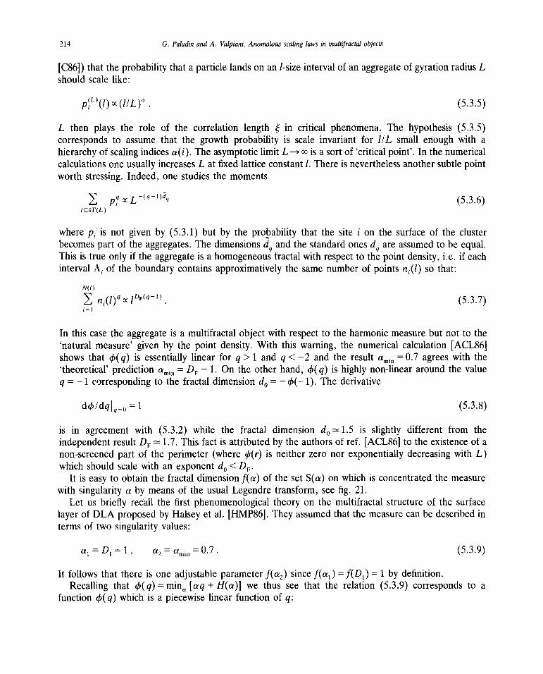
214 G. Paladin and A. Vulpiani, Anomalousscaling laws in multifractal objects
[C86])that theprobability that aparticlelandson an 1-sizeinterval of an aggregateof gyrationradiusLshould scale like:
(L)(l)(l/L)a - (5.3.5)
L then plays the role of the correlation length ~ in critical phenomena.The hypothesis (5.3.5)correspondsto assumethat the growth probability is scale invariant for lIL small enoughwith ahierarchyof scalingindices a(i). Theasymptoticlimit L —~ cc is asort of ‘critical point’. In thenumericalcalculationsoneusuallyincreasesL atfixed latticeconstant1. Thereis neverthelessanothersubtlepointworth stressing.Indeed,one studiesthe moments
~ p~cc (5.3.6)iESF(L)
wherep, is not given by (5.3.1) but by the probability that the site i on the surface of the clusterbecomespart of the aggregates.The dimensionsdq andthe standardonesdq are assumedto be equal.This is true only if the aggregateis ahomogeneousfractal with respectto the point density,i.e. if eachinterval A, of the boundarycontainsapproximativelythe samenumberof pointsn~(l)so that:
N(l)
~ n,(l)’ cc ~DF(~_1) - (5.3.7)
In this casethe aggregateis a multifractal object with respectto the harmonicmeasurebut not to the‘natural measure’given by the point density.With this warning, the numericalcalculation[ACL86]showsthat q5(q) is essentiallylinear for q> 1 and q < —2 and the result amj,, = 0.7 agreeswith the‘theoretical’ predictionamjn = DF — 1. On the otherhand, 4,(q) is highly non-lineararoundthe valueq = —1 correspondingto the fractal dimensiond0 = — 4,(—1). The derivative
d4,/dq~,,0= 1 (5.3.8)
is in agreementwith (5.3.2) while the fractal dimension d0 1.5 is slightly different from theindependentresultDF 1.7. This fact is attributedby the authorsof ref. [ACL86] to the existenceof anon-screenedpart of the perimeter(where l/J(r) is neitherzero nor exponentiallydecreasingwith L)which should scalewith an exponentd0 < DF.
It is easyto obtainthe fractal dimensionf(a) of the set S(a) on which is concentrated the measurewith singularitya by meansof the usual Legendretransform, seefig. 21.
Let us briefly recall the first phenomenologicaltheory on the multifractal structureof the surfacelayerof DLA proposedby Halseyet al. [HMP86].They assumedthat the measurecan be describedintermsof two singularity values:
a1D1’l, a2 amjnO.7. (5.3.9)
It follows that thereis one adjustableparameterf(a2) sincef(a,) = f(D1) = 1 by definition.
Recalling that qS(q) = mina [aq + H(a)] we thus see that the relation (5.3.9) corresponds to afunction çb( q) which is a piecewiselinear function of q:
G. Paladin and A. Vulpiani, Anomalousscaling laws in multifractal objects 215
f(a)
2
1 •~ ••S
0• S
•
1- S
2 , I I I I I I0 2 4 6 8 10 a
Fig. 21. f(a) vs. a for DLA obtainedby a Legendretransform of thedq’5 shownin fig. 20.
Jçb(q)=a1q+H(a1)—D1qq, for q<q~ 53 0~4,(q)=a2 q+H(a2)—(D~—1)(q+1)—f(a2), for q>q ( . .1)
whereH(D1) =0 and H(a2) =f(a2) — a2.The knowledgeof q,~is equivalentto that of H(a2) since by matchingthe two linesone gets:
q~—H(a2)I(1a2). (5.3.11)
Theseresults agreequite well with the direct calculation of the momentsfor positive q � 1 using thevaluef(a2= 0.71)= 0.42, i.e. q, = 0.74. On the otherhandthe formula(5.3.10)is inconsistentwith theresultfor the fractal dimensionsince it impliesDF = — 4,(— 1) = 1 which is muchsmallerthanthe valueDF = 1.71 assumedfor estimatinga2.
5.4. Multifractality in percolation
The critical behaviourof randomresistornetworksis a percolationproblemwhich can be studiedbymeansof the multifractal approach[ARC85, RTBT85].
Let usconsidera latticeof size L whereeachbondis conductingwith probabilityp or insulating withprobability 1 — p. In the limit of infinite L thereis a percolationthresholdp,~abovewhich thereis aninfinite cluster of conductingbonds.
At the critical pointp~oneisolatesthe setof bondscarryinga non-zerocurrent from the restof theinfinite cluster. This set is called the backbone and is a fractal object with dimension:
D~,BB)=lnnBB(L)/ln L for L—~cc (5.4.1)
wherenBB (L) is herethe numberof bondsbelonging to the backboneof a systemof size L.Let us stressthat this is not the box-countingdefinition (0.1). The backboneis made of singly
connectedbonds (links) and of multiply connectedbonds (blobs) in a selfsimilar way. The fractaldimensionof the setof the links is 1 /v wherev is the connectednesslength exponent[C81].
Let usnow considerthe backboneas a randomresistornetworkeachbond havinga unit resistance.A unit voltageis thenapplied to the oppositeboundariesof a box containingthe percolatingcluster.
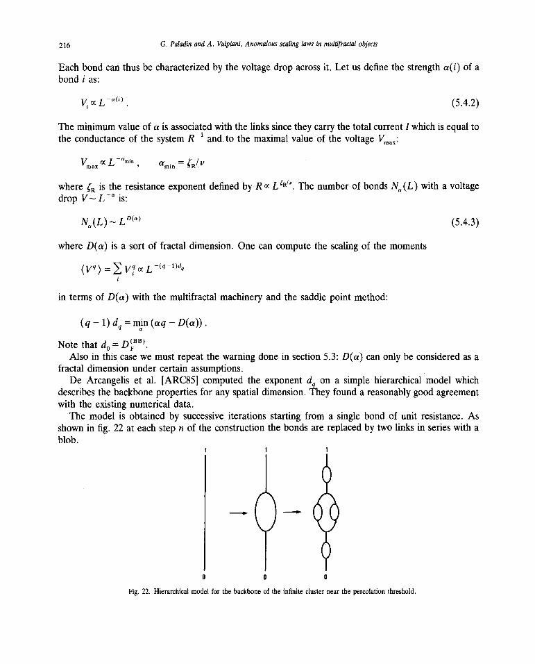
216 G. Paladin and A. Vulpiani, Anomalousscaling laws in multifractalobjects
Eachbond can thusbecharacterizedby the voltage drop acrossit. Let us definethe strengtha(i) of abond i as:
VccL~’~. (5.4.2)
The minimumvalue of a is associatedwith thelinks sincetheycarrythe total currentI whichis equaltothe conductanceof the systemR ~ and.to the maximalvalueof the voltage Vmax:
Vmax cc L~m11. , amjn =
where ~R is the resistance exponent defined by Rcc L “v”. The numberof bondsNa(L) with avoltagedrop V—L~’is:
N(L) —~LD~ (5.4.3)
whereD(a) is a sort of fractal dimension. One can compute the scaling of the moments
(1/”) ~
in terms of D(a) with the multifractal machineryand the saddlepoint method:
(q — 1) dq = mm (aq— D(a)).
Note that d0 = D~BB).Also in this case we must repeat the warning done in section 5.3: D(a) can only be consideredas a
fractal dimensionundercertainassumptions.De Arcangeliset al. [ARC85] computedthe exponentd,, on a simple hierarchicalmodel which
describesthe backbonepropertiesfor anyspatialdimension.They founda reasonablygood agreementwith the existingnumericaldata.
The model is obtainedby successiveiterationsstarting from a single bond of unit resistance.Asshownin fig. 22 at each step n of the constructionthe bondsarereplacedby two links in serieswith ablob.
Fig. 22. Hierarchicalmodel for thebackboneof the infinite clusternearthepercolationthreshold.
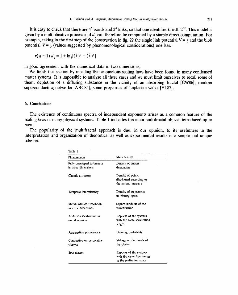
G. Paladin and A. Vulpiani, Anomalousscaling laws in multifractal objects 217
It is easyto checkthat thereare4” bondsand2” links, sothat oneidentifiesL with 2”~.Thismodelisgivenby a multiplicativeprocessanddq can thereforebe computedby asimpledirect computation.Forexample,takingin thefirst stepof the constructionin fig. 22 the single link potentialV= ~andtheblobpotentialV= ~ (valuessuggestedby phenomenologicalconsiderations)one has:
v(q —1) dq = 1 +ln2[(~)” + (~y’]
in good agreement with the numerical data in two dimensions.We finish this sectionby recalling thatanomalousscaling laws havebeenfound in manycondensed
matter systems.It is impossibleto analyseall thesecasesandwe must limit ourselvesto recall someofthem: depletionof a diffusing substancein the vicinity of an absorbing fractal [CW86], randomsuperconductingnetworks [ARC85J,somepropertiesof Laplacianwalks [EL87].
6. Conclusions
The existenceof continuousspectraof independentexponentsarisesas a commonfeature of thescalinglaws in manyphysicalsystems.Table 1 indicatesthe main multifractal objectsintroducedup tonow.
The popularity of the multifractal approachis due, in our opinion, to its usefulnessin theinterpretationand organizationof theoreticalas well as experimentalresultsin a simple and uniquescheme.
Table 1
Phenomenon Mass density
Fully developedturbulence Densityof energyin threedimensions dissipation
Chaoticattractors Densityof pointsdistributedaccordingtothe natural measure
Temporal intermittency Density of trajectories
in ‘history’ space
Metal—insulatortransition Squaremodulusof thein 2 + a dimensions wavefunction
Andersonlocalizationin Replicasof the systemsone dimension with thesamelocalization
length
Aggregationphenomena Growing probability
Conductionon percolative Voltage on the bondsofclusters thecluster
Spin glasses Replicasof the systemswith thesamefree energyin the realizationspace
218 G. Paladin andA. Vulpiani, Anomalousscaling laws in multifractal objects
However, one mustusepropertechniquesfor eachparticularsituationin order to reacha deeperunderstanding of a phenomenon. A typical example is given by the Anderson localization in onedimensionwherethe calculationof the generalizedexponentshavebeendonefollowing somemethodsdevelopedin the context of disorderedsystems[BGHLM86, PS86,PV87b]. The oppositesituationisfully-developedturbulencewhereatheoryon the structureof theNavierStokesequationsingularitiesisstill far from beingformulated. Nevertheless,the analysisin termsof multifractalsis a first useful tooland allows to give a qualitativedescriptionby meansof phenomenologicalmodels.
We think that one of the most interesting future developments will be given by understanding thelink betweentherenormalizationgroupandgeneralizedexponents.An openproblemis the consistenceof the usualscalingwith a finite numberof relevantoperatorsandmultifractality. Some authorshaveshownthat the two aspectsarecompatibleatleast in somecases[FBT86a,FBT86b]. Moreoverthereisnot yet a clearcomprehensionof the mechanismswhich leadto ‘phasetransitions’ (in the generalizedexponentsvarying the moment order) which have been numerically observedin some dynamicalsystemsand aggregates[BP87b,BGP87, ACL86].
Appendix A. The Kolmogorov—Obukhov lognormal model for intermittency in turbulence
Kolmogorov [K62]and Obukhov [062] modified the K41 theory assigninga key role to the statisticsof the spatial distributionof the energydensitydissipationin order to take into accountsomeof theearly evidenceon small-scale intermittency. Essentially in the new modified theory K62 the firsthypothesisof K41 (see section 2.2) is replacedby assumingthat in the range r ~ L the n-variateprobability distributionof u(x + r) — u(x) only dependson ~~(r)= (1 1r3) $A(r) c(y) d3y, r and ii.
The secondhypothesisremainsthe sameone as in K41.Evidently thesetwo hypothesesare quite generaland common to all phenomenologicalcascade
models. To obtain explicit resultsone needsfurther assumptionson the statisticsof c(x), of course.Kolmogorovand Obukhovsupposedthat ~(r) is distributed according to a lognormal in the range
r~r<<L.By dimensional analysis the first two hypotheses give for structure functions:
(I~V(r)Ir~3(~(rY’3). (A.1)
Note that (A. 1) holdsalsofor fractal or multifractal models.Accordingto the third hypothesison thelognormaldistribution, one has[GY67]:
(IAV(r)I~)— r~’31~83’~ (A.2)
i.e.
~ =pf3+(lIl8)p~p(3—p) (A.3)
where ~t is given by the fluctuationsof ~~(r):
= ln(L/r) ((ln ~(r) - (ln ~(r)))2). (A.4)
G. Paladin and A. Vulpiani, Anomalousscaling laws in multifractal objects 219
Kolmogorov and Obukhovpostulatedthe lognormaldistributionwithout anyjustification. It is howevernot difficult to introduce an argumentfor it. We briefly repeatthe derivationdue to Gurvich andYaglom [GY67]. Let uscall c,, the quantity ~ (rn) with r,, = 2 “L, we thenobtain c,, as the productofindependentrandomvariables
c,,e0fl’Pt, ~e~/c1_1. (A.5)
Taking the logarithm of (A.5) one has
lnc,,=lns0+~lnç~. (A.6)
Assumingthat all the variablesln ~ havefinite meanvalueand finite variance(meaningthat the event= 0 hasprobabilityzero)we can apply for large n (r ~gL) the central limit theorem.c,, is therefore
distributedaccordingto a lognormal characterizedby two parameters:
1 1 2
ln(LIr) (ln c,,) and ln(L/r) ((ln c~— (ln c,,)) )
Since (ca) must dependon n, becauseof the constancyof the forward energytransferrate,just arelevantparametersurvives:the variancegiven by (A.4).
Weremark that in the Gurvich—Yaglom derivation there is the basic assumption that ‘P~ vanishes withzero probability. This hypothesisis not madein the fractal (or multifractal) model where therearecubeswith c~= 0 (non-activefluid) [N69, N70, NS64,M74, FSN78,FP85,BPPV84]. This is the mostremarkabledifferencebetweenthe two approaches.
Let us notethat, at least formally, the lognormalmodel is a limiting caseof the multifractal one,assuming a parabolic form for d(h) with a maximum at DF 3 and no restrictionon the possible hvalues.OnethenobtainsDF = 3, D~= DF — ~/2 = 3 — ~t/2, D* DF — = 3 — j~.The energydissipa-tion is concentratedon a three-dimensionalsupportwhich is thereforenot fractal.All thefluid is activebut the ‘measure’given by s(r) is fractal since D1 <3.
in eq. (A.3) hasa parabolicform with a maximumatp” = ~(2+ p~)//2and becomesnegativefor largevaluesof p.
This odd featureis due to the fact that the lognormal model gives no restrictionson the possiblevaluesof s,,. This is clearlyan unphysicalfeatureof the model. Indeed,we haveseenthat plausiblebounds exist for the values of the singularities h (and thereforefor c,,).
The lognormaldistribution,however,is a good approximationfor a largeclassof phenomenabut itgives uncorrectvaluesfor the moments(seeappendixB), since theygrow too rapidly with p and thusviolate the Carleman’scriterion [C22]which hasto be satisfiedfor determininga probability distribu-tion from its moments.This leadsto unphysicalconsequences.If it is not possible to determinetheprobability distributionby momentsof aquantitysatisfyingsomeevolutionequations,thenthe initialvaluesof all the momentsdo not allow to determineuniquely the valuesof the momentsat futuretimes. Orszag [070b] showedthat the non-uniquenessof the moment values at positive times iscompatiblewith the uniquenessof the solution of the evolutionequations.
220 G. Paladin andA. Vulpiani, Anomalousscaling laws in multifractal objects
Appendix B. Multiplicative processesandlognormalapproximation
Multiplicative processesarethe simplestway to get anapproximatedescriptionof multifractals.Letus recall the random/3 -model for turbulence(section2.3) or its equivalentfor chaoticattractors[PV84,BPPV84], the responsefunction for temporalintermittency(section3) or randommatrices(section4).In this appendixwe briefly discussthe multiplicative processesand the lognormalapproximationin ageneralcontext.
Let usconsideravariablex,, given by a productof n ~ 1 random variables:
x,, = [I a, (B.1)
wherethe a’s arepositiveindependentrandomvariablesdistributedaccordingto the samedistributionof probability laws. Moreoverwe assumethat
amjn < a, <amax. (B.2)
The probability distributionof x,, is close to the lognormal distribution:
exp[—(lnx~— An)2I(2~n)]P(xfl)=~PLN(xfl)= 1/2 (B.3)
x,,(2i~n)
whereA and ~ aregiven by
A = ! = {ln a}
and
= ~- (ln x,, — fjj~)2= {(ln a — {ln a})2},
where~ standsfor the averageon different realizations[a1,. . . a,,] and { ( )} meansaveragegiven by
the probability distribution of a: { ( )} = f P(a) (.) da.Note that the logarithm of x,, is given by a sumof independentrandomvariables
lnx~=~lna~. (B.4)
Becauseof the inequalities(B.2)andthe independenceof thea. we can apply the central limit theorem.Thereforethe probability distributionof the variabley,, = ln x,, is closeto aGaussianwith meanvaluenA and variancenj~.Equation(B.3) follows from a changeof variables.
In spiteof the fact that the lognormaldistributionis a goodapproximation,its momentsarenot closeto the right ones.
Using eq. (B.3) one has
G. Paladin and A. Vulpiani,Anomalousscaling laws in multifractal objects 221
x~=f x,,” PLN(xfl) dx~ exp{ng~~(q)}
with
g~~(q)=Aq + ~jsq2. (B.5)
It is trivial to seethat (B.5) cannotbe valid for largeq. Indeedone cancomputex,, directly by (B.1):
~=e”~”-) withg(q)=ln{a”} (B.6)
and becauseof (B.2) one has:
q ln(amjn) <g(q) < q ln(amax). (B.7)
Equation (B.5) is not thereforea good approximation for large q. On the contrary, writing x,, =
exp(q lnx~)andexpandingin seriesto the secondorder in q, we see thatfor smallq, g(q) g~~(q).This apparentparadox(a probabilitydistributioncloseto the lognormalwhosemomentsdo not follow(B .5)) is related to the fact that the momentsof the lognormal distributiongrow too fast [C22, O70b,M72].
Without invoking complexmathematicalargumentsonecan convinceoneselfthat the origin of thetrouble resides in the tail of ~LN (x~).Indeed, the true probability distribution P(x~)is zero for
> (a,,,,,1,)~,while for largeq the greatestcontributionsto J~°x,,” PLN(xfl) dx,, comefrom aregion where
P(x,,)= 0. This becomesevident by computingthe valuei~”~for which x~”PLN(xfl) takesits maximum.Onein fact finds for largeq
exp(const.~,~. q) ~. (amax)”
We concludeby noting againthata lognormalapproximationfor moderatevaluesof q (i.e. aparabolicshapeof f(a) for aaroundD1) is rathergood,while for largeq boundslike (B.2) haveto be takenintoaccount.
For exampleif we repeatthe considerationsof this appendixfor fully developedturbulence,wegetan approximateexpressionfor ~,sincethe random/3-modelinvolvesamultiplicative processfor i(r).
Let us remind (eq. 2.3.15)that in the random/3-modelone has
(I~V(r,,)V) r’3{fl /3(1P/3)}
Onethereforeobtains,consideringthe lognormal approximationfor the variable fl~ /3~:
~ ~p/3 + D,(1 —p13)+ (~/2)(1—p13)2 (B.8)
for I p —31 not very large.Note that in (B.8) therearetwo independentprametersD
1 and~swhile only oneis involved in K62.
222 G. Paladin and A. Vulpiani, Anomalousscaling laws in multifractal objects
Wehave in fact considered the multiplicative process on the fractal and the constraint ~ = 1 is imposedautomatically by the model.
Acknowledgements
We thank Giorgio Parisi for his constantandwarm interestin our work as well as for enlighteningsuggestions.
Weenjoyed many exchanges of ideas and the friendly help of R. Benzi, C. Castellani,A. Crisanti,M. Mezardand L. Peliti.
We also acknowledge valuable and interesting discussions with C. Amitrano, L. de Arcangelis, R.Badii, J.P. Bouchaud,A. Coniglio, F. De Pasquale,C. Di Castro, C. Evertsz, A. Georges,P.Grassberger,P. Le Doussal,L. Pietronero,A. Politi andP. Siebesma.Particularthanksaredueto A.Crisanti,B. Fourcadeand A.M. Tremblayfor a critical readingof the manuscript.
References
[AALR79]E. Abrahams,P.w. Anderson,D.C. Licciardelloand TV. Ramakrishan,Phys. Rev.Lett. 42 (1979) 673.[ACL86] C. Amitrano, A. Coniglio and F. di Liberto, Phys.Rev. Lett. 57 (1986) 1016.
[A58] P.W. Anderson,Phys.Rev. 109 (1958) 1492.[AL77j J.C. Andreand M. Lesieur,J. Fluid Mech. 81(1977)187.
[AGHA84] F. Anselmet,Y. Gagne,E.J. Hopfingerand A.R. Antonia, J. Fluid Mech. 140 (1984) 63.
IARC85] L. de Arcangelis,S. RednerandA. Coniglio, Phys.Rev. B31 (1985) 4725.LBBS84] A. Babiano,C. Basdevantand R. Sadourny,CR. Acad. Sci. ParisB299 (1984) 495.
[BP84]R. Badii and A. Politi, Phys. Rev.Lett. 52 (1984) 1661.[BP851R. Badii and A. Politi, J. Stat. Phys.40 (1985) 725.
[BP87alR. Badii andA. Politi, Phys. Rev. A35 (1987) 1288.[BP87blR. Badii andA. Politi, Phys. Scr.35(1987)243.
[BGP87IR. Badii, P. Grassbergerand A. Politi, unpublished(1987).
[BR56j 1. Balatoni and A. Renyi, Pub. Math. Inst. HungarianAcad. Sc. 1 (1956) 9.[BLSB81]C. Basdevant,B. Legras,R. SadournyandM. Beland, J. Atmos. Sci. 38 (1981) 2305.
[BT49] G.K. Batchelor and A.A. Townsend,Proc. Roy. Soc. A199 (1949) 238.
1B691 G.K. Batchelor, Phys.Fluids 12 (1969) S233.[BGS76]G. Benettin, L. Galganiand J.M. Strelcyn, Phys. Rev.A14 (1976) 2338.
[BGGS8O]G. Benettin, L. Galgani, A. Giorgilli and J.M. Strelcyn,Meccanica15 (1980) 9 and 21.[B84l G. Benettin, Physica13D (1984) 211.
[BPPV84]R. Benzi, G. Paladin, G. Parisi and A. Vulpiani, J. Phys. All (1984) 3521.[BPPV85]R. Benzi,G. Paladin, G. Parisi and A. Vulpiani, J. Phys.A18 (1985) 2157 and 3281.[BPPV86]R. Benzi,G. Paladin, G. Parisi and A. Vulpiani, J. Phys.A19 (1986) 823.
[BPPSV86]R. Benzi,G. Paladin, S. Patarnello,P. SantangeloandA. Vulpiani, J. Phys.A19 (1986) 3771.(B77] MV. Berry, J. Phys. AlO (1977) 2061.[B82] MV. Berry, J. Phys.A15 (1982) 2735.
[BPTV87ID. Bessis,G. Paladin, G. Turchettiand S. Vaienti (1987), unpublished.[BGHLM86] J.P. Bouchaud,A. Georges,D. Hansel,P. Le Doussaland J.M. Maillard, J. Phys. A19 (1986) L1145.
[B75] R. Bowen, Equilibrium Statesand the Ergodic Theory of AnosovDiffeomorphisms. Lect. Notesin Math. 470 (Springer Verlag,Berlin, 1975).
[B79] R. Bowen,Pubi. Math. IHES 50 (1979) 11.[BMONMF84]ME. Brachet,D. Meiron, S. Orszag,B. Nickel, R. Morf and U. Frisch, J. Stat. Phys. 34 (1984)1049.
[CP861C. Castellaniand L. Peliti, J. Phys. A19 (1986) L429.1C85] J.P. Caputo,in: Advancesin nonlineardynamicsandstochasticprocesses,eds.R. Livi and A. Politi (world Scientific PubI., 1985)
p. 171.[C22l T. Carleman,CR. Acad. Sc. Paris174 (1922) 1680.
[CW86]ME. Catesand TA. Witten, Phys. Rev. Lett. 56 (1986) 2497.
G. Paladin and A. Vulpiani,Anomalousscaling laws in multifractalobjects 223
1C691 W.J. Cocke, Phys.Fluids 12 (1969) 2488.[CP85JA. CohenandI. Procaccia,Phys.Rev. A31 (1985) 1872.[C81JA. Coniglio, Phys. Rev. Lett. 46 (1981) 250.(C86] A. Coniglio, Physica140A (1986) 51.
[CFMT85]P. Costantin,C. Foias, OP. Manley andR. Teman,J. Fluid Mech. 150 (1985) 427.[C62]S. Corrsin, Phys. Fluids 5 (1962) 130.
[CPV87]A. Crisanti,G. Paladin and A. Vulpiani, preprint (1987).[CFU82]J.P. Crutchfield, J.D. Farmer and BA. Huberman,Phys. Reports92 (1982) 45.[DLS85JF. Delyon, Y. Levy and B. Souillard, Phys. Rev. Lett. 55 (1985) 618.[DG84I B. DerridaandE. Gardner,J. Phys. (Paris)45 (1984) 1283.
fDPV78] B. Derrida, Y. Pomeauand 1. Vannimenus,J. Phys. Cli (1978) 4749.[DT811B. Derrida andG. Toulouse,1981 Proc. 6th Brazilian Symp. on TheoreticalPhysics(ed. CNPQ).
1EP861 J.P. Eckmannand I. Procaccia,Phys. Rev. A34 (1986) 659.[ER85] J.P. Eckmannand D. Ruelle,Rev. Mod. Phys. 57 (1985) 617.[ELS7IC. EvertszandJ.W. Lykiema, Phys.Rev. LetI. 58 (1987) 397.
FF821 ID. Farmer, Z. Naturforsch.A37 (1982) 1304.[F87]MI. Feigenbaum,J. Stat. Phys. 46 (1987) 919.[F71]W. Feller, An Introductionto Probability Theory andits Applicationsvol. 2 (New York, Wiley, 1971).
[FH63]RH. Feynmanand AR. Hibbs, QuantumMechanicsand PathIntegrals(Gordonand Breach,1963).[FBT86aIB. Fourcade,P. Bretonand A.M.S. Tremblay,Ann. Sc. Math. Quebec,in press.[FBT86bJB. Fourcade,P. Breton and A.M.S. Tremblay, preprint (1986).
[F76l U. Frisch, in: Problemsof stellarconvection,eds. E.A. Spiegel andJ.P. Zahn (Springer,1976)p. 325.[FP85]U. Frisch andG. Parisi, in: Turbulenceandpredictabilityof geophysicalflows andclimaticdynamics,eds.N. Ghil, R. BenziandG.
Parisi (North-Holland, 1985).
[F5N78]U. Frisch, P. Sulem and M. Nelkin, J. Fluid Mech. 87 (1978) 719.FF831 H. Fujisaka, Progr. Theor. Phys. 70 (1983) 1264.
[GM72] C.H. Gibsonand P.J. Masiello, in: StatisticalModels andTurbulence,eds. M. Rosenblattand C. Van Atta, Lecture Notes inPhysics12 (Springer,Berlin, 1972) p. 427.
[G78l R. Graham,in: StochasticProcessesin NonequilibriumSystems,eds. L. Gamdo,P. Seglar and P.J. Shepherd(Springer, 1978)p. 82.
fG83] P. Grassberger,Phys. Lett. A97 (1983) 227.[G86ajP. Grassberger,private communicationto the authors(1986).[G86b]P. Grassberger,in: Chaos,ed. A.V. Holden (ManchesterUniv. Press,1986)p. 291.
[GP83a]P. Grassbergerand I. Procaccia,Phys. Rev. Lett. 50 (1983) 346.[GP83b]P. Grassbergerand I. Procaccia,Phys. Rev.A28 (1983) 2591.[GY67]AS. Gurvich and A.M. Yaglom, Phys. Fluids 10 (1967) S59.
[HJKPS86]T.C. Halsey,M.H. Jensen,L.P. Kadanoff, L. Procacciaand B.I. Shraiman,Phys. Rev.A33 (1986)1141;A34 (1986) 1601.[HMP86]T.C. Halsey, P. Meakin and I. Procaccia,Phys. Rev. Lett. 56 (1986) 854.
[H19l F. Hausdorff, MathematischeAnnalen 79 (1919) 157.(HP79] J.L. van Hemmenand R.G. Palmer,J. Phys. A12 (1979) 563.
[HP83a]H.G.E. Hentscheland I. Procaccia,PhysicaD8 (1983) 435.[HP83b]H.G.E.Hentscheland I. Procaccia,Phys. Rev.A27 (1983) 1266.
[H76] M. Henon, Comm. Math.Phys. 81(1976)229.[HH64] M. Henon andC. Heiles,Astron. J. 69 (1964) 73.
[H83] S. Hikami, NucI. Phys.B215 (1983) 555.[JKLPS85IM.H. Jensen,L.P. Kadanoff, A. Libchaber,I. Procacciaand I. Stavans,Phys. Rev.Lett. 55 (1985) 2798.
[K86l L.P. Kadanoff,J. Stat. Phys.43(1986)395.[K76] J.P. Kahane,in: TurbulenceandNavier—Stokesequation,ed. R. Teman,Lecture Notes in Mathematics565 (springer,Berlin,
1976)p. 94.[KT8O]T. Kai andK. Tomita, Progr. Theor. Phys. 64 (1980) 1532.[KY78]J.L. Kaplan and l.A. Yorke, Lecture Notesin Math.vol. 730 (Springer-Verlag,Berlin, 1978) p. 204.
[K57] A.Ya. Khinchin, Mathematicalfoundationsof informationtheory(Dover, N.Y., 1957).[K41] AN. Kolmogorov, DokI. Akad. Nauk SSSR30 (1941) 299.[K621AN. Kolmogorov,J. Fluid Mech. 13 (1962) 82.
fK67] RH. Kraichnan, Phys. Fluids 10 (1967) 1417.[K74]RH. Kraichnan, J. Fluid Mech. 63 (1974) 305.[K85l RH. Kraichnan, Phys. Fluids 28 (1985) 10.
jKM8O] RH. Kraichnan and D. Montgomery,Rep. Progr. Phys. 43(1980)547.
224 G. Paladin and A. Vulpiani, Anomalousscaling lawsin multifractal objects
[K583]H. Kunz andB. Souillard, J. PhysiqueLett. 44 (1983) 2503.[KC71] A.Y. Kuo and S. Corrsin, J. Fluid Mech. 50 (1971) 285.
[KC72I A.Y. Kuo and S. Corrsin, J. Fluid Mech. 56 (1972) 447.[LL71] D. LandauandL. Lifschitz, Mecaniquedes Fluides(MIR, Moscow,1971).
[LPC87]J. Lebowitz, A. Porzio andP. Collet, J. Stat. Phys. 47 (1987) 609.[L811F. Ledrappier,Comm. Math. Phys.81(1981)229.
[LM85] F. LedrappierandM. Misiurewicz, J. Ergod. Theory Dyn. Syst. 5 (1985) 595.[L73] D.C. Leslie,Developmentsin theTheory of Turbulence(ClarendonPress,Oxford, 1973).
[LL83] Al. LiechtenbergandMA. Liebermann,Regularand StochasticMotion (SpringerVerlag, Berlin, 1983).[L63] EN. Lorenz, J. Atmos. Sc. 20 (1963) 130.[Loll Lyapunov, Ann. Math.Studies(1907) 17 (Princeton,1947).
[MADB83] B. Mairaison, P. Atten, P. Bergeand M. Dubois, I. Phys.Lett. 44 (1983) L897 and L902.[M72] B.B. Mandelbrot, in: StatisticalModels and Turbulence,eds. M. Rosenblattand C. Van Atta, Lecture Notes in Physics12
(Springer,Berlin, 1972) p. 333.[M74] B.B. Mandelbrot, J. Fluid Mech. 62 (1974) 331.
[M76a1B.B. Mandelbrot, CR. Acad. Sc. Paris A282 (1976) 119.[M76b1B.B. Mandelbrot,in: Turbulenceand Navier—Stokesequation,ed.R. Teman,LectureNotesin Mathematics565 (Springer,Berlin,
1976) p. 121.
[M82] B.B. Mandelbrot,The fractal geometryof nature(Freeman,1982).[MR821GA. McCreadieandG. Rowlands,Phys. Lett. A91 (1982) 146.
[M84) IC. McWilliams, J. Fluid Mech. 146 (1984) 21.[MCS861P. Meakin, A. Coniglio andHE. Stanley, Phys.Rev. A34 (1986) 3325.
[M861J. Melrose, I. Phys. A19 (1986) 821.[MW85] A. Mielke and F. Wagner,Z. Phys. B62 (1985) 1.[MY75]AS. Monin and AM. Yaglom,StatisticalFluid MechanicsVol. 2 (MIT Press,CambridgeMass.,1975).
[MOF8O]RH. Morf, S.A. Orszagand U. Frisch, Phys. Rev.Lett. 44 (1980) 572.[NN85]T. NakanoandM. Nelkin, Phys. Rev. 31A (1985) 1980.
[N86] T. Nakano,Progr. Theor. Phys.75(1986)1295.[NPW84]L. Niemeyer,L. Pietroneroand H.J. Wiesman,Phys.Rev. Lett. 52 (1984) 1033.
[N69] E.A. Novikov, Dokl. Akad. Nauk SSSR184 (1969) 1072.[N701E.A. Novikov, Prikl. Mat. Mekh. 35 (1970) 266.
[NS641E.A. Novikov and R.W. Stewart,Izv. Akad. Nauk SSSR,Ser. Geofiz. 3 (1964) 408.[0621AM. Obukhov,I. Fluid Mach. 13(1962) 77.[0451L. Onsager,Phys.Rev. 68 (1945) 286.[049] L. Onsager,Ii Nuovo Cimento (Suppl.) 6 (1949) 279.
[0T80] Y. Oonoand Y. Takahashi,Progr. Theor. Phys.63(1980)1804.[070a1S.A. Orszag,Phys. Fluids 13 (1970) 2203.[070b1S.A. Orszag,Phys.Fluids 13 (1970) 2211.[077] S.A. Orszag,in: Fluid Dynamics,eds. R. Balian andIL. Peube(Gordon and Breach,1977) p. 235.[068]VI. Oseledec,Trans.Mosc. Math. Soc. 19 (1968) 197.[P861G. Paladin, thesis of Ph. D., Universityof Rome (1986).
[PPV861G. Paladin, L. Peliti and A. Vulpiani, I. Phys. Ai9 (1986) L991.[PV84]G. Paladin and A. Vulpiani, Lett. NuovoCimento 41(1984)82.
[PV86a]G. Paladin and A. Vulpiani, J. Phys.A19 (1986) 1881.[PV86b]G. Paladin andA. Vulpiani, J. Phys.Al9 (1986) L997.[PV86c1G. Paladin and A. Vulpiani, in: Fractals in Physics,eds. L. Pietroneroand E. Tosatti (North-Holland,1986) p. 447.[PV87a]G. Paladin and A. Vulpiani, Phys. Rev.A35 (1987) 1971.[PV87b]G. Paladinand A. Vulpiani, Phys. Rev.B35 (1987) 2015.
[P79] G. Parisi, Phys.Rev. Lett. 43 (1979) 1754.[PVu86]G. Parisi and A. Vulpiani, I. Phys. A19 (1986) L425.[P0711G.S. Pattersonand S. Orszag,Phys. Fluids 14 (1971) 2538.
[P82]J.B. Pendry,I. Phys. Ci5 (1982) 482.[P06] 1. Perrin, Revue du Mois 1 (1906) 323.[P13]1. Perrin, Las Atomes(Paris, 1913).[P74]I. Peyriere,CR. Acad. Sc. Paris A278 (1974) 567.[P77] Ya.B. Pesin,Russ.Math. Surveys32 (1977) 55.
[PS861L. Pietroneroand P. Siebesma,Phys.Rev. Lett. 57(1986)1098.[PSTZ871L. Pietronero,P. Siebesma,E. Tosatti andM. Zannetti,preprint (1987).
G. Paladin and A. Vulpiani, Anomalousscaling laws in inultifractal objects 225
[PM8O]Y. Pomeauand P. Manneville,Comm. Math. Phys.74 (1980) 149.[RTBT85]R. Rammal, C. Tannous,P. Bretonand A.M.S. Tremblay, Phys. Rev.Lett. 54 (1985) 1718.[R’fl’85] R. Rammal, C. TannousandA.M.S. Tremblay,Phys. Rev.Mi (1985) 2662.
[R70]A. Renyi, Probability Theory (North-Holland,1970).[R221L.F. Richardson,Weatherprediction by numericalprocess(CambridgeUniv. Press,1922).[R26]L.F. Richardson,Pr. of theRoyal Societyof LondonAllO (1926) 709.
[RS78]HA. Rose and P.L. Sulem,J. Physique39 (1978) 441.[R76a]D. Ruelle, InventionesMath. 34 (1976) 231.[R76b]D. Ruelle, Comm. Math. Phys.9 (1976) 267.[R781D. Ruelle,ThermodynamicFormalism(AddisonWesley,Reading,1978).[R82]D. Ruelle,Comm. Math. Phys.87 (1982) 287.
[RHO8O]D.A. Russel,J.D. Hansonand E. Ott, Phys. Rev.Lett. 45 (1980) 1175.[S70JPG. Saffman, Phys.Fluids 13(1970)2193.
[SSS86]M. Sano, S. Sato and Y. Sawada,Prog.Theor. Phys. 76 (1986) 945.[S761V. Scheffer,CR. Acad. Sc. ParisA282 (1976) 121.
[SL84]D. Schertzerand S. Lovejoy, in: Turbulence,andChaoticPhenomenain Fluids, ed. T. Tatsum(ElsevierSciencePublishers,1984)p. 505.
[SK75]D. SherringtonandS. Kirkpatrick, Phys. Rev. Lett. 35 (1975) 1792.[S8i1E.D. Siggia, I. Fluid Mech. 107 (1981) 375.[S72]Ya. Sinai, Russ.Math.Surveys166 (1972) 21.[S67]S. Smale, Bull. Amer. Math. Soc. 73 (1967) 747.
[SW76]RB. StinchcombeandB.P. Watson,J. Phys. C9 (1976) 3221.[SE84]CM. Soukoulis and EN. Economou,Phys. Rev. Lett. 52 (1984) 565.[TO84]Y. Takahashiand Y. Oono,Progr. Theor. Phys. 71(1984)851.
[T38]G.I. Taylor, Proc. Roy. Soc. A164 (1938) 476.[T86}T. Tel, Phys.Lett. A119 (1986) 65.[T68]H. Tennekes,Phys. Fluids 11(1968)669.
[TS85]L.A. Turkevich and H. Scher, Phys. Rev.Lett. 55(1985)1026.[U59]G.E. Uhlenbeck,special lecture in: Probability and relatedtopics in phyical sciences,ed. M. Kac (IntersciencePubI., London,
1959)p. 183.[VP72jC.W. Van AttaandJ. Park,in: StatisticalModels andTurbulence,eds. M. RosenblattandC. Van Atta,LectureNotesin Physics12
(Springer,Berlin, 1972) p. 402.[W76] P. Walters,Amer. I. Math. 97 (1976) 937.[W79] F. Wegner,Z. Phys. B35 (1979) 207.[W80] F. Wegner,Z. Phys.B36 (1980) 209. -[W86]F. Wagner,preprint (1986).
[WS811TA. Witten andL.M. Sanders,Phys. Rev.Lett. 47 (1981) 1400.[Y66] AM. Yaglom, DokI. Akad. Nauk SSSR166 (1966) 49.[Y821L.S. Young,I. Erg. Theor. Dyn. Syst. 2 (1982) 109.