Embed Size (px)
Citation preview
Announcements
§ Written Assessments§ Written Assessment 1 accepting submissions until 11:59pm
§ Exams§ Alternate time requests have been processed
§ Homework 2§ Has been released, due Thursday 7/2 at 11:59pm§ Not Friday: nothing due on the 4th of July weekend
§ Project 1: Search§ Released! Aim to finish by Thursday 7/2 (no TA help after that!)§ Formally due Monday 7/6 at 11:59pm
CS 188: Artificial IntelligenceUncertainty and Utilities
Instructor: Nikita Kitaev
University of California, Berkeley[Slides adapted from Dan Klein and Pieter Abbeel (ai.berkeley.edu).]
Uncertain Outcomes
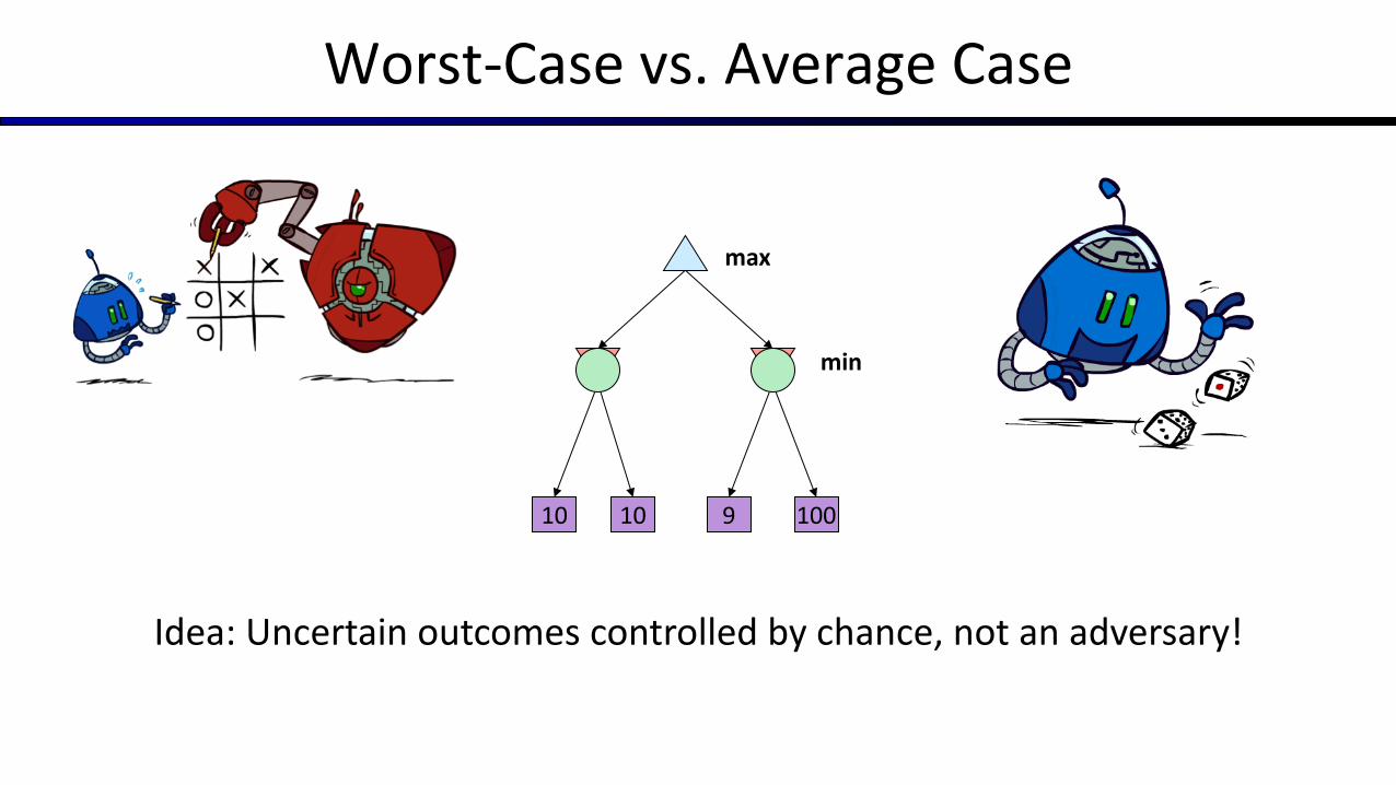
Worst-Case vs. Average Case
10 10 9 100
max
min
Idea: Uncertain outcomes controlled by chance, not an adversary!
Expectimax Search
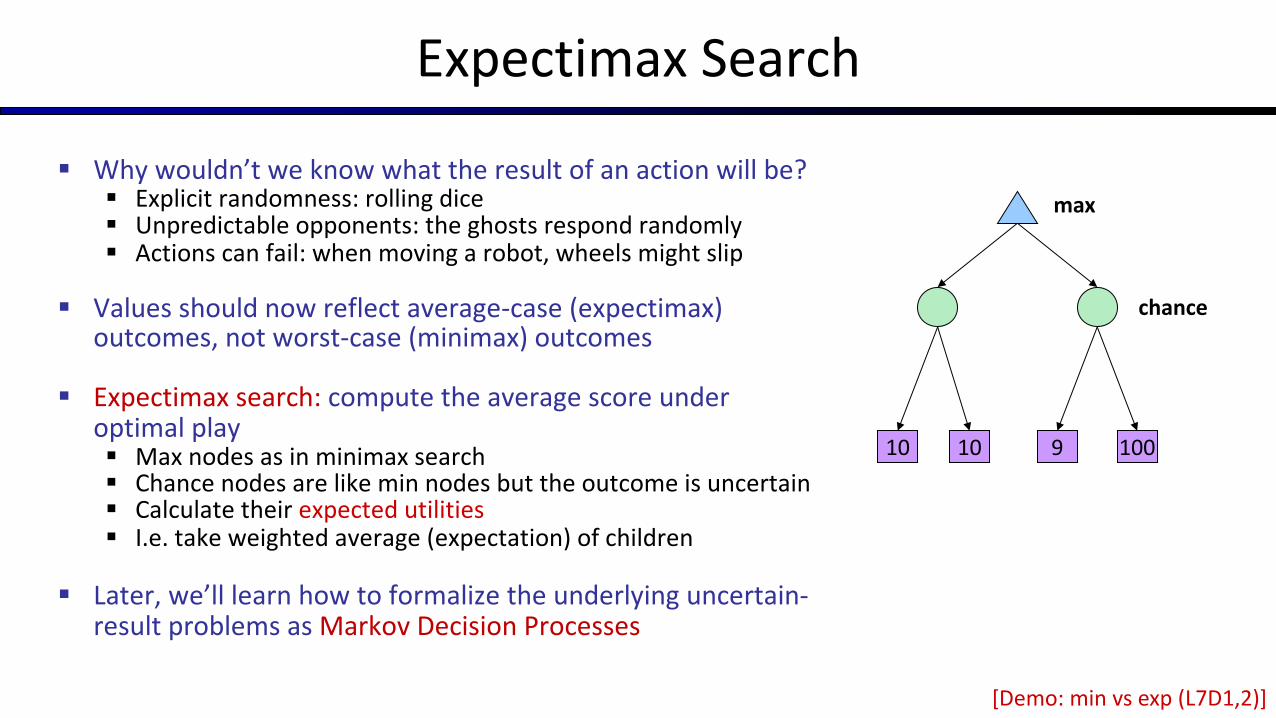
§ Why wouldn’t we know what the result of an action will be?§ Explicit randomness: rolling dice§ Unpredictable opponents: the ghosts respond randomly§ Actions can fail: when moving a robot, wheels might slip
§ Values should now reflect average-case (expectimax) outcomes, not worst-case (minimax) outcomes
§ Expectimax search: compute the average score under optimal play§ Max nodes as in minimax search§ Chance nodes are like min nodes but the outcome is uncertain§ Calculate their expected utilities§ I.e. take weighted average (expectation) of children
§ Later, we’ll learn how to formalize the underlying uncertain-result problems as Markov Decision Processes
10 4 5 7
max
chance
10 10 9 100
[Demo: min vs exp (L7D1,2)]
Video of Demo Minimax vs Expectimax (Min)

Video of Demo Minimax vs Expectimax (Exp)
Expectimax Pseudocode
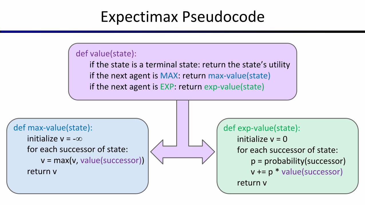
def value(state):if the state is a terminal state: return the state’s utilityif the next agent is MAX: return max-value(state)if the next agent is EXP: return exp-value(state)
def exp-value(state):initialize v = 0for each successor of state:
p = probability(successor)v += p * value(successor)
return v
def max-value(state):initialize v = -∞for each successor of state:
v = max(v, value(successor))return v
Expectimax Pseudocode
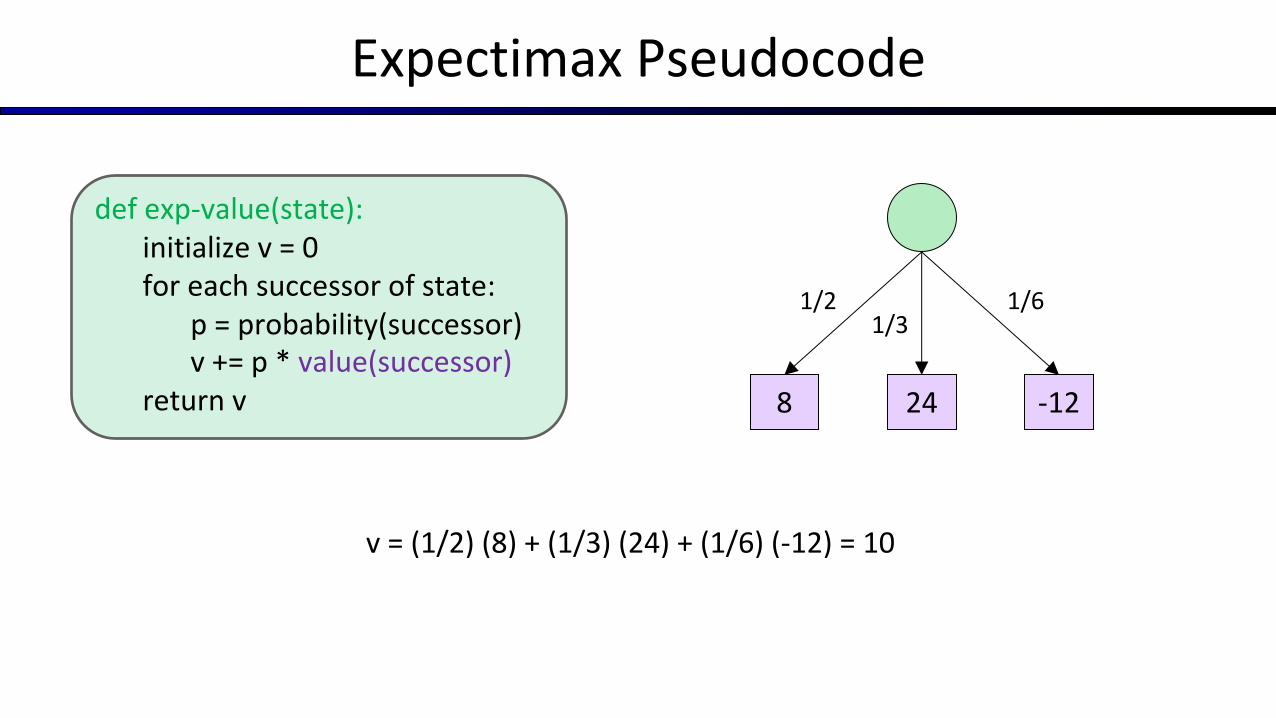
def exp-value(state):initialize v = 0for each successor of state:
p = probability(successor)v += p * value(successor)
return v 5 78 24 -12
1/21/3
1/6
v = (1/2) (8) + (1/3) (24) + (1/6) (-12) = 10
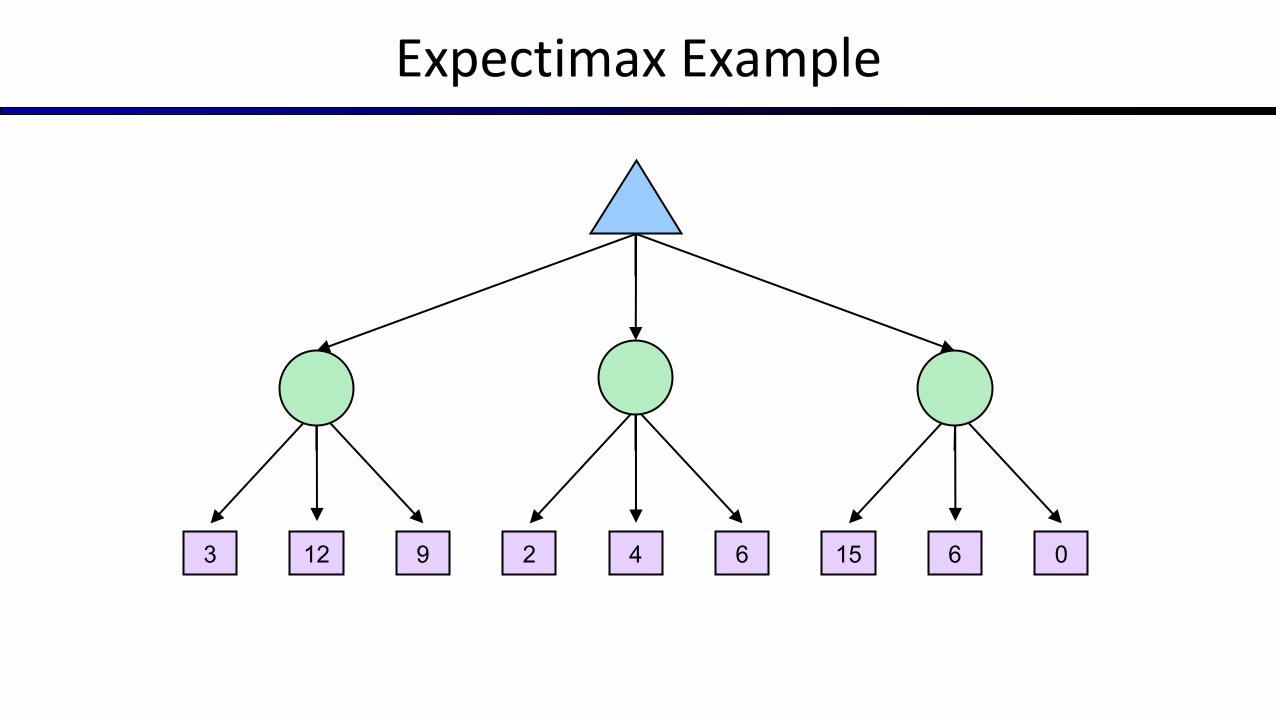
Expectimax Example
12 9 6 03 2 154 6
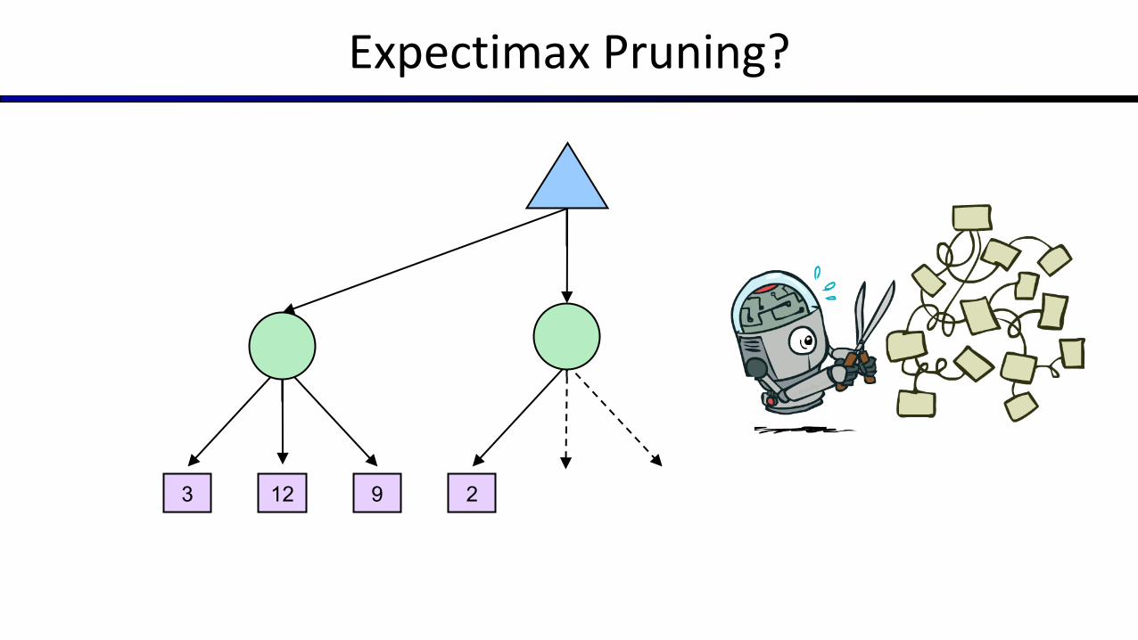
Expectimax Pruning?
12 93 2
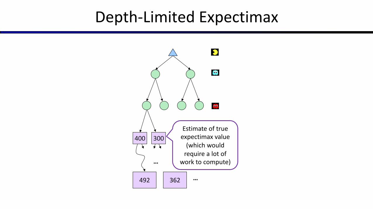
Depth-Limited Expectimax
…
…
492 362 …
400 300Estimate of true
expectimax value (which would
require a lot of work to compute)
Probabilities
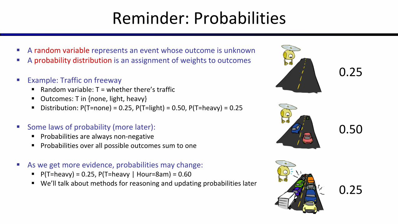
Reminder: Probabilities§ A random variable represents an event whose outcome is unknown§ A probability distribution is an assignment of weights to outcomes
§ Example: Traffic on freeway§ Random variable: T = whether there’s traffic§ Outcomes: T in {none, light, heavy}§ Distribution: P(T=none) = 0.25, P(T=light) = 0.50, P(T=heavy) = 0.25
§ Some laws of probability (more later):§ Probabilities are always non-negative§ Probabilities over all possible outcomes sum to one
§ As we get more evidence, probabilities may change:§ P(T=heavy) = 0.25, P(T=heavy | Hour=8am) = 0.60§ We’ll talk about methods for reasoning and updating probabilities later
0.25
0.50
0.25
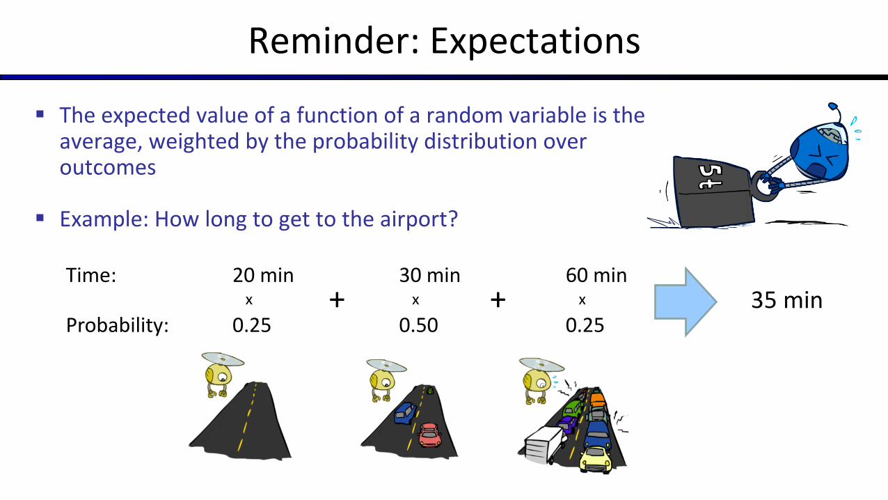
§ The expected value of a function of a random variable is the average, weighted by the probability distribution over outcomes
§ Example: How long to get to the airport?
Reminder: Expectations
0.25 0.50 0.25Probability:
20 min 30 min 60 minTime:35 minx x x+ +
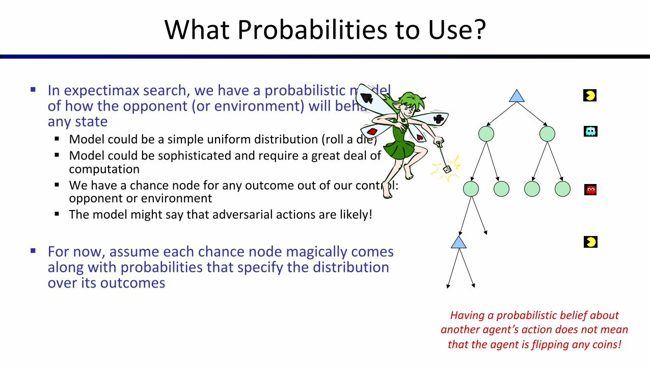
§ In expectimax search, we have a probabilistic model of how the opponent (or environment) will behave in any state§ Model could be a simple uniform distribution (roll a die)§ Model could be sophisticated and require a great deal of
computation§ We have a chance node for any outcome out of our control:
opponent or environment§ The model might say that adversarial actions are likely!
§ For now, assume each chance node magically comes along with probabilities that specify the distribution over its outcomes
What Probabilities to Use?
Having a probabilistic belief about another agent’s action does not mean
that the agent is flipping any coins!
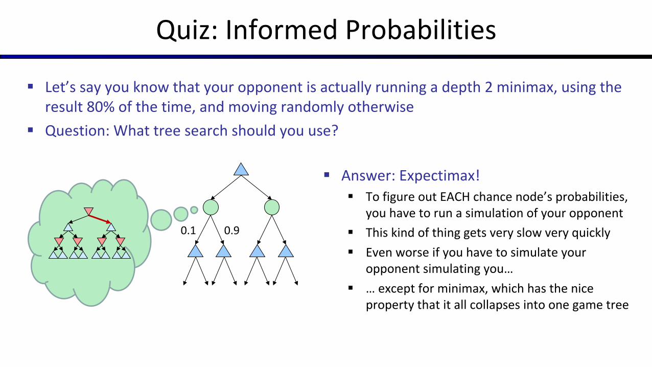
Quiz: Informed Probabilities
§ Let’s say you know that your opponent is actually running a depth 2 minimax, using the result 80% of the time, and moving randomly otherwise
§ Question: What tree search should you use?
0.1 0.9
§ Answer: Expectimax!§ To figure out EACH chance node’s probabilities,
you have to run a simulation of your opponent§ This kind of thing gets very slow very quickly§ Even worse if you have to simulate your
opponent simulating you…§ … except for minimax, which has the nice
property that it all collapses into one game tree
Modeling Assumptions
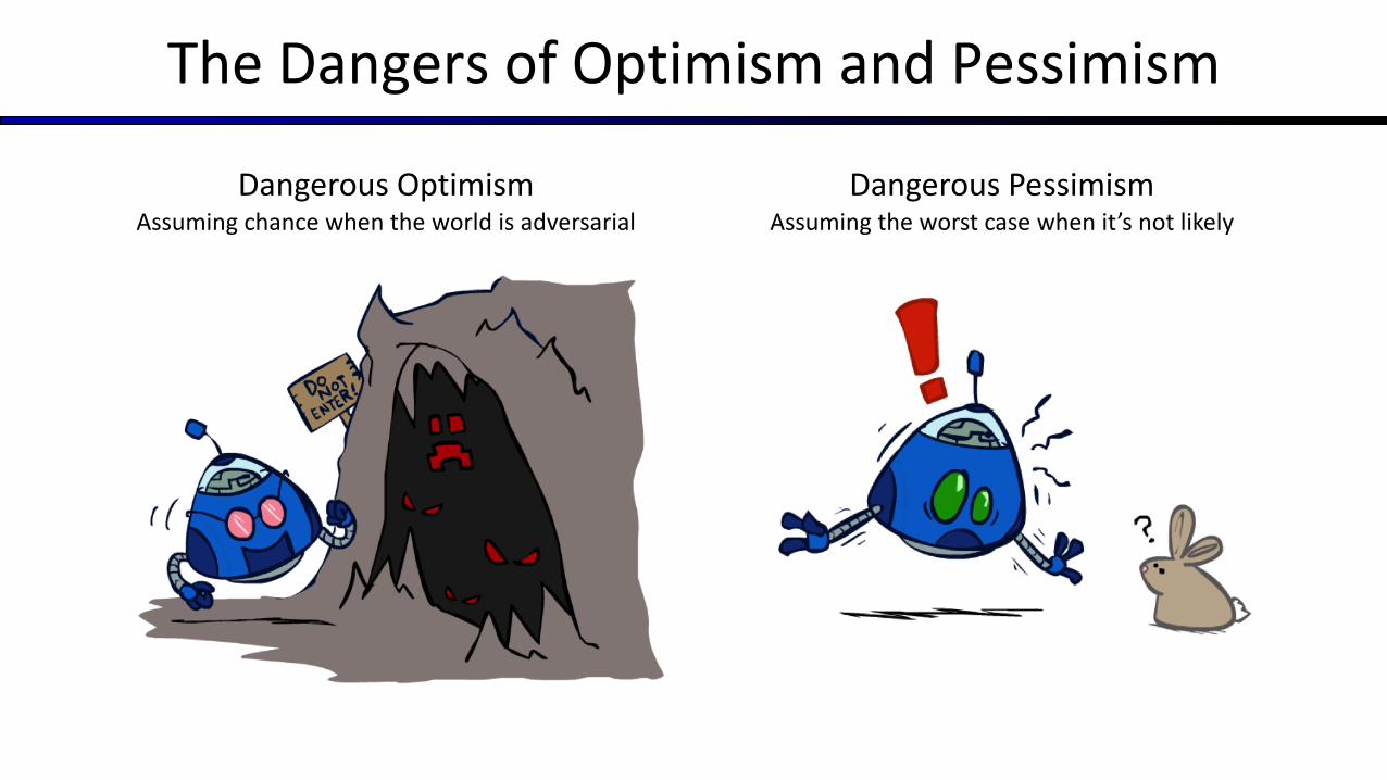
The Dangers of Optimism and Pessimism
Dangerous OptimismAssuming chance when the world is adversarial
Dangerous PessimismAssuming the worst case when it’s not likely
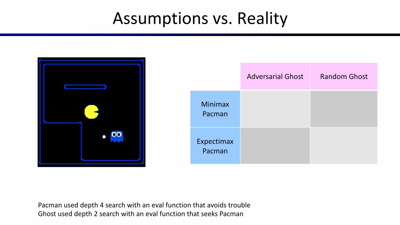
Assumptions vs. Reality
Adversarial Ghost Random Ghost
MinimaxPacman
ExpectimaxPacman
Pacman used depth 4 search with an eval function that avoids troubleGhost used depth 2 search with an eval function that seeks Pacman
Video of Demo World AssumptionsRandom Ghost – Expectimax Pacman
Video of Demo World AssumptionsAdversarial Ghost – Minimax Pacman
Video of Demo World AssumptionsAdversarial Ghost – Expectimax Pacman
Video of Demo World AssumptionsRandom Ghost – Minimax Pacman

Assumptions vs. Reality
Adversarial Ghost Random Ghost
MinimaxPacman
Won 5/5
Avg. Score: 483
Won 5/5
Avg. Score: 493
ExpectimaxPacman
Won 1/5
Avg. Score: -303
Won 5/5
Avg. Score: 503
Results from playing 5 games
Pacman used depth 4 search with an eval function that avoids troubleGhost used depth 2 search with an eval function that seeks Pacman
Other Game Types
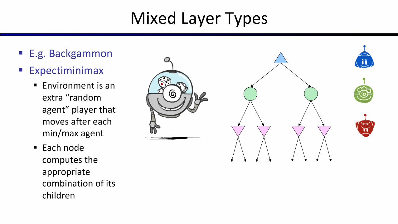
Mixed Layer Types
§ E.g. Backgammon§ Expectiminimax
§ Environment is an extra “random agent” player that moves after each min/max agent
§ Each node computes the appropriate combination of its children
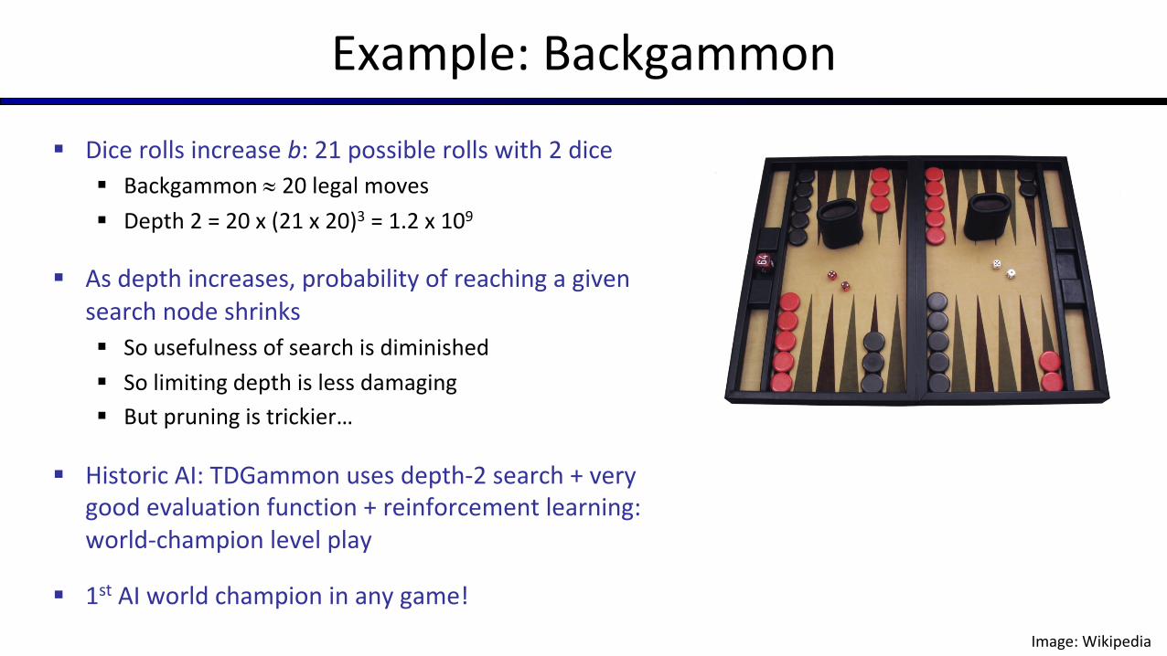
Example: Backgammon
§ Dice rolls increase b: 21 possible rolls with 2 dice§ Backgammon » 20 legal moves§ Depth 2 = 20 x (21 x 20)3 = 1.2 x 10⁹
§ As depth increases, probability of reaching a given search node shrinks§ So usefulness of search is diminished§ So limiting depth is less damaging§ But pruning is trickier…
§ Historic AI: TDGammon uses depth-2 search + very good evaluation function + reinforcement learning: world-champion level play
§ 1st AI world champion in any game!Image: Wikipedia
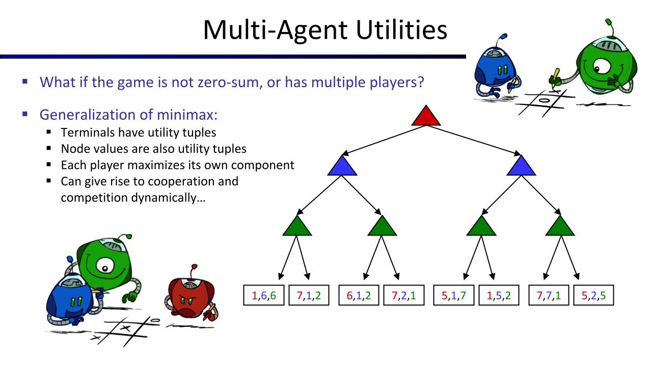
Multi-Agent Utilities
§ What if the game is not zero-sum, or has multiple players?
§ Generalization of minimax:§ Terminals have utility tuples§ Node values are also utility tuples§ Each player maximizes its own component§ Can give rise to cooperation and
competition dynamically…
1,6,6 7,1,2 6,1,2 7,2,1 5,1,7 1,5,2 7,7,1 5,2,5
Utilities
Maximum Expected Utility
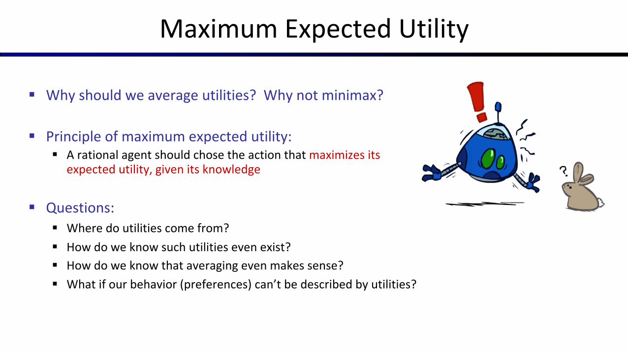
§ Why should we average utilities? Why not minimax?
§ Principle of maximum expected utility:§ A rational agent should chose the action that maximizes its
expected utility, given its knowledge
§ Questions:§ Where do utilities come from?§ How do we know such utilities even exist?§ How do we know that averaging even makes sense?§ What if our behavior (preferences) can’t be described by utilities?
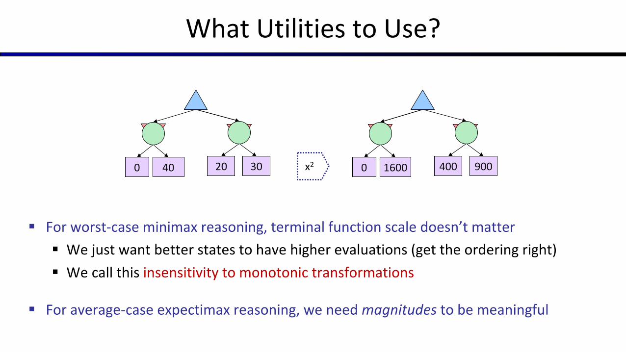
What Utilities to Use?
§ For worst-case minimax reasoning, terminal function scale doesn’t matter§ We just want better states to have higher evaluations (get the ordering right)§ We call this insensitivity to monotonic transformations
§ For average-case expectimax reasoning, we need magnitudes to be meaningful
0 40 20 30 x2 0 1600 400 900
Utilities
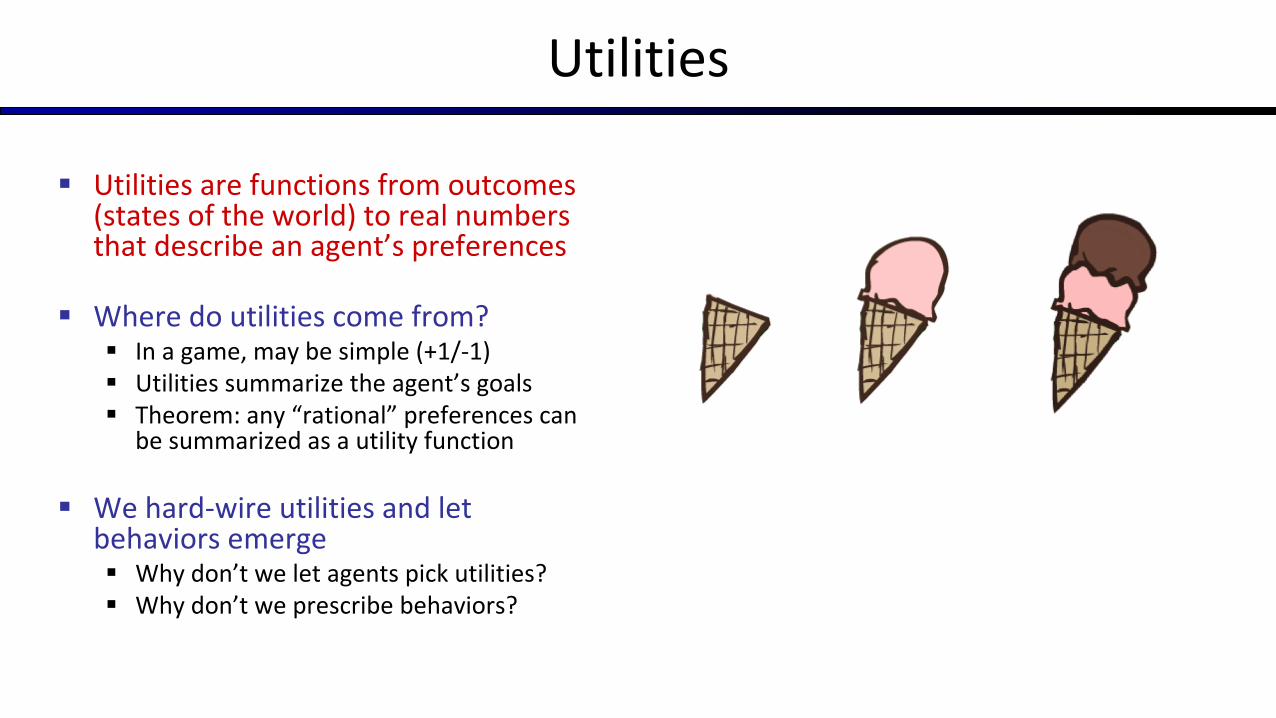
§ Utilities are functions from outcomes (states of the world) to real numbers that describe an agent’s preferences
§ Where do utilities come from?§ In a game, may be simple (+1/-1)§ Utilities summarize the agent’s goals§ Theorem: any “rational” preferences can
be summarized as a utility function
§ We hard-wire utilities and let behaviors emerge§ Why don’t we let agents pick utilities?§ Why don’t we prescribe behaviors?
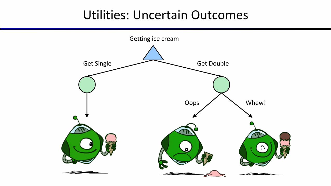
Utilities: Uncertain OutcomesGetting ice cream
Get Single Get Double
Oops Whew!
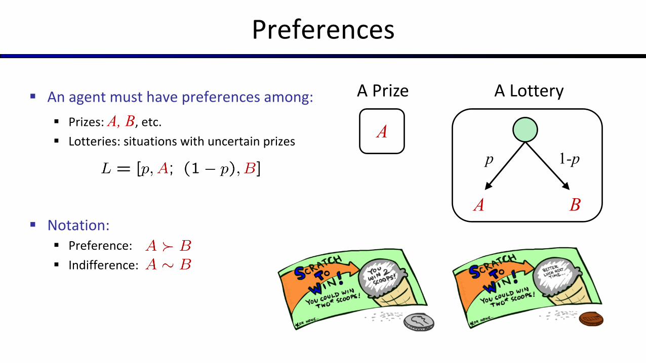
Preferences
§ An agent must have preferences among:§ Prizes: A, B, etc.§ Lotteries: situations with uncertain prizes
§ Notation:§ Preference:§ Indifference:
A B
p 1-p
A LotteryA Prize
A
Rationality
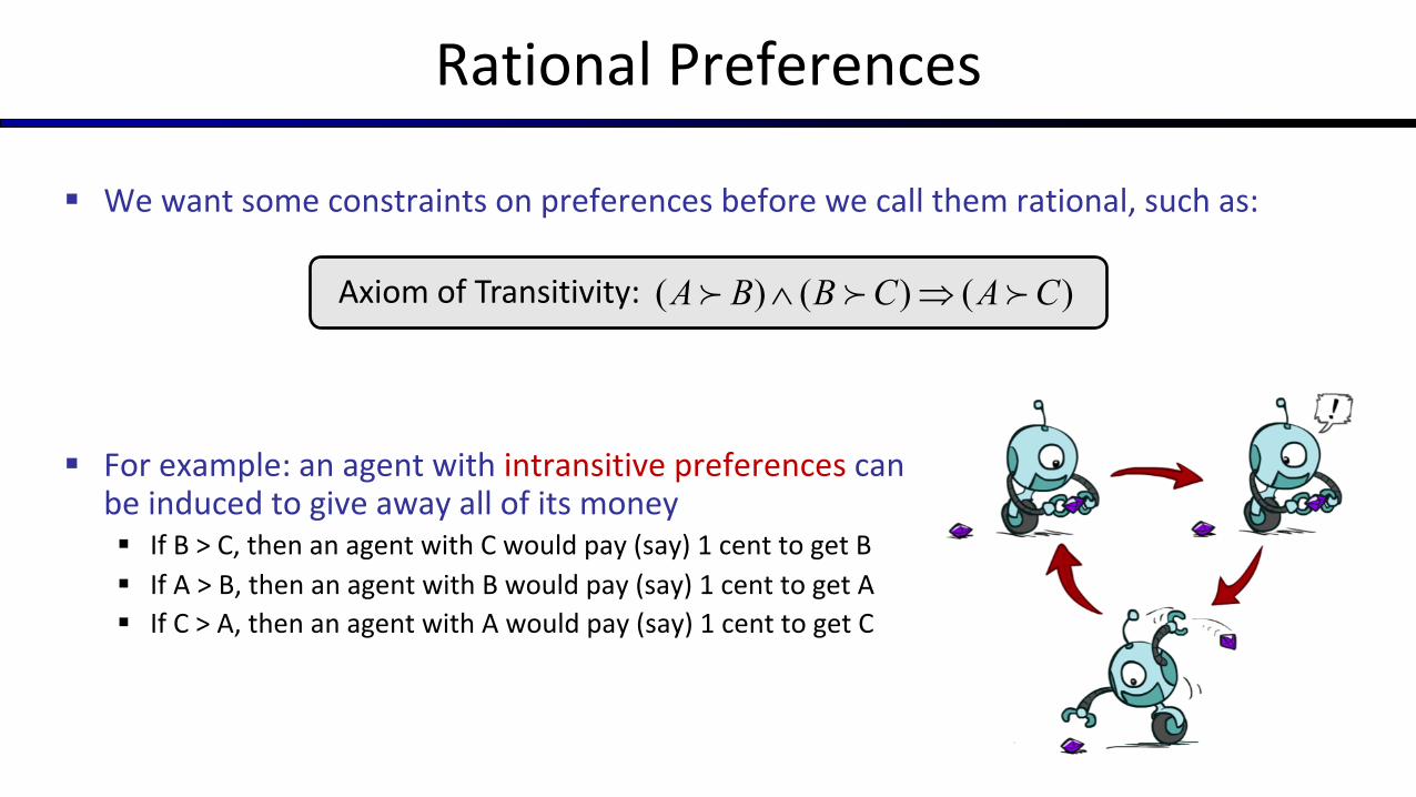
§ We want some constraints on preferences before we call them rational, such as:
§ For example: an agent with intransitive preferences canbe induced to give away all of its money§ If B > C, then an agent with C would pay (say) 1 cent to get B§ If A > B, then an agent with B would pay (say) 1 cent to get A§ If C > A, then an agent with A would pay (say) 1 cent to get C
Rational Preferences
)()()( CACBBA !!! ÞÙAxiom of Transitivity:
Rational Preferences
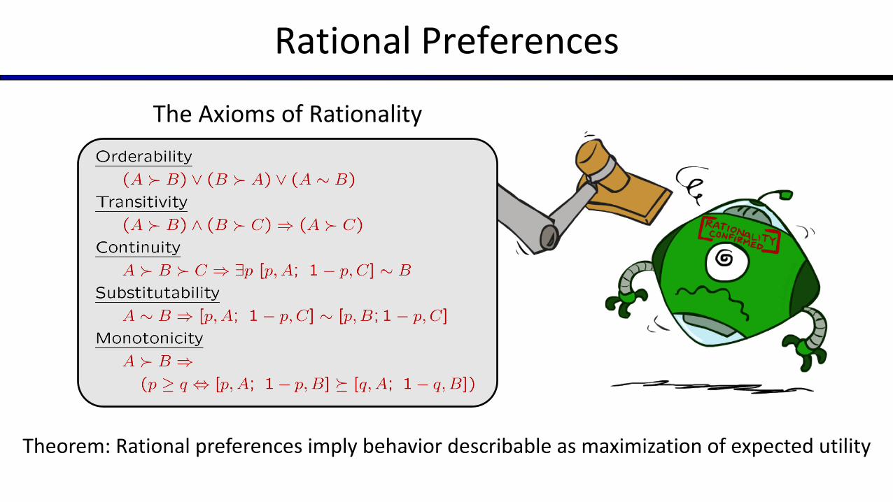
Theorem: Rational preferences imply behavior describable as maximization of expected utility
The Axioms of Rationality
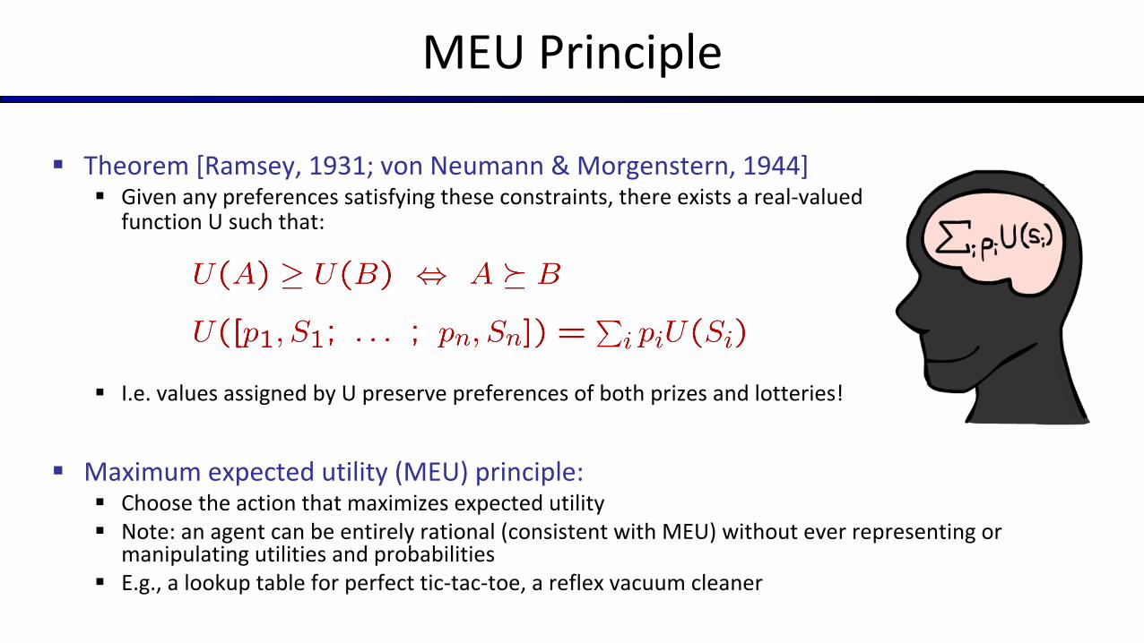
§ Theorem [Ramsey, 1931; von Neumann & Morgenstern, 1944]§ Given any preferences satisfying these constraints, there exists a real-valued
function U such that:
§ I.e. values assigned by U preserve preferences of both prizes and lotteries!
§ Maximum expected utility (MEU) principle:§ Choose the action that maximizes expected utility§ Note: an agent can be entirely rational (consistent with MEU) without ever representing or
manipulating utilities and probabilities§ E.g., a lookup table for perfect tic-tac-toe, a reflex vacuum cleaner
MEU Principle
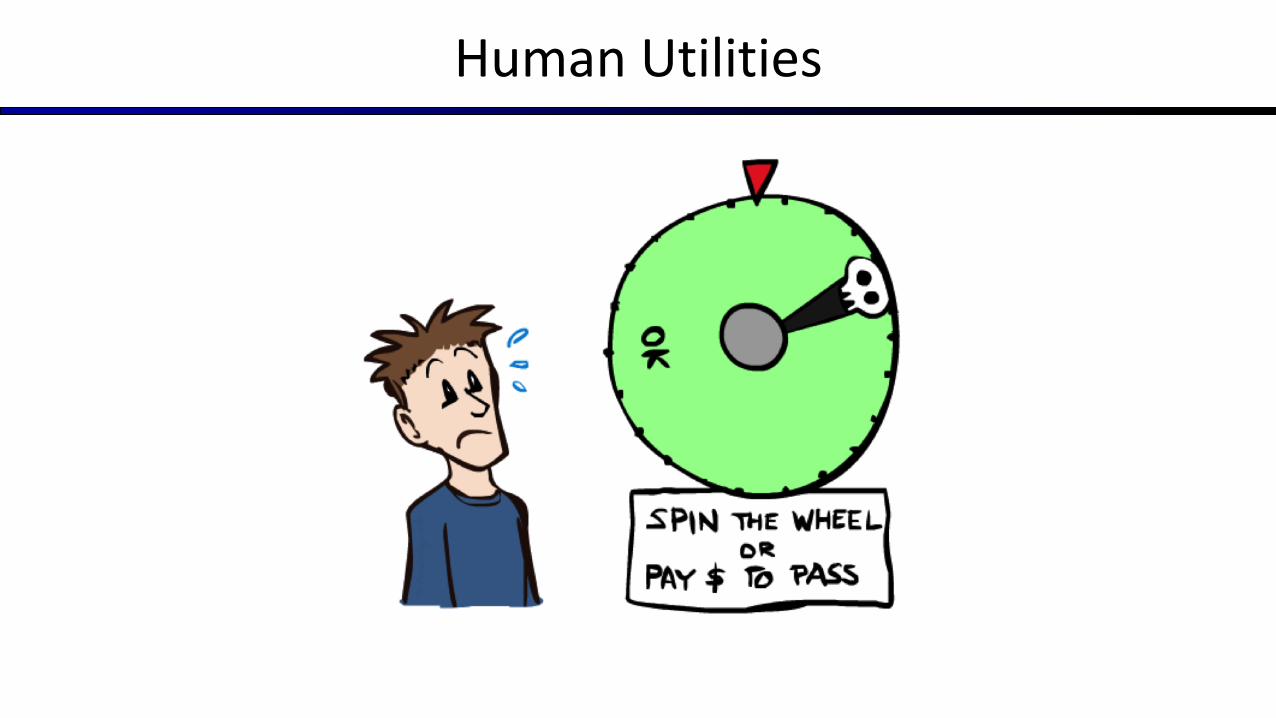
Human Utilities
Utility Scales
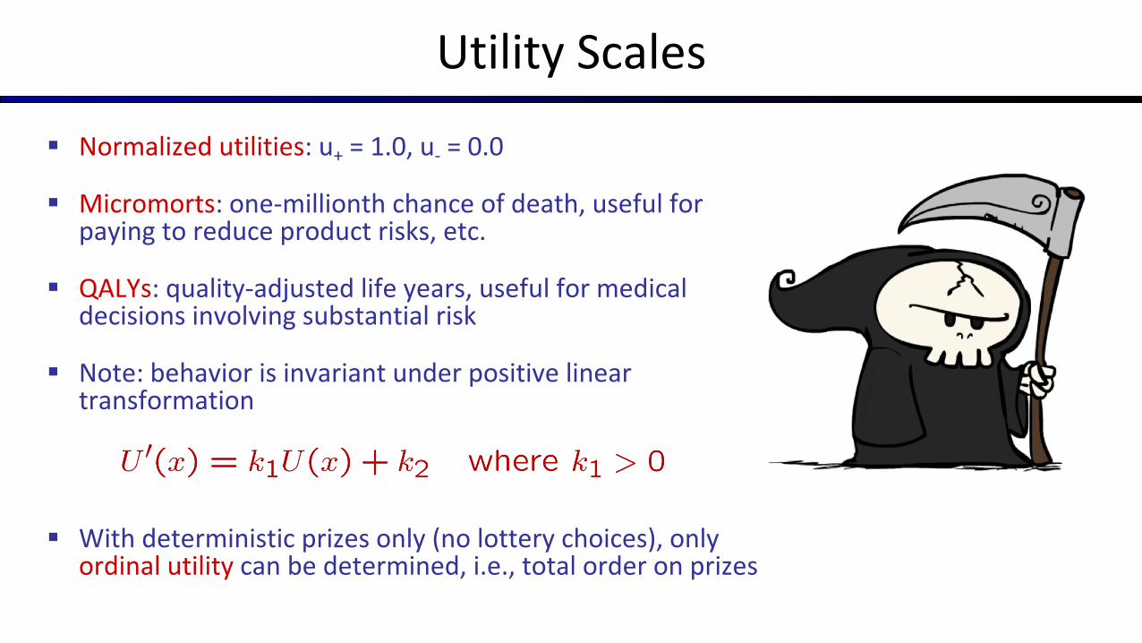
§ Normalized utilities: u+ = 1.0, u- = 0.0
§ Micromorts: one-millionth chance of death, useful for paying to reduce product risks, etc.
§ QALYs: quality-adjusted life years, useful for medical decisions involving substantial risk
§ Note: behavior is invariant under positive linear transformation
§ With deterministic prizes only (no lottery choices), only ordinal utility can be determined, i.e., total order on prizes
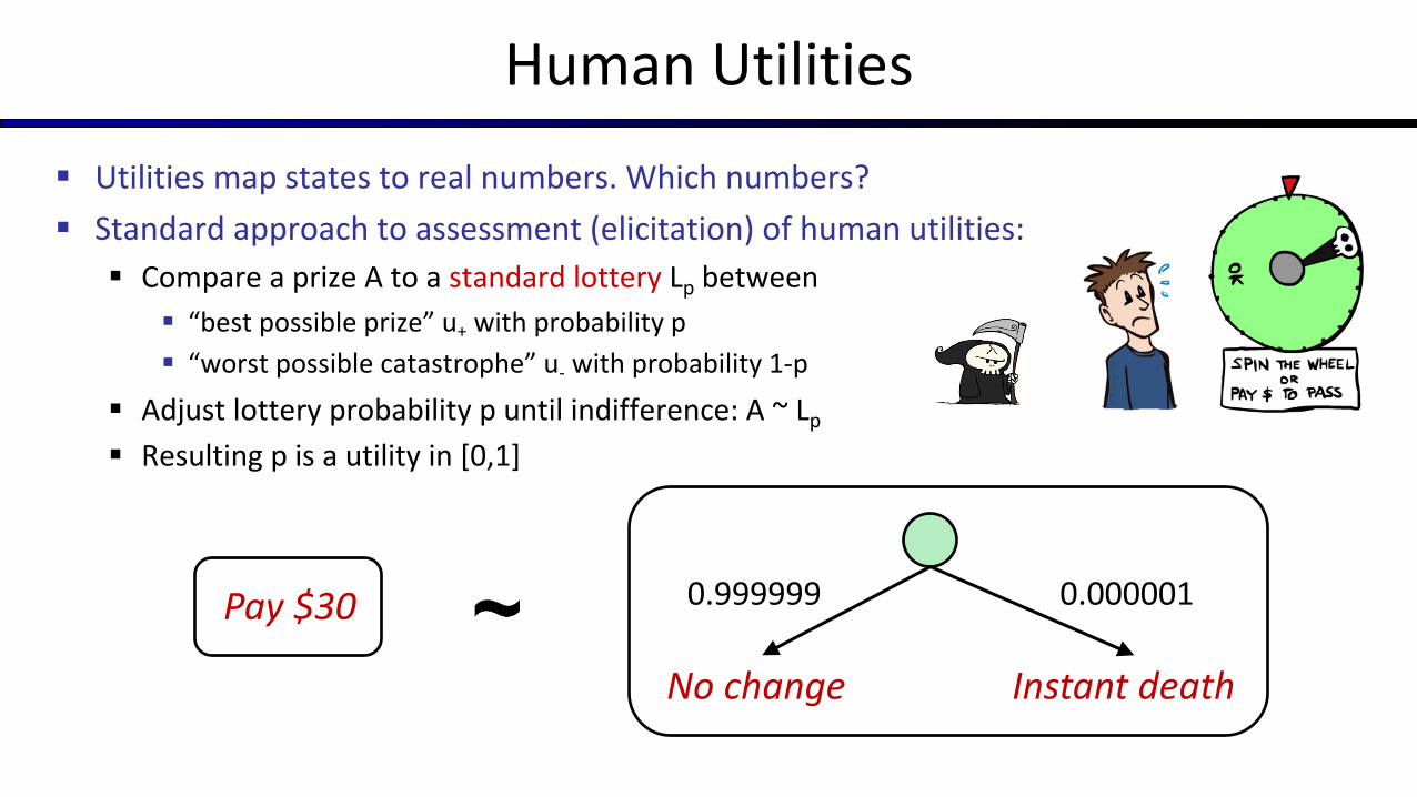
§ Utilities map states to real numbers. Which numbers?§ Standard approach to assessment (elicitation) of human utilities:
§ Compare a prize A to a standard lottery Lp between§ “best possible prize” u+ with probability p§ “worst possible catastrophe” u- with probability 1-p
§ Adjust lottery probability p until indifference: A ~ Lp
§ Resulting p is a utility in [0,1]
Human Utilities
0.999999 0.000001
No change
Pay $30
Instant death
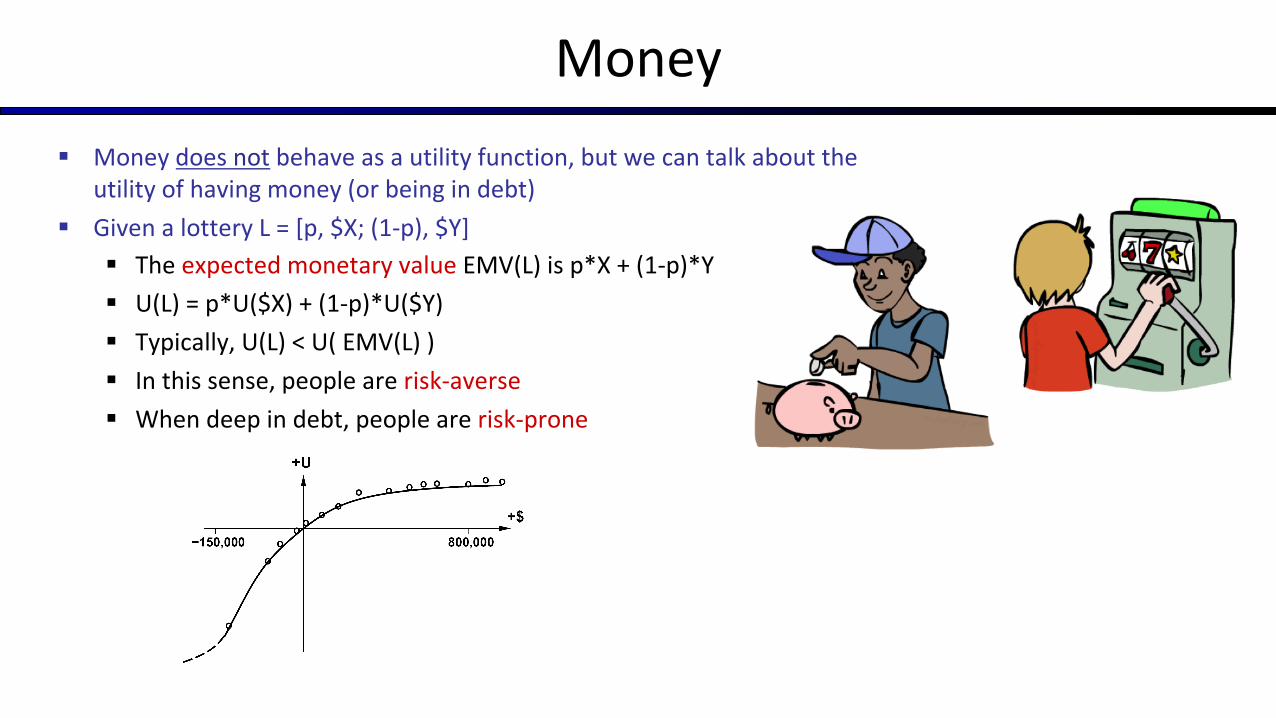
Money§ Money does not behave as a utility function, but we can talk about the
utility of having money (or being in debt)§ Given a lottery L = [p, $X; (1-p), $Y]
§ The expected monetary value EMV(L) is p*X + (1-p)*Y§ U(L) = p*U($X) + (1-p)*U($Y)§ Typically, U(L) < U( EMV(L) )§ In this sense, people are risk-averse§ When deep in debt, people are risk-prone
Example: Insurance
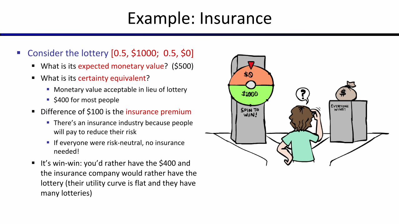
§ Consider the lottery [0.5, $1000; 0.5, $0]§ What is its expected monetary value? ($500)§ What is its certainty equivalent?
§ Monetary value acceptable in lieu of lottery§ $400 for most people
§ Difference of $100 is the insurance premium§ There’s an insurance industry because people
will pay to reduce their risk§ If everyone were risk-neutral, no insurance
needed!
§ It’s win-win: you’d rather have the $400 and the insurance company would rather have the lottery (their utility curve is flat and they have many lotteries)
Example: Human Rationality?
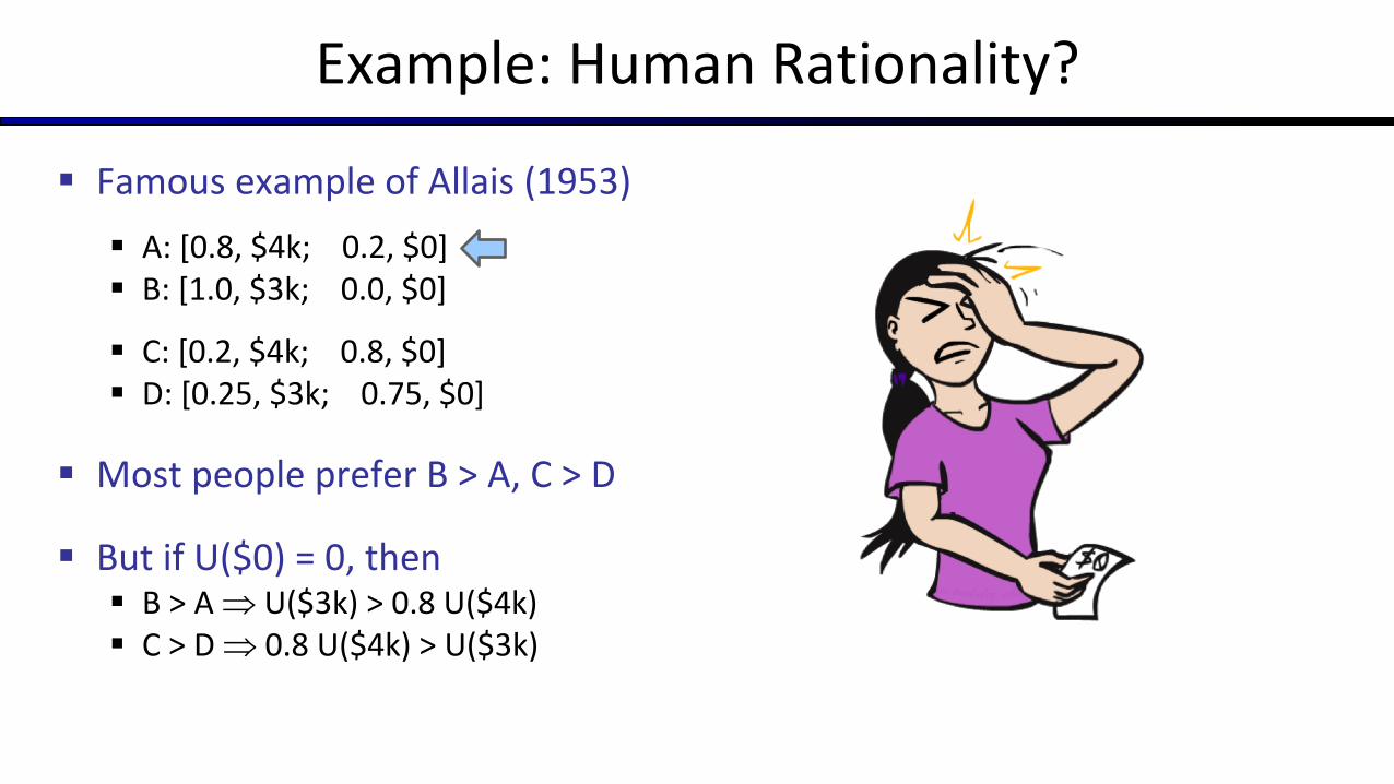
§ Famous example of Allais (1953)§ A: [0.8, $4k; 0.2, $0]§ B: [1.0, $3k; 0.0, $0]
§ C: [0.2, $4k; 0.8, $0]§ D: [0.25, $3k; 0.75, $0]
§ Most people prefer B > A, C > D
§ But if U($0) = 0, then§ B > A Þ U($3k) > 0.8 U($4k)§ C > D Þ 0.8 U($4k) > U($3k)
Next Time: MDPs!


![(Pseudo) Randomness [2ex]](https://img.pdfslide.us/doc/110x75/61570689a097e25c765040f3/pseudo-randomness-2ex.jpg)