Annals of Economics and Finance - down.aefweb.netdown.aefweb.net/AefArticles/aef150209Nilsson.pdf · IFAU – Crime, unemployment and labor market programs in turbulent times 1 Crime,

Annals of Economics and Finance

Forthcoming Article

IFAU – Crime, unemployment and labor market programs in turbulent times 1

Crime, unemployment and labor market programs in turbulent times#

by

Anna Nilsson* and Jonas Agell**

14 October 2003

Abstract We exploit the exceptional variation in municipality-level unemployment and spending on labor market programs in Sweden during the 1990s to identify the impact of unemployment and programs on crime. We identify a statistically significant effect of unemployment on the incidence of overall crime, burglary, auto-theft and drug possession. A calculation suggests that the sharp reduction in unemployment during the later 1990s may have reduced burglary and auto-theft with 15 and 20 percent, respectively. After addressing several specifi-cation issues, we conclude that there is at best weak evidence that labor market programs – general ones and those specifically targeted to the young – help to reduce crime. Jel-codes: J00, K40 Keywords: Crime, unemployment, labor market programs, panel data

# We have benefited from helpful comments from Per-Anders Edin, Peter Fredriksson, Per Johansson, Oskar Nordström Skans, Henry Ohlsson, Mårten Palme, Per Pettersson Lidbom and Peter Skogman Thoursie, as well as from seminar participants at FIEF, IFAU, Stockholm University and SOFI. We have also presented the paper at the annual meetings of EALE and EEA, and at the International microeconometrics conference, Dublin, 22-23 May. This research was funded by a grant from IFAU (Institute for Labour Market Policy Evaluation). * Stockholm University; address: Department of Economics, Stockholm University, SE-106 91 Stockholm; email: [email protected] ** Stockholm University and CESifo; address: Department of Economics, Stockholm University, SE-106 91 Stockholm; email: [email protected]

IFAU – Crime, unemployment and labor market programs in turbulent times

2

Table of contents

1 Introduction ............................................................................................... 3

2 Data and empirical specification ............................................................... 6

3 Our baseline specification ....................................................................... 12

4 Alternative specifications ........................................................................ 14

5 Youthful crimes and youth unemployment ............................................. 19

6 Conclusions ............................................................................................. 26

References.......................................................................................................... 27

Appendix 1: Definitions of variables ................................................................. 29

Appendix 2: Results for the baseline specification............................................ 30

Appendix 3: Instruments for municipality-level unemployment ....................... 31


1 Introduction Does unemployment and poor labor market opportunities lead to increased crime? This paper uses a new panel data set for Swedish municipalities for the period 1996–2000 to explore how unemployment affects crime. During this period the overall unemployment rate (including those enrolled in labor market programs) decreased from 11.9 to 6.8 percent, and for those most likely to commit crimes, people under the age of 25, unemployment decreased from 21.2 to 8.7 percent. But the decrease in unemployment was far from uniform across the country, and our identification strategy is to use the large variation in the improvement in labor market conditions across municipalities to isolate the relationship between unemployment and crime.

Many models of crime suggest that the unemployed, and individuals with low wages, face strong incentives to commit (property) crimes. Following Becker (1968), the economics of crime pictures an amoral individual, who bases his choice of whether to become a criminal on a comparison of the returns to legal and illegal activities. Since involuntary unemployment can be expected to reduce the return to working in the legal sector, there will be a substitution effect that induces people to commit more crime.1 The idea that unemployment breeds crime also has a long tradition in e.g. sociology and criminology. It is a common view that crime is the outcome of social inter-actions, and that unemployment creates a criminal culture within certain segments of society.

The empirical evidence on the link between unemployment and crime is not clear-cut; for reviews, see Chiricos (1987) on the older literature, and Freeman (1999) on the more recent one. Though some studies indicate that crime has a positive association with unemployment, there are many studies suggesting that the relationship is weak or nonexistent.2 However, upon addressing a number of econometric complications two recent panel studies report magnitudes that appear to be statistically and economically significant. Using U.S. state-level data Raphael and Winter-Ebmer (2001) report results indicating that a sub- 1 See e.g. Freeman (1999). There are extended economic models of crime where the link between unemployment and criminal activity is less clear-cut. In a model where people can commit crime while working, unemployment may have a zero impact, see e.g. Grogger (1998). 2 Less than 50 percent of the studies surveyed by Chiricos (1987) find positive, significant effects of aggregate unemployment on crime. But Chiricos also notes that the relationship between unemployment and property crime is frequently positive and significant.


4

stantial portion of the decline in U.S. property crime rates during the 1990s is attributable to the decline in the unemployment rate. Using U.S. county-level data Gould, Weinberg and Mustard (2002) show that the unemployment rate of non-college educated men is significantly correlated with property crimes like auto-theft and burglary.

We believe that our paper is a useful contribution for the following reasons. First, the huge variation in Swedish unemployment during the 1990s provides an ideal opportunity to isolate the effect of unemployment on crime. Most studies exploit data for countries and periods in which unemployment is fairly stable, or changes steadily over time. With such data it is not easy to separate the effect of unemployment from the effect of general time trends, and to avoid that omitted variables bias the result. In our data, variations in unemployment dwarf the fluctuations in other covariates, which mitigates these problems. Moreover, since the variation in Swedish unemployment can be traced to macroeconomic3 events, which are exogenous to the municipality, bias due to reverse causation in the crime-unemployment dimension should be a lesser problem.

Second, since we have detailed information about economic and demo-graphic developments in 288 out of Sweden’s 289 municipalities,4 we can further reduce the risk of omitted variable bias. For example, since unem-ployment is higher for workers with low wages, and for individuals with little schooling, a regression that fails to control for schooling/unskilled wages may easily bias the estimate of the effect of unemployment on crime. Below, we include municipality-level measures of educational composition among our regressors. Third, since young individuals are responsible for a dispropor-tionate share of many crimes the unemployment rate for this group ought to be of particular importance for students of crime and unemployment. Yet, recent studies have focused on unemployment rates for much broader groups. By contrast we have annual data on the number of unemployed, both in the aggregate population of working-age, as well as for different subgroups, including those aged 18–24.

Fourth, a large literature explores how labor market programs affect sub-sequent earnings; see e.g. Calmfors, Forslund and Hemström (2002). We focus on a different effect: does placement in labor market programs reduce crime?

3 For a discussion of the Swedish macroeconomic crisis of the 1990s, see Lindbeck (1997). 4 In our regressions we exclude one of them, Nykvarn, which was formed only in 1999.


Such an effect could arise for many reasons. Program participation may imply: (i) that there is less time for other activities, including crime; (ii) social interactions that prevent the participant from adopting the wrong kind of social norms; (iii) a greater ability to earn legal income in the labor market. To the best of our knowledge no other study has explored this issue.

Finally, in view of the social and economic issues at stake, it is surprising that there is so little evidence on these issues for countries other than the USA. Of the 63 studies reviewed by Chiricos (1987) no less than 52 rely on US data, and there is no mentioning of studies for other European countries than the UK. We believe that the Swedish experience is interesting in its own right, and that it is a worthwhile exercise to analyze whether the relationship between unem-ployment and crime is of a different nature in a welfare state, with generous social transfers.5

Our results indicate that there is a statistically significant correlation between the overall unemployment rate and the incidence of overall crime, burglary, auto-theft and drug possession. A calculation suggests that the sharp reduction in unemployment during the late 1990s may have reduced burglary and auto-theft with 15 and 20 percent, respectively. These effects appear to be of such magnitudes so as to warrant the interest of policy-makers. We find much weaker evidence that labor market programs reduce crime, and there is no evidence that youth unemployment, and labor market programs targeted to the young, have an impact on criminal activity.

The next section describes our data, and presents our empirical method-ology. Section 3 reports our basic fixed effect regressions on how unemploy-ment and labor market programs affect main crime categories. Section 4 addresses specification issues, and section 5 turns to the impact of youth unemployment and youth labor market programs. A final section sums up, and suggests extensions for future research.

5 We are aware of three previous Swedish studies that analyze the link between unemployment and crime: le Grand (1986), Schuller (1986) and Edmark (2002). Le Grand uses aggregate time series data and finds a negative partial correlation between burglary and the vacancy rate. Schuller uses cross-sectional data for Swedish municipalities, and finds no significant corr-elations between crime and unemployment. Edmark (2002) finds that county unemployment is significantly correlated with property crime.


6

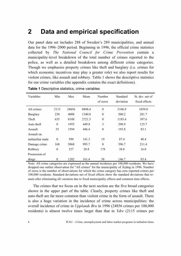
2 Data and empirical specification Our panel data set includes 288 of Sweden’s 289 municipalities, and annual data for the 1996–2000 period. Beginning in 1996, the official crime statistics collected by The National Council for Crime Prevention contain a municipality-level breakdown of the total number of crimes reported to the police, as well as a detailed breakdown among different crime categories. Though we emphasize property crimes like theft and burglary (i.e. crimes for which economic incentives may play a greater role) we also report results for violent crimes, like assault and robbery. Table 1 shows the descriptive statistics for our crime variables (the appendix contains the exact definitions). Table 1 Descriptive statistics, crime variables

Variables Min Max Mean Number of zeros

Standard deviation

St. dev. net of fixed effects

All crimes 2115 24856 8898.4 0 3106.9 1059.8 Burglary 238 4008 1340.0 0 500.2 281.7 Theft 635 8108 2721.5 0 1185.4 397.6 Auto theft 0 1955 449.8 3 298.9 125.7 Assault 35 1594 446.4 0 193.8 83.1 Assault on unfamiliar male 0 599 141.3 19 87.4 40.4 Damage crime 168 5068 995.7 0 396.7 211.4 Robbery 0 327 28.8 178 38.8 16.0 Possession of drugs 0 1202 161.4 58 146.7 93.4 Note: All crime categories are expressed as the annual incidence per 100,000 residents. We have dropped one outlier observation for "All crimes" for the municipality of Årjäng in 1996. Number of zeros is the number of observations for which the crime category has zero reported crimes per 100,000 residents. Standard deviations net of fixed effects show the standard deviations that re-main after eliminating all variation due to fixed municipality effects and common time effects.

The crimes that we focus on in the next section are the five broad categories shown in the upper part of the table. Clearly, property crimes like theft and auto-theft are far more common than violent crime in the form of assault. There is also a huge variation in the incidence of crime across municipalities: the overall incidence of crime in Upplands Bro in 1996 (24856 crimes per 100,000 residents) is almost twelve times larger than that in Ydre (2115 crimes per


100,000 residents). The lower part shows four crime categories, for which young offenders are known to be heavily over-represented, assault against unfamiliar man, damage crime, robbery and possession of drugs. The final column shows the standard deviation that remains after netting out all variation due to fixed municipality and time effects. Below, we will analyze whether this residual variation can be linked to the residual variation of local unemploy-ment.

Poor data quality is an important problem for students of crime. The crimes that are recorded by the police can be expected to underestimate true criminal activity by a relatively large margin. If this under-coverage varies system-atically over time there is cause for concern. For example, there is evidence that under-coverage has decreased for certain crime categories during the second half of the 1990s.6 Since unemployment decreased substantially during the same period there is a risk that there will be a downward bias in the crime-unemployment effect computed from the official crime statistics. Still, our empirical approach mitigates this problem to a great extent. First, for auto theft and burglary (i.e. two of the crimes that we focus on in the next section) the extent of underreporting is most probably small and stable over time.7 Second, our fixed effect specification eliminates the influence of measurement errors that (a) varies across municipalities but remain constant over time, and (b) changes in the same manner over time in all municipalities. Hence, our results will not be biased by changes in under-coverage that are common to all municipalities. Trends in under-coverage that are specific to the municipality may still bias our crime-unemployment effects, but only in so far as they are correlated with municipality-level trends in unemployment.8

The starting point for our investigation is the following model:

6 This evidence largely relies on comparisons between the official crime statistics and victimization data from household crime surveys. National Council for Crime Prevention (2001) includes detailed discussions of the development of under-coverage for main crime categories. Domestic violence against children and sexual harassment are examples of crime where under-coverage appears to have decreased. A crime category for which under-coverage increased during the second half of the 1990s is drunk driving. During this period the police shifted to less systematic monitoring practices. 7 See e.g. National Council for Crime Prevention (2001). The victims from auto theft and burglary have to report the crime to the police if they are to receive compensation from insurance companies. 8 We are however not aware of any evidence suggesting that municipality-level trends dominate the national trends in under-coverage in Swedish crime data.


8

Crimeit = αi + λt + θUnemploymentit + γProgramit + βXit + εit. (1)

Here, i and t are indices for municipality and time, Crimeit is the log of the number of crimes of a particular category per 100,000 residents, Xit is a vector of demographic and economic controls, iα is a municipality fixed effect and tλ is a year fixed effect. These fixed effects eliminate all variation in crime rates caused by factors varying across municipalities but constant over time, and vice versa. Finally, Unemploymentit and Programit are our measures of unemploy-ment and placement in labor market programs discussed below. Since the time dummies in our benchmark specification removes all national trends, we identify the impact of unemployment and program participation on crime via the within-municipality deviations from the aggregate trends. Our standard errors are robust to heteroscedasticity and consistent with respect to serial correlation within the municipality.9

Table 2 presents the descriptive statistics for our explanatory variables. For each municipality The National Labor Market Board provided us with (annual) information about the number of unemployed and the number of individuals enrolled in labor market programs, in the aggregate and for different demo-graphic groups. Statistics Sweden provided us with complete municipality-level age distributions. We constructed our unemployment rates by adding the number of unemployed and the number of individuals in programs, and dividing the total by the size of the relevant demographic group.10 To construct a measure of the incidence of programs we divided the number of individuals in programs with the sum of individuals classified as being unemployed or in programs. There is clearly considerable variation across municipalities in 9 We estimate (1) using the AREG command in Stata, and invoke the cluster-routine, treating each municipality as an independent cluster. The Monte Carlo analysis of Kézdi (2002) shows that the finite-sample bias of the robust estimators is smaller than the bias of the estimators that assume no serial correlation at any sample size. These simulations also reveal that the cluster estimator is unbiased in samples of usual size, and slightly biased downward if the cross-sectional sample is very small. In all, Table 3 below reports ten estimated semi-elasticities linking unemployment and various crimes; with our cluster-estimator, only three of these are statistically significant at the five-percent level. With the standard fixed effect estimator all standard errors are some 30 percent smaller; as a consequence two semi-elasticities would be significant at the one percent-level, and three more at the five-percent level. 10 Unemployment rates are normally computed by dividing unemployment with the labor force rather than total population. However, there is no municipality-level data on labor force participation.


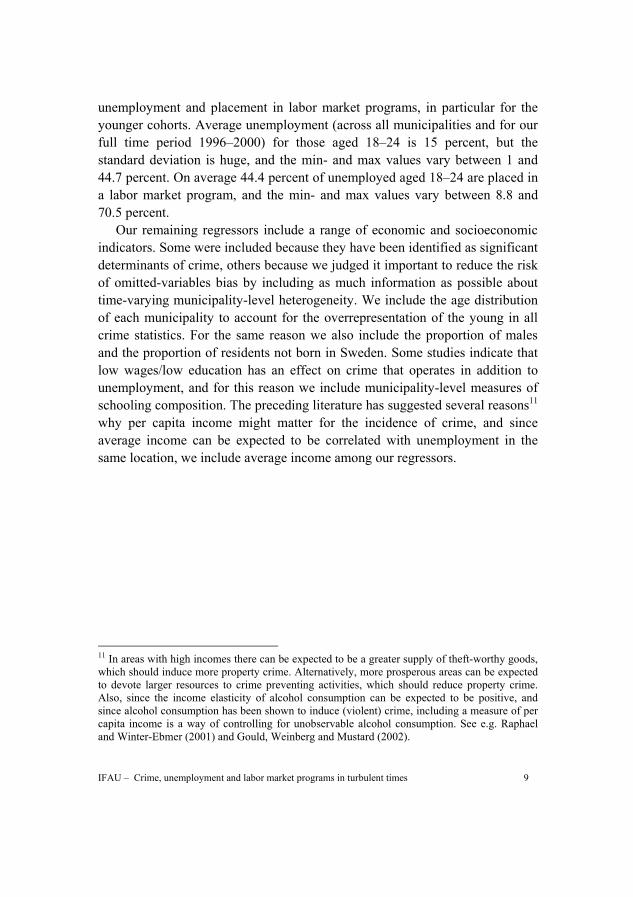
unemployment and placement in labor market programs, in particular for the younger cohorts. Average unemployment (across all municipalities and for our full time period 1996–2000) for those aged 18–24 is 15 percent, but the standard deviation is huge, and the min- and max values vary between 1 and 44.7 percent. On average 44.4 percent of unemployed aged 18–24 are placed in a labor market program, and the min- and max values vary between 8.8 and 70.5 percent.

Our remaining regressors include a range of economic and socioeconomic indicators. Some were included because they have been identified as significant determinants of crime, others because we judged it important to reduce the risk of omitted-variables bias by including as much information as possible about time-varying municipality-level heterogeneity. We include the age distribution of each municipality to account for the overrepresentation of the young in all crime statistics. For the same reason we also include the proportion of males and the proportion of residents not born in Sweden. Some studies indicate that low wages/low education has an effect on crime that operates in addition to unemployment, and for this reason we include municipality-level measures of schooling composition. The preceding literature has suggested several reasons11 why per capita income might matter for the incidence of crime, and since average income can be expected to be correlated with unemployment in the same location, we include average income among our regressors.

11 In areas with high incomes there can be expected to be a greater supply of theft-worthy goods, which should induce more property crime. Alternatively, more prosperous areas can be expected to devote larger resources to crime preventing activities, which should reduce property crime. Also, since the income elasticity of alcohol consumption can be expected to be positive, and since alcohol consumption has been shown to induce (violent) crime, including a measure of per capita income is a way of controlling for unobservable alcohol consumption. See e.g. Raphael and Winter-Ebmer (2001) and Gould, Weinberg and Mustard (2002).


10

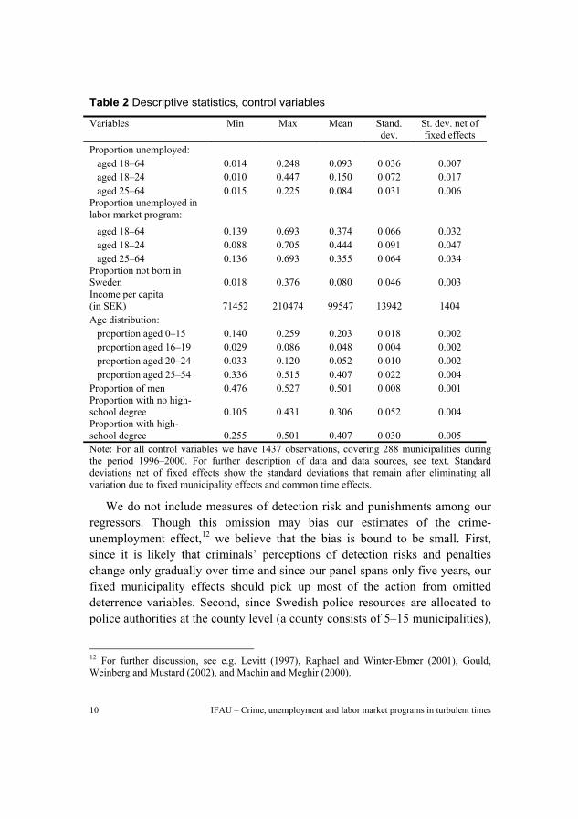
Table 2 Descriptive statistics, control variables

Variables Min Max Mean Stand. dev.

St. dev. net of fixed effects

Proportion unemployed: aged 18–64 0.014 0.248 0.093 0.036 0.007 aged 18–24 0.010 0.447 0.150 0.072 0.017 aged 25–64 0.015 0.225 0.084 0.031 0.006 Proportion unemployed in labor market program:

aged 18–64 0.139 0.693 0.374 0.066 0.032 aged 18–24 0.088 0.705 0.444 0.091 0.047 aged 25–64 0.136 0.693 0.355 0.064 0.034 Proportion not born in Sweden 0.018 0.376 0.080 0.046 0.003 Income per capita (in SEK) 71452 210474 99547 13942 1404 Age distribution: proportion aged 0–15 0.140 0.259 0.203 0.018 0.002 proportion aged 16–19 0.029 0.086 0.048 0.004 0.002 proportion aged 20–24 0.033 0.120 0.052 0.010 0.002 proportion aged 25–54 0.336 0.515 0.407 0.022 0.004 Proportion of men 0.476 0.527 0.501 0.008 0.001 Proportion with no high-school degree 0.105 0.431 0.306 0.052 0.004 Proportion with high-school degree 0.255 0.501 0.407 0.030 0.005 Note: For all control variables we have 1437 observations, covering 288 municipalities during the period 1996–2000. For further description of data and data sources, see text. Standard deviations net of fixed effects show the standard deviations that remain after eliminating all variation due to fixed municipality effects and common time effects.

We do not include measures of detection risk and punishments among our regressors. Though this omission may bias our estimates of the crime-unemployment effect,12 we believe that the bias is bound to be small. First, since it is likely that criminals’ perceptions of detection risks and penalties change only gradually over time and since our panel spans only five years, our fixed municipality effects should pick up most of the action from omitted deterrence variables. Second, since Swedish police resources are allocated to police authorities at the county level (a county consists of 5–15 municipalities),

12 For further discussion, see e.g. Levitt (1997), Raphael and Winter-Ebmer (2001), Gould, Weinberg and Mustard (2002), and Machin and Meghir (2000).


most of the differences in police resources between municipalities ought to follow county rather than municipality borders. To check this, we added county dummies to all our regressions; it turned out that these were typically stat-istically insignificant, and of no consequence for the coefficients of primary interest. Third, our yearly time dummies eliminate the contaminating influence from changes in deterrence variables that are common to all municipalities. Finally, in section 4 we use an instrumental variables technique that (among other things) deals with the potential bias from omitted variables.

A comparison of the two final columns of Table 2 shows that most of our regressors have little independent variation, once we eliminate all variation due to general time trends and municipality fixed effects. For our age, gender and schooling variables the residual standard deviations fall in the interval .001–.004. For our variables of primary interest, unemployment and placement in programs for different age groups, the residual standard deviations are typically about ten times as high. Compared to previous panel studies of the relationship between crime and unemployment we have unusually large independent var-iation in our labor market variables. For example, Raphael and Winter-Ebmer (2001, table 1) report that the residual variation of their unemployment variable is of the same order of magnitude as the residual variation for their other main regressors (black, poor and age structure). Since the standard error of the coefficient of a given independent variable decreases with the total sample variation of the same variable this suggests that we can obtain comparatively precise estimates of the coefficients on our unemployment and program variables.

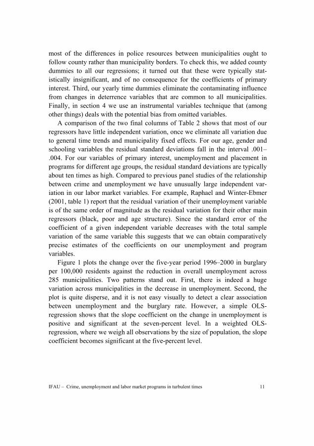
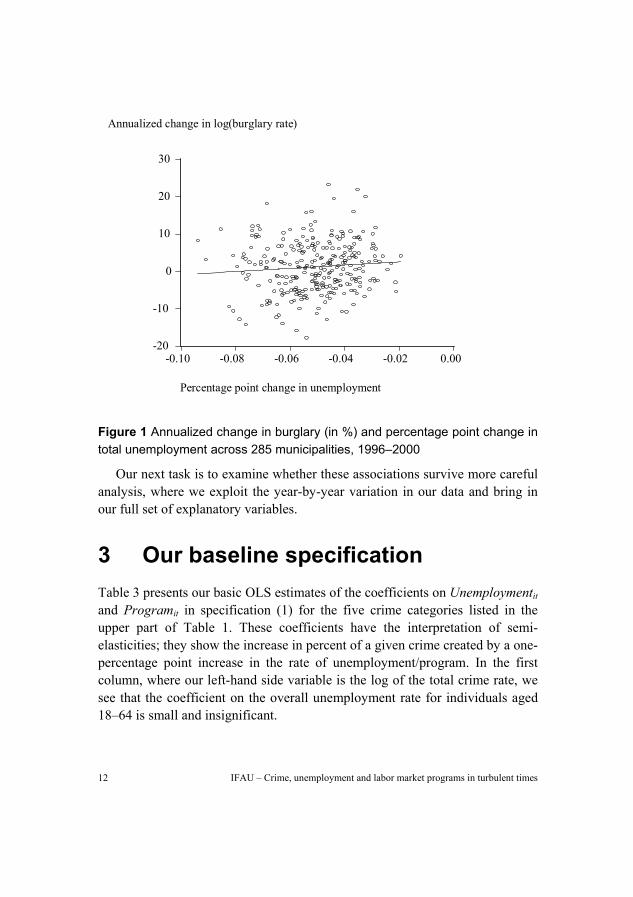
Figure 1 plots the change over the five-year period 1996–2000 in burglary per 100,000 residents against the reduction in overall unemployment across 285 municipalities. Two patterns stand out. First, there is indeed a huge variation across municipalities in the decrease in unemployment. Second, the plot is quite disperse, and it is not easy visually to detect a clear association between unemployment and the burglary rate. However, a simple OLS-regression shows that the slope coefficient on the change in unemployment is positive and significant at the seven-percent level. In a weighted OLS-regression, where we weigh all observations by the size of population, the slope coefficient becomes significant at the five-percent level.


12

-20

-10

0

10

20

30

-0.10 -0.08 -0.06 -0.04 -0.02 0.00

Percentage point change in unemployment

Annualized change in log(burglary rate)

Figure 1 Annualized change in burglary (in %) and percentage point change in total unemployment across 285 municipalities, 1996–2000

Our next task is to examine whether these associations survive more careful analysis, where we exploit the year-by-year variation in our data and bring in our full set of explanatory variables.

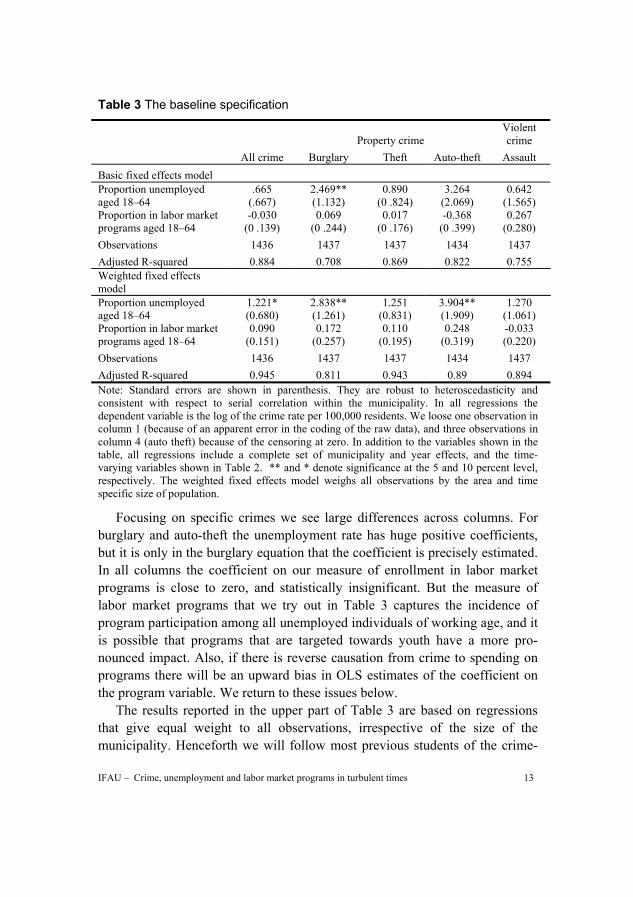
3 Our baseline specification Table 3 presents our basic OLS estimates of the coefficients on Unemploymentit and Programit in specification (1) for the five crime categories listed in the upper part of Table 1. These coefficients have the interpretation of semi-elasticities; they show the increase in percent of a given crime created by a one-percentage point increase in the rate of unemployment/program. In the first column, where our left-hand side variable is the log of the total crime rate, we see that the coefficient on the overall unemployment rate for individuals aged 18–64 is small and insignificant.


Table 3 The baseline specification

Property crime

Violent crime

All crime Burglary Theft Auto-theft Assault Basic fixed effects model Proportion unemployed aged 18–64

.665 (.667)

2.469** (1.132)

0.890 (0 .824)

3.264 (2.069)

0.642 (1.565)

Proportion in labor market programs aged 18–64

-0.030 (0 .139)

0.069 (0 .244)

0.017 (0 .176)

-0.368 (0 .399)

0.267 (0.280)

Observations 1436 1437 1437 1434 1437 Adjusted R-squared 0.884 0.708 0.869 0.822 0.755 Weighted fixed effects model Proportion unemployed aged 18–64

1.221* (0.680)

2.838** (1.261)

1.251 (0.831)

3.904** (1.909)

1.270 (1.061)


0.090 (0.151)

0.172 (0.257)

0.110 (0.195)

0.248 (0.319)

-0.033 (0.220)

Observations 1436 1437 1437 1434 1437 Adjusted R-squared 0.945 0.811 0.943 0.89 0.894 Note: Standard errors are shown in parenthesis. They are robust to heteroscedasticity and consistent with respect to serial correlation within the municipality. In all regressions the dependent variable is the log of the crime rate per 100,000 residents. We loose one observation in column 1 (because of an apparent error in the coding of the raw data), and three observations in column 4 (auto theft) because of the censoring at zero. In addition to the variables shown in the table, all regressions include a complete set of municipality and year effects, and the time-varying variables shown in Table 2. ** and * denote significance at the 5 and 10 percent level, respectively. The weighted fixed effects model weighs all observations by the area and time specific size of population.

Focusing on specific crimes we see large differences across columns. For burglary and auto-theft the unemployment rate has huge positive coefficients, but it is only in the burglary equation that the coefficient is precisely estimated. In all columns the coefficient on our measure of enrollment in labor market programs is close to zero, and statistically insignificant. But the measure of labor market programs that we try out in Table 3 captures the incidence of program participation among all unemployed individuals of working age, and it is possible that programs that are targeted towards youth have a more pro-nounced impact. Also, if there is reverse causation from crime to spending on programs there will be an upward bias in OLS estimates of the coefficient on the program variable. We return to these issues below.

The results reported in the upper part of Table 3 are based on regressions that give equal weight to all observations, irrespective of the size of the municipality. Henceforth we will follow most previous students of the crime-


14

unemployment link and focus on the results from weighted regressions, which downplay the influence of small municipalities. The lower part shows the results when we weigh all observations by the area and time specific size of population. In all equations the coefficient on unemployment tends to be larger, at the same time that the t-ratios increase. The coefficient on the unemployment variable is significant at the five-percent level in the equations for burglary and auto-theft, and at the ten-percent level in the equation for all crimes. Like previous studies, we find that unemployment has a statistically insignificant effect on the main category of violent crime, assault. The program variable remains statistically insignificant in all columns, with a coefficient close to zero.

The estimated coefficients matter economically. According to our weighted fixed effect regressions a one-percentage point drop in unemployment causes (everything else held constant) reductions of 1.2 percent in overall crime, 2.8 percent in the burglary rate, and 3.9 percent in the auto-theft rate. Since the mean unemployment rate decreased with 5.1 percentage points (from 11.9 to 6.8 percent) between the years 1996 and 2000, our coefficients predict a decrease of 6.1 percent for overall crime, 14.5 percent for burglary and 19.9 percent for auto-theft.

4 Alternative specifications In this section we analyze whether the significant crime-unemployment relations that we identified in the previous section (i.e. those involving all crimes, burglary and auto-theft) remain as we estimate alternative models.

A first issue concerns crime-spillovers. We have so far ignored all spatial interactions between municipalities. It appears likely, however, that criminal activities are correlated across adjacent municipalities – a criminal may choose to live in one community while committing crime in a neighboring community. For example, in their study of crime against foreigners in Germany, Krueger and Pischke (1997) find strong evidence of spatial correlation in anti-foreigner crime rates. A structurally oriented way of dealing with spatial spillover effects is to add covariates from neighboring municipalities to the estimating equation. Rather than allowing for spatial interactions via a transformation of the error term along the lines of e.g. Anselin (1988) – a procedure that has less obvious behavioral interpretations – we thus add new regressors to the estimating equation.


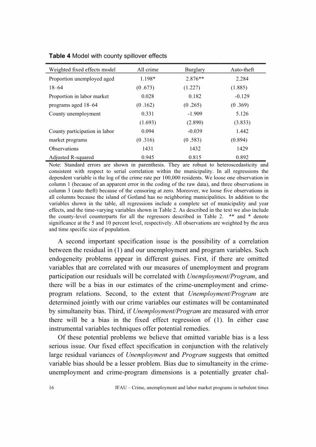
For each municipality we have constructed average (population-weighted) measures for all explanatory variables in the surrounding county, and then included these as additional regressors.13 The results from these extended regressions are shown in Table 4, which should be compared to our benchmark results of Table 3 (bottom panel). In the equations for all crimes and burglary the coefficient on municipality unemployment changes little as we include county spillovers, and the same holds true for the reported standard errors. As a consequence municipality unemployment remains a statistically significant determinant of all crimes and burglary. In these equations the county unemployment variable is very imprecisely estimated, with t-values of .2 (all crimes) and .66 (burglary). In the equation for auto-theft the coefficient on municipality unemployment drops from 3.904 to 2.284, and the standard error changes marginally, which implies that the t-value drops from 2.05 to 1.21. The estimated coefficient on county unemployment is large (5.126), though imprecisely measured. An F-test shows that the two unemployment variables in the equation for auto-theft are jointly significant at the ten-percent level (p-value = .09).

13 There are 21 counties in Sweden. Since the municipality coincides with the county for the island of Gotland, we could not create covariates from neighboring localities for this island. Hence, in Table 4 we loose five observations compared to Table 3.


16

Table 4 Model with county spillover effects

Weighted fixed effects model All crime Burglary Auto-theft Proportion unemployed aged 18–64

1.198* (0 .673)

2.876** (1.227)

2.284 (1.885)


0.028 (0 .162)

0.182 (0 .265)

-0.129 (0 .369)

County unemployment 0.331 -1.909 5.126 (1.693) (2.890) (3.833) County participation in labor market programs

0.094 (0 .316)

-0.039 (0 .583)

1.442 (0.894)

Observations 1431 1432 1429 Adjusted R-squared 0.945 0.815 0.892 Note: Standard errors are shown in parenthesis. They are robust to heteroscedasticity and consistent with respect to serial correlation within the municipality. In all regressions the dependent variable is the log of the crime rate per 100,000 residents. We loose one observation in column 1 (because of an apparent error in the coding of the raw data), and three observations in column 3 (auto theft) because of the censoring at zero. Moreover, we loose five observations in all columns because the island of Gotland has no neighboring municipalities. In addition to the variables shown in the table, all regressions include a complete set of municipality and year effects, and the time-varying variables shown in Table 2. As described in the text we also include the county-level counterparts for all the regressors described in Table 2. ** and * denote significance at the 5 and 10 percent level, respectively. All observations are weighted by the area and time specific size of population.

A second important specification issue is the possibility of a correlation between the residual in (1) and our unemployment and program variables. Such endogeneity problems appear in different guises. First, if there are omitted variables that are correlated with our measures of unemployment and program participation our residuals will be correlated with Unemployment/Program, and there will be a bias in our estimates of the crime-unemployment and crime-program relations. Second, to the extent that Unemployment/Program are determined jointly with our crime variables our estimates will be contaminated by simultaneity bias. Third, if Unemployment/Program are measured with error there will be a bias in the fixed effect regression of (1). In either case instrumental variables techniques offer potential remedies.

Of these potential problems we believe that omitted variable bias is a less serious issue. Our fixed effect specification in conjunction with the relatively large residual variances of Unemployment and Program suggests that omitted variable bias should be a lesser problem. Bias due to simultaneity in the crime-unemployment and crime-program dimensions is a potentially greater chal-


lenge. In a municipality where crime is rising there might be an induced outflow of firms and jobs, which increases unemployment. There will then be a causal and positive link from crime to unemployment, which will generate an upward bias in our OLS estimate of the coefficient on the unemployment variable.14 Whether there is reverse causation in the crime-program dimension depends on the decision rule of the labor market authorities. Dahlberg and Forslund (1999) argue that the National Labor Market Board allocates resources among regional authorities according to a rule saying that spending increases with past unemployment, and with past number of participants in programs. In the next stage of the decision process, when regional authorities allocate resources among municipalities, there does not appear to be any formalized allocation procedures, and concerns about crime might conceivably play a role. To the extent that a local crime shock generates increased spending on programs the OLS results reported in previous sections suffer from an upward bias; this may explain why we were unable to identify the predicted negative coefficient on the program variable.

Finally, in constructing our unemployment variable we had to invoke a measure of the total population of working age rather than a more appealing measure of the labor force. Under certain assumptions this measurement error will create a bias towards zero in our estimate of the coefficient on our unemployment variable. Since reverse causation from crime to unemployment can be expected to create an upward bias in the same coefficient, the overall bias can go either way.

We adopt an instrumental variables approach to address these issues. We derive our instruments for the unemployment variable following Blanchard and Katz (1992); i.e. we interact the first and second lags of municipality-level employment composition with the national trend in industrial growth to obtain two measures of the change in labor demand in different municipalities (see Appendix). In deriving our instruments for the program variable we follow Dahlberg and Forslund (1999) in assuming that lagged unemployment and lagged placement in labor market programs approximate the decision rule of labor market authorities. This gives us four instruments for our two labor

14 While we acknowledge that this bias is a theoretical possibility, we believe that it is bound to be small in practice. As indicated in our introduction, the huge variation in Swedish unemploy-ment during the 1990s can be traced to macroeconomic shocks that are exogenous to the municipality.


18

market variables. In the first stage regressions of our unemployment and program variables on our instruments (and our other controls, including the fixed municipality and time effects), the latter are jointly statistically significant at the .0000 level.15

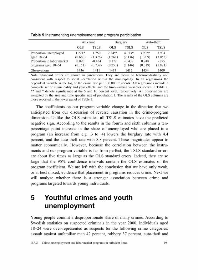
Table 5 presents our 2SLS estimates of the coefficients on the unemployment and program variables, along with the OLS estimates. The TSLS coefficients on the unemployment variable are generally larger than the OLS counterparts; in the equations for all crimes and burglary the TSLS coefficients are some 42–45 percent larger. We view this as evidence that our OLS estimates of the previous section do not exaggerate the impact of unem-ployment on crime. We obtained further support for this conclusion in TSLS regressions where we dropped lagged unemployment and lagged placement from the instrument set; in these specifications the TSLS estimates were more than three times as large as the OLS estimates. Finally, it should be noted that the TSLS standard errors are 60–100 percent larger than the OLS standard errors.

15 A test for the joint significance of our four instruments in the first stage unemployment regression produces an F-statistic of 151.11 (p-value = .0000). In the first stage program regression the F-statistic is 12.05 (p-value = .0000). Below we also report results when we only instrument the unemployment variable. In this regression we only use our labor demand shifters as instruments (i.e. we drop lagged unemployment and lagged program placement from the instrument set); the F-statistic for the joint significance of the two labor demand shifters in the first stage regression is 17.8 (p-value .0000). In assessing the credibility of our TSLS results it is important to test our overidentifying restrictions (we have more instruments than endogenous variables). We have regressed the TSLS residuals on all our exogenous variables, and tested for the joint statistical significance of our instrument set. In all these regressions, we failed to reject the null that our instruments are uncorrelated with the residuals.


Table 5 Instrumenting unemployment and program participation

All crime Burglary Auto-theft

OLS TSLS OLS TSLS OLS TSLS Proportion unemployed aged 18–64

1.221* (0.680)

1.750 (1.376)

2.84** (1.261)

4.033* (2.136)

3.90** (1.909)

3.934 (3.055)


0.090 (0.151)

-0.434 (0.739)

0.172 (0.257)

-0.437 (1.146)

0.248 (0.319)

-.875 (1.821)

Observations 1436 1411 1437 1412 1434 1409 Note: Standard errors are shown in parenthesis. They are robust to heteroscedasticity and consistent with respect to serial correlation within the municipality. In all regressions the dependent variable is the log of the crime rate per 100,000 residents. All regressions include a complete set of municipality and year effects, and the time-varying variables shown in Table 2. ** and * denote significance at the 5 and 10 percent level, respectively. All observations are weighted by the area and time specific size of population. I. The results of the OLS columns are those reported in the lower panel of Table 3.

The coefficients on our program variable change in the direction that we anticipated from our discussion of reverse causation in the crime-program dimension. Unlike the OLS estimates, all TSLS estimates have the predicted negative sign. According to the results in the fourth and sixth columns a ten-percentage point increase in the share of unemployed who are placed in a program (an increase from e.g. .3 to .4) lowers the burglary rate with 4.4 percent, and the auto-theft rate with 8.8 percent. These magnitudes appear to matter economically. However, because the correlation between the instru-ments and our program variable is far from perfect, the TSLS standard errors are about five times as large as the OLS standard errors. Indeed, they are so large that the 95% confidence intervals contain the OLS estimates of the program coefficient. We are left with the conclusion that we have only weak, or at best mixed, evidence that placement in programs reduces crime. Next we will analyze whether there is a stronger association between crime and programs targeted towards young individuals.

5 Youthful crimes and youth unemployment

Young people commit a disproportionate share of many crimes. According to Swedish statistics on suspected criminals in the year 2000, individuals aged 18–24 were over-represented as suspects for the following crime categories: assault against unfamiliar man 42 percent, robbery 37 percent, auto-theft and


20

drug possession 32 percent, burglary 31 percent and damage crime 29 percent.16 If we broaden the age category to 15–24, the percentages increase to 69 percent (robbery), 60 percent (assault against unfamiliar man), 57 percent (auto-theft), 51 percent (damage crime), 49 percent (burglary) and 37 percent (drug possession). Some studies suggest that labor market outcomes are of particular importance for the criminal activities of young people. Grogger (1998) reports estimates – based on longitudinal survey data for the U.S. – suggesting that falling real wages may have been an important determinant of rising youth crime during the 1970s and 1980s. Lochner and Moretti (2001) use a mix of individual and aggregate data, and show that high school graduation significantly reduces crime. They argue that this result to a large extent reflects the fact that education increases earnings, which increases the opportunity cost of crime.

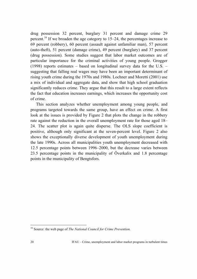
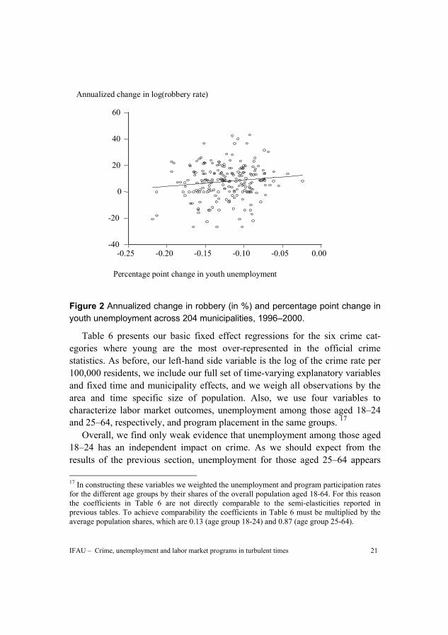
This section analyzes whether unemployment among young people, and programs targeted towards the same group, have an effect on crime. A first look at the issues is provided by Figure 2 that plots the change in the robbery rate against the reduction in the overall unemployment rate for those aged 18–24. The scatter plot is again quite disperse. The OLS slope coefficient is positive, although only significant at the seven-percent level. Figure 2 also shows the exceptionally diverse development of youth unemployment during the late 1990s. Across all municipalities youth unemployment decreased with 12.5 percentage points between 1996–2000, but the decrease varies between 23.5 percentage points in the municipality of Överkalix and 1.8 percentage points in the municipality of Bengtsfors.

16 Source: the web page of The National Council for Crime Prevention.


-40

-20

0

20

40

60

-0.25 -0.20 -0.15 -0.10 -0.05 0.00

Percentage point change in youth unemployment

Annualized change in log(robbery rate)

Figure 2 Annualized change in robbery (in %) and percentage point change in youth unemployment across 204 municipalities, 1996–2000.

Table 6 presents our basic fixed effect regressions for the six crime cat-egories where young are the most over-represented in the official crime statistics. As before, our left-hand side variable is the log of the crime rate per 100,000 residents, we include our full set of time-varying explanatory variables and fixed time and municipality effects, and we weigh all observations by the area and time specific size of population. Also, we use four variables to characterize labor market outcomes, unemployment among those aged 18–24 and 25–64, respectively, and program placement in the same groups. 17

Overall, we find only weak evidence that unemployment among those aged 18–24 has an independent impact on crime. As we should expect from the results of the previous section, unemployment for those aged 25–64 appears 17 In constructing these variables we weighted the unemployment and program participation rates for the different age groups by their shares of the overall population aged 18-64. For this reason the coefficients in Table 6 are not directly comparable to the semi-elasticities reported in previous tables. To achieve comparability the coefficients in Table 6 must be multiplied by the average population shares, which are 0.13 (age group 18-24) and 0.87 (age group 25-64).


22

with positive and statistically significant coefficients in the equations for auto-theft and burglary. We also identify a significant positive coefficient in the equation for drug possession. These effects remain as we estimate alternative models that instruments our labor market variables along the lines discussed in the previous section. But we estimate the coefficients on the youth unemploy-ment rate with much lower precision. In the equation for assault on unfamiliar man (this violent crime category includes various forms of street violence, where young men are heavily over-represented both among victims and perpetrators) we estimate a negative18, and marginally significant, coefficient on unemployment for those aged 18–24. The other borderline case is in the robbery equation, where the coefficient on the youth unemployment variable is positive and economically significant,19 with a p-value of .12. But in our instrumental variables regressions both coefficients change sign, and the t-values drop to 0.60 and 0.67.

18 Both Raphael and Winter-Ebmer (2001) and Gould, Weinberg and Mustard (2002) report that state- and county-level unemployment have a negative impact on some categories of violent crime in the U.S. Raphael and Winter-Ebmer report evidence that this is due to a lower frequency of interactions between victims and perpetrators when unemployment is high. 19 Multiplying the coefficient of 16.1 with a population share of 0.13 (see footnote 17) produces a semi-elasticity of 2.1, which is of a magnitude that matters economically. It implies that a one-percentage point increase in unemployment among males aged 18-24 increases the robbery rate with 2.1 percent. Since the unemployment rate of those aged 18-24 decreased with 12.5 percentage points between 1996–2000, our estimate predicts a decrease in the robbery rate with 26.3 percent over the same period.

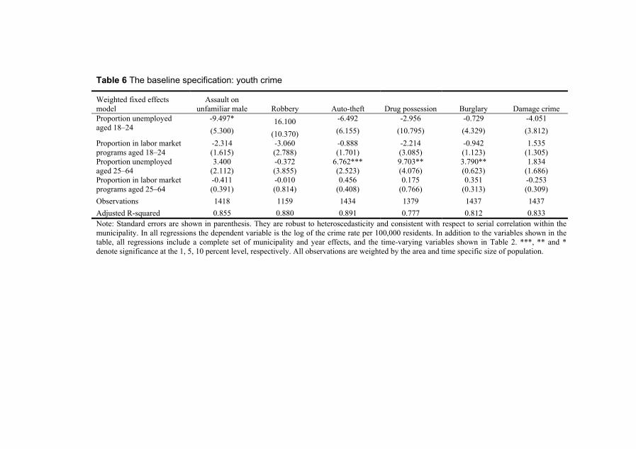
Table 6 The baseline specification: youth crime

Weighted fixed effects model

Assault on unfamiliar male Robbery Auto-theft Drug possession Burglary Damage crime

Proportion unemployed aged 18–24

-9.497* (5.300)

16.100 (10.370)

-6.492 (6.155)

-2.956 (10.795)

-0.729 (4.329)

-4.051 (3.812)


-2.314 (1.615)

-3.060 (2.788)

-0.888 (1.701)

-2.214 (3.085)

-0.942 (1.123)

1.535 (1.305)


3.400 (2.112)

-0.372 (3.855)

6.762*** (2.523)

9.703** (4.076)

3.790** (0.623)

1.834 (1.686)


-0.411 (0.391)

-0.010 (0.814)

0.456 (0.408)

0.175 (0.766)

0.351 (0.313)

-0.253 (0.309)

Observations 1418 1159 1434 1379 1437 1437 Adjusted R-squared 0.855 0.880 0.891 0.777 0.812 0.833 Note: Standard errors are shown in parenthesis. They are robust to heteroscedasticity and consistent with respect to serial correlation within the municipality. In all regressions the dependent variable is the log of the crime rate per 100,000 residents. In addition to the variables shown in the table, all regressions include a complete set of municipality and year effects, and the time-varying variables shown in Table 2. ***, ** and * denote significance at the 1, 5, 10 percent level, respectively. All observations are weighted by the area and time specific size of population.

24 IFAU – Crime, unemployment and labor market programs in turbulent times

With one exception the coefficients on program participation for those aged 18–24 are estimated with the predicted negative sign. But the point estimates are numerically small, with t-ratios at, or below, unity. Transforming the coefficients into semi-elasticities (see footnote 17), the latter lie in an interval between -0.39 (robbery) and 0.02 (damage crime). In our instrumental variables regressions, where we model the decision rule of the labor market authorities in the manner of the previous section, all standard errors increase substantially, while the point estimates either stay about the same, or change sign from negative to positive.

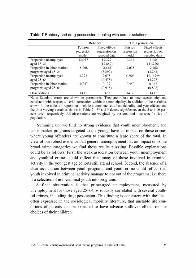
A final unresolved issue derives from the fact that some youth crimes have an incidence of zero in many municipalities. Because of our logarithmic transformation these observations become missing values in Table 6. This implies that we lose close to 20 percent of the observations in the equation for robbery, and 4 percent of the observations for drug possession. To see whether this censoring matters for our results we estimate two alternative models. First, since the incidence of crimes per 100,000 residents is measured on a scale that only takes on non-negative integer values, our left-hand side variable is a count variable. Because of this we estimate a Poisson regression model, using our full sample. Second, we simply re-code all zeros to ones, before introducing the logarithmic transformation of our left-hand side variable, and then estimating our baseline fixed effect model. In either case, we are left with a full sample of 1437 observations. The results are shown in Table 7.20 It does not appear that censoring is an important issue. Comparing with the results for robbery and drug possession in Table 6, the order of magnitude of the coefficients remains the same. Also, in both tables it is only in the equation for drug possession that we identify a statistically significant coefficient, the one on unemployment for those aged 25–64.

20 It should be noted that because of the logarithmic transformation used in the baseline model, the estimated coefficients in the Poisson model are comparable to those presented in Table 6.We do not report the standard errors in our Poisson regressions. These standard errors are defined by the conditional mean of the dependent variable, which is a poor assumption.


Table 7 Robbery and drug possession: dealing with corner solutions

Robbery Drug possession

Poisson regression

model

Fixed effects regression on recoded data

Poisson regression

model

Fixed effects regression on recoded data


13.927 19.329 (12.859)

-0.344 -1.085 (11.220)


-5.008 -2.648 (3.899)

-7.035 -2.262 (3.262)


3.322 2.078 (4.478)

5.605 10.149** (4.297)


-0.247 0.137 (0.915)

-0.450 0.142 (0.808)

Observations 1437 1437 1437 1437 Note: Standard errors are shown in parenthesis. They are robust to heteroscedasticity and consistent with respect to serial correlation within the municipality. In addition to the variables shown in the table, all regressions include a complete set of municipality and year effects, and the time-varying variables shown in Table 2. ** and * denote significance at the 5 and 10 per-cent level, respectively. All observations are weighted by the area and time specific size of population.

Summing up, we find no strong evidence that youth unemployment, and labor market programs targeted to the young, have an impact on those crimes where young offenders are known to constitute a large share of the total. In view of our robust evidence that general unemployment has an impact on some broad crime categories we find these results puzzling. Possible explanations could be as follows. First, the weak association between youth unemployment and youthful crimes could reflect that many of those involved in criminal activity in the youngest age cohorts still attend school. Second, the absence of a clear association between youth programs and youth crime could reflect that youth involved in criminal activity manage to opt out of the programs; i.e. there is a selection of non-criminal youth into programs.

A final observation is that prime-aged unemployment, measured by unemployment for those aged 25–64, is robustly correlated with several youth-ful crimes, including drug possession. This finding is consistent with the idea, often expressed in the sociological mobility literature, that unstable life con-ditions of parents can be expected to have adverse spillover effects on the choices of their children.


6 Conclusions A main advantage of our study is that we have access to a data set – gathered from a period with extraordinary shocks to local unemployment – that sub-stantially reduces the risk that omitted variables and reverse causation lead to biased estimates of the crime-unemployment relationship. During the time period under investigation the changes in local unemployment were much larger than the changes in other plausible determinants of crime, and the origin of these shocks to unemployment can be traced to macroeconomic events, external to the municipality.

Our main results can be summarized as follows. First, even in a welfare state where social insurance cushions a substantial part of the income loss from job displacement, a shock to general unemployment has a statistically and economically significant impact on main categories of property crime. Second, we could not establish a clear association between youth unemployment and the incidence of certain youthful crimes. Some of these crimes are, however, correlated with prime-aged unemployment, a finding that points towards the possible role of parental economic conditions in determining youth crime.

Third, we found little evidence that labor market programs reduce crime. Though we found some weak evidence that programs targeted towards the general population of unemployed reduce property crime, we found no indications at all that programs targeted towards those aged 18–24 have an impact. Our data does not allow us to tell whether this non-association reflects a true behavioral response, or whether it primarily reflects a selection process, where criminally inclined young individuals are sorted into non-participation. In view of the large sums spent on these programs, it seems appropriate to conclude with the customary call for future research.


References Anselin, L. (1988), Spatial econometrics: Methods and Models, Kluwer Academic, Dordrecht.

Becker, G (1968), Crime and punishment: an economic approach, Journal of Political Economy 76, 169–217.

Blanchard, O. J. and L. F. Katz (1992), Regional evolutions, Brookings Papers on Economic Activity (issue 1), 1–61.

Calmfors, L., A. Forslund and M. Hemström (2002), Does active labor market policy work? Lessons from the Swedish Experience, IFAU Working Paper 2002:4. Chiricos, T (1987), Rates of crime and unemployment: an analysis of aggregate research evidence, Social Problems 34, 187–212.

Dahlberg, M. and A. Forslund (1999), Direct displacement effects of labor market programmes: the case of Sweden, IFAU Working Paper 1999:7.

Edmark, K (2002), Arbetslöshetens effekter på brottsligheten, Ekonomisk Debatt 30, 403–416. Freeman, R. (1996), Why do so many young American men commit crimes and what might we do about it?, Journal of Economic Perspectives 10, 25–42.

Freeman, R. (1999), The economics of crime, in Handbook of Labor Economics, vol. 3C (eds. Ashenfelter, O. C. and Card, D.), Elsevier, Amsterdam. Gould, E., B. Weinberg and D Mustard (2002), Crime rates and local labor market opportunities in the United States: 1979–1997, Review of Economics and Statistics 84, 45–61.


le Grand, C. (1986), Kriminalitet och arbetsmarknad; inklusive en tidsserieanalys av inbrottsfrekvensen 1950–1977, Institutet för social forskning, Stockholms universitet. Grogger, J (1998), Market wages and youth crime, Journal of Labor Economics 16, 756–791.

Kézdi, G. (2002), Robust standard error estimation in fixed-effects panel models, mimeo, University of Michigan.

Krueger, A. and J.-S. Pischke (1997), A statistical analysis of crime against foreigners in unified Germany, Journal of Human Resources 34, 182–209.

Levitt, S. D (1997), Using electoral cycles in police hiring to estimate the effect of police on crime, American Economic Review 87, 270–290.

Lindbeck, A. (1997), The Swedish experiment, Journal of Economic Literature 35, 1273–1319. Lochner, L. and E. Moretti (2001), The effect of education on crime: evidence from prison inmates, arrests, and self-reports, NBER Working Paper No. 8605.

Machin S. and C. Meghir (2000), Crime and economic incentives, The Institute for Fiscal Studies, Working Paper 00/17. National Council for Crime Prevention (2001), Brottsutvecklingen i Sverige 1998–2000, BRÅ-rapport 2001:10, Stockholm.

Raphael, S and R Winter-Ebmer (2001), Identifying the effect of unemployment on crime, Journal of Law and Economics 41, 259–283. Schuller, B-J (1986), Ekonomi och kriminalitet – en empirisk undersökning av brottsligheten i Sverige, Ph.D.-dissertation, Department of Economics, University of Gothenburg.


Appendix 1: Definitions of variables

Table 8 Definitions of crime variables

Variables Definitions All crimes All crimes reported in the municipality during the year. Burglary All burglary, not including fire arms. Theft All thefts from vehicles, in public places, restaurants, shops, schools etc.

Also including shoplifting and pick pocketing. Auto theft All car thefts, both attempted and completed. Assault All assaults, not with fatal ending, against children, women and men. Assault against male, unfamiliar with the victim

Assault against male where the perpetrator is unfamiliar with the victim, both outdoors and indoors.

Damage crime All damage crime, including graffiti. Robbery All robbery against the person. Possession of drugs Including possession of drugs and own usage. Note: All variables are number of crimes reported to the police per 100,000 inhabitants.

Table 9 Definitions of control variables

Variables Definitions Proportion unemployed aged 18–64, 18–24 and 25–64.

Number of unemployed individuals out of total population in relevant age-group.

Proportion unemployed in labor market programs, aged 18–64, 18–24 and 25–64.

Number of individuals in labor market programs out of total number of unemployed individuals in relevant age-group.

Proportion not born in Sweden Number of individuals not born in Sweden out of total population. Income per capita (in kronor) Taxable income per capita. Age distribution Proportion of individuals in different age-groups out of total

population. Proportion of men Number of men out of total population. Proportion with no high-school degree Proportion of the population with at most nine years of schooling.

Proportion with high school degree Proportion with between 10 and 12 years of schooling.

Appendix 2: Results for the baseline specification

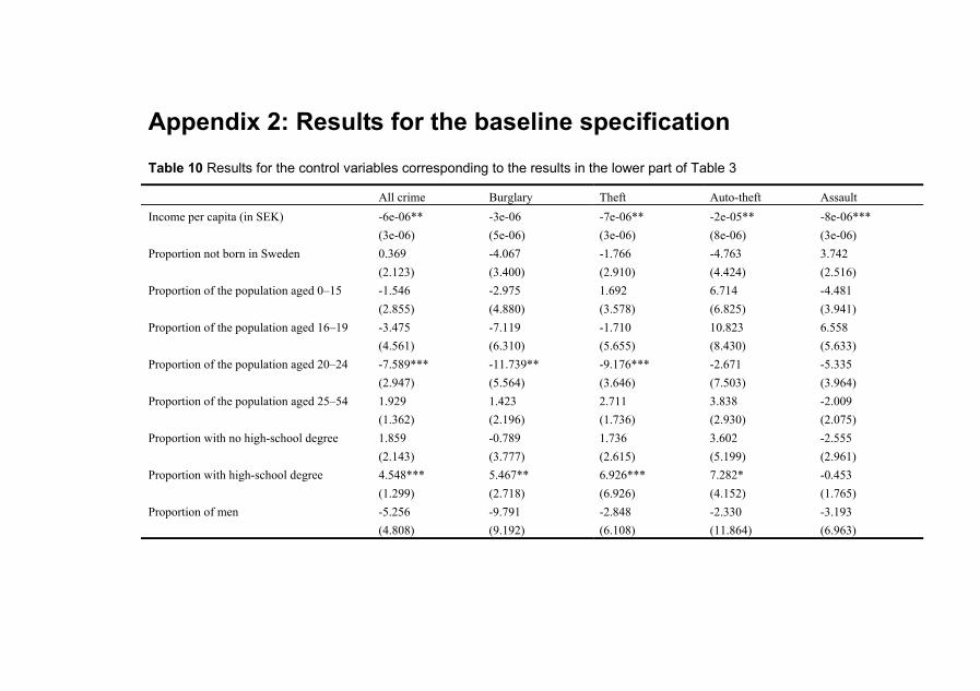
Table 10 Results for the control variables corresponding to the results in the lower part of Table 3

All crime Burglary Theft Auto-theft Assault Income per capita (in SEK) -6e-06** -3e-06 -7e-06** -2e-05** -8e-06*** (3e-06) (5e-06) (3e-06) (8e-06) (3e-06) Proportion not born in Sweden 0.369 -4.067 -1.766 -4.763 3.742 (2.123) (3.400) (2.910) (4.424) (2.516) Proportion of the population aged 0–15 -1.546 -2.975 1.692 6.714 -4.481 (2.855) (4.880) (3.578) (6.825) (3.941) Proportion of the population aged 16–19 -3.475 -7.119 -1.710 10.823 6.558 (4.561) (6.310) (5.655) (8.430) (5.633) Proportion of the population aged 20–24 -7.589*** -11.739** -9.176*** -2.671 -5.335 (2.947) (5.564) (3.646) (7.503) (3.964) Proportion of the population aged 25–54 1.929 1.423 2.711 3.838 -2.009 (1.362) (2.196) (1.736) (2.930) (2.075) Proportion with no high-school degree 1.859 -0.789 1.736 3.602 -2.555 (2.143) (3.777) (2.615) (5.199) (2.961) Proportion with high-school degree 4.548*** 5.467** 6.926*** 7.282* -0.453 (1.299) (2.718) (6.926) (4.152) (1.765) Proportion of men -5.256 -9.791 -2.848 -2.330 -3.193 (4.808) (9.192) (6.108) (11.864) (6.963)


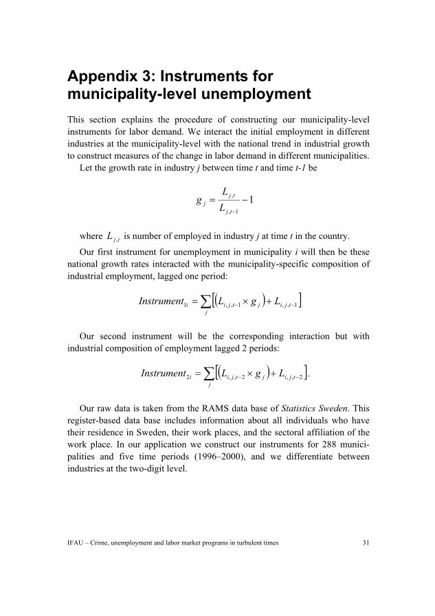
Appendix 3: Instruments for municipality-level unemployment This section explains the procedure of constructing our municipality-level instruments for labor demand. We interact the initial employment in different industries at the municipality-level with the national trend in industrial growth to construct measures of the change in labor demand in different municipalities.

Let the growth rate in industry j between time t and time t-1 be

11,

, −=−tj

tjj L

Lg

where tjL , is number of employed in industry j at time t in the country.

Our first instrument for unemployment in municipality i will then be these national growth rates interacted with the municipality-specific composition of industrial employment, lagged one period:

( )[ ]∑ −− +×=

jtjijtjii LgLInstrument 1,,1,,1

Our second instrument will be the corresponding interaction but with

industrial composition of employment lagged 2 periods:

( )[ ]∑ −− +×=j

tjijtjii LgLInstrument 2,,2,,2 .

Our raw data is taken from the RAMS data base of Statistics Sweden. This

register-based data base includes information about all individuals who have their residence in Sweden, their work places, and the sectoral affiliation of the work place. In our application we construct our instruments for 288 munici-palities and five time periods (1996–2000), and we differentiate between industries at the two-digit level.

Publication series published by the Institute for Labour Market Policy Evaluation (IFAU) – latest issues Rapport

2003:1 Mörk Eva ”De arbetsmarknadspolitiska progammens effekt på den kommu-nala skolan”

2003:2 Runeson Caroline & Anders Bergeskog ”Arbetsmarknadspolitisk översikt 2000”

2003:3 Runeson Caroline & Anders Bergeskog ”Arbetsmarknadspolitisk översikt 2001”

2003:4 Calleman Catharina ”Invandrarna, skyddet för anställningen och diskrimine-ringslagstiftningen”

2003:5 Rooth Dan-Olof & Olof Åslund ”Spelar när och var någon roll? Arbets-marknadslägets betydelse för invandrares inkomster”

2003:6 Forslund Anders & Bertil Holmlund ”Arbetslöshet och arbetsmarknads-politik”

2003:7 Fröberg Daniela, Linus Lindqvist, Laura Larsson, Oskar Nordström Skans & Susanne Ackum Agell ”Friåret ur ett arbetsmarknadsperspektiv – del- rapport 1”

2003:8 Olofsson Jonas ”Grundläggande yrkesutbildning och övergången skola arbetsliv – en jämförelse mellan olika utbildningsmodeller”

2003:9 Olli Segendorf Åsa ”Arbetsmarknadspolitiskt kalendarium II”

2003:10 Martinson Sara & Martin Lundin ”Vikten av arbetsgivarkontakter: en studie av den yrkesinriktade arbetsmarknadsutbildningen i ljuset av 70-procentsmålet”

Working Paper

2003:1 Fredriksson Peter & Per Johansson “Program evaluation and random pro-gram starts”

2003:2 Mörk Eva “The impact of active labor market programs on municipal ser-vices”

2003:3 Fredriksson Peter & Per Johansson “Employment, mobility, and active labor market programs”

2003:4 Heckman James & Salvador Navarro-Lozano “Using matching, instrumental variables and control functions to estimate economic choice models”

2003:5 Fredriksson Peter & Bertil Holmlund “Improving incentives in unemploy-ment insurance: A review of recent research”

2003:6 Lindgren Urban & Olle Westerlund “Labour market programmes and geo-graphical mobility: migration and commuting among programme partici-pants and openly unemployed”

2003:7 Åslund Olof & Dan-Olof Rooth “Do when and where matter? Initial labor market conditions and immigrant earnings”

2003:8 Håkanson Christina, Satu Johanson & Erik Mellander “Employer-sponsored training in stabilisation and growth policy perspectives”

2003:9 Carneiro Pedro, Karsten Hansen & James Heckman “Estimating distribu-tions of treatment effects with an application to the returns to schooling and measurement of the effects of uncertainty on college choice”

2003:10 Heckman James & Jeffrey Smith “The determinants of participation in a social program: Evidence from at prototypical job training program”

2003:11 Skedinger Per & Barbro Widerstedt “Recruitment to sheltered employment: Evidence from Samhall, a Swedish state-owned company”

2003:12 van den Berg Gerard J & Aico van Vuuren “The effect of search frictions on wages”

2003:13 Hansen Karsten, James Heckman & Kathleen Mullen “The effect of school-ing and ability on achievement test scores”

2003:14 Nilsson Anna & Jonas Agell “Crime, unemployment and labor market pro-grams in turbulent times”

Dissertation Series

2002:1 Larsson Laura “Evaluating social programs: active labor market policies and social insurance”

2002:2 Nordström Skans Oskar “Labour market effects of working time reductions and demographic changes”

2002:3 Sianesi Barbara “Essays on the evaluation of social programmes and educa-tional qualifications”

2002:4 Eriksson Stefan “The persistence of unemployment: Does competition between employed and unemployed job applicants matter?”

2003:1 Andersson Fredrik “Causes and labor market consequences of producer heterogeneity”

Documents

Annals of Economics and Finance - down.aefweb.netdown.aefweb.net/AefArticles/aef150209Nilsson.pdf · IFAU – Crime, unemployment and labor market programs in turbulent times 1 Crime,