ANM 2.1 site documentationanm.csb.pitt.edu/anmdocs/ANM2.1_Documentation.pdf · ANM (Anisotropic network model) is a simple NMA tool for analysis of vibrational motions in molecular

18.9.2016 anm.csb.pitt.edu/anmdocs/Documentation2.1.html

http://anm.csb.pitt.edu/anmdocs/Documentation2.1.html 1/17

ANM 2.1 site documentationDownload the documentation pages in PDF

Theory

Manual

Submission page

Applicability

Software used

Input parameters

Advanced Input Options

Output text files

Output coordinate files

Using the graphical interface

Known problems and possible solutions

References

Theory

ANM (Anisotropic network model) is a simple NMA tool for analysis of vibrational motions in molecularsystems introduced in 2000 (1,2). It uses Elastic Network (EN) methodology and represents the system in the residue level. The macromolecule is thus represented as a network, or graph. In theoriginal model each protein node is the Cα atom of a residue and the overall potential is simply thesum of harmonic potentials between interacting nodes. The network includes all interactions within acutoff distance which is the only predetermined parameter in the model. Information about theorientation of each interaction with respect to the global coordinates system is considered within the

http://anm.csb.pitt.edu/anmdocs/ANM2.1_Documentation.pdf

http://anm.csb.pitt.edu/cgi-bin/anm2/anm2.cgi



Force constant matrix and allows prediction of anisotropic motions. The model wassuccessfully applied for exploring the relation between function and dynamics for many proteins (e.g.3,4,5). The force constant of the system can be described by a Hessian matrix:

(1)

Each element Hi,j is a 3×3 matrix which holds the anisotropic informations regarding the orientation of

nodes i,j. Each such sub matrix (or the "super element" of the Hessian) is defined as:

(2)

color namely the second partial derivatives of the potential V. These partial derivatives comprise asimple matrix of cosines. In practice the offdiagonal super elements are calculated by:



(3)

where γ is an interaction constant which taken as constant in the original ANM. si,j is the instantaneous

distance between nodes i and j.The diagonal super elements are calculated by:

(4)

Note that the force constant matrix H holds information regarding the orientation of the nodes, but notregarding the type of the interaction (such is whether the interaction is covalent or noncovalent,hydrophobic or nonhydrophobic, etc.). In addition, the distance between the interacting nodes is notconsidered directly. To account for the distance between the interactions we can weight eachinteraction between nodes i, j by the distance:

(5)

where p is an empirical parameter. The new offdiagonal elements of the Hessian matrix take the formof:

(6)



The inverse of the Hessian matrix is the covariance matrix of 3N multivariant Gaussian distributionwhich hold the desired information about the fluctuations. The Hessian, however is not invertible, as itsrank is 3N6 (6 variables responsible to a rigid body motion). To obtain a pseudo inverse, a solution tothe eigenvalue problem is obtained:

(7) The pseudo inverse is composed of the 3N6 eigenvectors and their respective nonzero eigen valuesaccording to:

(8)

Where λi are the eigenvalues of H sorted by their size from small to large and Ui the corresponding

eigenvectors. The eigenvectors (the columns of the matrix U) describe the vibrational direction and therelative amplitude in the different modes. The mean square fluctuations of individual residues can beobtained by summing the fluctuations in the individual modes as follows:

(9) The cross correlation between different residues can be also determined from the inverse Hessianmatrix:

(10)

For more advanced reading about the theory behind the model and its applications see references11,12.

Back to the top of the documentation page



Description of the web site

Applicability

The current version (ANM 2.1) of this web site is built to be used with proteins and nucleic acids. Otherligands which exist in the coordinates file may also be included. For proteins and nucleic acids the sitesuggests default nodes (Ca for amino acids, P, C4', C2 for nucleic acids), while for nontandard liagndsthe user need to manually chose nodes and interaction cutoffs if she wishes to include those in themodel. For full functionality, the size of the protein should be up to 1500 residues. For such structuresthe calculation of 20 dominant modes is performed within seconds. The calculation of the theoretical Bfactors based on all the modes is done within 2 minutes. The analysis pages could appear in a delay,depending on the communication speed and the memory of the client computer (downloading largeresult files to the user machine), but will not appear within more than a minute or two for suchmoderatesize proteins in any case. For larger proteins some problems with the graphics are expected.The calculation of the bfactors might take longer. The dominant modes calculation, however, will beperformed and text files with the results will still be available within few minutes. The site was testedwith proteins up to 2000 residues. For structures with more nodes expect functional problems. Note thatthe JSmol applet on the main interface page could be slow for large structures, as the coordinates file(which should include a frame for each normal mode) becomes huge and causing memory issues. Thegraphic pages that appears under the create PDB files option might behave better because onlyinformation about individual modes is saved in the memory at each time.The site was successfully tested on Windows10 and Windows7 using the following browsers:

FirefoxInternet ExplorerOperaGoogle Chrome

On Linux, using the following browsers:

FirefoxOperaGoogle Chrome

On MacOSX, using the following browsers:

Mozilla Firefox



Version 2.1 from Oct 2016 is different from version 2.0, which was described in the 2015 Bioinformaticsapplication note, by several techinal aspects, in particular the introduction of JSmol instead of Jmol forvisualization. This change makes the site much less platform and browser dependent. No externalinstallations of Java plugins is needed.

The eigensolvers

This site uses BLZPACK (6) and Matlab (9) for calculating a subset of eigenmodes. The default valueis 20 modes but this number can be changed in the input page. If the number of requested modes isdifferent than 20, the user should choose matlab as the eigensolver. The site calculates and report theslowest modes. BLZPACK is a Fortran 77 implementation of the block Lanczos algorithm for thesolution of the eigenvalue problems. It was originally intended to solve large, sparse, generalizedproblems which makes it very appropriate for the use here. In Matlab we use the eigs function which isthe Matlab interface to the ARPACK package. The server calculates a subset of the eigenpairs and notall of them. This is sufficient since we are usually interested in a small set of eigenpairs correspondingto the smallest eigenvalues ("slow modes"). The eigen decomposers use extremely efficient algorithms(6). For molecules with 300 residues (900×900 ANM Hessian matrix); the solution is obtained within 2seconds and for structures with thousands of nodes it is typically obtained within few minutes.

Jmol the molecular graphics tool

JSmol (7) is a free code molecular graphics tool which can be used in both HTML5 and Java modes. Itwas chosen to provide the graphics for this site as the code is actively and rapidly developed, andsince it was originally designed to support visualization of vibrations. This support includes the optionfor animation of all vibrational modes in one session with only button click required to switch betweenthe modes. Directional vectors can be presented for easy visualization of the direction of motion ateach mode. Anisotropic parameters, a direct product of the ANM results can also esaily displayedusing JSmol. Detailed documentation and description of JSmol capabilities are available on the Jmolsite. In general, many options can be controlled by the mouse from the pop up menu (right mouse clickon the applet). Other options are available by command line scripting language which is highlycompatible with the traditional RasMol scripting language (open the "console" option from the pop upmenu to execute commands). For several options which are directly related to the vibrations and forsome important visualization features we built a control panel for the user which will be described. We highly acknowledge the work done by the Jmol team that allow us (and other) to presentsophisticated data in a convenient and quality graphical environment.JSmol can be run in the HTML5 mode in essentially any platform and web browser. In recent years

http://crd-legacy.lbl.gov/~osni/marques.html#BLZPACK

http://www.mathworks.com/products/matlab/

http://jmol.sourceforge.net/

http://www.openrasmol.org/



several security problems with Java applets gradually limit the usgae of the Java mode in differentplatforms and browsers. We suggest here solutions to some of the problems.

Other software applied

Matlab (9) is also used for matrix manipulations and a fast calculation of theoretical Bfactors based onall the modes using the eig function. Perl modules are applied for cgi web programming and drawing ofgraphs and figures. C code is used for parsing of structures and calculation of the Hessian matrix. TheMatlab and Perl and the C codes are available upon request. The C codes for local ANM calculationsand constructions of Hessian matrix is available here.

Back to the top of the doumentation page

Input parameters

The minimal required input is very simple. The user should only specify an input coordinates' file in aPDB format. There are 2 ways to specify the file:

Specification of a 4 letter code PDB ID. The user can choose by a checkbox if to use theoriginal PDB coordinates (default) or the putative biological unit suppled by the PDB. The lattershould reflect better the biological multimeric state of the protein.

Uploading of a coordinates file from the user computer to the server.

The other input parameters are usually not required for a successful run. Still, they might be importantand relevant and influence the quality of the results: The user should determine if she wishes to include all polypeptides chains in the calculation (default) oronly individual chain. In the latter, a chain ID (usually a Latin letter A,B etc.) should be specified on theappropriate text field in the input page. An input chain symbols such as "*", " " , "", "_" , "0" will causeinclusion of all polypeptide chains in the calculation.

In addition, the user can define which models will be included in the calculation. Models are often (butnot always) used to include alternative conformations in the file. The two most frequent situations inwhich the coordinates file include different models are NMR files and files with the biological unitinformation. In the first case the user should choose which of the models in the file (usually marked asinteger numbers) should serve as the equilibrium state for the calculation. In the second case the usershould probably specify "all" in the text field for model as all the coordinates in the file (even those

http://anm.csb.pitt.edu/cgi-bin/anm2/Java_instructions.cgi

http://www.mathworks.com/

http://anm.csb.pitt.edu/anmdocs/source.html

http://www.rcsb.org/pdb/static.do?p=file_formats/pdb/index.html

http://www.rcsb.org/pdb/static.do?p=education_discussion/educational_resources/biounit_tutorial.html



found under different models) are part of one biological unit.

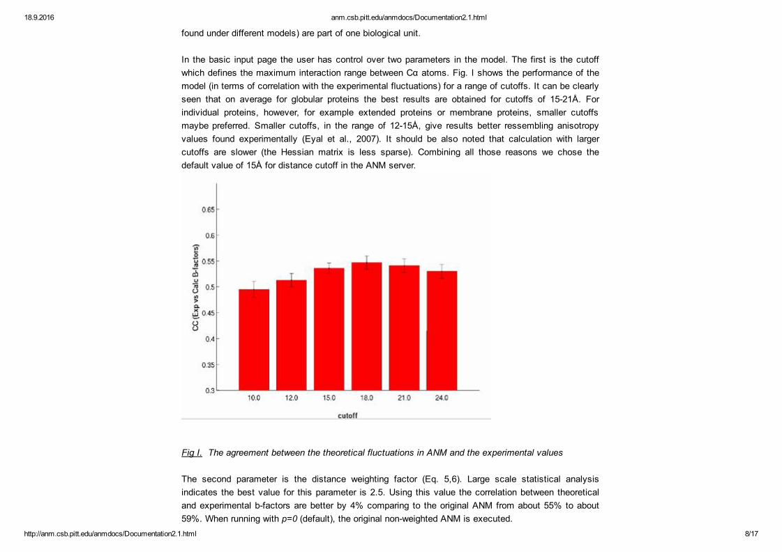
In the basic input page the user has control over two parameters in the model. The first is the cutoffwhich defines the maximum interaction range between Cα atoms. Fig. I shows the performance of themodel (in terms of correlation with the experimental fluctuations) for a range of cutoffs. It can be clearlyseen that on average for globular proteins the best results are obtained for cutoffs of 1521Å. Forindividual proteins, however, for example extended proteins or membrane proteins, smaller cutoffsmaybe preferred. Smaller cutoffs, in the range of 1215Å, give results better ressembling anisotropyvalues found experimentally (Eyal et al., 2007). It should be also noted that calculation with largercutoffs are slower (the Hessian matrix is less sparse). Combining all those reasons we chose thedefault value of 15Å for distance cutoff in the ANM server.

Fig I. The agreement between the theoretical fluctuations in ANM and the experimental values

The second parameter is the distance weighting factor (Eq. 5,6). Large scale statistical analysisindicates the best value for this parameter is 2.5. Using this value the correlation between theoreticaland experimental bfactors are better by 4% comparing to the original ANM from about 55% to about59%. When running with p=0 (default), the original nonweighted ANM is executed.



The "number of modes" parameter determines how many dominant normal modes will be calculated.More modes give more compleate picture on the dynamics of the system in the cost of computationaltime. 20 modes are usually sufficient to describe the important motions of smallmedium systems asthe slow modes are usually the functional ones.

The viewer parameter determines if JSmol will be applied in HTML5/Javascript mode (HTML5) or inJava mode. The HTML5 mode is more robust to platforms, browsers and does not require preinstallation of Java, however the Java mode gives slightly better graphics and perfomance when it canbe applied.

Advanced Input Options

Since version 2.0 of the ANM website, we allow now more sophisticated control over the runparameters. These optional parameters should be provided from the "Proceed with advanced inputoptions button" in the bottom of the input page. The user can control the identity of the atoms which willserve as nodes in the network. For proteins, the Cα atoms are the default nodes, but the user canchange to other backbone atoms if needed. For nucleic acids, the default setting is that eachnucleotide will be represented by 3 nodes. By default each nucleotide is represented in the network bythree nodes, positioned at the P atom of the phosphate group, C4' in the base and C2 in the sugar ring.This model has been shown (Yang et al., 2006) to have superior predictive abilities, based on thecomparison with experimental Bfactors using 64 oligonucleotide/protein complexes (13) and on casestudies such as the application of ANM to the ribosome (14). The server provides the option of adoptingdifferent number and types of userdefined atoms for representing the nucleotide nodes. All backboneheavy atoms of the protein and all the nuculeotide atom types are listed and can be selected as nodes.Small ligands can also be explicitly included in the ANM analysis. Ligands, if present in the PDBcoordinates file, will be automatically parsed and listed and their atoms will appear in separate a list.Each atom from this list can also be selected by the user as a network node.

To support the above changes, the server applies now a new strategy that enables flexibility in thedefinition of network nodes and cutoff distances of interaction. The cutoff, rc depends on the identity ofpotentially interacting atoms i, j. For each atom type i, an associated distance range of interaction, ti, is

assigned. For each pair of atom types i, j the cutoff distance rc is defined as ti+tj. This definition

implies that the number of parameters in the system is bound by the number of different atom types. Inthe simplest case where we want a unified threshold distance rc for all atom types, as in the traditionalANM, we simply assign ti = rc/2 for all atom types we would like to include. The server suggests rc=15



as default setting.

In the advanced input page the user has an additional option of importing external normal modes, e.g.submitting principal modes that have been calculated by another method, and take advantage of thepowerful GUI of the server for visualizing the motions and the crosscorrelations between residues. Thedimensions of these uploaded vectors must match the number of system nodes defined by the user.Thne user should upload 3 files, for the X,Y and Z components of the modes according to this format

Output text files

A series of text files which include the outcome of the calculation plus additional analyses are availablefor download:

Slow eigenvectors (oanm.slwevs) : List the eigen vectors which correspond to smallestN eigen values. N is the number of eigenvectors requested by the user on the input page.Snap

Slow Eigenvlaues (oanm.eigvals) : Lists the N smallest eigenvalues. The 6 smallesteigenvalues should be roughly zero. Starting from the seventh, the eigenvalues are related tothe vibrational frequencies (proportional to the square root of the eigenvalue) and to thecontribution to the magnitude of fluctuations (proportional to 1/eigenvalue).

X components of slow eigenvectors (oanm.slwX) : List the X axis component of theN eigenvectors (a column to each vector) which correspond to smallest 20 nonzeroeigenvalues.

Y components of slow eigenvectors (oanm.slwY) : List the Y axis component of theN eigenvectors which correspond to smallest N nonzero eigenvalues.

Z components of slow eigenvectors (oanm.slwZ) : List the Z axis component of theN eigenvectors which correspond to smallest N nonzeroeigenvalues.

Normalized slow modes. Fluctuations of residues in each individual mode(oanm.slwmodes) : The normalized self fluctuations (the norm of each vector is 1) for eachresidues in each mode (a column to each mode). The first column is the residue index.

Hessian matrix in a coordinates (sparse) format (oanm.hes) : The Hessiancalculated according to Eq. 3 or 6. The Hessian is brought in a format i, j, value. In the originalmatrix H we have H[i][j]=value, H[j][i]=value. Zero entries in Hessian are not listed in this file.

http://anm.csb.pitt.edu/anmdocs/vectors_example.txt



Theoretical and experimental bfactors (oanm.bfactors) : Includes the theoreticaland experimental Bfactor (temperature factor). The first column is the residue index, the secondis ANM calculated theoretical Bfactors and the third is the xray crystallographic bfactorstaken from the PDB file.

Correlation between theoretical and experimental bfactors (oanm.corr) :Pearosn's correlation coefficient between theoretical and experimental bfactors.

Estimated value of spring constant (oanm.gamma) : Based on the differencebetween the experimental and calculated bfactors, it is feasible to calculate the structurespecific spring constant (gamma).

Gamess file (protein.out) : See description in the section below.

XYZ file (protein.xyz) : See description in the section below.

Output coordinate files

Coordinate files in PDB format for individual mode fluctuations : PDB files forindividual modes can be constructed. The files include set of models that describe thefluctuations in this mode in a linear sequence. These files can be downloaded and read by anyapplication capable of showing show/animate PDB structures. The user controls the amplitude ofthe fluctuations and the number of frames in the animation (related to the smoothness of themotion in the animation). Note that the animation should be performed in a palindromic fashionand not in a loop fashion (the first frame and the last frame are in two extremes of thefluctuations).

Coordinate files in PDB format with anisotropic temperature factors: The modelpredicts also the magnitude of the fluctuations in each individual axis and the covariancebetween the fluctuations in the different directions. These are directly related to the anisotropictemperature factors sometimes reported in the protein data bank. The vaules of the anisotropicfactors can be based purely on the theoretical results of ANM, or they can be scaled accordingto the experimental bfactors. This scaling improves significantly the prediction of the meansquare fluctuations in the X, Y, Z directions and slighly the correlation between the motions inthe different directions.

Gamess file : This file includes the input coordinates and the most significant eigenvectors(20 by default). The format of these sections is according to Gamess (10) file format. This file isalso readable by Jmol.

http://www.msg.ameslab.gov/GAMESS/GAMESS.html



XYZ file : This file includes the input coordinates and the most significant eigenvectors (20 bydefault). The format is: atom,x,y,z,xvib,yvib,zvib and the structure is therefore repeated according

to the number of normal modes calculated.

Using the main interface

Modes: Visualization of the slow modes calculated. The fluctuations of the selected modeappear and the molecule is colored according to the selffluctuations. Red colors correspond tolarge fluctuations and blue colors to small fluctuations. By default, the vibrations in the firstmode are animated and the residues are colored accordingly.

Frequencies of vibrations : The default state of the analysis page presents the vibrationfrequencies of the different modes in the same proportions as the real frequencies. The user,however, can change the frequency for each mode using the pulldown menu for the purpose ofvisualization or analysis. In this case the proportions between the vibrational frequencies of thedifferent modes are not realistic any more (the change is valid only to the mode where it wasapplied). The visualization frequencies (in Hertz units) are, of course, the vibrational frequenciesas appear on the screen and not the real vibrational frequencies of the molecule, which areorders of magnitudes larger.

Amplitude of vibrations : The amplitude of the vibrations can be changed by the user toemphasize the motion or to observe minor fluctuations that can not be distinguished otherwise.It is important to note the model does not always accurately represents the real size of thefluctuations but only the relative amplitude between the residues.

Vectors : Vectors represent the direction of motion of each residue in each vibrational modecan be shown or hidden by checking on the vectors check box. The user can change the colorof the vectors, their width and their length.

Display : The size of individual atoms (space fill) and the width of the bonds (wire frame) canbe controlled by the pulldown menus in the graphical user interface, in addition to the availablebuilt in options in Jmol. If for some reason the desired action is not performed, try to click onother value in the same pulldown menu and then press again on the initial one. Anotherpossibility is that not all atoms are selected. From the Jmol menu (right click on the applet area)choose "select all" and then try again to perform the action.

Labels : Residues can be labeled by their type and their number in the coordinates part of thePDB input file. Individual atoms can be labeled, as well as all atoms. The clear option in the



menu remove all the labels. Note that the regular labeling options of Jmol will not be functionalwith this file format.

Colors : The protein can be colored by the polypeptide chains, by the experimental temperature(b) factors and by the fluctuations in each individual mode. The coloring scale is redwhiteblue,where red indicates larger fluctuations. The coloring mode chosen from this pulldown menu isdisconnected of the display method or the vibrational mode, so potentially we can have theresidues vibrate according to one mode but colored according to a different mode. However, ifthe "Modes" option is changed, the coloring scheme changes automatically to that of theselected mode, although this might not be reflected in the coloring menu.

ANM model : Shows the network of the interactions for 10.0Å cutoff.

Chain connectivity : Color each polypeptide chain in different color and shows only the traceof the chains with no other non bonded interactions between sequentially distal residues.Because of the poor annotation in this file format, the Jmol builtin menu does not supportequivalent options. The chain connectivity option may take some time to be executed for largeproteins.

Snapshot : Since there is no direct way to save images from the JSmol applet in the Javamode, we added an option to easily capture the screen and save the image in JPG format. Notethat in the HTML5 mode there is an option from the "File" submenu of the popout menu of JSmolto save images in different formats including JPG, PNG and GIF.

Additional visual analysis options

Self fluctuations and b factors as a function of residue index : The graphpresents the fluctuations of individual residues according to experimental bfactors (or meansquare fluctuations in NMR structures), according to the normalized values (in units of standarddeviations from the mean), according to the calculated mean squared fluctuations or accordingto the fluctuations in each individual mode. For each polypeptide chain a separate graph isgiven. A single parameter or any combination of the above parameters can be chosen for thedisplay. The graphs (in .png format) can be downloaded. The residue numbers on the Xaxis aretaken from the coordinates part of the PDB file.

Correlation analysis by two dimensional matrices : The web site offers elaboratedoptions to explore the correlations in fluctuations between residues. The user can choose toexplore the correlations between residue pairs in each individual mode. In addition, a range ofmodes (within the first 20) can be given and then the correlation according to the sum of all the



modes in this range is obtained. A correlation based on all modes can also be obtained. Initially,when linking to the covariance page from the main interface page, a correlation matrix based onthe first mode is shown. Using the options in the lowerleft frame the user can choose to analyzea different correlation matrix as described above. The structure in the upperleft Jmol framevibrates in the same mode as that of the correlation matrix . If a range of modes is given, thestructure vibrates in the lowest mode in this range.The color scheme of correlation matrix in the right frame is such that correlated residues arecolored by red and anticorrelated residues are colored by blue. Weak correlations appear in lightcolors. Each cell in this matrix is a hot link to a 10×10 matrix which zoom in to this region in thematrix. For big proteins this allows an analysis of each pair, which is not feasible in theresolution of the large matrix. Moving the mouse over of the cells of the small 10×10 matrix, boxes appear which give information about the correlation value as well as the distance betweenthe residues (the Cα atoms).&bnbsp; This matrix is also "hot". Clicking on each cell willhighlight the residues on top of the structure in the Jmol frame. In ANM 2.0 we added an optionto navigate directly from this small matrix to the adjucent four neighbouring submatrices usingarrows, without going through the large matrix. The colors of the residues in the Jmol frame arethe same as those on the correlation matrix and indicate the degree of correlation between theresidues. The correlation matrices are standard figures in a .png format and can be downloadedfrom this page.

Inter residue distance fluctuations and deformation energy : The web site alsooffers options to explore the changes in distance between residues. The user can explore thesquaredistance fluctuations between residue pairs in each individual mode. Initially, whenlinking to the "distance fluctuations and deformation energy page" from the main interface page,a squaredistance fluctuation matrix and a deformation energy graph based on the first mode areshown. Using the options in the lowerleft frame the user can choose to analyze adifferent mode. The structure in the upperleft Jmol frame vibrates in the same mode as that ofthe matrix. The user can choose to analyae the vectorial diffence, which considers also theorientation of the distance vector. The deformation energy is proportional to the sum of thesquare fluctuations with all interacting residuesThe color scheme of matrix is such that large interresidue fluctuations appear as blue and smallfluctuations as red. Each cell in this matrix is a hot link to a 10×10 matrix which zoom into asubregion in the matrix. For big proteins this allows an analysis of each pair, which is notfeasible in the resolution of the large matrix. Moving the mouse over of the cells of the small10×10 matrix, boxes appear which give information about the fluctuation value as well as theequilibrium distances (between Cα atoms). This matrix is also "hot". Clicking on each cellhighlights the residues on top of the structure in the Jmol frame. In ANM 2.0 we added an optionto navigate directly from this small matrix to the adjucent four neighbouring submatrices using



arrows, without going through the large matrix. The colors of the residues in the Jmol frame arethe same as those on the square distance fluctuations matrix. The matrices are figures in a .pngformat and can be downloaded from this page.A graph of deformation energy for each residue shows the potential energy of the residueconsidering all the interactions ("springs") in which it takes part. For each residue all the entriesin its row/column matrix for which there is an interaction (based on the user's cutoff) aresummed up. The number bellow the graph shows the ovewrall energy of the system. Accordingto the equipartition theorem the overall interanl potential energy of the system in eachindependent mode is constant and equals to KbT/2 (around 0.3 Kcal/mol at 300K).

Anisotropic displacement parameters : ANM can calculate anisotropic displacementparameters (ADP) for the atoms in the network. Since the vast majority of experimental crystalstructures are not resolved with ADPs, the possibility to rapidly predict such parameters is animportant added value of the ANM model. From the link "Anisotropic factors" in the lower panel,the user can obtaion PDB files with ADPs to its input structure, static image of the ADPs,created using the Rastep program, presented as ellipsoids around the equilibrium coordoinates,and interactive Jmol session in which the nodes are ploted as ellipsoids, whose shape and colorindicte the shape of the 3D Gaussian probability distribution for the location of the atoms, but theuser can control the size, shape, color and format of the ellipsoids using the Jmol scriptinglanguage. For each option (test file, image, Jmol seesion) te user can normalize the size of theADPs/ellipsoids according to the values of the sum of the isotropic Bfactors in the input file.("purely computational"). Alternatively, the ADPs of each individual atom can be normalized bythe Bfactor of this atom, such that every atom has its own normalization constant ("refined byexperimental bfactors")

Eigenvalues : A figure with the distribution of the 20 dominant eigenvalues is shown. Thisallows for a quick visual inspection for the relative contribution of each mode and possibledegeneracy between the modes.

Known problems and possible solutions

A problem with the functionality of the site on Mac computers may still exists. Some of theoptions, involving interactions with the Jmol applet using a graphical user interface, are notworking on most browsers. Other options are still functional and the text files holding thecomputational results are available in any case.

Delays in the calculation of Bfactors and correlation matrix based on all modes. Since theseoptions essentially requires more heavy computations the results might appear in delay



comparing to the other data.

Options at the main graphical user interface are sometimes not responding well. If an actionchosen from the pulldown windows is not performed, try to click on other value in the samepulldown menu and then press again on the initial one. It is also possible that not all atoms areselected. From the Jmol menu (right click on the applet area) choose "select all" and then tryagain to perform the action.

If the motion is very slow and the applet does not responds well, most likely the molecule isvery large. You may try to use the site with a computer with larger memory.

Selected reading and references

(1) Dynamics of proteins predicted by molecular dynamics simulations and analytical approaches:application to alphaamylase inhibitor. Doruker, P, Atilgan, AR & Bahar, I. Proteins 40, 512524, (2000).

(2) Anisotropy of fluctuation dynamics of proteins with an elastic network model. Atilgan, AR, Durrell,SR, Jernigan, RL, Demirel, MC, Keskin, O. & Bahar, I. Biophys. J. 80, 505515, (2001).

(3) Computational prediction of allosteric structural changes by a simple mechanical model: applicationto hemoglobin T to R transition. Chunyan, X, Tobi, D & Bahar, I. J. Mol. Biol. 333, 153168 (2003).

(4) Global ribosome motions revealed with elastic network model. Wang, Y, Rader, AJ, Bahar, I &Jernigan RL. Structure. 147, 302314 (2004).

(5) Relating molecular flexibility to function: A case study of tubulin. Keskin, O, Durell, SR, Bahar, I,Jernigan, RL, Covell, DG. Biophys J. 83, 663680 (2002).

(6) http://crd.lbl.gov/~osni/marques.html#BLZPACK

(7) oGNM: Online Computation of Structural Dynamics Using the Gaussian Network Model. Yang, LW, Rader, AJ, Liu, X, Jursa, CJ, Ching, SC, Karimi, H & Bahar, I. Nuc. A. Res. In press(2006).

(8) http://jmol.sourceforge.net/

(9) The MathWorks, Inc

http://crd.lbl.gov/~osni/marques.html#BLZPACK

http://jmol.sourceforge.net/

http://www.mathworks.com/



(10) General Atomic and Molecular Electronic Structure System. Schmidt, MW , Baldridge, KK, Boatz,JA ,Elbert, ST, Gordon, MS, Jensen, JH, oseki, SK, Matsunaga, N, Nguyen, KA, Su SJ, Windus, TL,Dupuis, M & Montgomery, JA. J.Comput.Chem. 14, 13471363 (1993).

(11) Normal Mode Analysis: Theory and Applications to Biological and Chemical Systems (2006)Mathematical Biology Series, CRC Press.

(12) Elastic network models for understanding biomolecular machinery: from enzymes tosupramolecular assemblies. Chennubhotla, C, Rader, AJ., Yang, LW, and Bahar, I., Phys. Biol. 2,S173S180 (2005).

(13) oGNM: Online computation of structural dynamics using the Gaussian Network Model Yang, LW,Rader, AJ., Liu Xiong, Cristopher Jon Jursa, Chen, SC, Karimi, HA and Bahar, I., Nucleic Acids Res.34, W24W31 (2006).

(14) Global ribosome motions revealed with elastic network model assemblies. Wang, Y, Rader, AJ,Bahar, I, Jernigan, RL., J Struct Biol. 147, 302314 (2004).

Documents

ANM 2.1 site documentationanm.csb.pitt.edu/anmdocs/ANM2.1_Documentation.pdf · ANM (Anisotropic network model) is a simple NMA tool for analysis of vibrational motions in molecular