ANIMATING THE IVORY-BILLED WOODPECKER

A Thesis

Presented to the Faculty of the Graduate School

of Cornell University

in Partial Fulfillment of the Requirements for the Degree of

Master of Science

by

Jeffrey Michael Wang

January 2007

c© 2007 Jeffrey Michael Wang

ALL RIGHTS RESERVED

ABSTRACT

The proposed rediscovery of the Ivory-Billed Woodpecker by the Cornell Labo-

ratory of Ornithology, while celebrated by some ornithologists, was debated by

others. Central to the argument is the interpretation of a fuzzy video depicting

a large black and white bird taking flight. This thesis describes the creation of

a physiologically-accurate animation of a flying Ivory-Billed Woodpecker in hope

that it can be one day used to verify the rediscovery. A preserved specimen, with

its internal organs and skeleton intact, was CT scanned and reconstructed. The

resulting volumetric data provided precise measurements and proportions of the

skin and skeleton for the animation. To feather the bird, a procedural system

modeled and animated the important feathers of interest, those which lie on the

Ivory-Billed’s wings. The animation is currently directed using data adapted from

previously published ornithological research on the kinematics of bird flight. How-

ever, this thesis represents a foundation for research to make animation of avian

flight physically accurate as well.

BIOGRAPHICAL SKETCH

As a first-generation American-born Chinese, Jeff Wang made his introduction to

the world on June 29, 1982 in New York, NY. He grew up in Bergen County,

NJ and attended Northern Valley Regional High School at Demarest. In 2000,

Jeff began his studies in Biological and Environmental Engineering (BEE) at Cor-

nell University. Originally intending to become a medical doctor, his artistic and

creative interests began to take hold while in college. Taking Professor Don Green-

berg’s computer animation classes and working as the photography editor of the

Cornellian yearbook ultimately inspired him to further explore his pursuits. After

obtaining his Bachelors of Science degree in 2004, Jeff began studying as a Masters

of Science candidate in Cornell’s Program of Computer Graphics. His professional

experience include summer internships at NASA’s Kennedy Space Center and at

Pixar Animation Studios.

Aside from his endeavors in computer graphics, Jeff enjoys an unusually wide

range of interests in his spare time, particularly in athletics. Ice hockey is his

favorite sport to both watch and play; Cornell’s Lynah Rink ranks among his

favorite places on Earth. Jeff belongs to a breed more rare than Ivory-Billed

Woodpeckers - Asian hockey goalies. He is also an avid aficionado of all forms of

auto racing and is pursuing a private pilot’s license. On the calmer side, he relaxes

by playing tennis, watching baseball, and remains an avid sports photogapher.

While hitherto not a strong fan of birding, Jeff has an affinity for dogs, cats, and

other furry domesticated animals.

iii

ACKNOWLEDGEMENTS

A bird without feathers accomplishes nothing on its own, and those listed here are

like flight feathers on a bird’s wing. Although each have their own function, they

come together to form one unit that allow this bird to take flight.

Primary feathers propel this bird and his project forward, allowing it to reach

new heights.

I have learned numerous lessons from my advisor, Don Greenberg, but the most

significant of all is to have the courage to take risks. He took the chance two years

ago to bring a lost biological engineer, with little computer science background,

under his wing and then another chance on a creative, interdisciplinary thesis topic.

I look forward to working with him in the future.

As an interdisciplinary topic, this thesis required the expertise of people in a

variety of fields. My minor advisor, Steve Marschner, and Jon Moon have provided

valuable technical expertise. Researchers at the Cornell Lab of Ornithology, in

particular Kim Bostwick and John Fitzpatrick, greatly enhanced the scientific

accuracy of this project. I look forward to continuing our collaboration with them

as well.

I am thankful to the most significant primary feather of them all, the big hockey

ref in the sky, for providing inspiring joy, testing my character, and teaching me

about His love.

Several secondary feathers produce lift, keeping birds aloft in the air. Without

their support, this bird would undoubtedly crash.

I am blessed to find many at the Program of Computer Graphics, all of whom

I hope to depend upon in the future. Fola Akinola and Mike Curry lended their

artistic talents to bring the Ivory-Billed Woodpecker to life, at least virtually. Milos

iv

Hasan and John Dietl provided ingenious insight as PhD’s in the making. Hurf

Sheldon’s support as a colleague, but moreover, as a friend was invaluable. Martin

Berggren’s attention to detail made sure that this bird didn’t miss any potential

bugs. Linda Stephenson always found the most optimal spots in Don’s schedule

for me to peck at. Peggy Anderson always greeted me with a cheerful greeting

in the morning and I look forward to being the “most interesting neighbor” she’s

ever had. Mary cleaned up the mess in the nest that I continually make. And of

course, thanks to Francisco, Fernando, Don, and Hurf the Fish for being wonderful

distractions of attention.

Although a bird also continually replaces its feathers, old departed ones are

certainly not forgotten. Fabio Pellacini and Hong Song Li were mature influences,

always there for advice, friendship, and runs to the Statler for food. Thanks to

Jeff “JBud” Budsberg for being a great friend and hallway sports/elevator races

competitor. Nasheet Zaman and Mark Rublemann provided key companionship

that kept me awake on those late nights at the lab.

Life would not be complete without my secondary feathers outside the lab.

My parents have set standards of responsiblity that I have tried to mold my life

after. Space is too short to list all of the friends and acquaintances that I have

made in graduate school. However, two deserve the most attention and thanks.

My roommates, in particular John Megaro, not only provided encouragement, but

tolerated smelly goalie equipment and loud footsteps for two years. Christine

“Neon” Buffalow opened my eyes to pictures of all different kinds: the small, the

BIG, and the colorful!

Lastly, I would like to thank what really spawned this project: one missing,

possibly dead woodpecker in Arkansas and two canoers who couldn’t aim or zoom a

v

video camera. However, while no innocent Ivory-Billed Woodpeckers were harmed

in the making of this thesis, one unfortunate bat was.

This work would not have been possible without support from the Program

of Computer Graphics, the Department of Architecture, and the National Science

Foundation ITR/AP 0205438.

vi

TABLE OF CONTENTS

1 Introduction 1

2 Avian Morphology 72.1 General Characteristics . . . . . . . . . . . . . . . . . . . . . . . . . 7

2.1.1 Feathers . . . . . . . . . . . . . . . . . . . . . . . . . . . . . 72.1.2 Bill . . . . . . . . . . . . . . . . . . . . . . . . . . . . . . . . 92.1.3 Strong Skeleton . . . . . . . . . . . . . . . . . . . . . . . . . 92.1.4 Bipedal feet . . . . . . . . . . . . . . . . . . . . . . . . . . . 9

2.2 Anatomic Terminology . . . . . . . . . . . . . . . . . . . . . . . . . 102.3 Musculoskeletal System . . . . . . . . . . . . . . . . . . . . . . . . . 12

2.3.1 Vertebral Column . . . . . . . . . . . . . . . . . . . . . . . . 122.3.2 Thoracic/Pectoral Girdle . . . . . . . . . . . . . . . . . . . . 132.3.3 Wings . . . . . . . . . . . . . . . . . . . . . . . . . . . . . . 152.3.4 Hindlimb Skeleton . . . . . . . . . . . . . . . . . . . . . . . 232.3.5 Tail . . . . . . . . . . . . . . . . . . . . . . . . . . . . . . . 28

2.4 Feathers . . . . . . . . . . . . . . . . . . . . . . . . . . . . . . . . . 302.4.1 Structure . . . . . . . . . . . . . . . . . . . . . . . . . . . . 302.4.2 Feather Appearance . . . . . . . . . . . . . . . . . . . . . . 372.4.3 Feather Types . . . . . . . . . . . . . . . . . . . . . . . . . . 442.4.4 Arrangement of Feathers . . . . . . . . . . . . . . . . . . . . 46

2.5 Avian Flight . . . . . . . . . . . . . . . . . . . . . . . . . . . . . . . 542.5.1 Aerodynamics . . . . . . . . . . . . . . . . . . . . . . . . . . 542.5.2 “Flythrough” of a Single Wingbeat . . . . . . . . . . . . . . 62

3 Related Works 743.1 Individual Feather Modeling . . . . . . . . . . . . . . . . . . . . . . 743.2 Individual Feather Rendering . . . . . . . . . . . . . . . . . . . . . 813.3 Feathering a Bird . . . . . . . . . . . . . . . . . . . . . . . . . . . . 833.4 Reproducing Bird Flight . . . . . . . . . . . . . . . . . . . . . . . . 88

4 Reconstruction and Modeling of the Ivory-Billed Woodpecker 954.1 Computerized Tomography Scanning . . . . . . . . . . . . . . . . . 954.2 Surface Reconstruction from Volumetric Data . . . . . . . . . . . . 102

4.2.1 Surface Reconstruction from Contours . . . . . . . . . . . . 1064.3 Animation Model . . . . . . . . . . . . . . . . . . . . . . . . . . . . 110

4.3.1 Using the reconstructed model as a reference . . . . . . . . . 114

5 Animation of Skin Mesh 1215.1 Introduction to Animation Pipeline . . . . . . . . . . . . . . . . . . 1215.2 Constructing an Accurate Wing Animation Rig . . . . . . . . . . . 123

5.2.1 Pectoral Girdle . . . . . . . . . . . . . . . . . . . . . . . . . 1275.2.2 Patagium . . . . . . . . . . . . . . . . . . . . . . . . . . . . 129

vii

5.3 Rigging the Rest of the Woodpecker . . . . . . . . . . . . . . . . . . 1315.4 Animating a Wingbeat . . . . . . . . . . . . . . . . . . . . . . . . . 135

6 Feathering 1386.1 Modeling Individual Flight Feathers . . . . . . . . . . . . . . . . . . 138

6.1.1 Rachis modeling . . . . . . . . . . . . . . . . . . . . . . . . . 1406.1.2 Vane modeling . . . . . . . . . . . . . . . . . . . . . . . . . 1456.1.3 Barb creation . . . . . . . . . . . . . . . . . . . . . . . . . . 1486.1.4 Smooth skinning . . . . . . . . . . . . . . . . . . . . . . . . 150

6.2 Modeling Wing Shape . . . . . . . . . . . . . . . . . . . . . . . . . 1536.3 Flight Feather Animation . . . . . . . . . . . . . . . . . . . . . . . 156

6.3.1 Wings . . . . . . . . . . . . . . . . . . . . . . . . . . . . . . 1566.3.2 Tail . . . . . . . . . . . . . . . . . . . . . . . . . . . . . . . 161

6.4 Feather Rendering . . . . . . . . . . . . . . . . . . . . . . . . . . . 1626.4.1 Anti-aliasing and Tessellation . . . . . . . . . . . . . . . . . 169

6.5 Fur Approximation for the Remaining Torso Feathers . . . . . . . . 174

7 Conclusion 179

Bibliography 183

viii

LIST OF TABLES

2.1 Common anatomic directions . . . . . . . . . . . . . . . . . . . . . 10

4.1 CT Scan parameters useful for reconstruction . . . . . . . . . . . . 102

ix

LIST OF FIGURES

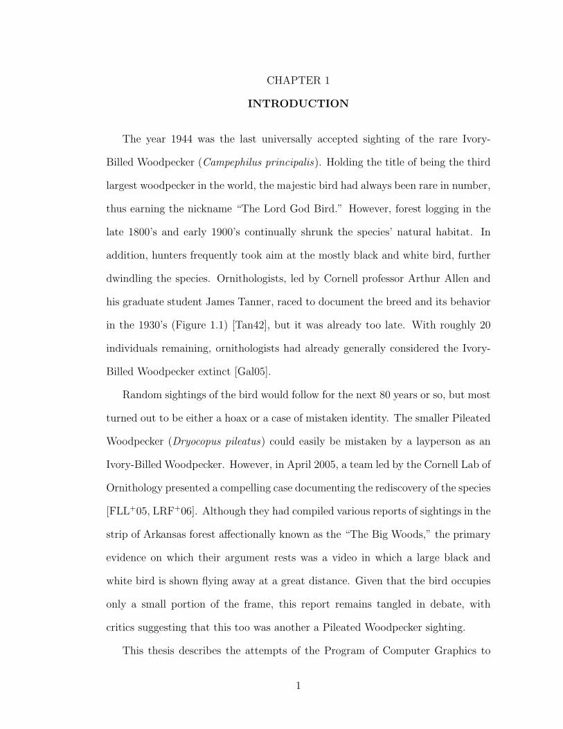
1.1 Still frame of an Ivory-Billed Woodpecker filmed in the late 1930’sby Cornell University ornithologist Arthur Allen [Tan42]. . . . . . . 2

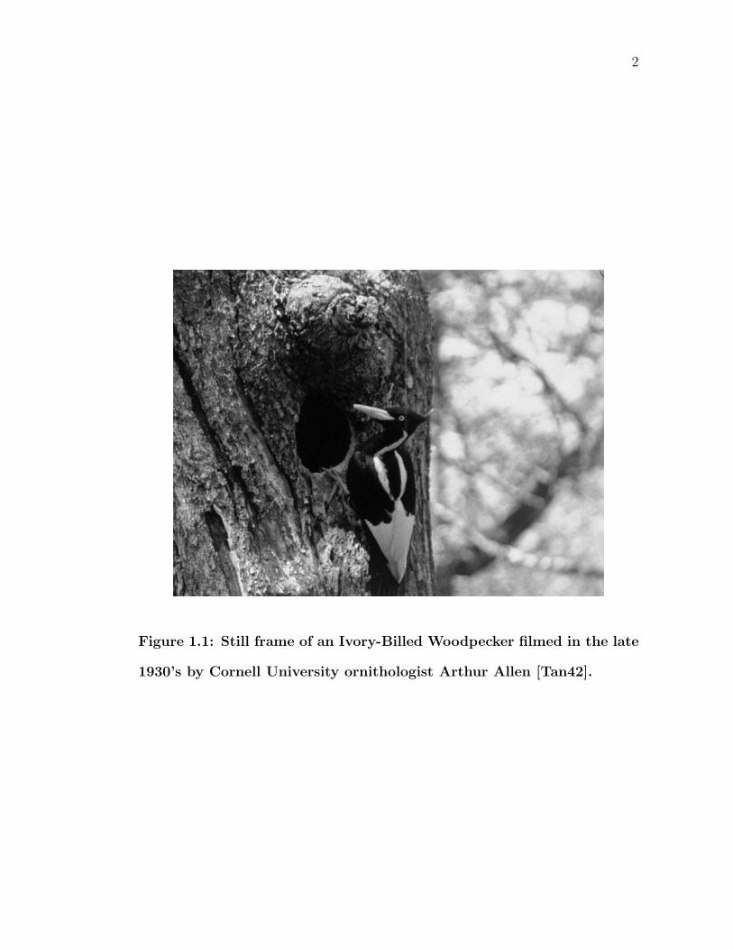
1.2 Key to proving the Ivory-Billed Woodpecker’s rediscovery is inter-preting a fuzzy video of a black and white bird flying away fromthe camera (left, above yellow handle). A deinterlaced still framemagnified by 4x appears above.[FLL+05]. . . . . . . . . . . . . . . 3

2.1 Overall View of a bird [PL93]. . . . . . . . . . . . . . . . . . . . . 82.2 Common anatomic terminology [PRB04]. . . . . . . . . . . . . . . 112.3 Vertebral Column of a Rock Dove [PL93]. . . . . . . . . . . . . . . 142.4 Pectoral Girdle of a Rock Dove [PL93]. . . . . . . . . . . . . . . . . 162.5 Dorsal view of the skeleton from a Rock Dove’s Left Wing [PL93].

The bones of the shoulder girdle are also included for orientationpurposes. . . . . . . . . . . . . . . . . . . . . . . . . . . . . . . . . 16

2.6 Summary of the principal degrees of freedom in an avian wing [Rai85]. 182.7 The pectoralis and supracoracoideus provide the majority of the

force necessary for flight [Bur90]. . . . . . . . . . . . . . . . . . . . 182.8 Automatic hand flexion in a pigeon wing [Vaz94]. Scale bars rep-

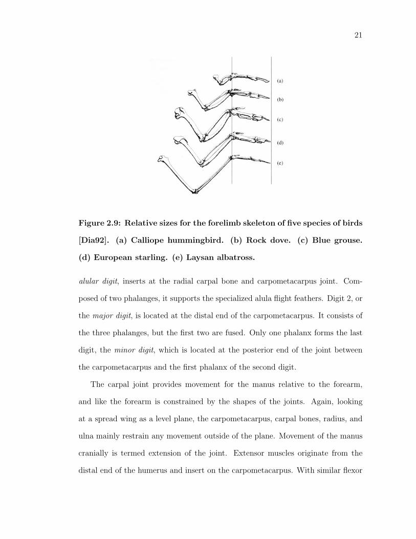
resent 1 cm. . . . . . . . . . . . . . . . . . . . . . . . . . . . . . . . 192.9 Relative sizes for the forelimb skeleton of five species of birds [Dia92].

(a) Calliope hummingbird. (b) Rock dove. (c) Blue grouse. (d) Eu-ropean starling. (e) Laysan albatross. . . . . . . . . . . . . . . . . 21

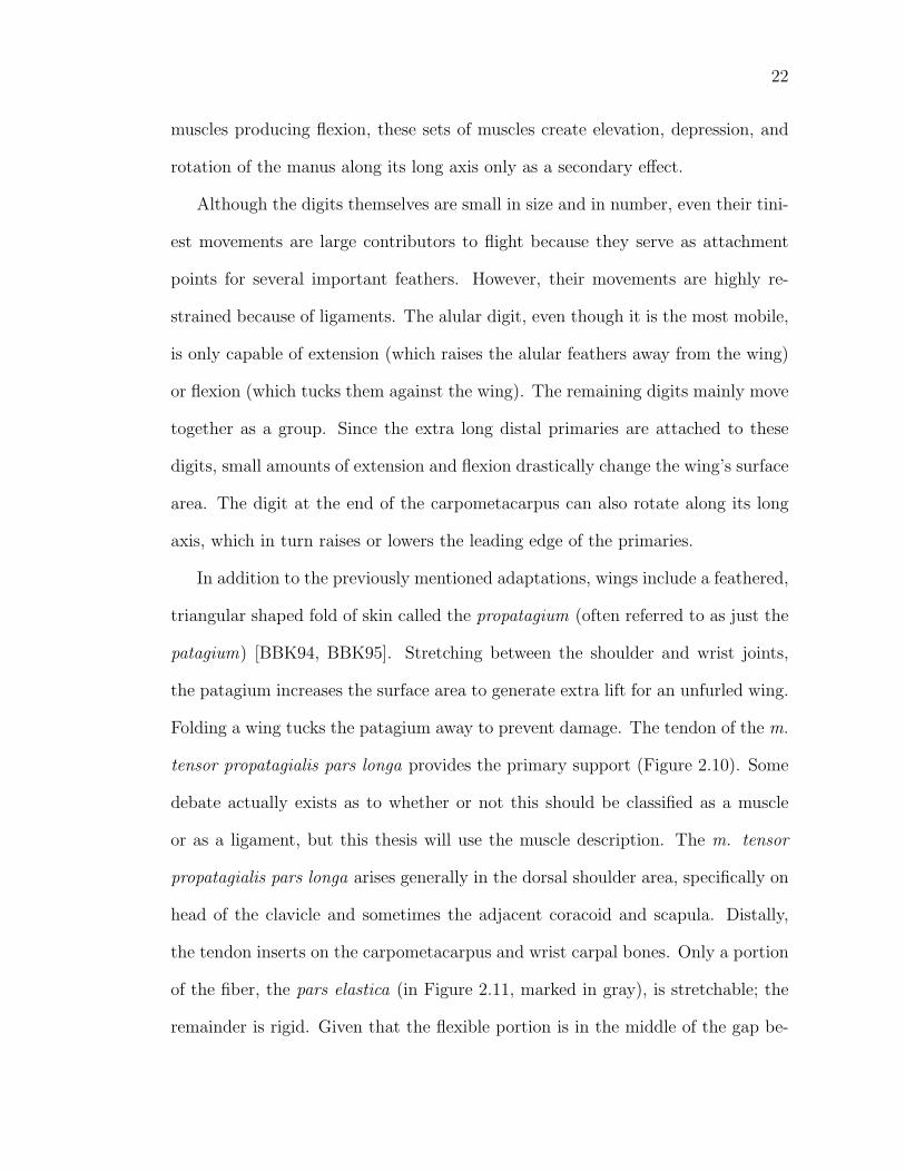
2.10 The m. tensor propatagialis pars longa, the narrow red band run-ning from the shoulder to the wrist, provides the main support forthe patagium [Bur90]. Although relaxed when the wing is folded,wing spreading increases tension in the muscle, helping to keepa straight leading edge when the wing is extended. A secondaryfunction of the patagial muscle aids in automatic wrist extension. . 24

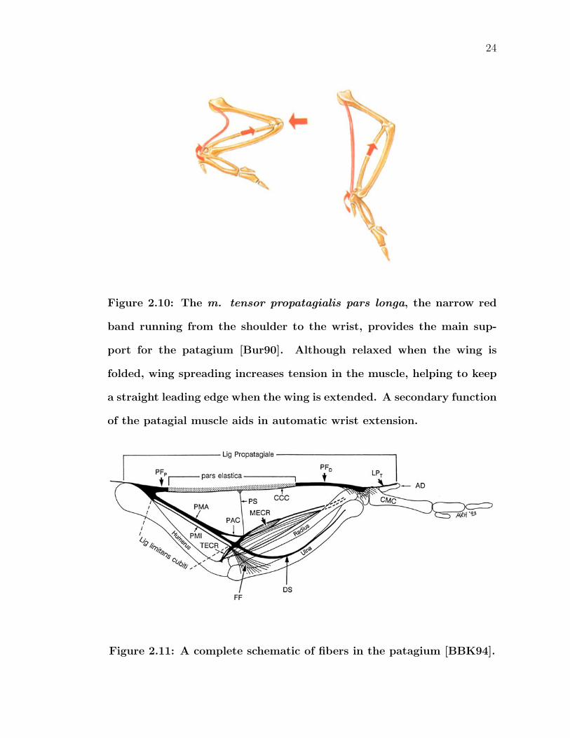
2.11 A complete schematic of fibers in the patagium [BBK94]. . . . . . 242.12 Pelvic Girdle and Right Leg of a Rock Dove [PL93]. . . . . . . . . 252.13 Ivory-Billed Woodpeckers display a rare configuration of the foot

where the three longer digits are pointed relatively forward and thehallux is pointed nearly laterally [BM59]. . . . . . . . . . . . . . . 27

2.14 A Pileated Woodpecker uses his tail to balance himself on the treewhile perching. Adapted from [Soc05]. . . . . . . . . . . . . . . . . 28

2.15 Schematic diagram of the muscles, skeleton, and tail feathers foundin a pigeon. (a) presents a dorsal view, while (b) illustrates a lateralview. [Vid05]. . . . . . . . . . . . . . . . . . . . . . . . . . . . . . . 29

2.16 Structure of a typical contour feather [LS72]. . . . . . . . . . . . . 312.17 Closeup of a feather rachis [LS72]. . . . . . . . . . . . . . . . . . . 32

x

2.18 Scanning electron micrograph of a feather under 110 times magni-fication. The rachis (R), the barbs (B), and the barbules (H) aredisplayed [SH85]. . . . . . . . . . . . . . . . . . . . . . . . . . . . . 33

2.19 With connected barbules, neighboring barbs form an interlockingmatrix [LS72]. . . . . . . . . . . . . . . . . . . . . . . . . . . . . . 34

2.20 Scanning electron micrograph of feather barbules under 2,000 timesmagnification [SH85]. . . . . . . . . . . . . . . . . . . . . . . . . . 35

2.21 Curvature of feathers vanes differ between inner and outer vanes[LS72]. . . . . . . . . . . . . . . . . . . . . . . . . . . . . . . . . . 36

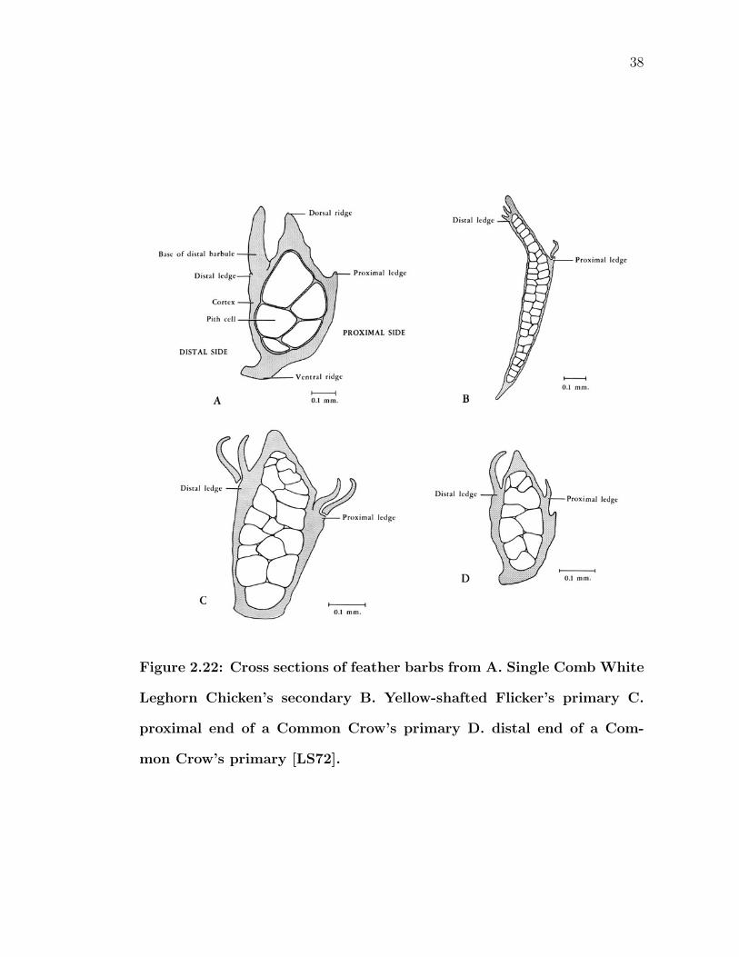
2.22 Cross sections of feather barbs from A. Single Comb White LeghornChicken’s secondary B. Yellow-shafted Flicker’s primary C. proxi-mal end of a Common Crow’s primary D. distal end of a CommonCrow’s primary [LS72]. . . . . . . . . . . . . . . . . . . . . . . . . 38

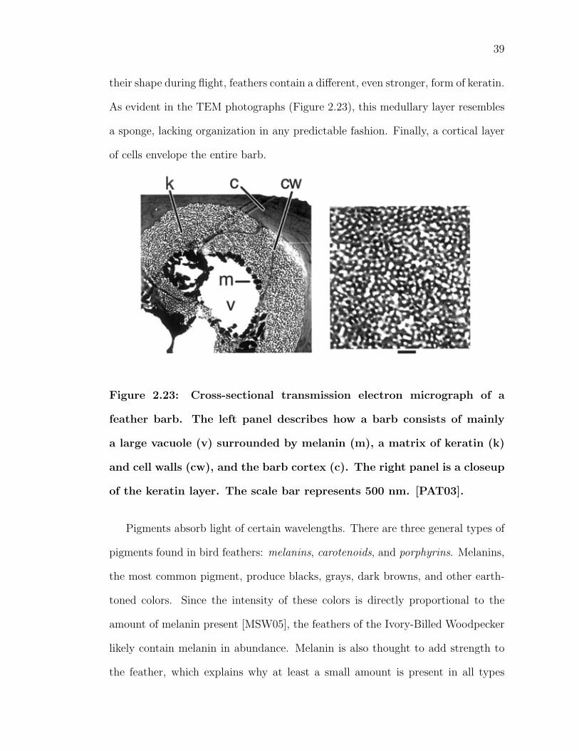
2.23 Cross-sectional transmission electron micrograph of a feather barb.The left panel describes how a barb consists of mainly a large vac-uole (v) surrounded by melanin (m), a matrix of keratin (k) andcell walls (cw), and the barb cortex (c). The right panel is a closeupof the keratin layer. The scale bar represents 500 nm. [PAT03]. . . 39

2.24 Micrograph of a feather displaying a similar glossy-bluish blackcolor that would be found on an Ivory-Billed Woodpecker’s contourfeathers. The bars on the ruler measure 1 mm. . . . . . . . . . . . 41

2.25 Close-up of the barbs from the same feather pictured in the previousfigure. The bars on the ruler measure 1 mm. . . . . . . . . . . . . 42

2.26 Two possible physical mechanisms that explain how light scattersto create structural coloration [PAT03]. . . . . . . . . . . . . . . . 43

2.27 Six feather types are presented here [PL93]. . . . . . . . . . . . . . 452.28 Plumulaceous feathers replace interconnecting barbules with nodal

prongs [LS72]. . . . . . . . . . . . . . . . . . . . . . . . . . . . . . 462.29 A dorsal view of a goshawk wing (top) with cross sections, (a)-(d).

The cross section of primary IX has been enlarged for a closer lookat its shape in (e) [Vid05]. . . . . . . . . . . . . . . . . . . . . . . . 48

2.30 An expanded sagittal cross sectional look at the direction of feathergrowth on the patagium [BBK94]. . . . . . . . . . . . . . . . . . . 49

2.31 Covert feathers covering the wing often come in well defined rows[BBK94]. . . . . . . . . . . . . . . . . . . . . . . . . . . . . . . . . 49

2.32 Still frames of a video, from a dorsal view, depicting wing spreadingon a dead Pilieated Woodpecker. . . . . . . . . . . . . . . . . . . . 51

2.33 Still frames of a video, from a ventral view, depicting wing closingon a dead Pilieated Woodpecker. . . . . . . . . . . . . . . . . . . . 52

2.34 Diagram of the mechanism responsible for spreading flight feathers[Rai85]. . . . . . . . . . . . . . . . . . . . . . . . . . . . . . . . . . 53

2.35 Free Body Diagram of the forces a bird experiences during flight.The forces are assumed to have points of application in roughly thesame planes [Vid05]. . . . . . . . . . . . . . . . . . . . . . . . . . . 55

xi

2.36 An airfoil separates the oncoming air into two separate airstreams[PRB04]. . . . . . . . . . . . . . . . . . . . . . . . . . . . . . . . . 56

2.37 According to Bernoulli’s Principle, the constriction of air above thewing reduces static air pressure [Bur90]. . . . . . . . . . . . . . . . 57

2.38 Neither of these conditions generate lift. No air moves over thewing in the left diagram, and an incorrect airfoil shape (right) failsto create pressure differences [PRB04]. . . . . . . . . . . . . . . . . 57

2.39 Effect of angle of attack on lift and turbulence [PRB04]. . . . . . . 592.40 Under slow speed flying conditions, alular feathers act like a slat to

maintain a smooth airflow [Bur90]. . . . . . . . . . . . . . . . . . . 602.41 Photograph of a bird extending its alula [Bur90]. . . . . . . . . . . 612.42 Dial91 recorded wing joint rotation angles during a wingbeat [DGJ91].

The top three figures show a starling through three different views:anteriorally, sagitally, and posteriorally. The letters label six differ-ent points of a wingbeat: (A) upstroke-downstroke transition, (B)early downstroke, (C) mid downstroke, (D) downstroke-upstroketransition, (E) early upstroke, and (F) late upstroke. . . . . . . . . 64

2.43 The furcula acts like a spring during a wingbeat [JJDGJ88]. . . . . 652.44 The muscles used during a wingbeat causes movements in the joints

of the pectoral girdle [JJDGJ88]. . . . . . . . . . . . . . . . . . . . 662.45 Marey made bronze statues of one wingbeat cycle to show that

birds sweep their wings downward and forward during downstroke[Mar90]. . . . . . . . . . . . . . . . . . . . . . . . . . . . . . . . . . 67

2.46 The force (K) acting on a wing as a result of the oncoming air-flow can be separated into a vertical component, lift (L), and alsothrust (T). Without feather rotation, only a small amount of for-ward thrust is generated [Ten96]. . . . . . . . . . . . . . . . . . . . 69

2.47 Rotating the primary feathers reduces the angle of attack and in-creases the horizontal component of the resulting force, creatingadditional thrust [PRB04]. . . . . . . . . . . . . . . . . . . . . . . 69

2.48 Relative strain measurements taken on the 9th primary feather(top). A single wingbeat is expanded (below) for clarity [CB98]. . . 72

2.49 Lateral views of steady-velocity flight illustrating the path of awingbeat for a range of speeds in a domestic pigeon [TD96]. . . . . 73

3.1 Key curves (left) are linearly interpolated in [SH02] to create thefinal feather (right). . . . . . . . . . . . . . . . . . . . . . . . . . . 76

3.2 Chen et al. [CXGS02] added controls to define the outer boundaryof a feather (dotted lines). . . . . . . . . . . . . . . . . . . . . . . . 77

3.3 A progressively closer look at Chen et al’s [CXGS02] results showthat it is difficult with their algorithm to model feathers that haveshapes different from non-flight feathers. . . . . . . . . . . . . . . . 79

xii

3.4 Instead of modeling several different types of feathers, Sony Image-works used a fur simulation in many areas, particularly near thehead and torso areas. . . . . . . . . . . . . . . . . . . . . . . . . . 80

3.5 Rendering with a BTF (right) yielded small visual details not foundin the non-BTF version (left) [CXGS02]. . . . . . . . . . . . . . . . 82

3.6 Realistic rendering of hair or feather requires scattering calcula-tions. [MJC+03]’s scattering model variation of color and bright-ness of hair fiber due to changes in lighting direction. . . . . . . . . 83

3.7 The final fur/feather curve was interpolated from key curves [Bru03]. 863.8 A water simulation used constraints set on the last frame of the

animation to solve for the forces necessary to generate the shapes(a cross, torus, and man) [MTPS04]. . . . . . . . . . . . . . . . . . 89

3.9 Ramakrishnananda and Wong [RW99] incorporate a simple, boxymodel of a bird that lacks the appropriate degrees of freedom whensimuating the aerodynamics. . . . . . . . . . . . . . . . . . . . . . 91

3.10 The degrees of freedom (DOFs) for the bird model used by Wu andPopovic closely match those of a real bird. . . . . . . . . . . . . . . 92

4.1 Typical values for radiographic density, measured in Housefieldunits (HU), are summarized in the graph [FB04]. . . . . . . . . . . 97

4.2 In modern day CT scanners, the patient lies on a table at the centerof a rotating gantry which holds an x-ray emitter. Also surroundingthe patient is a ring of detectors that measure x-ray transmittance[FB04]. . . . . . . . . . . . . . . . . . . . . . . . . . . . . . . . . . 98

4.3 Two different images of the same lung cross section, but with dif-ferent windowing parameters, are presented. Structures visible inone image are not visible in the other [FB04]. . . . . . . . . . . . . 99

4.4 After measured attenuation values for an object are mapped ona histogram, window width and window level parameters can beadjusted to include only the materials of interest (adapted from[CKH+99]). . . . . . . . . . . . . . . . . . . . . . . . . . . . . . . . 100

4.5 Pickled Ivory-Billed Woodpecker specimen. . . . . . . . . . . . . . 1014.6 In this example slice, the contours used for reconstruction (yellow)

have been automatically generated through thresholding, but erro-neously contain feathers in addition to the skin. This is particularlyevident in the wing (top right inset). . . . . . . . . . . . . . . . . . 105

4.7 Contours have been manually modified to remove the feathers, leav-ing just the skin. . . . . . . . . . . . . . . . . . . . . . . . . . . . . 107

4.8 Surface reconstruction from contours generally consist of four sub-problems, three of which are pictured above - the correspondenceproblem, the tiling problem, and the branching problem. The final,surface fitting problem, smooths the resulting mesh [MSS92]. . . . 108

4.9 Rendered image of the Ivory-Billed Woodpecker’s skin recoveredfrom the CT scan data, in a tucked wing pose. . . . . . . . . . . . 111

xiii

4.10 Rendered image of the reconstructed Ivory-Billed Woodpecker’sskeletal surface, in the same tucked wing pose as the previous figure.Image courtesy of DigiMorph. . . . . . . . . . . . . . . . . . . . . . 112

4.11 Comparison between the original reconstructed model (dark gray)and smoothed animation model (wireframe). . . . . . . . . . . . . . 116

4.12 Comparison between the original reconstructed model (dark gray)and smoothed animation model (wireframe). . . . . . . . . . . . . . 117

4.13 The polygon smoothing operation is approximating, introducingvolume differences between the resulting smooth model (red) andthe original base model (gray). . . . . . . . . . . . . . . . . . . . . 118

4.14 Photographs of stuffed specimens (left column) and renderings ofour revised model (right column). . . . . . . . . . . . . . . . . . . . 119

4.15 A sketch of the Ivory-Billed’s feet presented in [BM59], at left. Ourmodeled feet for comparison is shown at right. . . . . . . . . . . . . 120

5.1 Smooth skinning algorithm on an elbow joint . . . . . . . . . . . . 1245.2 Dorsal view (top) and postlateral view (bottom) of the animation

joints (black spheres) and the recovered CT scan data (light gray). 1255.3 Closeup of the joints in the forearm. . . . . . . . . . . . . . . . . . 1265.4 Dorsal view of forearm rotation. . . . . . . . . . . . . . . . . . . . 1275.5 Anterior view of the shoulder girdle. The recovered CT geometry

appears in light gray, while the animation joints appear as darkspheres. . . . . . . . . . . . . . . . . . . . . . . . . . . . . . . . . . 128

5.6 The patagium in our animated model is deformed by joints thatmimic the actual tendon. . . . . . . . . . . . . . . . . . . . . . . . 130

5.7 Comparison of our patagial model versus one seen on a real speci-men, with the wing in an open (top) and a closed position (bottom).132

5.8 Neck skeleton and rig. . . . . . . . . . . . . . . . . . . . . . . . . . 1335.9 Leg skeleton and rig. . . . . . . . . . . . . . . . . . . . . . . . . . . 135

6.1 Feather construction operations typically occur in a local spacedefined at the root joint, one of which is shown in the top picture.Two other joints help define a feather, as seen in the fully featheredright wing (below). . . . . . . . . . . . . . . . . . . . . . . . . . . . 141

6.2 Extrusion of a deformed circle to form the rachis geometry, withdots representing control vertices. . . . . . . . . . . . . . . . . . . . 143

6.3 Vane modeling starts with a loft operation to form a flat NURBSsurface. . . . . . . . . . . . . . . . . . . . . . . . . . . . . . . . . . 145

6.4 A smooth step function returns a value between zero and one whenfed a value, x, that lie between boundaries a and b. . . . . . . . . . 147

6.5 Looking down the axis of the rachis, the feather model captures thevertical, concave curvature seen in real feathers. . . . . . . . . . . . 148

xiv

6.6 Macroscale geometry of an example feather. The visible portion isshown in dark gray, and, for explanation purposes only, the partswhich are trimmed away are displayed in light gray. . . . . . . . . . 149

6.7 The appearance of complex surfaces (top) can be quickly simulatedusing bump mapping by perturbing the normal vectors of less com-plex (and less tessellated) surfaces. . . . . . . . . . . . . . . . . . . 150

6.8 A rendered feather with bump maps to create barbs. A selectedportion, isolated with white, is displayed in a closeup (below) tobetter reveal details. . . . . . . . . . . . . . . . . . . . . . . . . . . 151

6.9 The appearance of complex surfaces (top) can be quickly simulatedusing bump mapping by perturbing the normal vectors of less com-plex (and less tessellated) surfaces. Control vertices are representedby dots. . . . . . . . . . . . . . . . . . . . . . . . . . . . . . . . . . 152

6.10 Our manually-created model of the Pileated spread wing (yellow)closely matches the geometry acquired by the laser range scan (lightgray). . . . . . . . . . . . . . . . . . . . . . . . . . . . . . . . . . . 154

6.11 The modeled Pileated spread wing was used as alignment referencefor the animated Ivory-Billed feathers. . . . . . . . . . . . . . . . . 155

6.12 Rotation angles are calculated for the feather root joints as a weightedaverage of the orthonormal bases located at the elbow and thewingtip (both are shown in white). . . . . . . . . . . . . . . . . . . 158

6.13 An adjustable polynomal provides the weights for the wing tip lo-cator, when setting orientation constraints on the feathers. Thecolors represent to what the degree the function is raised: black =linear, dark blue = cubic, orange = 5th power. . . . . . . . . . . . 159

6.14 Rotation of the twist joints simulate the deformation in primaryfeathers that occur as a result of their interaction with aerodynamicforces. . . . . . . . . . . . . . . . . . . . . . . . . . . . . . . . . . . 161

6.15 The tail can be either closed (top) or spread (bottom). . . . . . . . 1636.16 The tight band of green in the hemispherical plot of reflectance (top

right) corroborates our previous claims that feathers scatter lightin a directionally dependent manner. . . . . . . . . . . . . . . . . . 164

6.17 The white feathers on this stuffed specimen of an Ivory-Billed Wood-pecker are not solidly white, but contain a mixture of subtle detailswhich reflect signs of age, dirt, and wear. . . . . . . . . . . . . . . 166

6.18 Diffuse color map for a feather. . . . . . . . . . . . . . . . . . . . . 1676.19 Rendering of the left wing feathers on our Ivory-Billed Woodpecker

model. . . . . . . . . . . . . . . . . . . . . . . . . . . . . . . . . . . 1676.20 An example of a transparency map used to reproduce the breaks in

the vane that result from barbs no longer being connected by theirbarbules. . . . . . . . . . . . . . . . . . . . . . . . . . . . . . . . . 168

6.21 Adaptive sampling in the Maya Renderer [BGH+04]. . . . . . . . . 171

xv

6.22 A low tessellation render of a feather appears at top, followed by ahighly tessellated version. The difference image between these tworenderings is shown at the bottom, where large differences in twocorresponding pixels appear as brighter intensities. . . . . . . . . . 173

6.23 Rendered image of Ivory-Billed Woodpecker with fur to approxi-mate torso feathers. . . . . . . . . . . . . . . . . . . . . . . . . . . 175

6.24 Closeup of fur simulation to approximate torso feathers. . . . . . . 1766.25 Attributes for the fur simulation are specified by texture maps. The

map shown above specifies the length of fur. . . . . . . . . . . . . . 1776.26 The importance of self-shadowing to a realistic rendering is demon-

strated above. The image at left is rendered with self-shadowing,whereas the right one is not [LV00]. . . . . . . . . . . . . . . . . . 178

xvi

CHAPTER 1

INTRODUCTION

The year 1944 was the last universally accepted sighting of the rare Ivory-

Billed Woodpecker (Campephilus principalis). Holding the title of being the third

largest woodpecker in the world, the majestic bird had always been rare in number,

thus earning the nickname “The Lord God Bird.” However, forest logging in the

late 1800’s and early 1900’s continually shrunk the species’ natural habitat. In

addition, hunters frequently took aim at the mostly black and white bird, further

dwindling the species. Ornithologists, led by Cornell professor Arthur Allen and

his graduate student James Tanner, raced to document the breed and its behavior

in the 1930’s (Figure 1.1) [Tan42], but it was already too late. With roughly 20

individuals remaining, ornithologists had already generally considered the Ivory-

Billed Woodpecker extinct [Gal05].

Random sightings of the bird would follow for the next 80 years or so, but most

turned out to be either a hoax or a case of mistaken identity. The smaller Pileated

Woodpecker (Dryocopus pileatus) could easily be mistaken by a layperson as an

Ivory-Billed Woodpecker. However, in April 2005, a team led by the Cornell Lab of

Ornithology presented a compelling case documenting the rediscovery of the species

[FLL+05, LRF+06]. Although they had compiled various reports of sightings in the

strip of Arkansas forest affectionally known as the “The Big Woods,” the primary

evidence on which their argument rests was a video in which a large black and

white bird is shown flying away at a great distance. Given that the bird occupies

only a small portion of the frame, this report remains tangled in debate, with

critics suggesting that this too was another a Pileated Woodpecker sighting.

This thesis describes the attempts of the Program of Computer Graphics to

1

2

Figure 1.1: Still frame of an Ivory-Billed Woodpecker filmed in the late

1930’s by Cornell University ornithologist Arthur Allen [Tan42].

3

collaborate with the Lab of Ornithology in their quest to verify the existence of

the Ivory-Billed Woodpecker.

Figure 1.2: Key to proving the Ivory-Billed Woodpecker’s rediscovery is

interpreting a fuzzy video of a black and white bird flying away from the

camera (left, above yellow handle). A deinterlaced still frame magnified

by 4x appears above.[FLL+05].

When we first contacted the Cornell Lab of Ornithology about their finding,

our original intention was to help scientifically determine what species of bird

appears in the video. Since the wings of the Pileated and Ivory-Billed Woodpeckers

have nearly opposite coloring, interpreting the wings’ orientation in relation to the

camera during the wingbeats captured on video lies at the center of this argument.

By constructing an animated Ivory-Billed Woodpecker and an animated Pileated

Woodpecker, complete with their respective coloration and flying styles, we hoped

to pattern match our animation with the video. However, in trying to make a

realistic animation of a flying bird, we found many challenges when attempting to

make it physically and physiologically correct and thus shifted our focus in this

direction.

The ubiquitous video games, animated movies, and special effects are indicators

4

of how far computer graphics research has evolved. Techniques developed in the

last ten years or more have certainly tricked our eyes into believing that what

we’re seeing is real. However, important distinctions still remain, between what

is believable and what is actually real. Furthermore, the computer graphics world

has yet to mature its collaboration with the scientific community as much as it has

with the entertainment industry. Algorithms have become increasingly artistically

driven, concentrating on generating exquisite digital images and videos, but often

sacrificing physical accuracy. Most commonly used algorithms and procedures have

inherent shortcomings, and can not be used for physical simulations.

Physically-based lighting stands out as a major exception to this trend. Ra-

diosity, path tracing, and, most recently, photon mapping provide methods to solve

the rendering equation which result in images that are not longer just believable

but physically accurate as well [CG85, Kaj86, JC98].

The same treatment should be employed on the other sectors of the realism

puzzle: shape and motion. Decreasing costs of memory now allow for geomet-

ric models of increased complexity, while subdivision and parametric surfaces are

useful to compactly represent these structures [DKT98, PT97]. At the same time,

modalities for obtaining a precise measurement of an object’s form, including those

visible and invisible to the eye, now exist. Laser-range scanners have made it pos-

sible to capture shape with millimeter accuracy. Computerized tomography (CT)

machines can image below the skin surface and acquire the geometry of internal or-

gans with sub-millimeter precision. The publicly available Visible Human Dataset

[SASW96, SW98], featuring a complete scan of both the male and female body,

symbolizes the robustness of such technology.

Motion and dynamic behavior are topics still in their infancy. Recent research

5

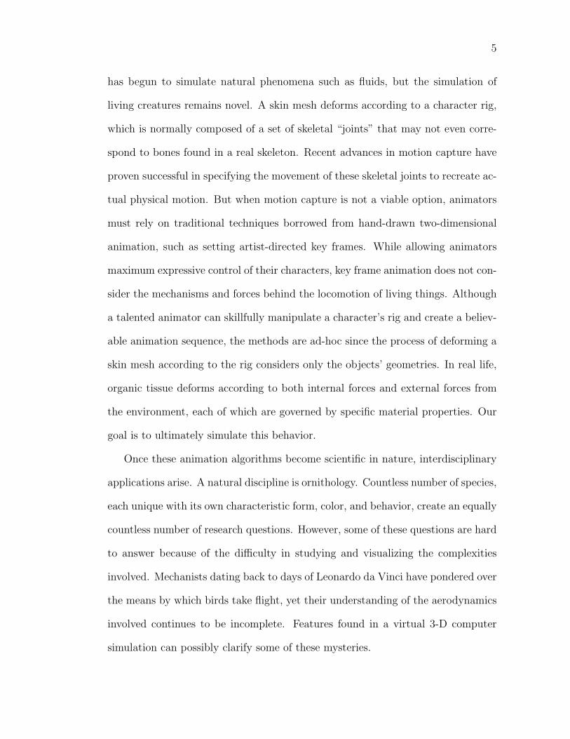
has begun to simulate natural phenomena such as fluids, but the simulation of

living creatures remains novel. A skin mesh deforms according to a character rig,

which is normally composed of a set of skeletal “joints” that may not even corre-

spond to bones found in a real skeleton. Recent advances in motion capture have

proven successful in specifying the movement of these skeletal joints to recreate ac-

tual physical motion. But when motion capture is not a viable option, animators

must rely on traditional techniques borrowed from hand-drawn two-dimensional

animation, such as setting artist-directed key frames. While allowing animators

maximum expressive control of their characters, key frame animation does not con-

sider the mechanisms and forces behind the locomotion of living things. Although

a talented animator can skillfully manipulate a character’s rig and create a believ-

able animation sequence, the methods are ad-hoc since the process of deforming a

skin mesh according to the rig considers only the objects’ geometries. In real life,

organic tissue deforms according to both internal forces and external forces from

the environment, each of which are governed by specific material properties. Our

goal is to ultimately simulate this behavior.

Once these animation algorithms become scientific in nature, interdisciplinary

applications arise. A natural discipline is ornithology. Countless number of species,

each unique with its own characteristic form, color, and behavior, create an equally

countless number of research questions. However, some of these questions are hard

to answer because of the difficulty in studying and visualizing the complexities

involved. Mechanists dating back to days of Leonardo da Vinci have pondered over

the means by which birds take flight, yet their understanding of the aerodynamics

involved continues to be incomplete. Features found in a virtual 3-D computer

simulation can possibly clarify some of these mysteries.

6

To transform an animation of bird flight into a simulation, both the physical

and phsyiological mechanisms that govern shape and motion need to be precisely

modeled. The animation of the Ivory-Billed Woodpecker described in this thesis

represents the foundation for this research. To obtain accurate geometric data, a

preserved Ivory-Billed Woodpecker specimen, with its internal organs and skeleton

intact, was CT scanned. The resulting slices of volumetric data were reconstructed

to provide two separate three dimensional models: one of the skeleton and another

of the bird’s skin. These two models afforded us with precise measurements and

proportions, which were then used as reference to create the geometric model and

skeleton for our animation. With user specification to define the shape and orien-

tation, a procedural system modeled and animated the flight feathers on the Ivory-

Billed’s wings. Feathers on the torso were approximated with standard graphics

fur simulation algorithms. Joints in our character rig were animated using data

adapted from previously published ornithological research on the kinematics of

bird flight.

The remainder of the thesis, subdivided into five chapters, provides a detailed

exploration of the tasks required to accurately animate bird flight. Chapter 2

acquaints readers with the necessary background knowledge on avian morphology

for this thesis and for future work. Chapter 3 reviews published work related to

birds and bird flight in computer graphics. Chapter 4 explains the reconstruction

of the Ivory-Billed from the CT scan. Chapter 5 details the feathering of our

model. Chapter 6 examines how our model was animated. Finally, conclusions

and future work are presented in Chapter 7.

CHAPTER 2

AVIAN MORPHOLOGY

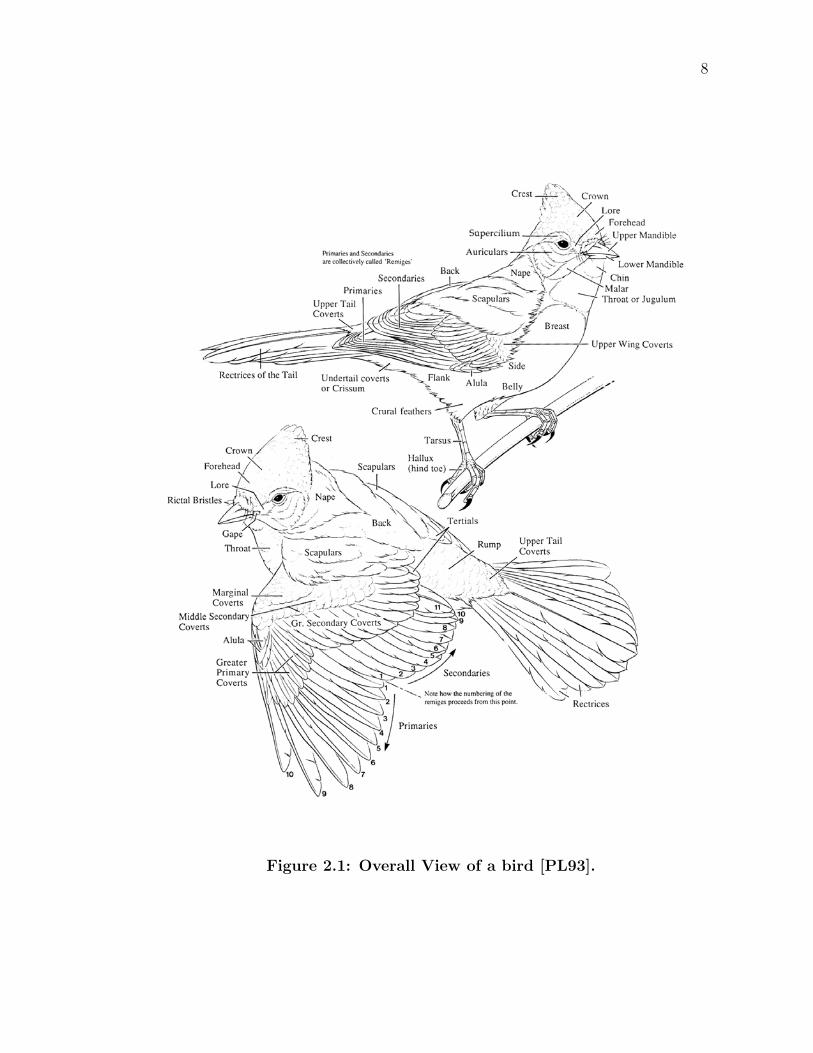
After taking a quick “gander” at any bird (Figure 2.1), it’s hard to believe

that they originally evolved from reptiles. However, some 150 to 200 million years

after their divergence from their ancestors, birds possess specialized adaptations for

flying. While the result is a light, efficient flying machine, the question, “How does

a bird fly?” is still difficult to answer. Since this thesis provides the foundation

for faithfully reproducing an accurate model of bird flight, a good understanding

of the form, characteristics, and functions of bird anatomy becomes important to

answering this question.

2.1 General Characteristics

2.1.1 Feathers

The most obvious indicator of a bird are its feathers. As a large part of the

integumentary system, feathers provide protection from parasites/disease/damage,

insulation, and species/gender identification.

Several different types of feathers exist on any single bird. Of particular interest

in this thesis are the feathers attached to the posterior edges of the wings and tail,

the remiges and rectrices, respectively. They are the main aerodynamic surfaces

that allow the bird to fly; thus, as a group, they are appropriately named flight

feathers. Remiges are further broken down into primaries and secondaries accord-

ing to their location on the wing. In turn, the remiges are generally overlapped at

the base by a series of covert feathers.

7

8

Figure 2.1: Overall View of a bird [PL93].

9

2.1.2 Bill

The upper and lower mandibles form the bird’s bill. This too is an evolutionary

adaptation for flying. Birds lack teeth, shedding the weight of teeth and the jaw

bones needed to support them.

2.1.3 Strong Skeleton

The avian skeleton, while similar in some regards to other vertebrates, are often

more specialized than their counterparts. For example, mammals typically have

solid bones. However, the major bones in a bird are pneumatized, meaning they

are hollow and contain air sacs that connect directly to the respiratory system.

Bones of this type are extremely strong relative to other regular bones of the same

mass. Interestingly enough, although the bone is lighter, the actual material often

tends to have identical or greater densities than their counterparts. Additionally,

the skeleton is also able to provide significant support because components are

often fused together. Other places showing extensive fusion include the head and

spine.

2.1.4 Bipedal feet

During flight, birds hide much of their drag-inducing legs underneath the sleek

exterior of their feathers, obviously for aerodynamic purposes. The joint analogous

to the human knee is not visible.

10

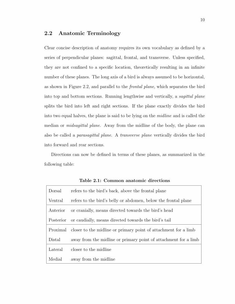
2.2 Anatomic Terminology

Clear concise description of anatomy requires its own vocabulary as defined by a

series of perpendicular planes: sagittal, frontal, and transverse. Unless specified,

they are not confined to a specific location, theoretically resulting in an infinite

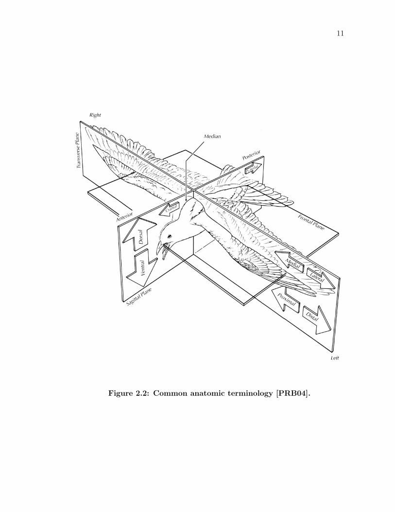
number of these planes. The long axis of a bird is always assumed to be horizontal,

as shown in Figure 2.2, and parallel to the frontal plane, which separates the bird

into top and bottom sections. Running lengthwise and vertically, a sagittal plane

splits the bird into left and right sections. If the plane exactly divides the bird

into two equal halves, the plane is said to be lying on the midline and is called the

median or midsagittal plane. Away from the midline of the body, the plane can

also be called a parasagittal plane. A transverse plane vertically divides the bird

into forward and rear sections.

Directions can now be defined in terms of these planes, as summarized in the

following table:

Table 2.1: Common anatomic directions

Dorsal refers to the bird’s back, above the frontal plane

Ventral refers to the bird’s belly or abdomen, below the frontal plane

Anterior or cranially, means directed towards the bird’s head

Posterior or caudially, means directed towards the bird’s tail

Proximal closer to the midline or primary point of attachment for a limb

Distal away from the midline or primary point of attachment for a limb

Lateral closer to the midline

Medial away from the midline

11

Figure 2.2: Common anatomic terminology [PRB04].

12

2.3 Musculoskeletal System

The musculoskeletal system of a bird comprises the majority of its mass and con-

sists of bone, muscle, and ligaments.

Muscles produce contractile force resulting in motion. Although many mus-

cles fall into the category of involuntary muscle, producing contraction without

conscious thought or direction, the muscles presented here are of the skeletal or

voluntary muscle variety. Tendons anchor these types of muscles to at least two or

more bones. The proximal attachment point is referred to as the origin, as opposed

to insertion for the distal end. Birds do not have a uniform distribution of muscle

and concentrate their mass primarily ventrally, below the wings and the center of

the gravity.

Ligaments are connective tissue that provide mechanical stability in joints.

Made out of elastic collagen fibers, they will lengthen when subjected to tensile

force, but only to a certain extent. Thus, ligaments restrict the mobility of joints,

sometimes completely preventing certain movements.

An exhaustive listing of ligaments and muscles is beyond the scope of this

thesis. Wings alone contain some 45 muscles. The primary ones responsible for

flight are discussed later.

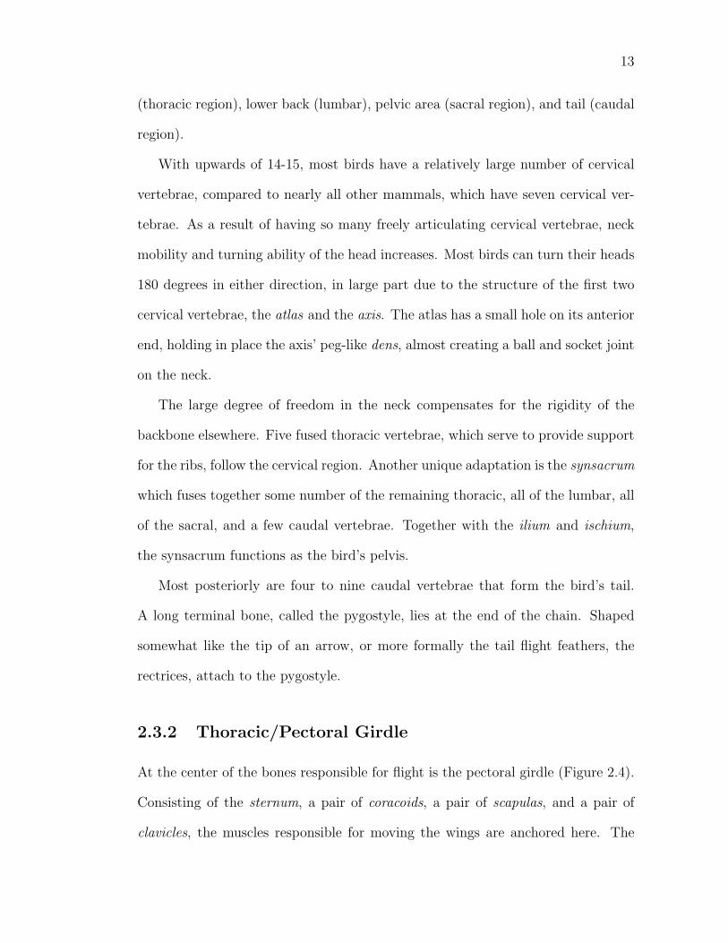
2.3.1 Vertebral Column

Bones which support the spinal cord are called vertebrae, and together they form

the vertebral column or more commonly, the “backbone” (Figure 2.3). They are

then grouped by their general position along the length of the spine and num-

bered within each region. Five groupings exist: the neck (cervical region), thorax

13

(thoracic region), lower back (lumbar), pelvic area (sacral region), and tail (caudal

region).

With upwards of 14-15, most birds have a relatively large number of cervical

vertebrae, compared to nearly all other mammals, which have seven cervical ver-

tebrae. As a result of having so many freely articulating cervical vertebrae, neck

mobility and turning ability of the head increases. Most birds can turn their heads

180 degrees in either direction, in large part due to the structure of the first two

cervical vertebrae, the atlas and the axis. The atlas has a small hole on its anterior

end, holding in place the axis’ peg-like dens, almost creating a ball and socket joint

on the neck.

The large degree of freedom in the neck compensates for the rigidity of the

backbone elsewhere. Five fused thoracic vertebrae, which serve to provide support

for the ribs, follow the cervical region. Another unique adaptation is the synsacrum

which fuses together some number of the remaining thoracic, all of the lumbar, all

of the sacral, and a few caudal vertebrae. Together with the ilium and ischium,

the synsacrum functions as the bird’s pelvis.

Most posteriorly are four to nine caudal vertebrae that form the bird’s tail.

A long terminal bone, called the pygostyle, lies at the end of the chain. Shaped

somewhat like the tip of an arrow, or more formally the tail flight feathers, the

rectrices, attach to the pygostyle.

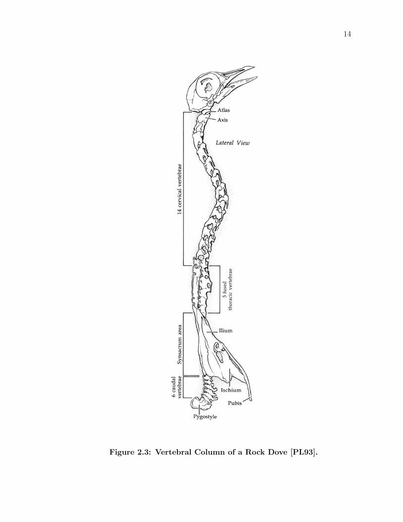
2.3.2 Thoracic/Pectoral Girdle

At the center of the bones responsible for flight is the pectoral girdle (Figure 2.4).

Consisting of the sternum, a pair of coracoids, a pair of scapulas, and a pair of

clavicles, the muscles responsible for moving the wings are anchored here. The

14

Figure 2.3: Vertebral Column of a Rock Dove [PL93].

15

sternum is the centerpiece of the system and two principal flight muscles, the m.

pectoralis and m. supracoracoideus, originate mainly from the keel of the sternum.

Birds that are unable to fly possess sternums which are reduced in size and are

missing a keel. The sternum is linked to the rest of the girdle by post-like structures

called coracoids. These coracoids run craniodorsolaterally. Further stabilizing the

unit are the clavicles. Unlike humans, the two clavicles are actually fused together

to form the furcula, or what is popularly known as the “wishbone.” Completing

the girdle are the two scapulas - long bones that run in a general anterior/posterior

direction. The glenoid cavity (or glenoid fossa) is located at the lateral side of the

clavicle and coracoid joint. At the posterior end of each scapula is a flat, blade-like

ending extending caudually over the rib cage. Together, these three bones of the

pectoral girdle join at a point called the trioseal canal. The dorsal head of the

coracoid has two projections that form a U-shape cavity. The anterior end of the

scapula caps the hole, completing a tunnel through which the tendon of the m.

supracoracoideus passes.

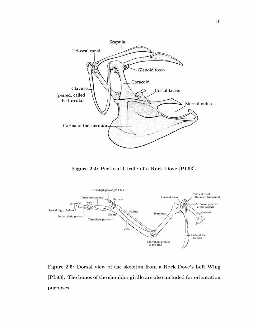
2.3.3 Wings

Wings are laid out much like the arms of a human or other vertebrates. It consists

of the humerus (upper arm bone), radius and ulna (forearm bones), carpal (wrist)

bones, and a series of digits or fingers making up the manus (hand) (Figure 2.5).

Humerus bones are typically thick, strong and short. This is because the pri-

mary flight muscles of the chest area only have points of insertion on the humerus.

Longer humerus bones would require more work done by the flight muscles to gen-

erate the torque needed to flap the wings. The humerus/pectoral girdle joint is

much like any ball-socket joint, except the ball end more closely resembles an egg.

16

Figure 2.4: Pectoral Girdle of a Rock Dove [PL93].

Figure 2.5: Dorsal view of the skeleton from a Rock Dove’s Left Wing

[PL93]. The bones of the shoulder girdle are also included for orientation

purposes.

17

The ball portion of the joint contains the pectoral crest, or where the m. pectoralis

inserts. The socket half of the shoulder joint is the glenoid fossa.

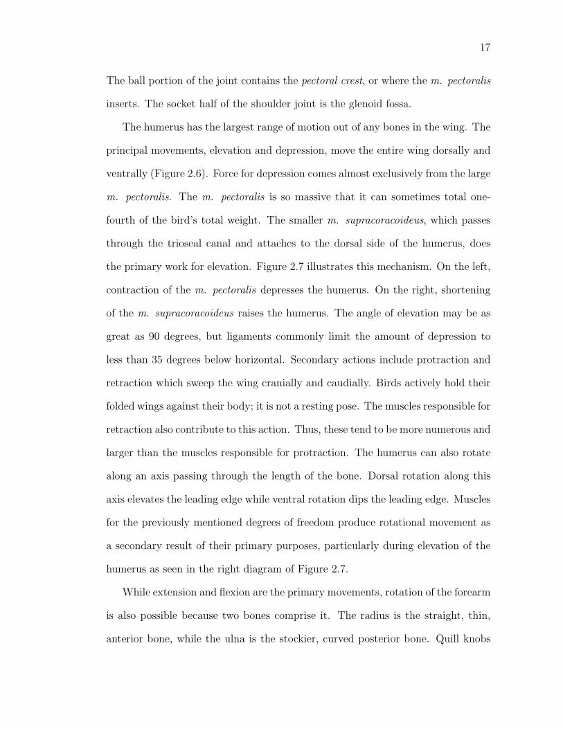
The humerus has the largest range of motion out of any bones in the wing. The

principal movements, elevation and depression, move the entire wing dorsally and

ventrally (Figure 2.6). Force for depression comes almost exclusively from the large

m. pectoralis. The m. pectoralis is so massive that it can sometimes total one-

fourth of the bird’s total weight. The smaller m. supracoracoideus, which passes

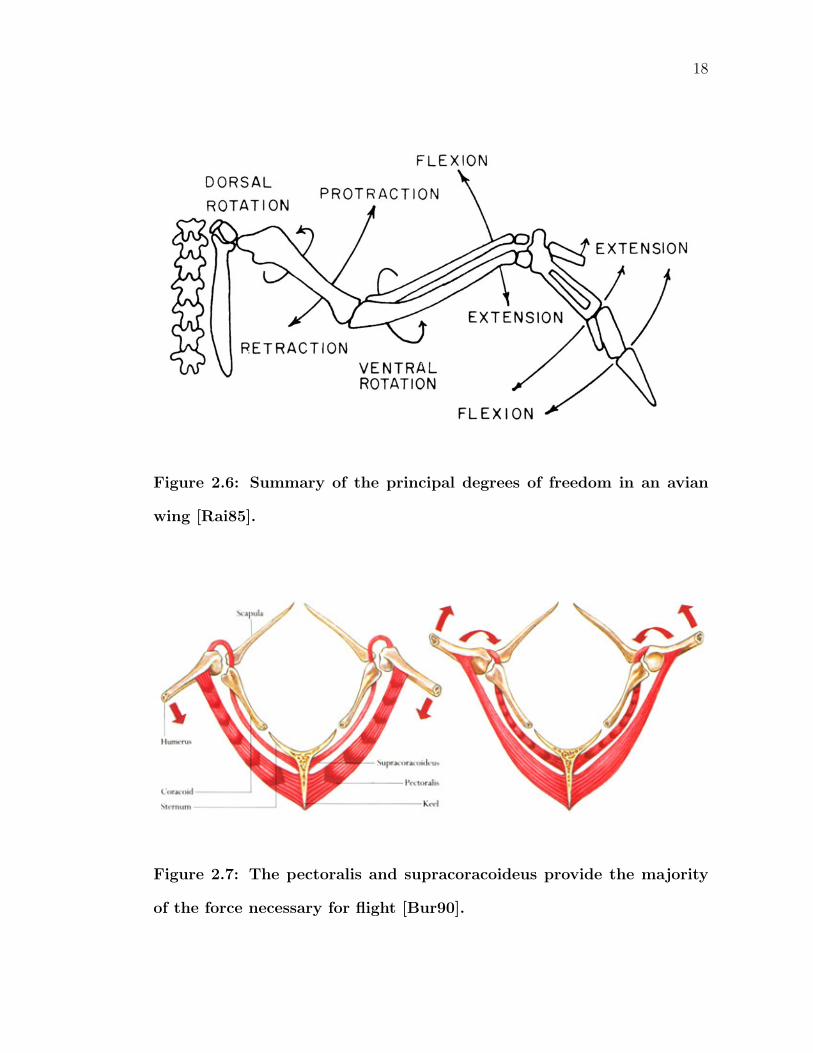
through the trioseal canal and attaches to the dorsal side of the humerus, does

the primary work for elevation. Figure 2.7 illustrates this mechanism. On the left,

contraction of the m. pectoralis depresses the humerus. On the right, shortening

of the m. supracoracoideus raises the humerus. The angle of elevation may be as

great as 90 degrees, but ligaments commonly limit the amount of depression to

less than 35 degrees below horizontal. Secondary actions include protraction and

retraction which sweep the wing cranially and caudially. Birds actively hold their

folded wings against their body; it is not a resting pose. The muscles responsible for

retraction also contribute to this action. Thus, these tend to be more numerous and

larger than the muscles responsible for protraction. The humerus can also rotate

along an axis passing through the length of the bone. Dorsal rotation along this

axis elevates the leading edge while ventral rotation dips the leading edge. Muscles

for the previously mentioned degrees of freedom produce rotational movement as

a secondary result of their primary purposes, particularly during elevation of the

humerus as seen in the right diagram of Figure 2.7.

While extension and flexion are the primary movements, rotation of the forearm

is also possible because two bones comprise it. The radius is the straight, thin,

anterior bone, while the ulna is the stockier, curved posterior bone. Quill knobs

18

Figure 2.6: Summary of the principal degrees of freedom in an avian

wing [Rai85].

Figure 2.7: The pectoralis and supracoracoideus provide the majority

of the force necessary for flight [Bur90].

19

line the posterior edge of the ulna and serve as the attachment points for the

secondary flight feathers. Together, the radius and ulna connect distally to two

aptly-named small carpal bones - the radial carpal bone and the ulnar carpal bone.

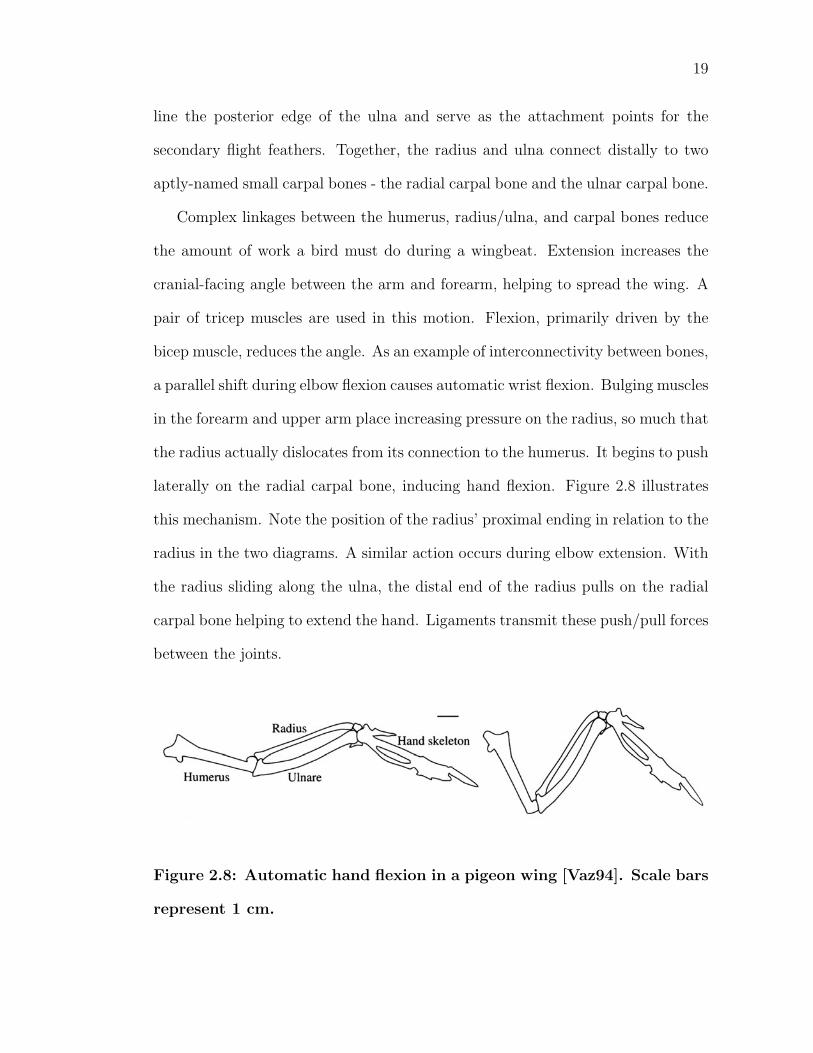
Complex linkages between the humerus, radius/ulna, and carpal bones reduce

the amount of work a bird must do during a wingbeat. Extension increases the

cranial-facing angle between the arm and forearm, helping to spread the wing. A

pair of tricep muscles are used in this motion. Flexion, primarily driven by the

bicep muscle, reduces the angle. As an example of interconnectivity between bones,

a parallel shift during elbow flexion causes automatic wrist flexion. Bulging muscles

in the forearm and upper arm place increasing pressure on the radius, so much that

the radius actually dislocates from its connection to the humerus. It begins to push

laterally on the radial carpal bone, inducing hand flexion. Figure 2.8 illustrates

this mechanism. Note the position of the radius’ proximal ending in relation to the

radius in the two diagrams. A similar action occurs during elbow extension. With

the radius sliding along the ulna, the distal end of the radius pulls on the radial

carpal bone helping to extend the hand. Ligaments transmit these push/pull forces

between the joints.

Figure 2.8: Automatic hand flexion in a pigeon wing [Vaz94]. Scale bars

represent 1 cm.

20

However, the forearm’s range of motion in its other degrees of freedom varies

depending on the wing’s pose. The forearm can also be elevated or depressed

relative to the humerus, or rotated on its long axis. However, when the wing

is spread, the arrangement of the joint limits movement to mainly extension and

flexion. This is hypothesized to reduce the amount energy needed to keep the wing

flat and level against the forces of air resistance. When the wing folds, the forearm

rotates so that its distal end turns ventrally. Raising or lowering the distal ends

of the radius and ulna relative to each other creates such a rotation along the long

axis of the forearm. For instance, dorsal rotation involves raising the distal end of

the radius.

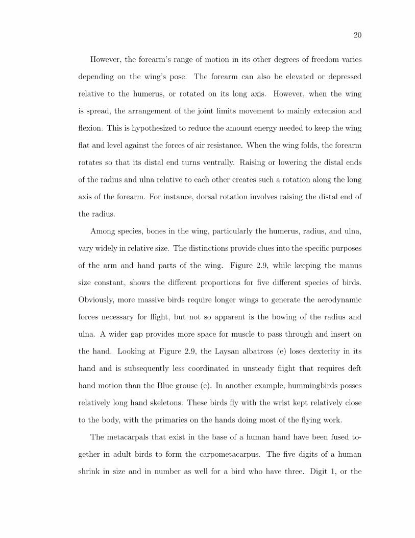
Among species, bones in the wing, particularly the humerus, radius, and ulna,

vary widely in relative size. The distinctions provide clues into the specific purposes

of the arm and hand parts of the wing. Figure 2.9, while keeping the manus

size constant, shows the different proportions for five different species of birds.

Obviously, more massive birds require longer wings to generate the aerodynamic

forces necessary for flight, but not so apparent is the bowing of the radius and

ulna. A wider gap provides more space for muscle to pass through and insert on

the hand. Looking at Figure 2.9, the Laysan albatross (e) loses dexterity in its

hand and is subsequently less coordinated in unsteady flight that requires deft

hand motion than the Blue grouse (c). In another example, hummingbirds posses

relatively long hand skeletons. These birds fly with the wrist kept relatively close

to the body, with the primaries on the hands doing most of the flying work.

The metacarpals that exist in the base of a human hand have been fused to-

gether in adult birds to form the carpometacarpus. The five digits of a human

shrink in size and in number as well for a bird who have three. Digit 1, or the

21

Figure 2.9: Relative sizes for the forelimb skeleton of five species of birds

[Dia92]. (a) Calliope hummingbird. (b) Rock dove. (c) Blue grouse.

(d) European starling. (e) Laysan albatross.

alular digit, inserts at the radial carpal bone and carpometacarpus joint. Com-

posed of two phalanges, it supports the specialized alula flight feathers. Digit 2, or

the major digit, is located at the distal end of the carpometacarpus. It consists of

the three phalanges, but the first two are fused. Only one phalanx forms the last

digit, the minor digit, which is located at the posterior end of the joint between

the carpometacarpus and the first phalanx of the second digit.

The carpal joint provides movement for the manus relative to the forearm,

and like the forearm is constrained by the shapes of the joints. Again, looking

at a spread wing as a level plane, the carpometacarpus, carpal bones, radius, and

ulna mainly restrain any movement outside of the plane. Movement of the manus

cranially is termed extension of the joint. Extensor muscles originate from the

distal end of the humerus and insert on the carpometacarpus. With similar flexor

22

muscles producing flexion, these sets of muscles create elevation, depression, and

rotation of the manus along its long axis only as a secondary effect.

Although the digits themselves are small in size and in number, even their tini-

est movements are large contributors to flight because they serve as attachment

points for several important feathers. However, their movements are highly re-

strained because of ligaments. The alular digit, even though it is the most mobile,

is only capable of extension (which raises the alular feathers away from the wing)

or flexion (which tucks them against the wing). The remaining digits mainly move

together as a group. Since the extra long distal primaries are attached to these

digits, small amounts of extension and flexion drastically change the wing’s surface

area. The digit at the end of the carpometacarpus can also rotate along its long

axis, which in turn raises or lowers the leading edge of the primaries.

In addition to the previously mentioned adaptations, wings include a feathered,

triangular shaped fold of skin called the propatagium (often referred to as just the

patagium) [BBK94, BBK95]. Stretching between the shoulder and wrist joints,

the patagium increases the surface area to generate extra lift for an unfurled wing.

Folding a wing tucks the patagium away to prevent damage. The tendon of the m.

tensor propatagialis pars longa provides the primary support (Figure 2.10). Some

debate actually exists as to whether or not this should be classified as a muscle

or as a ligament, but this thesis will use the muscle description. The m. tensor

propatagialis pars longa arises generally in the dorsal shoulder area, specifically on

head of the clavicle and sometimes the adjacent coracoid and scapula. Distally,

the tendon inserts on the carpometacarpus and wrist carpal bones. Only a portion

of the fiber, the pars elastica (in Figure 2.11, marked in gray), is stretchable; the

remainder is rigid. Given that the flexible portion is in the middle of the gap be-

23

tween the shoulder and wrist, a patagium would be unable to maintain a straight

leading edge without some sort of support. A propatagial strut (labeled PS in Fig-

ure 2.11), made out of strong collagenous fibers, extends from the elbow joint area

and connects to the pars elastica. Together, this system of musculature relaxes and

tenses the patagium as necessary during varying degrees of wing extension. As the

wing is flexed from its maximum flying length, the distance from the shoulder joint

to the wrist joint (called the mid-antebrachial chord) increases by approximately

30 percent. However, unlike how a rubber band gets thinner under tension, the

cross-sectional thickness of the patagial skin itself barely changes under stretching.

Additionally, as seen in Figure 2.10 as well, the patagial tendon also aids in the

automatic drawing motion of the hand.

2.3.4 Hindlimb Skeleton

The bird’s hindlimb skeleton is laid out in a pattern much like other vertebrates

(Figure 2.12). A typical femur, the largest of the bones in the leg, begins the

hindlimb skeleton. Attached to the ilium of the pelvis with a ball-socket joint, it is

capable of being swung cranially and caudally, as well as proximally and medially.

Rotation along an axis that passes through the femur is also possible. Continuing,

the knee joint and its associated patella bone (kneecap) connects the femur to the

tibiotarsus and a small fibula. Normally tucked tightly against the body, the knee

is often times not readily discernable to the naked eye, lying hidden underneath

the bird’s sleek exterior. Unlike a normal hinge joint which only allows one degree

of freedom, a bird’s knee allows for the same three degrees of freedom as the femur.

However, rotation about its long axis and the lateral-medial swing are secondary

to cranially-directed extension and caudially-directed flexion.

24

Figure 2.10: The m. tensor propatagialis pars longa, the narrow red

band running from the shoulder to the wrist, provides the main sup-

port for the patagium [Bur90]. Although relaxed when the wing is

folded, wing spreading increases tension in the muscle, helping to keep

a straight leading edge when the wing is extended. A secondary function

of the patagial muscle aids in automatic wrist extension.

Figure 2.11: A complete schematic of fibers in the patagium [BBK94].

25

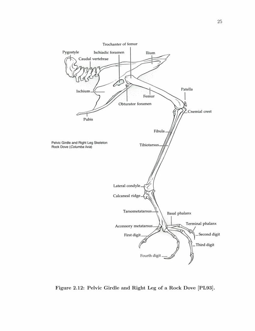
Figure 2.12: Pelvic Girdle and Right Leg of a Rock Dove [PL93].

26

Birds are known as digitigrade walkers, meaning they walk just on their toes.

The next bone downwards, the tarsometatarsus, would normally be the base of the

foot. As opposed to humans, where it extends from the ankle joint horizontally,

keeping in contact with the ground during at least some portion of the human walk

cycle, the tarsometatarsus in birds has a vertical orientation. Thus, the “ankle”

joint is actually off the ground entirely, causing it to be often confused as the knee.

Neverthless, movement about the ankle joint is the only way a bird can move its

toes as one unit. Range of motion and the mobility in each degree of freedom for

the ankle joint is similar to the knee joint. Additionally, the tarsometatarsus is

relatively long compared to other vertebrates. Extra length adds leverage when

leaping for takeoff as well as additional push when walking.

Most birds have four toes. The first digit is called the hallux and is analgous

to the human big toe. It consists of two phalanges. The second digit has three

phalanges, the third digit has four phalanges, and the fourth digit is the longest

with five phalanges. Keratinized claws are located on the most distal phalange

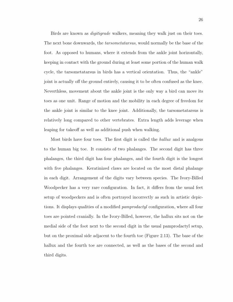
in each digit. Arrangement of the digits vary between species. The Ivory-Billed

Woodpecker has a very rare configuration. In fact, it differs from the usual feet

setup of woodpeckers and is often portrayed incorrectly as such in artistic depic-

tions. It displays qualities of a modified pamprodactyl configuration, where all four

toes are pointed cranially. In the Ivory-Billed, however, the hallux sits not on the

medial side of the foot next to the second digit in the usual pamprodactyl setup,

but on the proximal side adjacent to the fourth toe (Figure 2.13). The base of the

hallux and the fourth toe are connected, as well as the bases of the second and

third digits.

27

Figure 2.13: Ivory-Billed Woodpeckers display a rare configuration of

the foot where the three longer digits are pointed relatively forward and

the hallux is pointed nearly laterally [BM59].

28

2.3.5 Tail

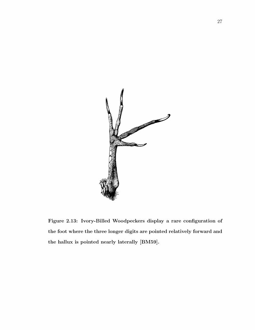
Figure 2.14: A Pileated Woodpecker uses his tail to balance himself on

the tree while perching. Adapted from [Soc05].

Primarily used as a control surface, the tail’s important functions are in braking

and steering. The long feathers on the tail, the rectrices, act as an air brake or

as a rudder in these situations. A spread tail also serves as an additional airfoil,

providing extra lift under slow-speed flight. Interestingly enough, the greatest

amount of variation in structrure and shape between species is seen in the tail;

each species has its own special secondary uses for the tail. Woodpeckers, with

extremely stiff rectrices, use their tail for support when perching vertically on a

tree (Figure 2.14). In other species, like the ostrich, the tail is a display mechanism.

As previously described, the tail skeleton is essentially the most caudal portion

of the vertebral column (Figure 2.15). It terminates at the pygostyle, to which

normally twelve (or six pairs) rectrices are attached. The pygostyle is actually

several vertebrae fused together early in embryonic development. Movements of

the caudal vertebral column cause the tail to move as a whole. Elevation above

29

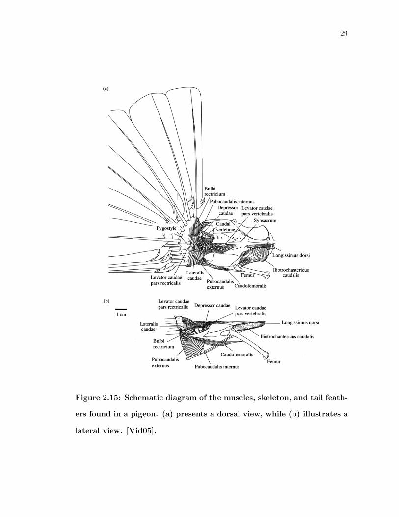
Figure 2.15: Schematic diagram of the muscles, skeleton, and tail feath-

ers found in a pigeon. (a) presents a dorsal view, while (b) illustrates a

lateral view. [Vid05].

30

and depression below the frontal plane are driven mainly by the levator caudae

and depressor caudae muscles, respectively. Additional accessory muscles also aid

in depression because, when the tail is lowered to act as an air brake, extra power

is needed to counteract the aerodynamic loads on the tail. The lateralis caudae

pushes the tail to one side or another within the frontal plane. Twisting along an

axis that passes through the vertebral column is also possible, and has the effect

of raising one side of the rectrices while lowering the other.

2.4 Feathers

Feathers are derived from the keratin scales of reptiles. Both form an overlapping

shield that protects the skin beneath [LS72]. All birds have a feather coat, and to

date, no other animals but birds have been found to posses feathers.

In most species of birds, feathers do not grow uniformly over the body. Though

they cover nearly the entire surface, feathers are attached in distinct tracts called

pterylae. Gaps between pterylae are called apteria.

2.4.1 Structure

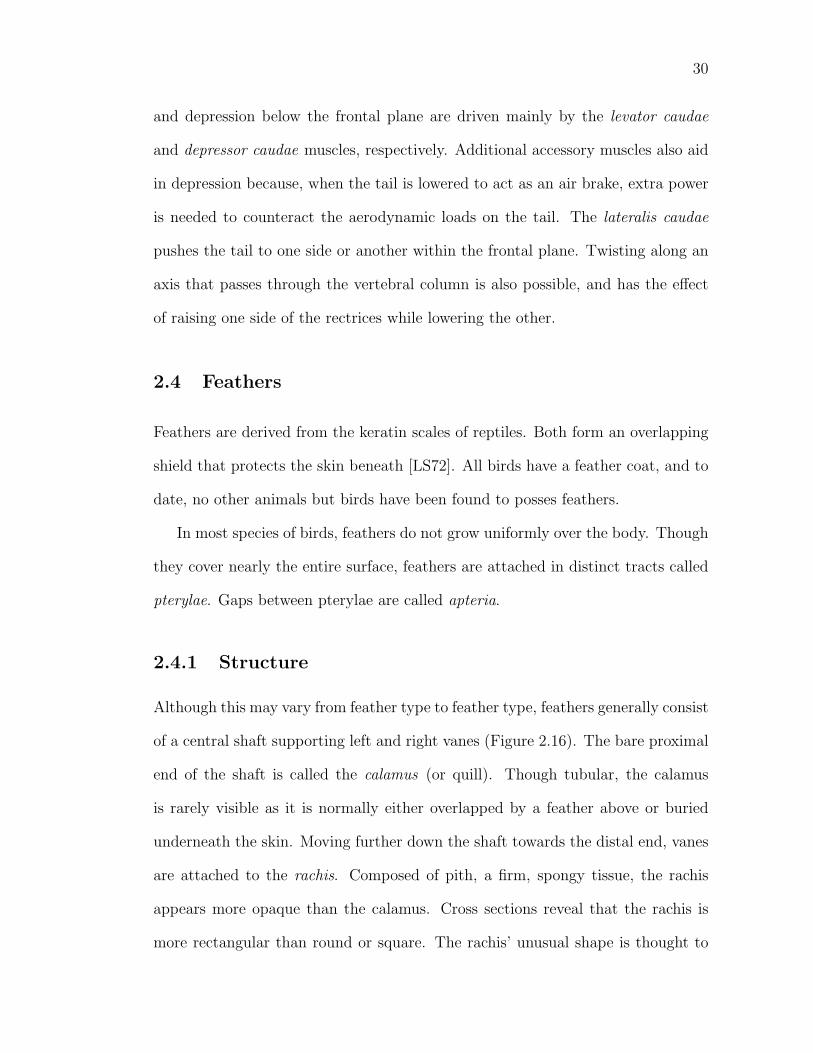
Although this may vary from feather type to feather type, feathers generally consist

of a central shaft supporting left and right vanes (Figure 2.16). The bare proximal

end of the shaft is called the calamus (or quill). Though tubular, the calamus

is rarely visible as it is normally either overlapped by a feather above or buried

underneath the skin. Moving further down the shaft towards the distal end, vanes

are attached to the rachis. Composed of pith, a firm, spongy tissue, the rachis

appears more opaque than the calamus. Cross sections reveal that the rachis is

more rectangular than round or square. The rachis’ unusual shape is thought to

31

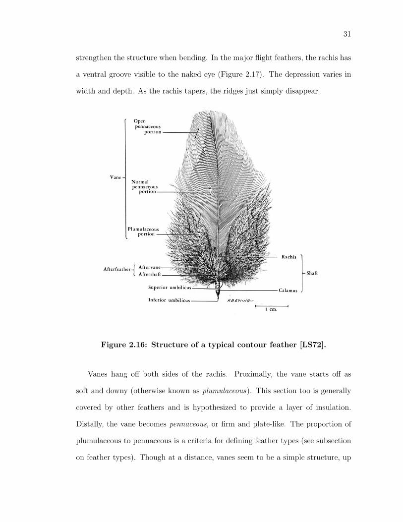
strengthen the structure when bending. In the major flight feathers, the rachis has

a ventral groove visible to the naked eye (Figure 2.17). The depression varies in

width and depth. As the rachis tapers, the ridges just simply disappear.

Figure 2.16: Structure of a typical contour feather [LS72].

Vanes hang off both sides of the rachis. Proximally, the vane starts off as

soft and downy (otherwise known as plumulaceous). This section too is generally

covered by other feathers and is hypothesized to provide a layer of insulation.

Distally, the vane becomes pennaceous, or firm and plate-like. The proportion of

plumulaceous to pennaceous is a criteria for defining feather types (see subsection

on feather types). Though at a distance, vanes seem to be a simple structure, up

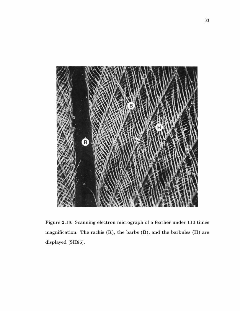
32

Figure 2.17: Closeup of a feather rachis [LS72].

close they have a complex hierarchical arrangment. Each vane itself is made up

of a collection of parallel barbs (marked with a B in Figure 2.18). Down another

level, each barb has lots of tiny branches called barbules (marked with an H in

Figure 2.18). Unless two neighboring barbs are separated, barbules are small

enough to be difficult to see with the naked eye. When two barbs are linked, their

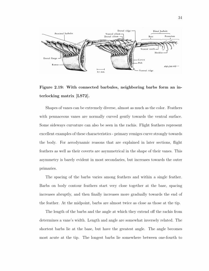
barbules arrange themselves in a pattern to fasten the barbs together (Figure 2.19).

The cross sections of proximal barbules look almost like exaggerated commas, with

a dorsal flange at the top edge. Hooklets on distal barbules latch onto the flanges

of neighboring proximal-facing barbules. Working almost like a zipper or Velcro,

the result is an interlocking surface (Figure 2.20). Birds can often be seen preening

their flight feathers, running their feathers through their bill, snapping together

adjacent barbules to ensure the largest continuous surface area possible.

33

Figure 2.18: Scanning electron micrograph of a feather under 110 times

magnification. The rachis (R), the barbs (B), and the barbules (H) are

displayed [SH85].

34

Figure 2.19: With connected barbules, neighboring barbs form an in-

terlocking matrix [LS72].

Shapes of vanes can be extremely diverse, almost as much as the color. Feathers

with pennaceous vanes are normally curved gently towards the ventral surface.

Some sideways curvature can also be seen in the rachis. Flight feathers represent

excellent examples of these characteristics - primary remiges curve strongly towards

the body. For aerodynamic reasons that are explained in later sections, flight

feathers as well as their coverts are asymmetrical in the shape of their vanes. This

asymmetry is barely evident in most secondaries, but increases towards the outer

primaries.

The spacing of the barbs varies among feathers and within a single feather.

Barbs on body contour feathers start very close together at the base, spacing

increases abruptly, and then finally increases more gradually towards the end of

the feather. At the midpoint, barbs are almost twice as close as those at the tip.

The length of the barbs and the angle at which they extend off the rachis from

determines a vane’s width. Length and angle are somewhat inversely related. The

shortest barbs lie at the base, but have the greatest angle. The angle becomes

most acute at the tip. The longest barbs lie somewhere between one-fourth to

35

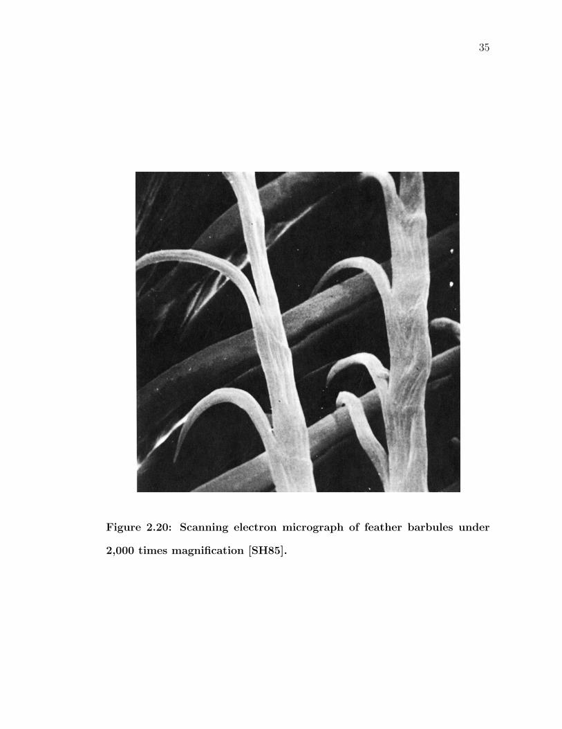
Figure 2.20: Scanning electron micrograph of feather barbules under

2,000 times magnification [SH85].

36

one-third of the rachis length. Barb length then stays constant for a short distance

and then gradually decreases near the tip. Primary feathers are often described as

emarginate, where the width decreases abruptly. This can happen at the narrower

leading edge vane, or the wider trailing edge vane, or both simultaneously. The

rate of decrease also determines the shape of the tip. Primaries often have obtuse

tips that are blunt and rounded off. Secondaries and rectrices are more truncated,

looking like a square end that’s been cut off.

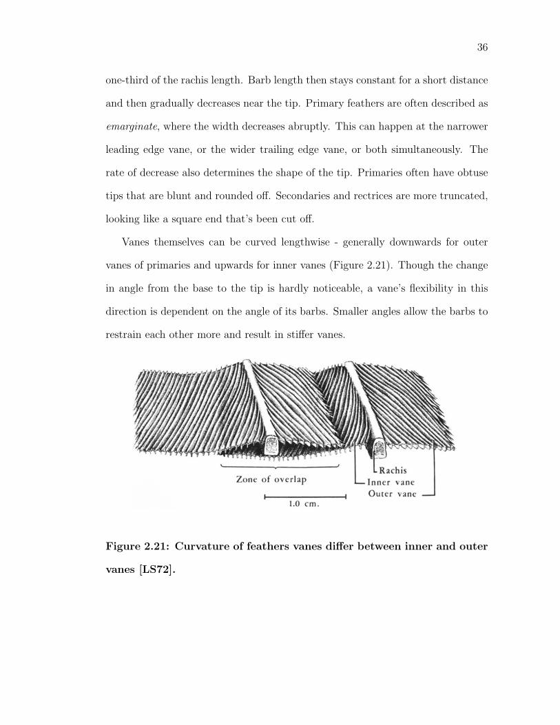
Vanes themselves can be curved lengthwise - generally downwards for outer

vanes of primaries and upwards for inner vanes (Figure 2.21). Though the change

in angle from the base to the tip is hardly noticeable, a vane’s flexibility in this

direction is dependent on the angle of its barbs. Smaller angles allow the barbs to

restrain each other more and result in stiffer vanes.

Figure 2.21: Curvature of feathers vanes differ between inner and outer

vanes [LS72].

37

2.4.2 Feather Appearance

Just like any other material, how a feather responds to incident light determines its

visual appearance. It can reflect light in three different manners: pigment-based,

structural coloration, and spectrally unselective specular reflection.

Spectrally unselective specular reflection is the easiest of the three to discuss;

it results in a white highlight. Reflection, to at least some extent, is dependent

on the macro geometry of the feather, including the lengthwise curvature of the

vanes, for all three reflection modes. It is particularly important here. Typically,

highlights generally run perpendicularly to barb curvature along its length (similar

to observations made in hair fibers). Less obvious is the dependence on the cross-

sectional shape of the barbs. A close-up look at a barb reveals that the dorsal

and ventral sides, or ridges, are not exactly the same (Figure 2.22). Dorsal ridges

tend to be more pointed, while ventral ridges appear flatter. This difference in the

amount of flat surface area may explain the observation that highlights generally

tend to be stronger when viewing the feather ventrally. Cross sectional profiles

will change proximally/distally along a barb, as seen in C and D of Figure 2.22,

modifying the observed highlight. In addition, shapes also vary across species,

so not all species will exhibit the same amount of spectrally unselective specular

reflection.

The other modes of reflection require some background on the structure of a

barb. When viewed from a cross section, a large sack, or vacuole, of air sits at the

center. A layer of pigment granules, or chemical compounds that produce color,

usually immediately line the vacuole. Next comes a medullary layer, comprised of

smaller air vacuoles and keratin rods. Keratin is the same durable protein found in

human hair. Because feather vanes must resist aerodynamic forces and maintain

38

Figure 2.22: Cross sections of feather barbs from A. Single Comb White

Leghorn Chicken’s secondary B. Yellow-shafted Flicker’s primary C.

proximal end of a Common Crow’s primary D. distal end of a Com-

mon Crow’s primary [LS72].

39

their shape during flight, feathers contain a different, even stronger, form of keratin.

As evident in the TEM photographs (Figure 2.23), this medullary layer resembles

a sponge, lacking organization in any predictable fashion. Finally, a cortical layer

of cells envelope the entire barb.

Figure 2.23: Cross-sectional transmission electron micrograph of a

feather barb. The left panel describes how a barb consists of mainly

a large vacuole (v) surrounded by melanin (m), a matrix of keratin (k)

and cell walls (cw), and the barb cortex (c). The right panel is a closeup

of the keratin layer. The scale bar represents 500 nm. [PAT03].

Pigments absorb light of certain wavelengths. There are three general types of

pigments found in bird feathers: melanins, carotenoids, and porphyrins. Melanins,

the most common pigment, produce blacks, grays, dark browns, and other earth-

toned colors. Since the intensity of these colors is directly proportional to the

amount of melanin present [MSW05], the feathers of the Ivory-Billed Woodpecker

likely contain melanin in abundance. Melanin is also thought to add strength to

the feather, which explains why at least a small amount is present in all types

40

of feathers, particularly the flight feathers. In the presence of melanin granules,

additional keratin is deposited, resulting in a stiffer keratin/granule composite

[Tic03]. Thus, abrasion marks are much more common on the keratin deficient

white wing tips than on the keratin rich black wing tips. Responsible for producing

bright reds and yellows, carotenoids are most likely present on a male Ivory-Billed’s

red crown. Porphyrins create brown and redish-brown colors.

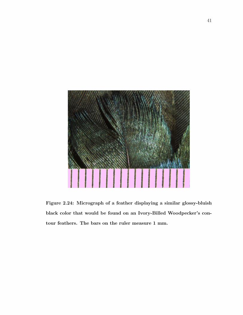
Structural coloration, which occur as a result of scattering in the spongy keratin

and air matrix, provides arguably the most interesting reflections. Since pigments

only create a few colors of the spectrum, a mixture of structural coloration and

pigmentation is reponsible for many of the colors seen in birds. An example of

this is the glossy-blue black color visible in the feathers that cover the Ivory-

Billed Woodpecker’s torso (Figure 2.24 and Figure 2.25). The actual mechanism

of how light produces these structural colors has been debated for the last thirty

years. Previously published research pointed at incoherent scattering models such

as Rayleigh and Mie scattering [Lan72, Fox76]. Examples in nature where these

types of scattering occur include blue sky, skim milk, and blue ice and snow. These

mechanisms predict that color is related only to the size and refractive index of

the scattering objects, causing varying effects on different portions of the spectrum

(top of Figure 2.26). These objects are assumed to be randomly distributed, and

thus, the phase relationships of scattered light can be ignored.

Recent work published only in the last few years by Richard Prum disproved the

incoherent scattering theory and provided evidence that indeed the phase relation-

ships do matter [PTWD98, PTWD99, PT03, PAT03]. Such scattering is known

as coherent scattering. Phase relationships are determined by the difference be-

tween the distances traveled by each of the incident light waves, called path-length

41

Figure 2.24: Micrograph of a feather displaying a similar glossy-bluish

black color that would be found on an Ivory-Billed Woodpecker’s con-

tour feathers. The bars on the ruler measure 1 mm.

42

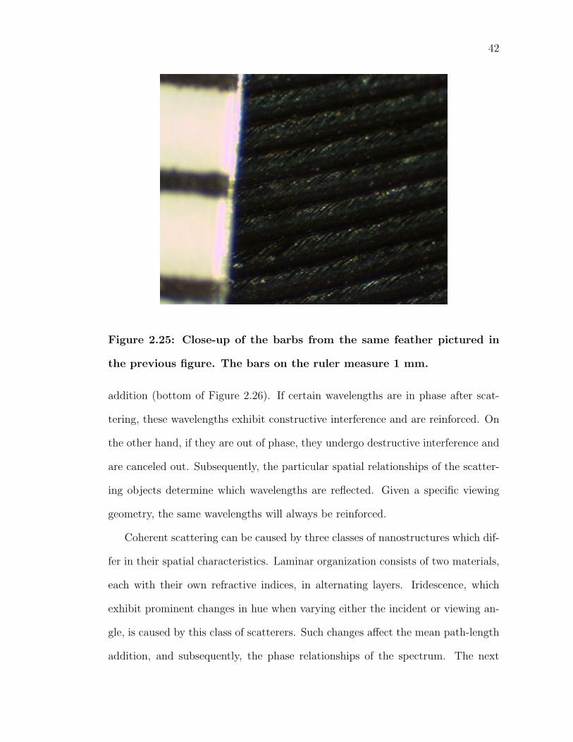
Figure 2.25: Close-up of the barbs from the same feather pictured in

the previous figure. The bars on the ruler measure 1 mm.

addition (bottom of Figure 2.26). If certain wavelengths are in phase after scat-

tering, these wavelengths exhibit constructive interference and are reinforced. On

the other hand, if they are out of phase, they undergo destructive interference and

are canceled out. Subsequently, the particular spatial relationships of the scatter-

ing objects determine which wavelengths are reflected. Given a specific viewing

geometry, the same wavelengths will always be reinforced.

Coherent scattering can be caused by three classes of nanostructures which dif-

fer in their spatial characteristics. Laminar organization consists of two materials,

each with their own refractive indices, in alternating layers. Iridescence, which

exhibit prominent changes in hue when varying either the incident or viewing an-

gle, is caused by this class of scatterers. Such changes affect the mean path-length

addition, and subsequently, the phase relationships of the spectrum. The next

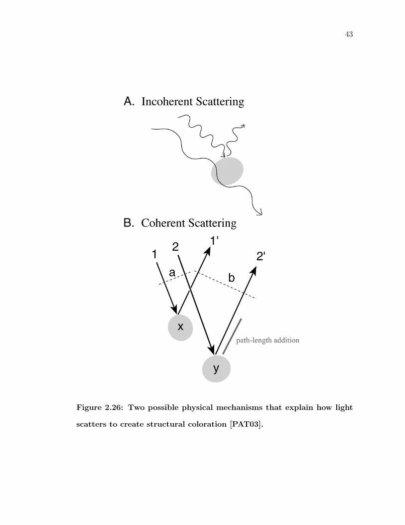
43

Figure 2.26: Two possible physical mechanisms that explain how light

scatters to create structural coloration [PAT03].

44

type of coherent scatterers, crystal-like, distributes its scatterers in a square or

hexagonal array.

The final class of coherent scatters fall into the general category of quasi-

ordered. Although seemingly unorganized, Prum’s work proved that the spongy,

medullary layer of keratin and air vacuoles do actually possess enough spatial

organization to produce coherent scattering. He relates the layer to “a bowl of

popcorn.” At large scales, it does indeed lack spatial ordering, explaining its in-

ability to produce strong iridescence. However, each keratin rod or air vacuole (or

popped kernel to use the Prum analogy) remain similar in size to its neighbor and

are separated by nearly the same distance. This kind of uniformity is enough to

produce structural coloration. Unlike iridescence, changes in viewing geometry do

not modify the color observed. Medullary keratin exists cylindrically in a feather

barb, so even large differences in the angle of incidence or viewing direction do not

vary the overall distribution of scatterers or path-lengths.

2.4.3 Feather Types

Six major types of feathers exist: contour, down, semi-plumulaceous, filoplumula-

ceous, powder, and bristle-like (Figure 2.27). While not all of these types are al-

ways visible, each serve a unique function. Some, like down and semi-plumulaceous

feathers, are hidden underneath the outer contour feathers to provide a layer of

warm insulation. Other types, like bristles, line the bird’s openings, such as the

eyes, nostrils, and mouth. They serve as tactile structures, much like a cat’s

whiskers. Filoplumes are accessory feathers that help birds determine the position

of the remiges and rectrices. Scattered at the base of the wing, each filoplumu-

laceous feather belongs to a small sense bud that can detect the filoplume’s fine

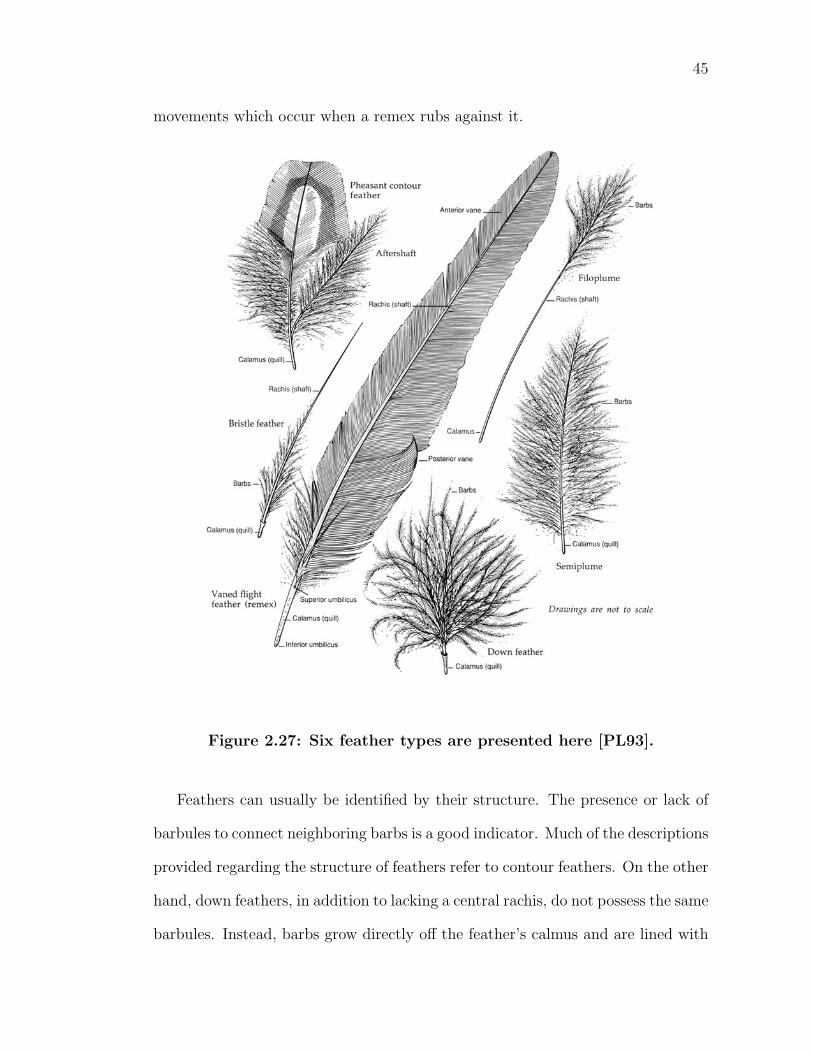
45

movements which occur when a remex rubs against it.

Figure 2.27: Six feather types are presented here [PL93].

Feathers can usually be identified by their structure. The presence or lack of

barbules to connect neighboring barbs is a good indicator. Much of the descriptions

provided regarding the structure of feathers refer to contour feathers. On the other

hand, down feathers, in addition to lacking a central rachis, do not possess the same

barbules. Instead, barbs grow directly off the feather’s calmus and are lined with

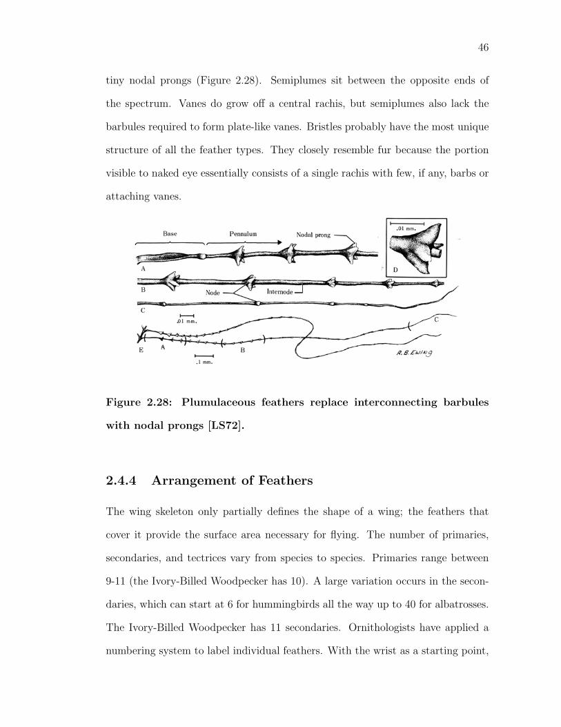
46

tiny nodal prongs (Figure 2.28). Semiplumes sit between the opposite ends of

the spectrum. Vanes do grow off a central rachis, but semiplumes also lack the

barbules required to form plate-like vanes. Bristles probably have the most unique

structure of all the feather types. They closely resemble fur because the portion

visible to naked eye essentially consists of a single rachis with few, if any, barbs or

attaching vanes.

Figure 2.28: Plumulaceous feathers replace interconnecting barbules

with nodal prongs [LS72].

2.4.4 Arrangement of Feathers

The wing skeleton only partially defines the shape of a wing; the feathers that

cover it provide the surface area necessary for flying. The number of primaries,

secondaries, and tectrices vary from species to species. Primaries range between

9-11 (the Ivory-Billed Woodpecker has 10). A large variation occurs in the secon-

daries, which can start at 6 for hummingbirds all the way up to 40 for albatrosses.

The Ivory-Billed Woodpecker has 11 secondaries. Ornithologists have applied a

numbering system to label individual feathers. With the wrist as a starting point,

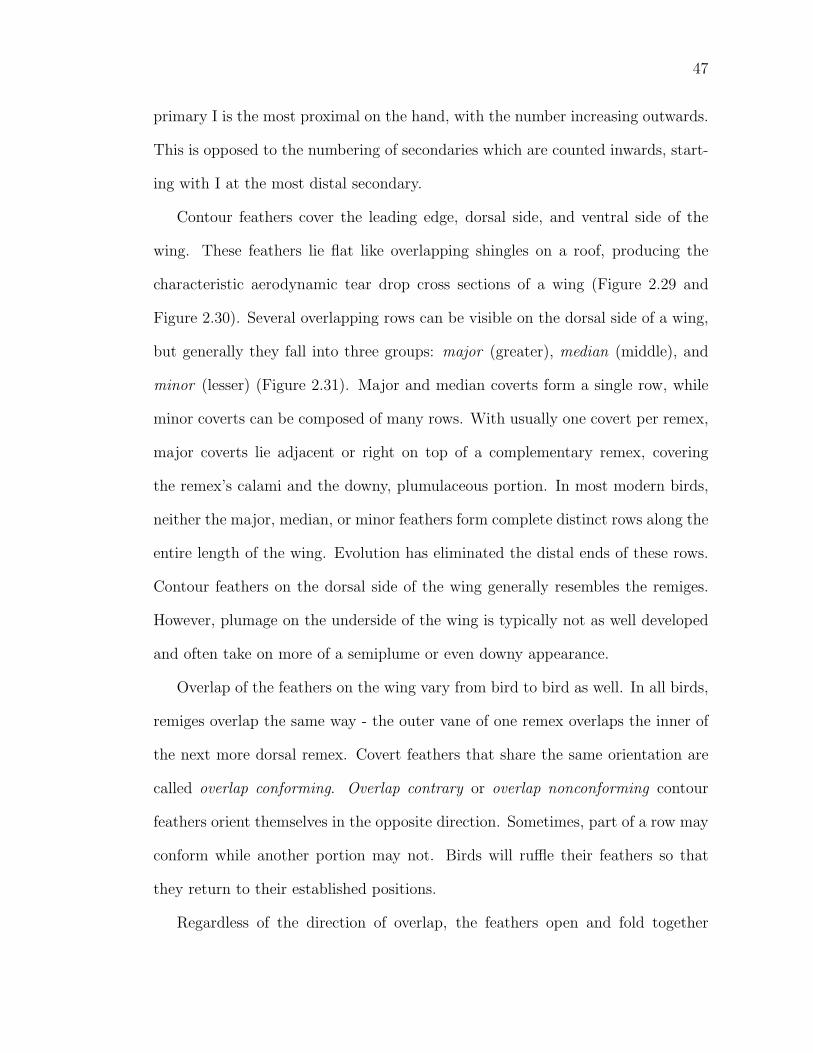
47

primary I is the most proximal on the hand, with the number increasing outwards.

This is opposed to the numbering of secondaries which are counted inwards, start-

ing with I at the most distal secondary.

Contour feathers cover the leading edge, dorsal side, and ventral side of the

wing. These feathers lie flat like overlapping shingles on a roof, producing the

characteristic aerodynamic tear drop cross sections of a wing (Figure 2.29 and

Figure 2.30). Several overlapping rows can be visible on the dorsal side of a wing,

but generally they fall into three groups: major (greater), median (middle), and

minor (lesser) (Figure 2.31). Major and median coverts form a single row, while

minor coverts can be composed of many rows. With usually one covert per remex,

major coverts lie adjacent or right on top of a complementary remex, covering

the remex’s calami and the downy, plumulaceous portion. In most modern birds,

neither the major, median, or minor feathers form complete distinct rows along the

entire length of the wing. Evolution has eliminated the distal ends of these rows.

Contour feathers on the dorsal side of the wing generally resembles the remiges.

However, plumage on the underside of the wing is typically not as well developed

and often take on more of a semiplume or even downy appearance.

Overlap of the feathers on the wing vary from bird to bird as well. In all birds,

remiges overlap the same way - the outer vane of one remex overlaps the inner of

the next more dorsal remex. Covert feathers that share the same orientation are

called overlap conforming. Overlap contrary or overlap nonconforming contour

feathers orient themselves in the opposite direction. Sometimes, part of a row may

conform while another portion may not. Birds will ruffle their feathers so that

they return to their established positions.

Regardless of the direction of overlap, the feathers open and fold together

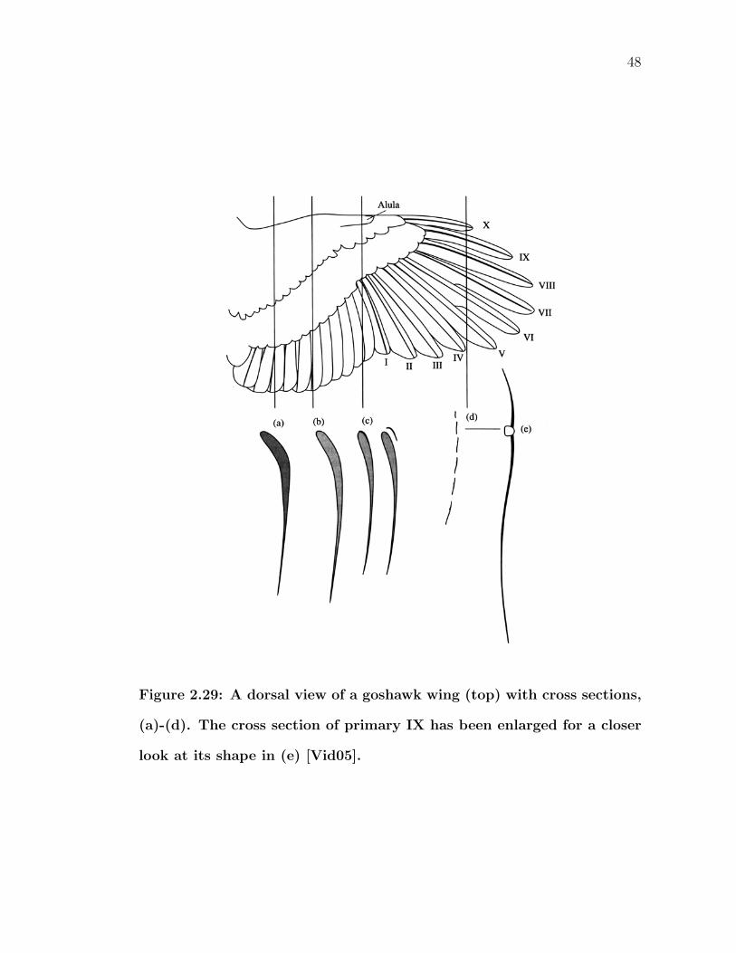
48

Figure 2.29: A dorsal view of a goshawk wing (top) with cross sections,

(a)-(d). The cross section of primary IX has been enlarged for a closer

look at its shape in (e) [Vid05].

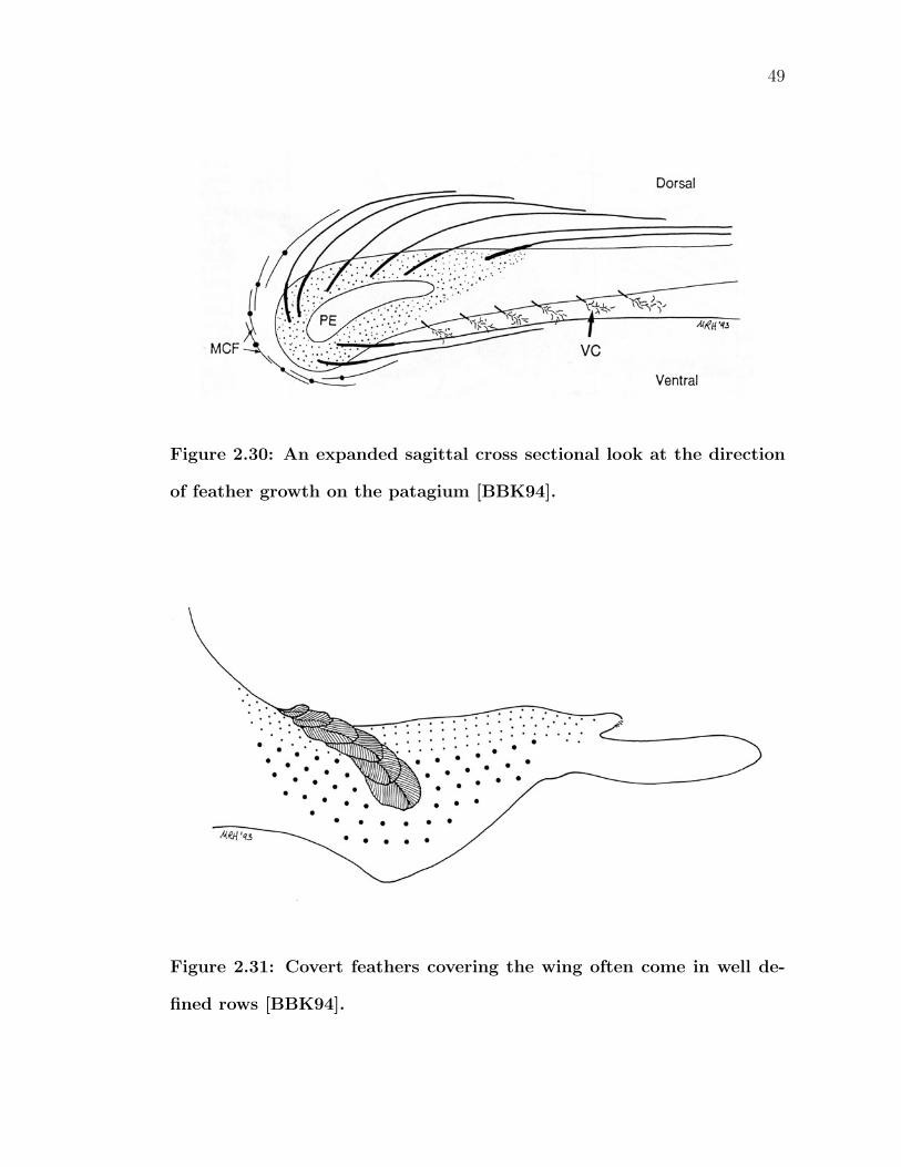
49

Figure 2.30: An expanded sagittal cross sectional look at the direction

of feather growth on the patagium [BBK94].

Figure 2.31: Covert feathers covering the wing often come in well de-

fined rows [BBK94].

50

compactly and without interference. The process of unfurling the remiges on a

wing resembles opening a deck of playing cards. Starting with a closed position,

secondaries overlap its proximal neighbor ventrally. The manus is flexed tightly

against the forearm, causing the primaries to slide underneath and disappear under

the secondaries. As the most important flight feathers, this arrangement provides

maximum protection for the primaries. Additionally, the digits are flexed tightly

such that the shafts of the primaries become parallel to each other. As the wing

spreads open, the remiges diverge from each other, increasing the surface area of

the wing. Though it may be difficult to discern from Figure 2.32 and Figure 2.33,

each feather, however, is always rotating at least a small amount at any given time

during wing spreading. With different limits to the amount of rotation, each feather

must rotate at different angular velocities to complete spreading within a given

amount of time. Since secondaries rotate only a small amount, they may appear

to be fairly rigidly attached. Meanwhile, primaries have a significant amount of

travel - movement in the outer primaries is visible all the way through the final

frames in Figures 2.32 and 2.33.

The actual mechanism that spreads the feathers on a wing is a combination

of ligaments and muscles (Figure 2.34). Secondaries enjoy a wide enough range

of movement such that they can swing proximally or distally without resistance.

However, distally, movement in the primaries becomes increasingly restricted. The

most distal primary, attached to the major digit, virtually has no movement in-

dependent of the digit. As the digit extends in wing spreading, the outer primary

swings along with it. The other primaries likewise follow because they are fairly

anchored to the digits and carpometacarpus. The interremigial ligament, which

begins at the elbow and runs laterally, thereby connecting the remiges, transmits

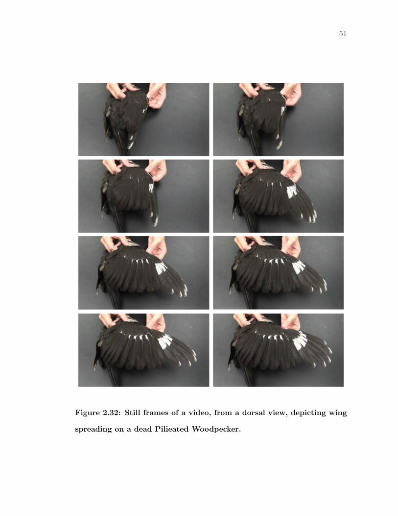
51

Figure 2.32: Still frames of a video, from a dorsal view, depicting wing

spreading on a dead Pilieated Woodpecker.

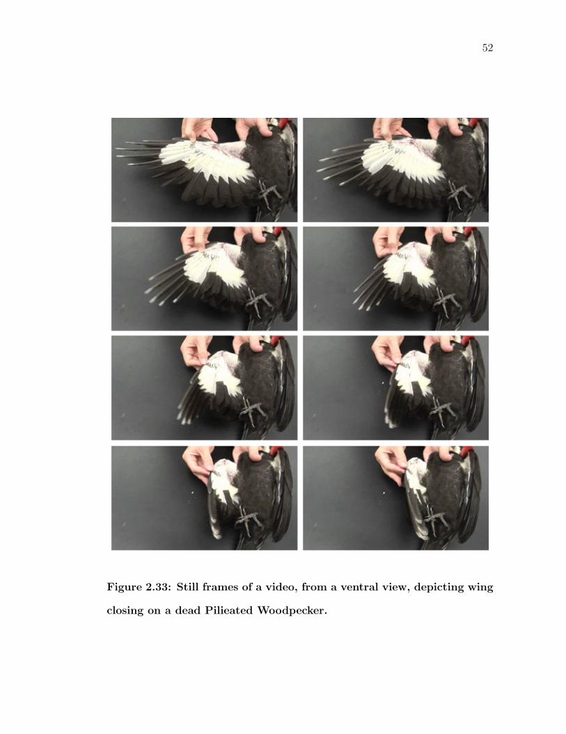
52

Figure 2.33: Still frames of a video, from a ventral view, depicting wing

closing on a dead Pilieated Woodpecker.

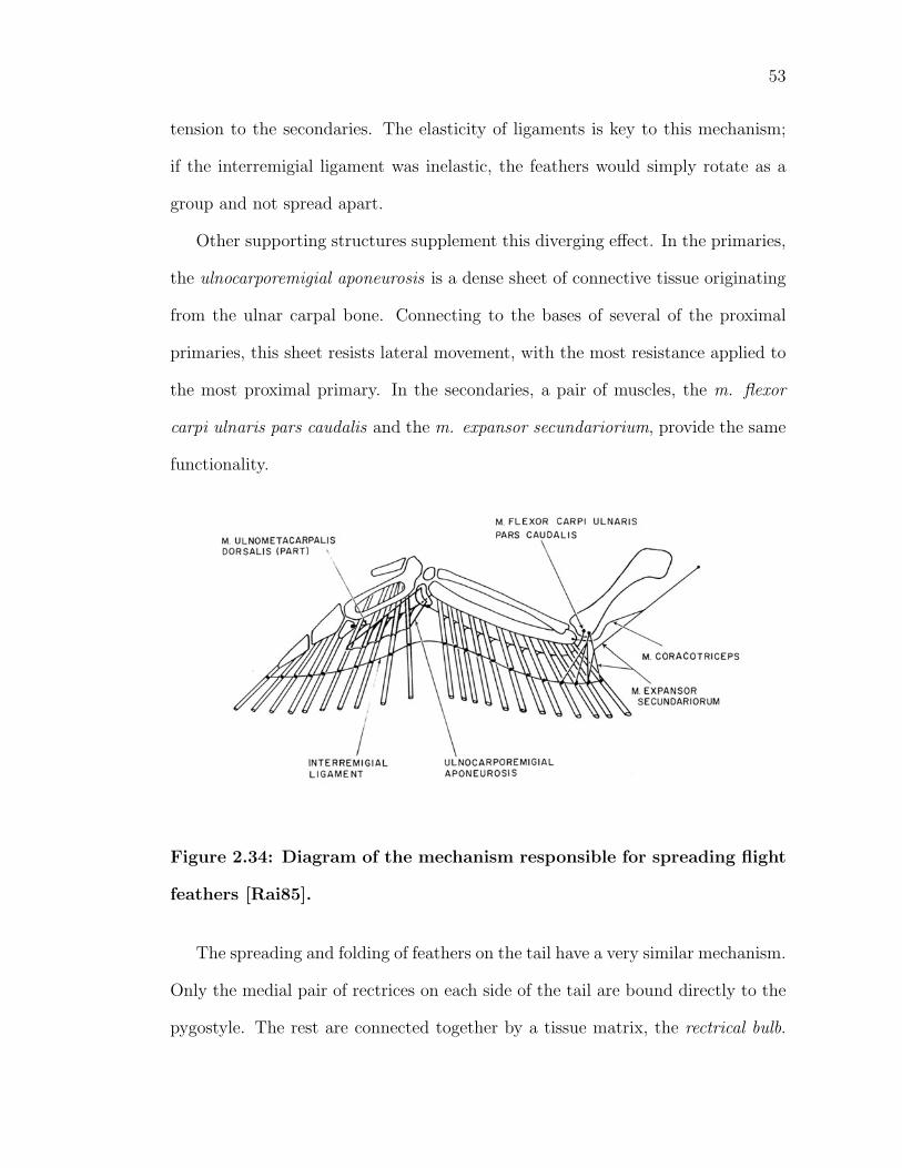
53

tension to the secondaries. The elasticity of ligaments is key to this mechanism;

if the interremigial ligament was inelastic, the feathers would simply rotate as a

group and not spread apart.

Other supporting structures supplement this diverging effect. In the primaries,

the ulnocarporemigial aponeurosis is a dense sheet of connective tissue originating

from the ulnar carpal bone. Connecting to the bases of several of the proximal

primaries, this sheet resists lateral movement, with the most resistance applied to

the most proximal primary. In the secondaries, a pair of muscles, the m. flexor

carpi ulnaris pars caudalis and the m. expansor secundariorium, provide the same

functionality.

Figure 2.34: Diagram of the mechanism responsible for spreading flight

feathers [Rai85].

The spreading and folding of feathers on the tail have a very similar mechanism.

Only the medial pair of rectrices on each side of the tail are bound directly to the

pygostyle. The rest are connected together by a tissue matrix, the rectrical bulb.

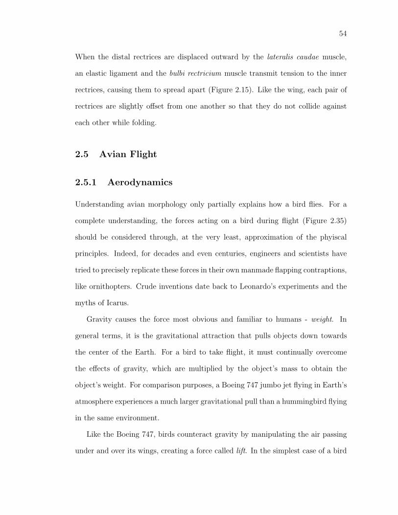
54

When the distal rectrices are displaced outward by the lateralis caudae muscle,

an elastic ligament and the bulbi rectricium muscle transmit tension to the inner

rectrices, causing them to spread apart (Figure 2.15). Like the wing, each pair of

rectrices are slightly offset from one another so that they do not collide against

each other while folding.

2.5 Avian Flight

2.5.1 Aerodynamics

Understanding avian morphology only partially explains how a bird flies. For a

complete understanding, the forces acting on a bird during flight (Figure 2.35)

should be considered through, at the very least, approximation of the phyiscal

principles. Indeed, for decades and even centuries, engineers and scientists have

tried to precisely replicate these forces in their own manmade flapping contraptions,

like ornithopters. Crude inventions date back to Leonardo’s experiments and the

myths of Icarus.

Gravity causes the force most obvious and familiar to humans - weight. In

general terms, it is the gravitational attraction that pulls objects down towards

the center of the Earth. For a bird to take flight, it must continually overcome

the effects of gravity, which are multiplied by the object’s mass to obtain the

object’s weight. For comparison purposes, a Boeing 747 jumbo jet flying in Earth’s

atmosphere experiences a much larger gravitational pull than a hummingbird flying

in the same environment.

Like the Boeing 747, birds counteract gravity by manipulating the air passing

under and over its wings, creating a force called lift. In the simplest case of a bird

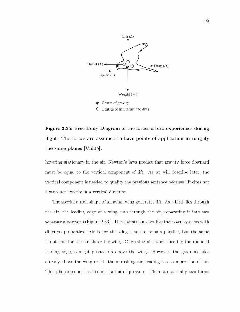
55

Figure 2.35: Free Body Diagram of the forces a bird experiences during

flight. The forces are assumed to have points of application in roughly

the same planes [Vid05].

hovering stationary in the air, Newton’s laws predict that gravity force downard

must be equal to the vertical component of lift. As we will describe later, the

vertical component is needed to qualify the previous sentence because lift does not

always act exactly in a vertical direction.

The special airfoil shape of an avian wing generates lift. As a bird flies through

the air, the leading edge of a wing cuts through the air, separating it into two

separate airstreams (Figure 2.36). These airstreams act like their own systems with

different properties. Air below the wing tends to remain parallel, but the same

is not true for the air above the wing. Oncoming air, when meeting the rounded

leading edge, can get pushed up above the wing. However, the gas molecules

already above the wing resists the onrushing air, leading to a compression of air.

This phenomenon is a demonstration of pressure. There are actually two forms

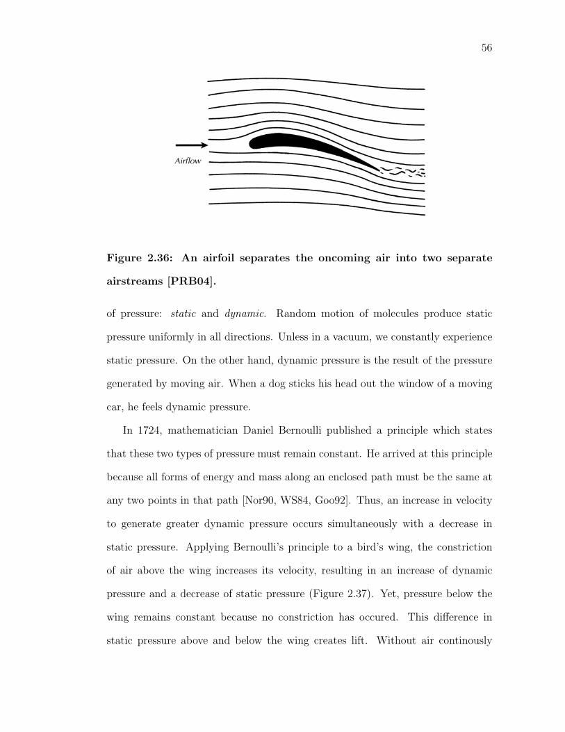
56

Figure 2.36: An airfoil separates the oncoming air into two separate

airstreams [PRB04].

of pressure: static and dynamic. Random motion of molecules produce static

pressure uniformly in all directions. Unless in a vacuum, we constantly experience

static pressure. On the other hand, dynamic pressure is the result of the pressure

generated by moving air. When a dog sticks his head out the window of a moving

car, he feels dynamic pressure.

In 1724, mathematician Daniel Bernoulli published a principle which states

that these two types of pressure must remain constant. He arrived at this principle

because all forms of energy and mass along an enclosed path must be the same at

any two points in that path [Nor90, WS84, Goo92]. Thus, an increase in velocity

to generate greater dynamic pressure occurs simultaneously with a decrease in

static pressure. Applying Bernoulli’s principle to a bird’s wing, the constriction

of air above the wing increases its velocity, resulting in an increase of dynamic

pressure and a decrease of static pressure (Figure 2.37). Yet, pressure below the

wing remains constant because no constriction has occured. This difference in

static pressure above and below the wing creates lift. Without air continously

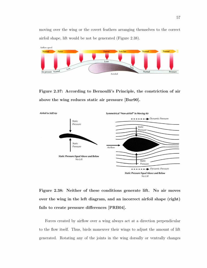
57

moving over the wing or the covert feathers arranging themselves to the correct

airfoil shape, lift would be not be generated (Figure 2.38).

Figure 2.37: According to Bernoulli’s Principle, the constriction of air

above the wing reduces static air pressure [Bur90].

Figure 2.38: Neither of these conditions generate lift. No air moves

over the wing in the left diagram, and an incorrect airfoil shape (right)

fails to create pressure differences [PRB04].

Forces created by airflow over a wing always act at a direction perpendicular

to the flow itself. Thus, birds maneuver their wings to adjust the amount of lift

generated. Rotating any of the joints in the wing dorsally or ventrally changes

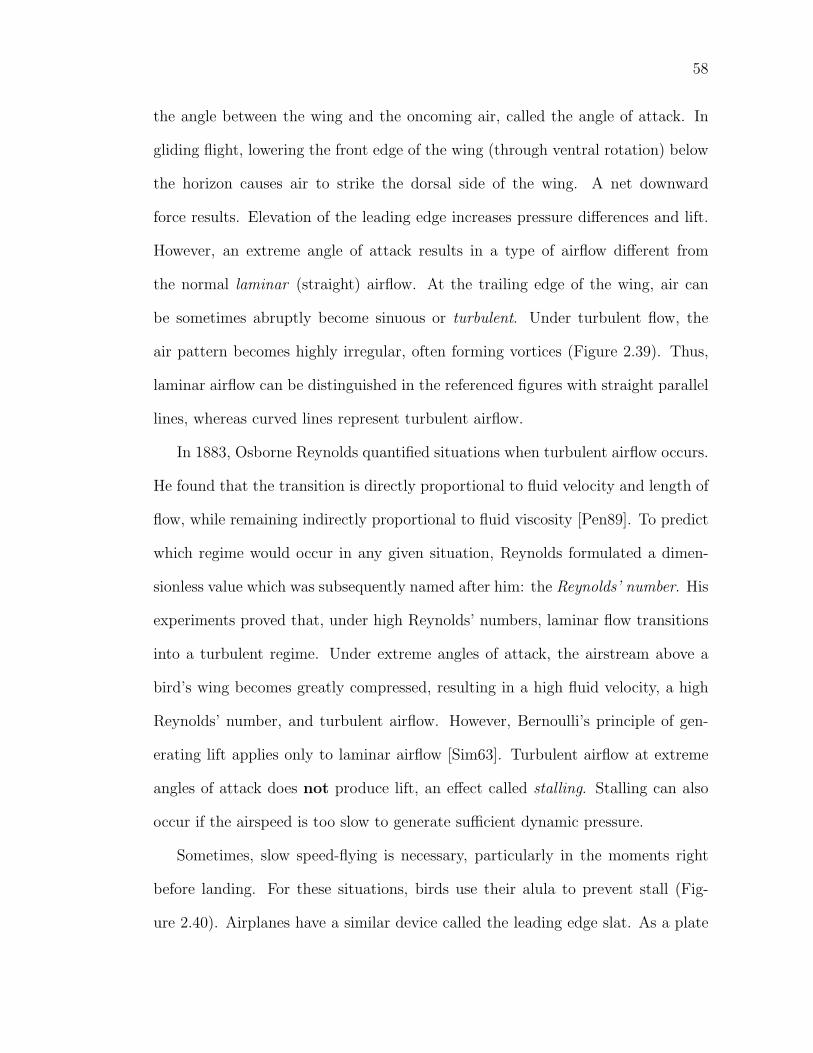
58

the angle between the wing and the oncoming air, called the angle of attack. In

gliding flight, lowering the front edge of the wing (through ventral rotation) below

the horizon causes air to strike the dorsal side of the wing. A net downward

force results. Elevation of the leading edge increases pressure differences and lift.

However, an extreme angle of attack results in a type of airflow different from

the normal laminar (straight) airflow. At the trailing edge of the wing, air can

be sometimes abruptly become sinuous or turbulent. Under turbulent flow, the

air pattern becomes highly irregular, often forming vortices (Figure 2.39). Thus,

laminar airflow can be distinguished in the referenced figures with straight parallel

lines, whereas curved lines represent turbulent airflow.

In 1883, Osborne Reynolds quantified situations when turbulent airflow occurs.

He found that the transition is directly proportional to fluid velocity and length of

flow, while remaining indirectly proportional to fluid viscosity [Pen89]. To predict

which regime would occur in any given situation, Reynolds formulated a dimen-

sionless value which was subsequently named after him: the Reynolds’ number. His

experiments proved that, under high Reynolds’ numbers, laminar flow transitions

into a turbulent regime. Under extreme angles of attack, the airstream above a

bird’s wing becomes greatly compressed, resulting in a high fluid velocity, a high

Reynolds’ number, and turbulent airflow. However, Bernoulli’s principle of gen-

erating lift applies only to laminar airflow [Sim63]. Turbulent airflow at extreme

angles of attack does not produce lift, an effect called stalling. Stalling can also

occur if the airspeed is too slow to generate sufficient dynamic pressure.

Sometimes, slow speed-flying is necessary, particularly in the moments right

before landing. For these situations, birds use their alula to prevent stall (Fig-

ure 2.40). Airplanes have a similar device called the leading edge slat. As a plate

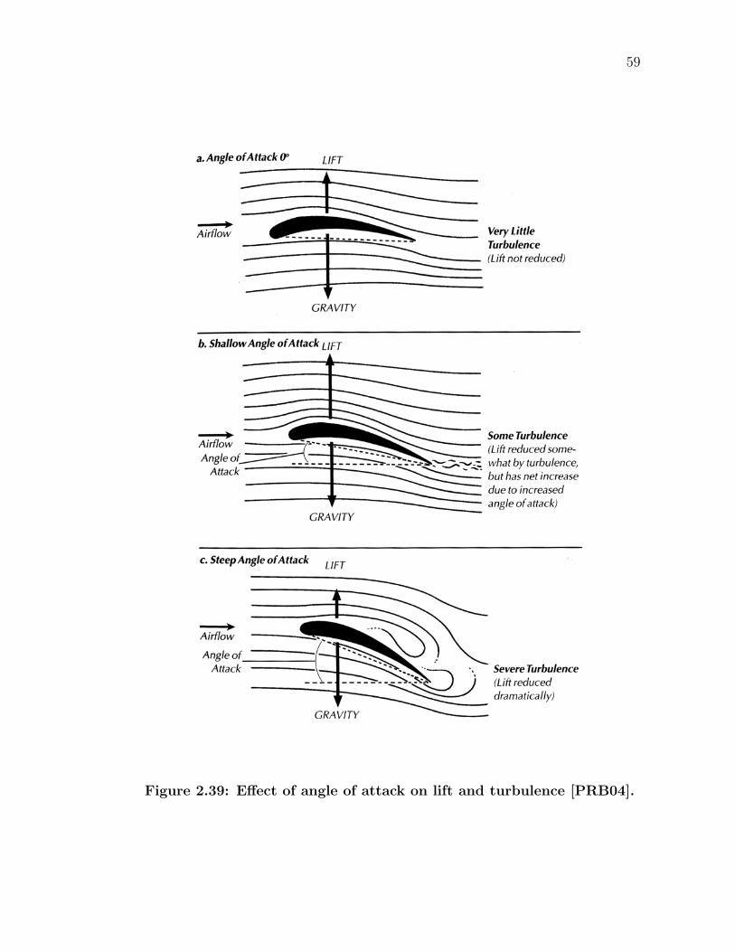
59

Figure 2.39: Effect of angle of attack on lift and turbulence [PRB04].

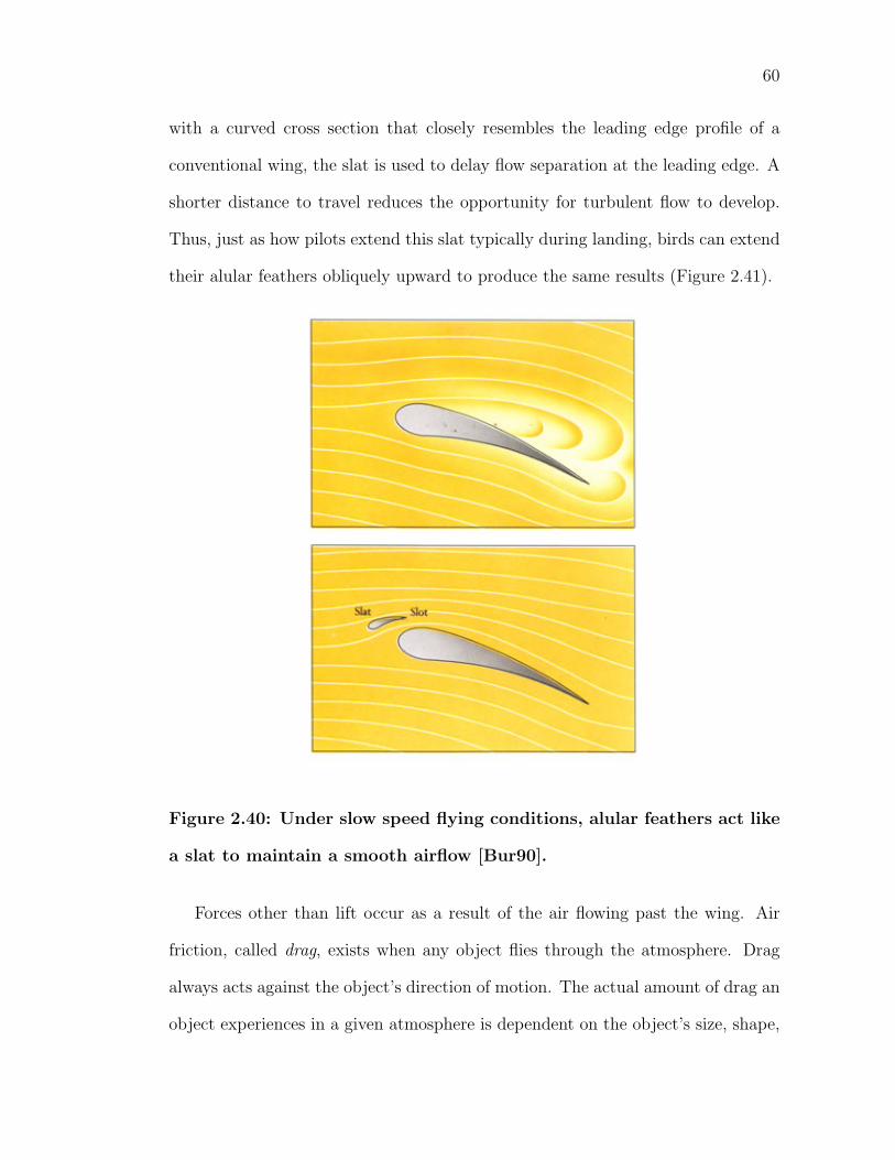
60

with a curved cross section that closely resembles the leading edge profile of a

conventional wing, the slat is used to delay flow separation at the leading edge. A

shorter distance to travel reduces the opportunity for turbulent flow to develop.

Thus, just as how pilots extend this slat typically during landing, birds can extend

their alular feathers obliquely upward to produce the same results (Figure 2.41).

Figure 2.40: Under slow speed flying conditions, alular feathers act like

a slat to maintain a smooth airflow [Bur90].

Forces other than lift occur as a result of the air flowing past the wing. Air

friction, called drag, exists when any object flies through the atmosphere. Drag

always acts against the object’s direction of motion. The actual amount of drag an

object experiences in a given atmosphere is dependent on the object’s size, shape,

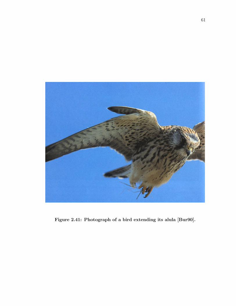
61

Figure 2.41: Photograph of a bird extending its alula [Bur90].

62

surface roughness, and projected surface area. Coefficients of drag summarize this

relationship numerically.

In the same way as lift counteracts gravity, a force must exist for a bird to sus-

tain forward flight over long distances: thrust. Thrust is the same physical force

that powers a moon rocket on its way into space. A Saturn V rocket shoots hot

gases out of the rear nozzle at high velocities. According to Newton’s Second and

Third Law of Motion, the gas accelerated in one direction causes an equal and op-

posite force on the rocket. A bird propels itself forward using the same principles.

During a typical powered flight wingbeat, the wing not only flaps up and down,

but also backwards and forwards, moving air horizontally. The specifics of how a

wingbeat propels a bird will be more accurately described in the following subsec-

tion, Section 2.5.2. However, note the important the interrelationship between lift

and thrust. Forward thrust is generally reponsible for moving air across the wings

to create lift. A bird producing insufficient thrust to overcome its own drag not

only slows down, but also then loses lift, and eventually descends. The opposite

is also true: when a bird’s thrust greatly exceeds its drag, it not only flies faster,

but also produces more lift causing the bird to ascend.

2.5.2 “Flythrough” of a Single Wingbeat

Having explained both the morphology (Section 2.3.3) and the physical forces

(Section 2.5.1), a closer examination of what happens during a wingbeat provides

together an answer to the question, “How does a bird fly?”. The walkthrough

presented here is the synthesis of numerous kinematic and aerodynamic studies

on avian flight using exotic procedures such as high x-ray cineradiography of an

European Starling flying in a wind tunnel by Kenneth Dial [DGJ91].

63

Using the terminology Dial used in his widely-cited 1991 paper, four phases

represent a wingbeat cycle: downstroke, downstroke-upstroke transition, upstroke,

and upstroke-downstroke transition (Figure 2.42). Downstroke lasts longer than

upstroke, taking up 53.5% of the cycle for a European Starling.

Downstroke, mainly characterized by humerus elevation and depression, re-

quires power generated from the pectoral girdle. At the onset of downstroke,

pectoral muscles, such as m. supracoracoideus in particular, has already elevated

the humerus to about 80-90 degrees above horizontal. The depressor muscles, such

as the m. pectoralis, then start to generate the characteristic up and down flap-

ping motion [DKG88]. The forces generated by the pectoralis actually widen the

furcula, storing potential energy that will later be used during upstroke to elevate

the wings (Figure 2.43) [JJDGJ88]. Thus, the furcula acts like a spring during a

wingbeat. The spreading of the wishbone also causes other changes in the pectoral

girdle since all the bones are joined together (Figure 2.44). The humerus moves

the same distance laterally. Since each head in the wishbone is attached to a cora-

coid, the coracoid rotates and slides at its attachment point to the sternum. The

scapula rotates as well, through an axis about two thirds of the way down the bone

posteriorly.

Meanwhile, the humerus is also protracted to roughly 55 degrees, where it

will remain until the downstroke-upstroke transition. One should note that this

measurement is expressed in terms of the angle between the long axis of the bone

and the longitudinal axis of the body. Elbow and wrist joints start extended to

nearly right angles, but will continue extending to about a maximum of 110-120

degrees and 150-160 degrees, respectively.

Secondary feathers keep the bird aloft throughout downstroke. In fact, the

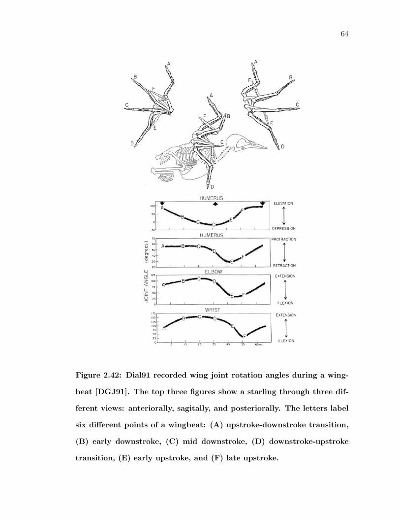
64

Figure 2.42: Dial91 recorded wing joint rotation angles during a wing-

beat [DGJ91]. The top three figures show a starling through three dif-

ferent views: anteriorally, sagitally, and posteriorally. The letters label

six different points of a wingbeat: (A) upstroke-downstroke transition,

(B) early downstroke, (C) mid downstroke, (D) downstroke-upstroke

transition, (E) early upstroke, and (F) late upstroke.

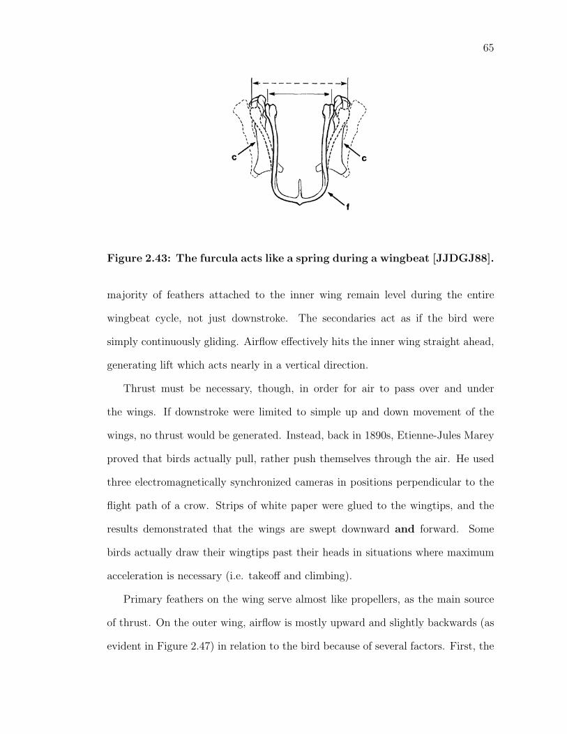
65

Figure 2.43: The furcula acts like a spring during a wingbeat [JJDGJ88].

majority of feathers attached to the inner wing remain level during the entire

wingbeat cycle, not just downstroke. The secondaries act as if the bird were

simply continuously gliding. Airflow effectively hits the inner wing straight ahead,

generating lift which acts nearly in a vertical direction.

Thrust must be necessary, though, in order for air to pass over and under

the wings. If downstroke were limited to simple up and down movement of the

wings, no thrust would be generated. Instead, back in 1890s, Etienne-Jules Marey

proved that birds actually pull, rather push themselves through the air. He used

three electromagnetically synchronized cameras in positions perpendicular to the

flight path of a crow. Strips of white paper were glued to the wingtips, and the

results demonstrated that the wings are swept downward and forward. Some

birds actually draw their wingtips past their heads in situations where maximum

acceleration is necessary (i.e. takeoff and climbing).

Primary feathers on the wing serve almost like propellers, as the main source

of thrust. On the outer wing, airflow is mostly upward and slightly backwards (as

evident in Figure 2.47) in relation to the bird because of several factors. First, the

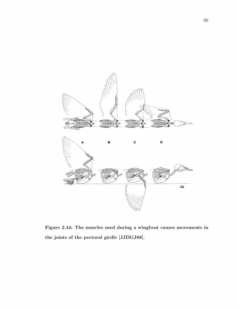
66

Figure 2.44: The muscles used during a wingbeat causes movements in

the joints of the pectoral girdle [JJDGJ88].

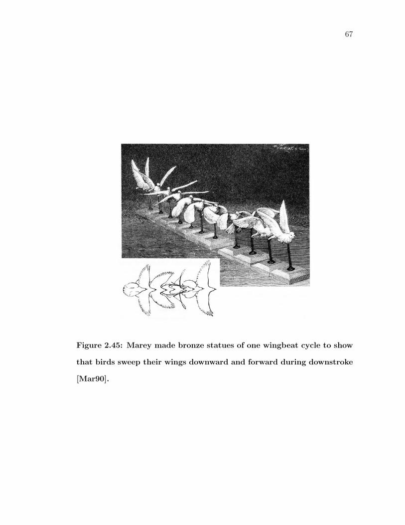
67

Figure 2.45: Marey made bronze statues of one wingbeat cycle to show

that birds sweep their wings downward and forward during downstroke

[Mar90].

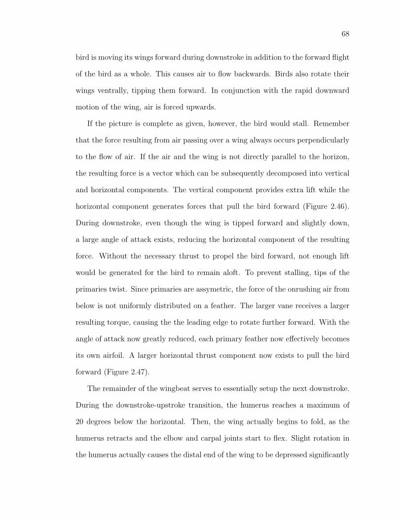
68

bird is moving its wings forward during downstroke in addition to the forward flight

of the bird as a whole. This causes air to flow backwards. Birds also rotate their

wings ventrally, tipping them forward. In conjunction with the rapid downward

motion of the wing, air is forced upwards.

If the picture is complete as given, however, the bird would stall. Remember

that the force resulting from air passing over a wing always occurs perpendicularly

to the flow of air. If the air and the wing is not directly parallel to the horizon,

the resulting force is a vector which can be subsequently decomposed into vertical

and horizontal components. The vertical component provides extra lift while the

horizontal component generates forces that pull the bird forward (Figure 2.46).

During downstroke, even though the wing is tipped forward and slightly down,

a large angle of attack exists, reducing the horizontal component of the resulting

force. Without the necessary thrust to propel the bird forward, not enough lift

would be generated for the bird to remain aloft. To prevent stalling, tips of the

primaries twist. Since primaries are assymetric, the force of the onrushing air from

below is not uniformly distributed on a feather. The larger vane receives a larger

resulting torque, causing the the leading edge to rotate further forward. With the

angle of attack now greatly reduced, each primary feather now effectively becomes

its own airfoil. A larger horizontal thrust component now exists to pull the bird

forward (Figure 2.47).

The remainder of the wingbeat serves to essentially setup the next downstroke.

During the downstroke-upstroke transition, the humerus reaches a maximum of

20 degrees below the horizontal. Then, the wing actually begins to fold, as the

humerus retracts and the elbow and carpal joints start to flex. Slight rotation in

the humerus actually causes the distal end of the wing to be depressed significantly

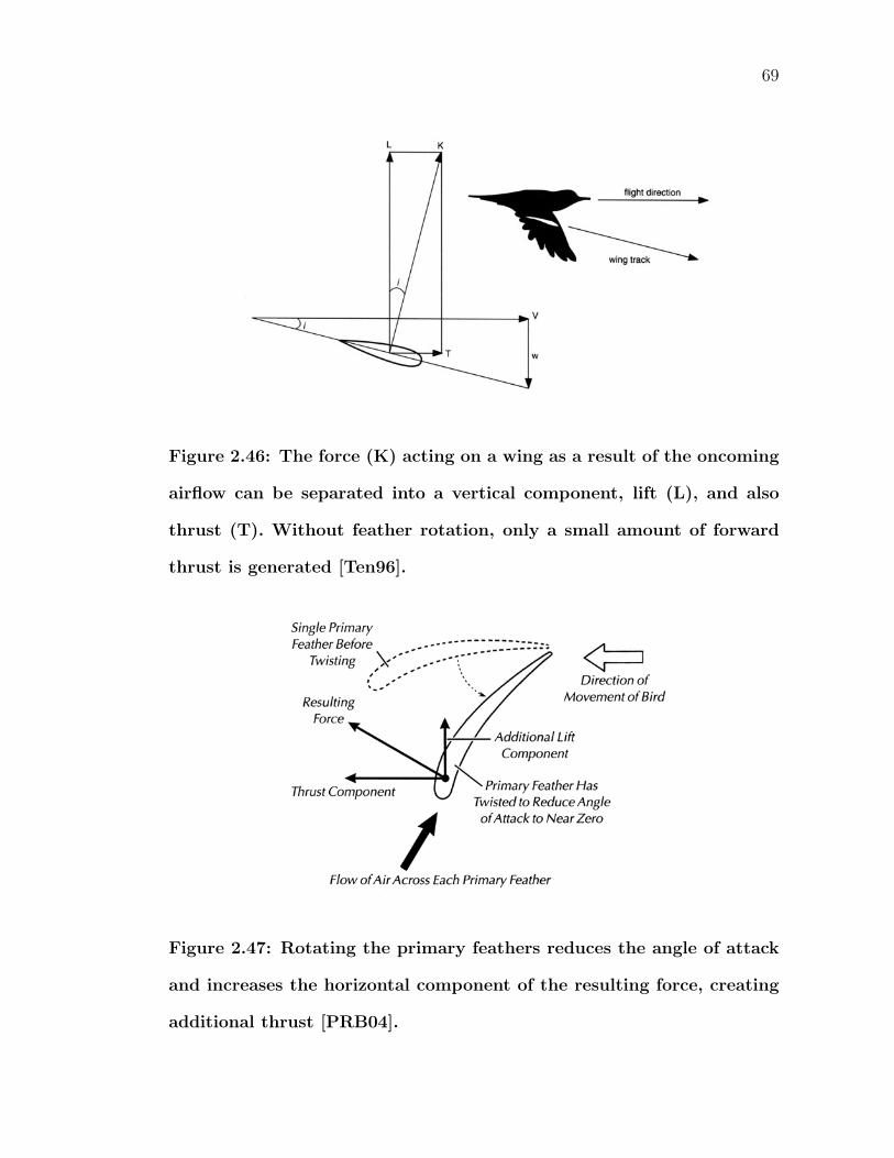
69

Figure 2.46: The force (K) acting on a wing as a result of the oncoming

airflow can be separated into a vertical component, lift (L), and also

thrust (T). Without feather rotation, only a small amount of forward

thrust is generated [Ten96].

Figure 2.47: Rotating the primary feathers reduces the angle of attack

and increases the horizontal component of the resulting force, creating

additional thrust [PRB04].

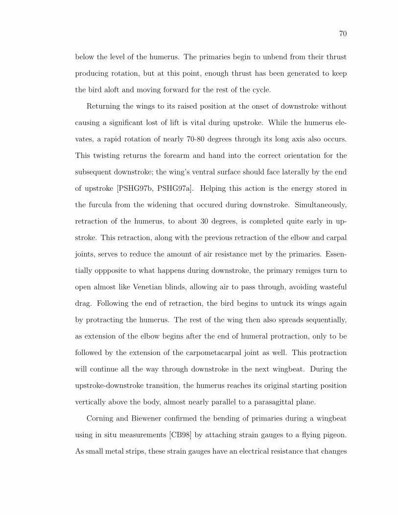
70

below the level of the humerus. The primaries begin to unbend from their thrust

producing rotation, but at this point, enough thrust has been generated to keep

the bird aloft and moving forward for the rest of the cycle.

Returning the wings to its raised position at the onset of downstroke without

causing a significant lost of lift is vital during upstroke. While the humerus ele-

vates, a rapid rotation of nearly 70-80 degrees through its long axis also occurs.

This twisting returns the forearm and hand into the correct orientation for the

subsequent downstroke; the wing’s ventral surface should face laterally by the end

of upstroke [PSHG97b, PSHG97a]. Helping this action is the energy stored in

the furcula from the widening that occured during downstroke. Simultaneously,

retraction of the humerus, to about 30 degrees, is completed quite early in up-

stroke. This retraction, along with the previous retraction of the elbow and carpal

joints, serves to reduce the amount of air resistance met by the primaries. Essen-

tially oppposite to what happens during downstroke, the primary remiges turn to

open almost like Venetian blinds, allowing air to pass through, avoiding wasteful

drag. Following the end of retraction, the bird begins to untuck its wings again

by protracting the humerus. The rest of the wing then also spreads sequentially,

as extension of the elbow begins after the end of humeral protraction, only to be

followed by the extension of the carpometacarpal joint as well. This protraction

will continue all the way through downstroke in the next wingbeat. During the

upstroke-downstroke transition, the humerus reaches its original starting position

vertically above the body, almost nearly parallel to a parasagittal plane.

Corning and Biewener confirmed the bending of primaries during a wingbeat

using in situ measurements [CB98] by attaching strain gauges to a flying pigeon.

As small metal strips, these strain gauges have an electrical resistance that changes

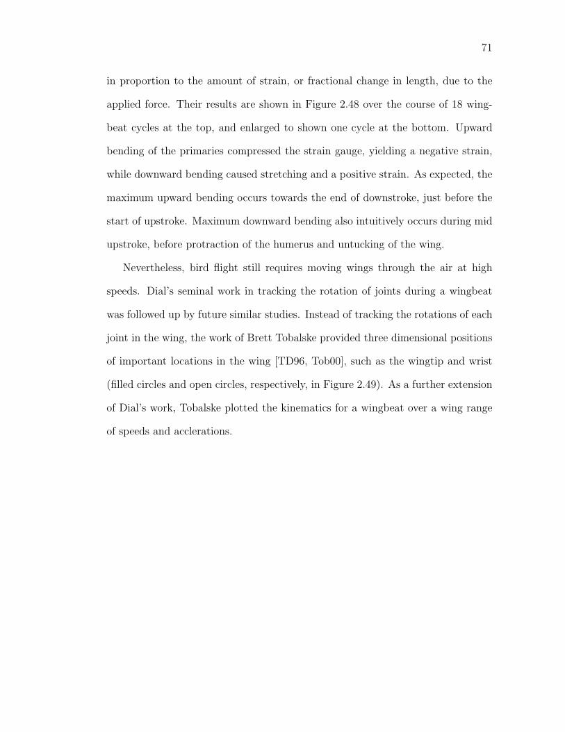
71

in proportion to the amount of strain, or fractional change in length, due to the

applied force. Their results are shown in Figure 2.48 over the course of 18 wing-

beat cycles at the top, and enlarged to shown one cycle at the bottom. Upward

bending of the primaries compressed the strain gauge, yielding a negative strain,

while downward bending caused stretching and a positive strain. As expected, the

maximum upward bending occurs towards the end of downstroke, just before the

start of upstroke. Maximum downward bending also intuitively occurs during mid

upstroke, before protraction of the humerus and untucking of the wing.

Nevertheless, bird flight still requires moving wings through the air at high

speeds. Dial’s seminal work in tracking the rotation of joints during a wingbeat

was followed up by future similar studies. Instead of tracking the rotations of each

joint in the wing, the work of Brett Tobalske provided three dimensional positions

of important locations in the wing [TD96, Tob00], such as the wingtip and wrist

(filled circles and open circles, respectively, in Figure 2.49). As a further extension

of Dial’s work, Tobalske plotted the kinematics for a wingbeat over a wing range

of speeds and acclerations.

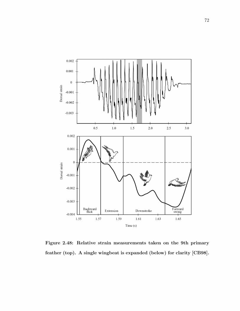
72

Figure 2.48: Relative strain measurements taken on the 9th primary

feather (top). A single wingbeat is expanded (below) for clarity [CB98].

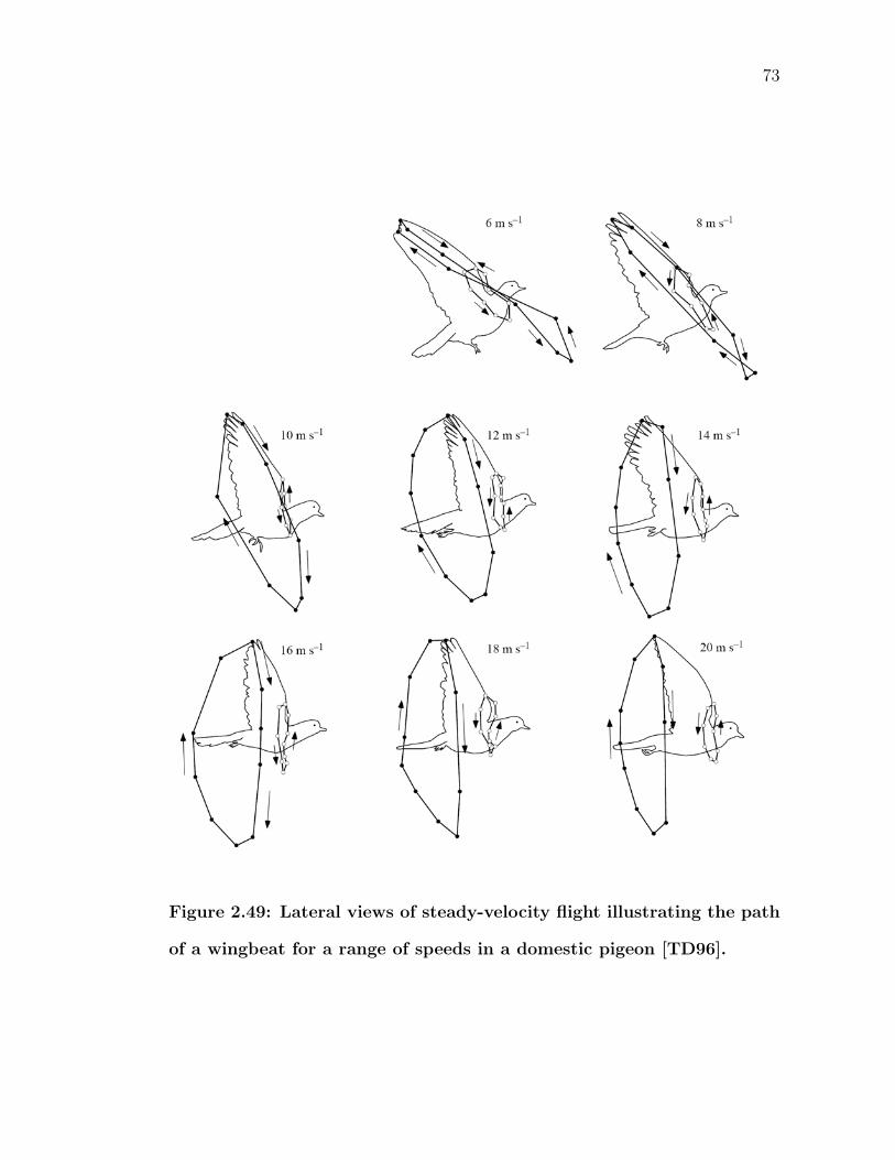
73

Figure 2.49: Lateral views of steady-velocity flight illustrating the path

of a wingbeat for a range of speeds in a domestic pigeon [TD96].

CHAPTER 3

RELATED WORKS

Previous computer graphics research relating to birds have focused on recreat-

ing individual components of avian geometry or function such as animating bird

flight or the modeling and rendering of feathers. Since the works are well seg-

mented, the following discussion has been categorized into the various parts of

the 3D production pipeline. It is important to note that no published work has

integrated these various areas together to create a scientific tool that is valuable

to ornithologists and educators alike.

Perhaps the most complete works to date are the Falcon and Margalo characters

in Sony Pictures Imageworks’ Stuart Little 2. However, as moviemakers, they set

out to meet a different set of objectives, such as expressiveness and exaggeration,

rather than scientific accuracy. In short, they needed a bird that was not necessarily

realistic, but instead believable.

3.1 Individual Feather Modeling

Most commonly, researchers have sought to construct an individual feather with

polylines, very thin triangle strips, or Bezier curves. Using these types of geome-

try, the main difficulty of a procedural feather modeling system is to concurrently

approximate both the macroscopic and microscopic levels of a feather. On a macro-

scopic level, feathers come in a variety of different types, each with its own unique

look. Microscopically, this unique look comes from a specific arrangement of the

barbs and barbules emerging from that feather’s rachis. Since this varies between

feather types, capturing the look of a specific type of feather, while maintaining

the generality to model different types of feathers, becomes challenging. Most of

74

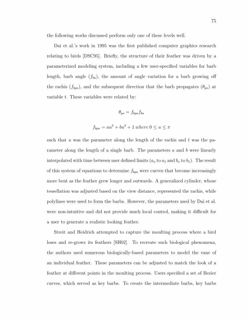
75

the following works discussed perform only one of these levels well.

Dai et al.’s work in 1995 was the first published computer graphics research

relating to birds [DSC95]. Briefly, the structure of their feather was driven by a

parameterized modeling system, including a few user-specified variables for barb

length, barb angle (fba), the amount of angle variation for a barb growing off

the rachis (fbpa), and the subsequent direction that the barb propagates (θpo) at

variable t. These variables were related by:

θpo = fbpafba

fbpa = au2 + bu2 + 1 where 0 ≤ u ≤ π

such that u was the parameter along the length of the rachis and t was the pa-

rameter along the length of a single barb. The parameters a and b were linearly

interpolated with time between user defined limits (ao to a1 and bo to b1). The result

of this system of equations to determine fbpa were curves that become increasingly

more bent as the feather grew longer and outwards. A generalized cylinder, whose

tessellation was adjusted based on the view distance, represented the rachis, while

polylines were used to form the barbs. However, the parameters used by Dai et al.

were non-intuitive and did not provide much local control, making it difficult for

a user to generate a realistic looking feather.

Streit and Heidrich attempted to capture the moulting process where a bird

loses and re-grows its feathers [SH02]. To recreate such biological phenomena,

the authors used numerous biologically-based parameters to model the vane of

an individual feather. These parameters can be adjusted to match the look of a

feather at different points in the moulting process. Users specified a set of Bezier

curves, which served as key barbs. To create the intermediate barbs, key barbs

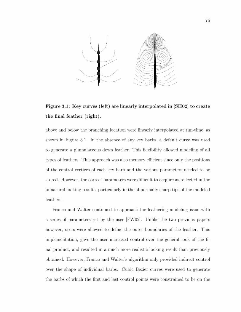
76

Figure 3.1: Key curves (left) are linearly interpolated in [SH02] to create

the final feather (right).

above and below the branching location were linearly interpolated at run-time, as

shown in Figure 3.1. In the absence of any key barbs, a default curve was used

to generate a plumulaceous down feather. This flexibility allowed modeling of all

types of feathers. This approach was also memory efficient since only the positions

of the control vertices of each key barb and the various parameters needed to be

stored. However, the correct parameters were difficult to acquire as reflected in the

unnatural looking results, particularly in the abnormally sharp tips of the modeled

feathers.

Franco and Walter continued to approach the feathering modeling issue with

a series of parameters set by the user [FW02]. Unlike the two previous papers

however, users were allowed to define the outer boundaries of the feather. This

implementation, gave the user increased control over the general look of the fi-

nal product, and resulted in a much more realistic looking result than previously

obtained. However, Franco and Walter’s algorithm only provided indirect control

over the shape of individual barbs. Cubic Bezier curves were used to generate

the barbs of which the first and last control points were constrained to lie on the

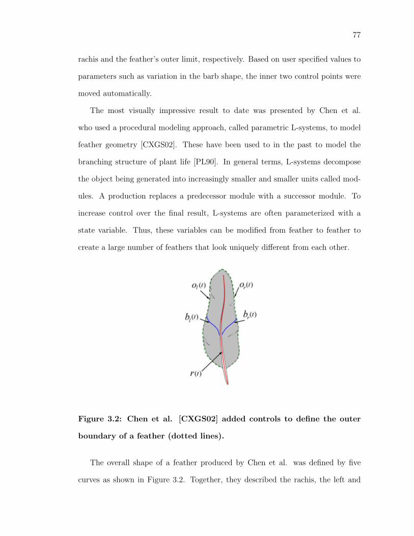
77

rachis and the feather’s outer limit, respectively. Based on user specified values to

parameters such as variation in the barb shape, the inner two control points were

moved automatically.

The most visually impressive result to date was presented by Chen et al.

who used a procedural modeling approach, called parametric L-systems, to model

feather geometry [CXGS02]. These have been used to in the past to model the

branching structure of plant life [PL90]. In general terms, L-systems decompose

the object being generated into increasingly smaller and smaller units called mod-

ules. A production replaces a predecessor module with a successor module. To

increase control over the final result, L-systems are often parameterized with a

state variable. Thus, these variables can be modified from feather to feather to

create a large number of feathers that look uniquely different from each other.

Figure 3.2: Chen et al. [CXGS02] added controls to define the outer

boundary of a feather (dotted lines).

The overall shape of a feather produced by Chen et al. was defined by five

curves as shown in Figure 3.2. Together, they described the rachis, the left and

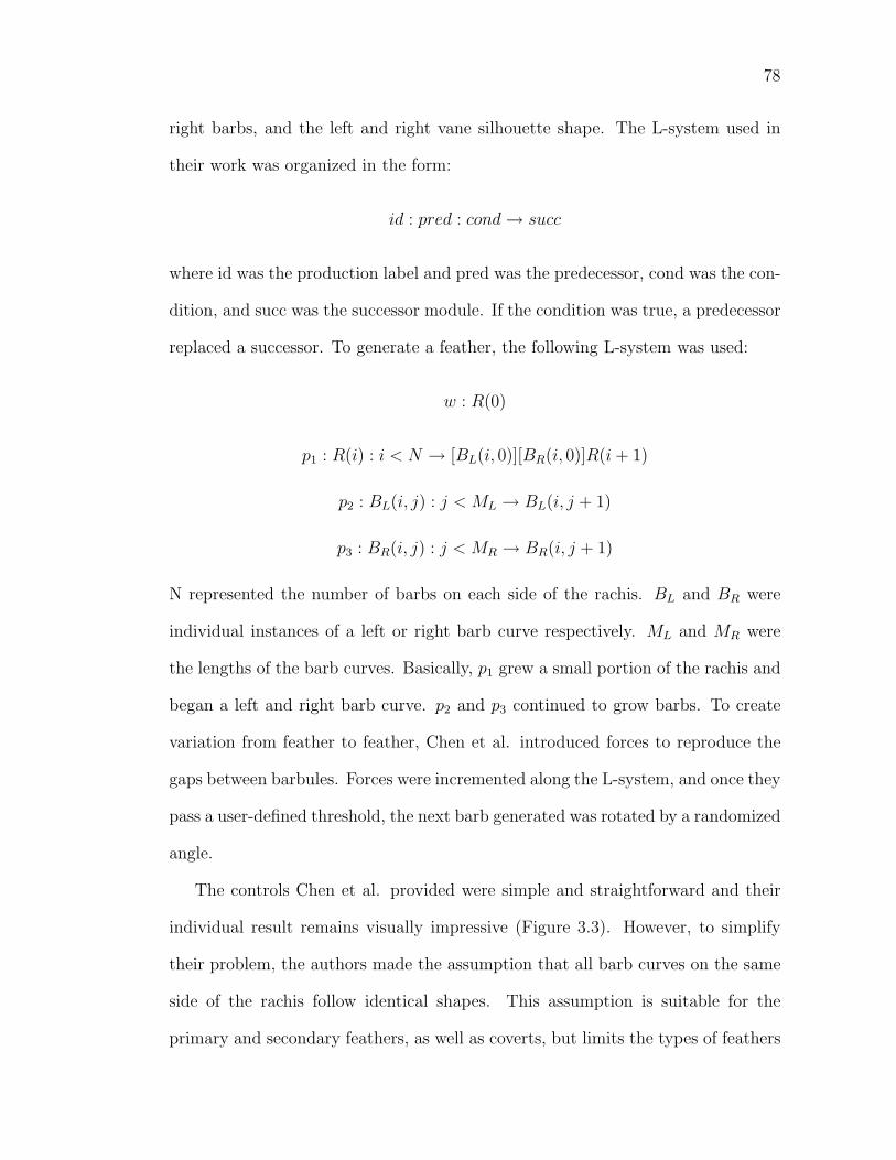
78

right barbs, and the left and right vane silhouette shape. The L-system used in

their work was organized in the form:

id : pred : cond → succ

where id was the production label and pred was the predecessor, cond was the con-

dition, and succ was the successor module. If the condition was true, a predecessor

replaced a successor. To generate a feather, the following L-system was used:

w : R(0)

p1 : R(i) : i < N → [BL(i, 0)][BR(i, 0)]R(i + 1)

p2 : BL(i, j) : j < ML → BL(i, j + 1)

p3 : BR(i, j) : j < MR → BR(i, j + 1)

N represented the number of barbs on each side of the rachis. BL and BR were

individual instances of a left or right barb curve respectively. ML and MR were

the lengths of the barb curves. Basically, p1 grew a small portion of the rachis and

began a left and right barb curve. p2 and p3 continued to grow barbs. To create

variation from feather to feather, Chen et al. introduced forces to reproduce the

gaps between barbules. Forces were incremented along the L-system, and once they

pass a user-defined threshold, the next barb generated was rotated by a randomized

angle.

The controls Chen et al. provided were simple and straightforward and their

individual result remains visually impressive (Figure 3.3). However, to simplify

their problem, the authors made the assumption that all barb curves on the same

side of the rachis follow identical shapes. This assumption is suitable for the

primary and secondary feathers, as well as coverts, but limits the types of feathers

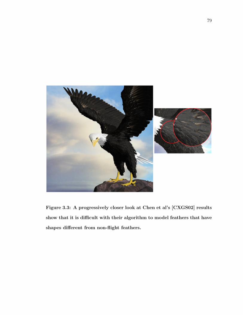
79

Figure 3.3: A progressively closer look at Chen et al’s [CXGS02] results

show that it is difficult with their algorithm to model feathers that have

shapes different from non-flight feathers.

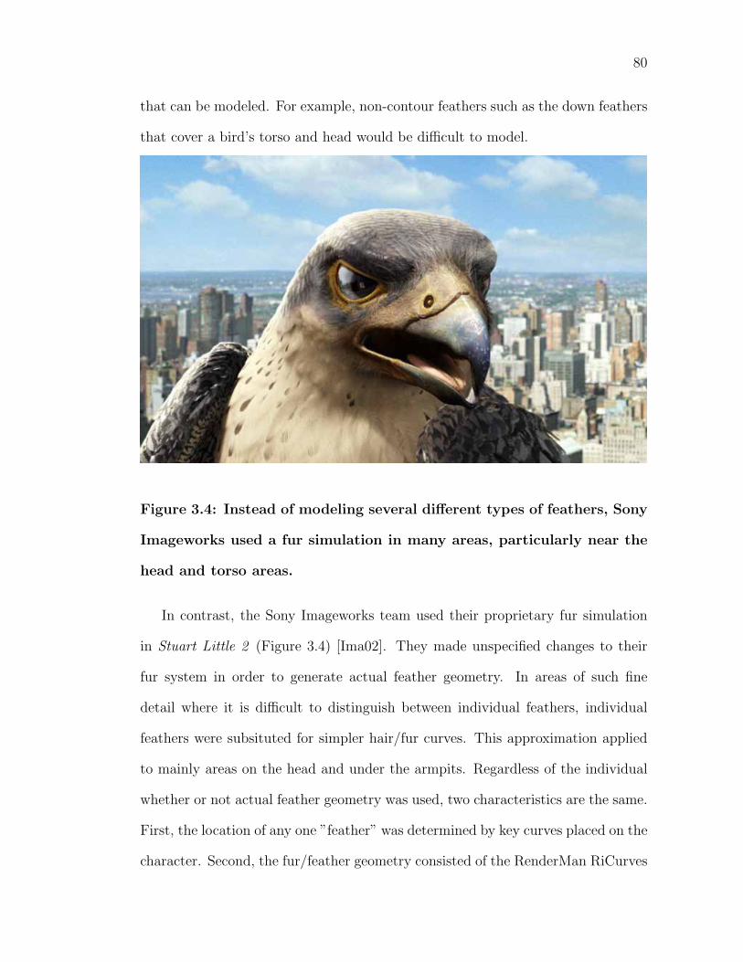
80

that can be modeled. For example, non-contour feathers such as the down feathers

that cover a bird’s torso and head would be difficult to model.

Figure 3.4: Instead of modeling several different types of feathers, Sony

Imageworks used a fur simulation in many areas, particularly near the

head and torso areas.

In contrast, the Sony Imageworks team used their proprietary fur simulation

in Stuart Little 2 (Figure 3.4) [Ima02]. They made unspecified changes to their

fur system in order to generate actual feather geometry. In areas of such fine

detail where it is difficult to distinguish between individual feathers, individual

feathers were subsituted for simpler hair/fur curves. This approximation applied

to mainly areas on the head and under the armpits. Regardless of the individual

whether or not actual feather geometry was used, two characteristics are the same.

First, the location of any one ”feather” was determined by key curves placed on the

character. Second, the fur/feather geometry consisted of the RenderMan RiCurves

81

primitive and RiProcedural dynamic shared object (DSO) feature[Bru03]. RiCurve

prims can be thought of as flat 3D ribbons with normals that, by default, are

perpendicular to the camera’s view plane. With clearly defined normals, this saves

the rendering task of having to sample where on a cylinder a light ray hits and

then determining the normal. By using DSOs to model fur/feathers that were

generated at render time, large memory expenses were saved.

3.2 Individual Feather Rendering

Generating the characteristic coloring pattern of feathers is fairly easy to do by

applying a texture map of a real feather. Because the majority of the works

used quadrilateral strips converted from Bezier splines parameterized in the [0,1]

interval, mapping coordinates are essentially obtained without any extra UV un-

wrapping. Thus, somewhat realistic looking results can be obtained without much

work. Dai et al. contributed a procedural texture generation algorithm solely for

birds in the Galliformes species.

Chen et al. took rendering a step farther by beginning to capture the unusual

spatially variant surface reflectance of feathers by using a bidirectional texture

function (BTF). A flat 2D texture poorly represents the interaction of light in any

3D object, such as the barbules at the feather’s mesostructure level, because it does

not account for the change in appearance with respect to viewing and illumination

direction. A standard 4D bidirectional reflectance distribution function (BRDF)

would be more suitable. However, since a BRDF only defines the ratio of incoming

and outgoing light at a single point, it cannot characterize the spatial variation of

reflected light in a feather. As a 6D function dependent on surface location, viewing

direction, and lighting direction, a BTF overcomes both of these shortcomings.

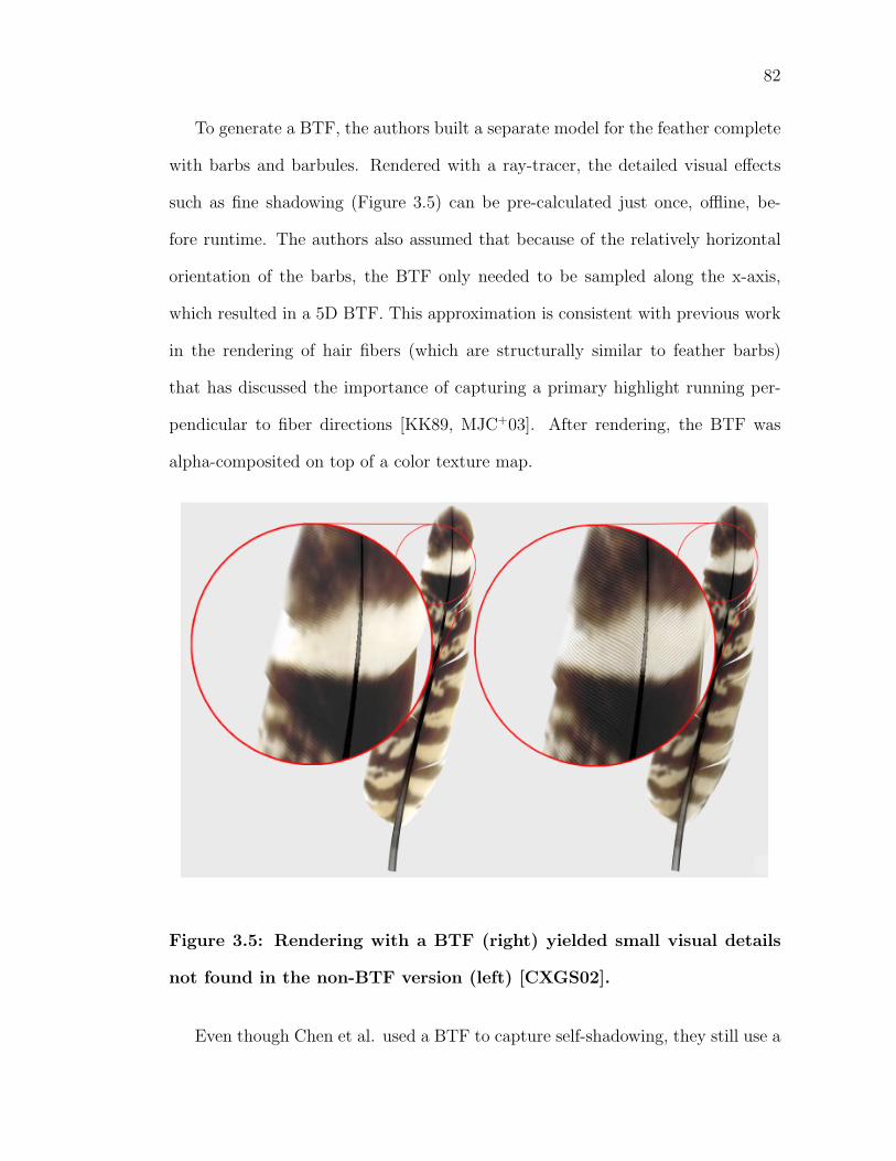
82

To generate a BTF, the authors built a separate model for the feather complete

with barbs and barbules. Rendered with a ray-tracer, the detailed visual effects

such as fine shadowing (Figure 3.5) can be pre-calculated just once, offline, be-

fore runtime. The authors also assumed that because of the relatively horizontal

orientation of the barbs, the BTF only needed to be sampled along the x-axis,

which resulted in a 5D BTF. This approximation is consistent with previous work

in the rendering of hair fibers (which are structurally similar to feather barbs)

that has discussed the importance of capturing a primary highlight running per-

pendicular to fiber directions [KK89, MJC+03]. After rendering, the BTF was

alpha-composited on top of a color texture map.

Figure 3.5: Rendering with a BTF (right) yielded small visual details

not found in the non-BTF version (left) [CXGS02].

Even though Chen et al. used a BTF to capture self-shadowing, they still use a

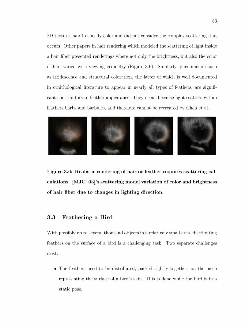
83

2D texture map to specify color and did not consider the complex scattering that

occurs. Other papers in hair rendering which modeled the scattering of light inside

a hair fiber presented renderings where not only the brightness, but also the color

of hair varied with viewing geometry (Figure 3.6). Similarly, phenomenon such

as irridescence and structural coloration, the latter of which is well documented

in ornithological literature to appear in nearly all types of feathers, are signifi-

cant contributors to feather appearance. They occur because light scatters within

feathers barbs and barbules, and therefore cannot be recreated by Chen et al..

Figure 3.6: Realistic rendering of hair or feather requires scattering cal-

culations. [MJC+03]’s scattering model variation of color and brightness

of hair fiber due to changes in lighting direction.

3.3 Feathering a Bird

With possibly up to several thousand objects in a relatively small area, distributing

feathers on the surface of a bird is a challenging task. Two separate challenges

exist:

• The feathers need to be distributed, packed tightly together, on the mesh

representing the surface of a bird’s skin. This is done while the bird is in a

static pose.

84

• During animation of the bird, the feathers are animated without having them

intersect each other or the skin.

Obviously, placing every single feather on a bird becomes a tedious task. This

problem was solved in detail by both Chen et al. and Sony Imageworks. However,

their approaches are slightly different because of their intended usages. Chen et

al. generated an image of a bird in a static pose with high computing costs. On

the other hand, Sony Imageworks needed a solution that was controllable and not

terribly time consuming given the tight time budgets associated with animating a

feature film. Much detail of their algorithms remain unpublished. Unless explicitly

stated, the descriptions of the Imageworks feathering system that follows were

based on their fur simulation, from which the feathering system originated.

Chen et al. and Imageworks started off similarly. First, they let the user

manually specify key feathers and their properties, including orientation, growing

direction, and the amount of twist. These key feathers lay on the vertices of

the bird’s skin mesh. To add more control, Sony used painted texture maps to

specify these properties. Both then ran separate algorithms, Turk’s algorithm from

[Tur92] and the repulsive force mechanism from [WH94], respectively, to sample

and distribute the positions of key feathers on the skin. These algorithms were

modified from their original form so that feathers can be distributed non-uniformly.

Specifically, Chen et al. modified Turk’s algorithm so that vertex density can be

dependent on feather size, which was interpolated using Gaussian radial basis

functions. As a result, areas that have smaller feathers were more populated.

However, Chen et al’s algorithm re-tiled the skin mesh, possibly destroying the

topology that was optimized for easier animation. No details were given as to

whether or not Imageworks’ algorithm does the same, though the topology is

85

assumed to be left untouched.

The next step was to fill in the gaps between the key curves/feathers using

an interpolation routine. Once interpolation generated the rest of the feathers,

manually editing the key feathers modified the entire coat.

The Gaussian radial basis functions are commonly used to provide weights

for multi-dimensional scattered data interpolation. The Gaussian family of radial

basis functions decrease in value rapidly away from an origin. In Chen et al.’s case

of feathering a bird, the distance between data points was the distance (calculated

using Dijkstra’s shortest path algorithm) between key feathers. Significantly less

influence was then given to a key feather that lay further away than one nearby.

Imageworks decomposed their procedure into static, frame-independent oper-

ations and calculations that need to be run each frame [Bru03]. An “instancer”

handled the former, while an “interpolator” took care of the latter. The instancer

received the key curves and attribute texture maps as input and then generated

the following three properties for each of the final hairs in the rendered image:

• An interpolated hair’s position

• Three vertices of the triangle defining where an interpolated hair lies

• Weights for each of these three key curves.

The position of each final hair, in local model space, was determined by a density

attribute that specifies the number of hairs per square unit area. Two-dimensional

Delaunay triangulation broke the NURBS patches into triangles. By looking up

the triangle that the hair of interest falls into, the three key curves needed for

interpolation were determined. Barycentric coordinates were used to generate

weights for each of these key curves.

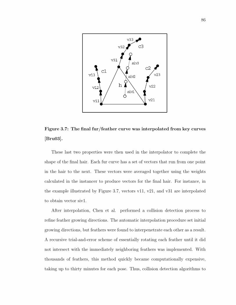
86

Figure 3.7: The final fur/feather curve was interpolated from key curves

[Bru03].

These last two properties were then used in the interpolator to complete the

shape of the final hair. Each fur curve has a set of vectors that run from one point

in the hair to the next. These vectors were averaged together using the weights

calculated in the instancer to produce vectors for the final hair. For instance, in

the example illustrated by Figure 3.7, vectors v11, v21, and v31 are interpolated

to obtain vector siv1.

After interpolation, Chen et al. performed a collision detection process to

refine feather growing directions. The automatic interpolation procedure set initial

growing directions, but feathers were found to interpenetrate each other as a result.

A recursive trial-and-error scheme of essentially rotating each feather until it did

not intersect with the immediately neighboring feathers was implemented. With

thousands of feathers, this method quickly became computationally expensive,

taking up to thirty minutes for each pose. Thus, collision detection algorithms to

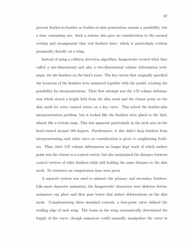
87

prevent feather-to-feather or feather-to-skin penetration remain a possibility, but

a time consuming one. Such a scheme also gave no consideration to the natural

overlap and arrangement that real feathers have, which is particularly evident

proximally/distally on a wing.

Instead of using a collision detection algorithm, Imageworks created what they

called a one-dimensional and also a two-dimensional volume deformation tech-

nique, for the feathers on the bird’s torso. The key curves that originally specified

the locations of the feathers were animated together with the model, creating the

possibility for interpenetration. Their first attempt was the 1-D volume deforma-

tion which stored a height field from the skin mesh and the closest point on the

skin mesh for every control vertex on a key curve. This solved the feather-skin

interpenetration problem, but it looked like the feathers were glued to the bird,

almost like a texture map. This was apparent particularly in the neck area as the

head turned around 180 degrees. Furthermore, it also didn’t keep feathers from

interpenetrating each other since no consideration is given to neighboring feath-

ers. Thus, their 2-D volume deformation no longer kept track of which surface

point was the closest to a control vertex, but also maintained the distance between

control vertices of other feathers while still holding the same distance to the skin

mesh. No statistics on computation time were given.

A separate system was used to animate the primary and secondary feathers.

Like most character animation, the Imageworks’ characters were skeleton driven:

animators can place and then pose bones that induce deformations on the skin

mesh. Complementing these standard controls, a four-point curve defined the

trailing edge of each wing. The bones in the wing automatically determined the

length of the curve, though animators could manually manipulate the curve in

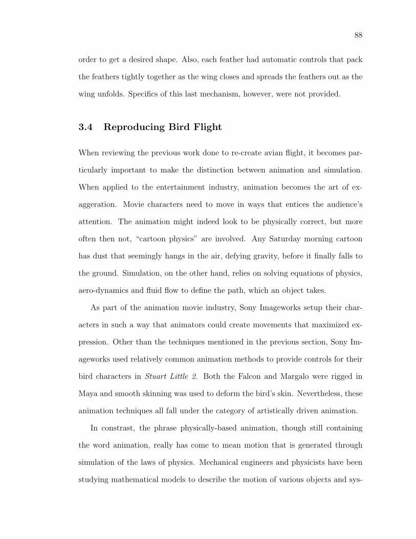
88

order to get a desired shape. Also, each feather had automatic controls that pack

the feathers tightly together as the wing closes and spreads the feathers out as the

wing unfolds. Specifics of this last mechanism, however, were not provided.

3.4 Reproducing Bird Flight

When reviewing the previous work done to re-create avian flight, it becomes par-

ticularly important to make the distinction between animation and simulation.

When applied to the entertainment industry, animation becomes the art of ex-

aggeration. Movie characters need to move in ways that entices the audience’s

attention. The animation might indeed look to be physically correct, but more

often then not, “cartoon physics” are involved. Any Saturday morning cartoon

has dust that seemingly hangs in the air, defying gravity, before it finally falls to

the ground. Simulation, on the other hand, relies on solving equations of physics,

aero-dynamics and fluid flow to define the path, which an object takes.

As part of the animation movie industry, Sony Imageworks setup their char-

acters in such a way that animators could create movements that maximized ex-

pression. Other than the techniques mentioned in the previous section, Sony Im-

ageworks used relatively common animation methods to provide controls for their

bird characters in Stuart Little 2. Both the Falcon and Margalo were rigged in

Maya and smooth skinning was used to deform the bird’s skin. Nevertheless, these

animation techniques all fall under the category of artistically driven animation.

In constrast, the phrase physically-based animation, though still containing

the word animation, really has come to mean motion that is generated through

simulation of the laws of physics. Mechanical engineers and physicists have been

studying mathematical models to describe the motion of various objects and sys-

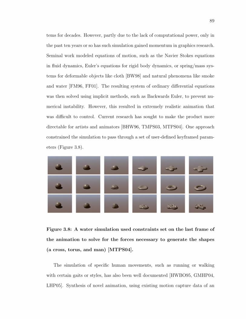
89

tems for decades. However, partly due to the lack of computational power, only in

the past ten years or so has such simulation gained momentum in graphics research.

Seminal work modeled equations of motion, such as the Navier Stokes equations

in fluid dynamics, Euler’s equations for rigid body dynamics, or spring/mass sys-

tems for deformable objects like cloth [BW98] and natural phenomena like smoke

and water [FM96, FF01]. The resulting system of ordinary differential equations

was then solved using implicit methods, such as Backwards Euler, to prevent nu-

merical instability. However, this resulted in extremely realistic animation that

was difficult to control. Current research has sought to make the product more

directable for artists and animators [BHW96, TMPS03, MTPS04]. One approach

constrained the simulation to pass through a set of user-defined keyframed param-

eters (Figure 3.8).

Figure 3.8: A water simulation used constraints set on the last frame of

the animation to solve for the forces necessary to generate the shapes

(a cross, torus, and man) [MTPS04].

The simulation of specific human movements, such as running or walking

with certain gaits or styles, has also been well documented [HWBO95, GMHP04,

LHP05]. Synthesis of novel animation, using existing motion capture data of an

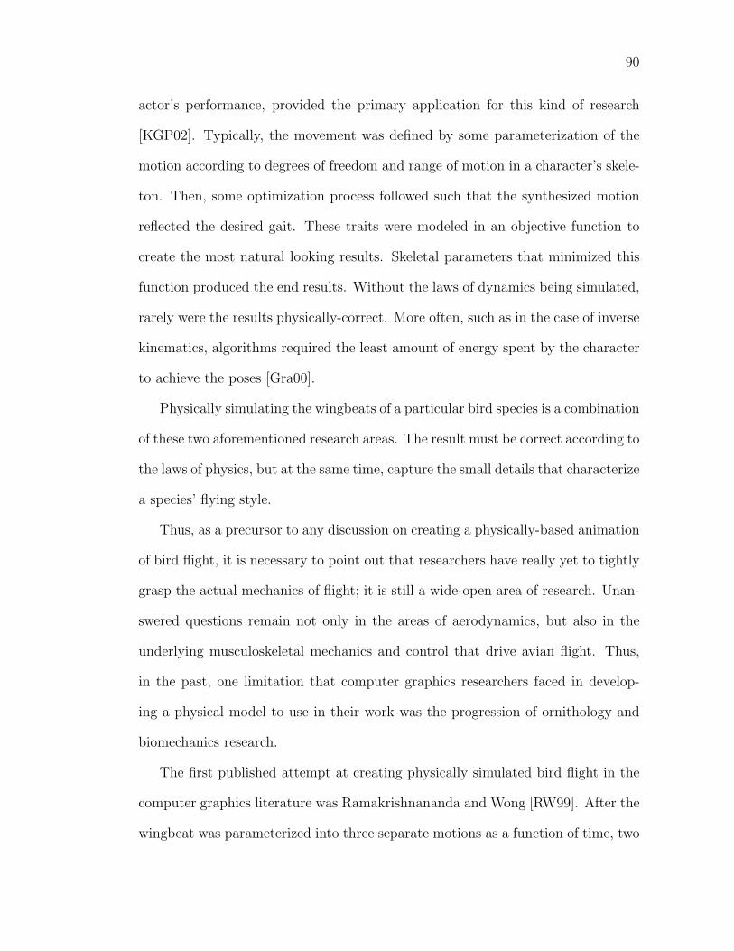
90

actor’s performance, provided the primary application for this kind of research

[KGP02]. Typically, the movement was defined by some parameterization of the

motion according to degrees of freedom and range of motion in a character’s skele-

ton. Then, some optimization process followed such that the synthesized motion

reflected the desired gait. These traits were modeled in an objective function to

create the most natural looking results. Skeletal parameters that minimized this

function produced the end results. Without the laws of dynamics being simulated,

rarely were the results physically-correct. More often, such as in the case of inverse

kinematics, algorithms required the least amount of energy spent by the character

to achieve the poses [Gra00].

Physically simulating the wingbeats of a particular bird species is a combination

of these two aforementioned research areas. The result must be correct according to

the laws of physics, but at the same time, capture the small details that characterize

a species’ flying style.

Thus, as a precursor to any discussion on creating a physically-based animation

of bird flight, it is necessary to point out that researchers have really yet to tightly

grasp the actual mechanics of flight; it is still a wide-open area of research. Unan-

swered questions remain not only in the areas of aerodynamics, but also in the

underlying musculoskeletal mechanics and control that drive avian flight. Thus,

in the past, one limitation that computer graphics researchers faced in develop-

ing a physical model to use in their work was the progression of ornithology and

biomechanics research.

The first published attempt at creating physically simulated bird flight in the

computer graphics literature was Ramakrishnananda and Wong [RW99]. After the

wingbeat was parameterized into three separate motions as a function of time, two

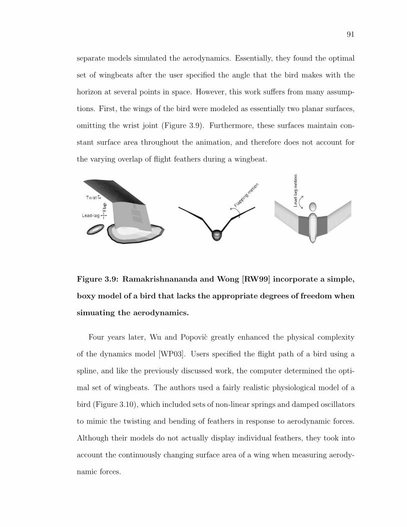
91

separate models simulated the aerodynamics. Essentially, they found the optimal

set of wingbeats after the user specified the angle that the bird makes with the

horizon at several points in space. However, this work suffers from many assump-

tions. First, the wings of the bird were modeled as essentially two planar surfaces,

omitting the wrist joint (Figure 3.9). Furthermore, these surfaces maintain con-

stant surface area throughout the animation, and therefore does not account for

the varying overlap of flight feathers during a wingbeat.

Figure 3.9: Ramakrishnananda and Wong [RW99] incorporate a simple,

boxy model of a bird that lacks the appropriate degrees of freedom when

simuating the aerodynamics.

Four years later, Wu and Popovic greatly enhanced the physical complexity

of the dynamics model [WP03]. Users specified the flight path of a bird using a

spline, and like the previously discussed work, the computer determined the opti-

mal set of wingbeats. The authors used a fairly realistic physiological model of a

bird (Figure 3.10), which included sets of non-linear springs and damped oscillators

to mimic the twisting and bending of feathers in response to aerodynamic forces.

Although their models do not actually display individual feathers, they took into

account the continuously changing surface area of a wing when measuring aerody-

namic forces.

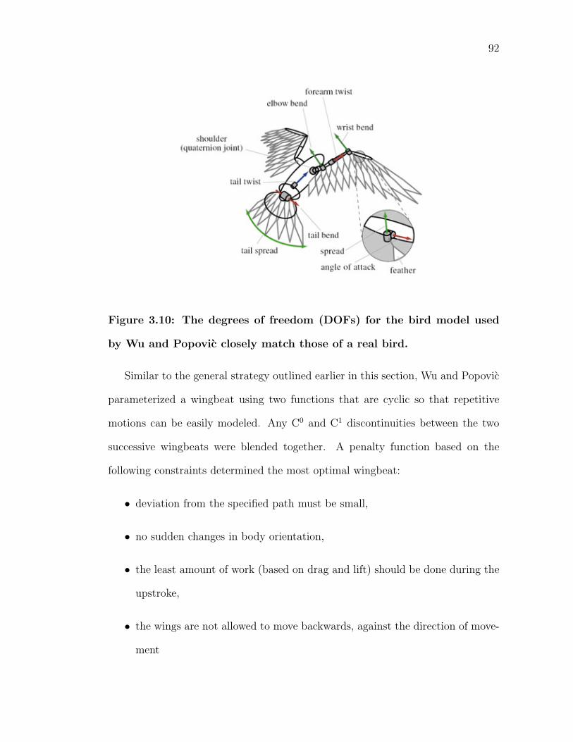
92

Figure 3.10: The degrees of freedom (DOFs) for the bird model used

by Wu and Popovic closely match those of a real bird.

Similar to the general strategy outlined earlier in this section, Wu and Popovic

parameterized a wingbeat using two functions that are cyclic so that repetitive

motions can be easily modeled. Any C0 and C1 discontinuities between the two

successive wingbeats were blended together. A penalty function based on the

following constraints determined the most optimal wingbeat:

• deviation from the specified path must be small,

• no sudden changes in body orientation,

• the least amount of work (based on drag and lift) should be done during the

upstroke,

• the wings are not allowed to move backwards, against the direction of move-

ment

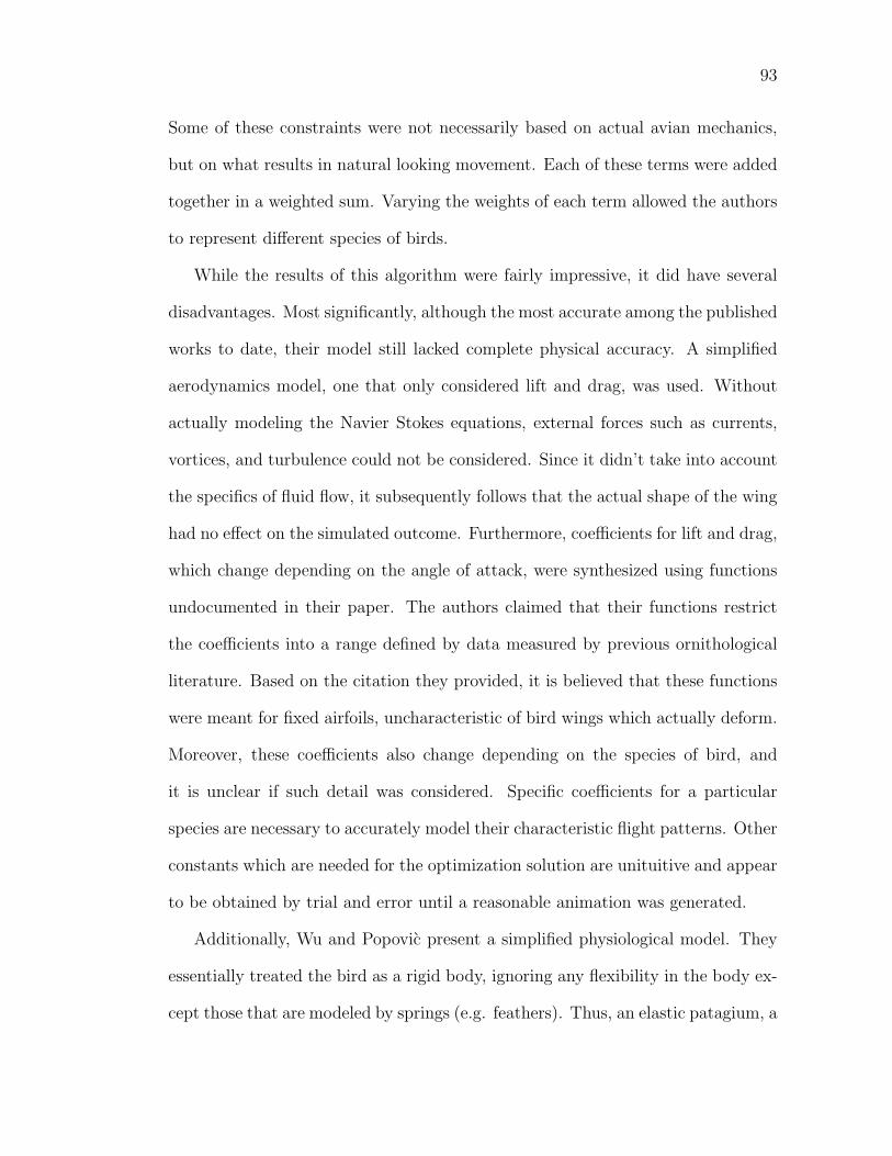
93

Some of these constraints were not necessarily based on actual avian mechanics,

but on what results in natural looking movement. Each of these terms were added

together in a weighted sum. Varying the weights of each term allowed the authors

to represent different species of birds.

While the results of this algorithm were fairly impressive, it did have several

disadvantages. Most significantly, although the most accurate among the published

works to date, their model still lacked complete physical accuracy. A simplified

aerodynamics model, one that only considered lift and drag, was used. Without

actually modeling the Navier Stokes equations, external forces such as currents,

vortices, and turbulence could not be considered. Since it didn’t take into account

the specifics of fluid flow, it subsequently follows that the actual shape of the wing

had no effect on the simulated outcome. Furthermore, coefficients for lift and drag,

which change depending on the angle of attack, were synthesized using functions

undocumented in their paper. The authors claimed that their functions restrict

the coefficients into a range defined by data measured by previous ornithological

literature. Based on the citation they provided, it is believed that these functions

were meant for fixed airfoils, uncharacteristic of bird wings which actually deform.

Moreover, these coefficients also change depending on the species of bird, and

it is unclear if such detail was considered. Specific coefficients for a particular

species are necessary to accurately model their characteristic flight patterns. Other

constants which are needed for the optimization solution are unituitive and appear

to be obtained by trial and error until a reasonable animation was generated.

Additionally, Wu and Popovic present a simplified physiological model. They

essentially treated the bird as a rigid body, ignoring any flexibility in the body ex-

cept those that are modeled by springs (e.g. feathers). Thus, an elastic patagium, a

94

significant contributor of lift for a real bird, was not present to fill in the triangular

gap between between the shoulder and wrist joints, as evidenced in Figure 3.10.

Lastly, the simulation remained computationally expensive (in the magnitude of

hours for a few seconds of animation). Each wingbeat went through 1000 iterations

in a simulated annealing before settling upon the most optimal values.

CHAPTER 4

RECONSTRUCTION AND MODELING OF THE IVORY-BILLED

WOODPECKER

Our goal is to create a physiologically correct animation of the Ivory-Billed

Woodpecker which closely mimics the actual flying behavior of the bird. To ap-

proximate the flight simulation using standard animation technology, it is necessary

to first obtain a precise geometric description of the Ivory-Billed Woodpecker. This

geometric description must then be put into an animatable model so its motions

and deformations can be accurately controlled. In attempting to get an exact

replica of the geometry it was necessary to divide our task into three steps.

The first step was to use computerized tomography to obtain a volumetric

description of the bird’s geometry and skeletal system. The second step was to

create a polygonal surface description, the reference model, of the bird’s geometry

to be used as a template for the creation of the animatable model. The third step,

the creation of the animatable model, requires carefully constructing an accurate

skin mesh that is better suited for animation purposes. This chapter describes

the three steps we used to create our animatable model. The addition of feathers

which are such a large part of the visualization of this bird is covered in Chapter 6.

4.1 Computerized Tomography Scanning

Various computer imaging technologies can capture an object’s geometry. For

example, laser range scanning devices are commonly used in the entertainment

industry, but are restricted to recording only surface details. These methods are

frequently handicapped by occlusion problems, limiting the “capturable” geometry

to only areas where the laser can reach the surface. However, a vital part of our

95

96

project is to obtain the dimensions and relative proportions of both the Ivory-

Billed’s skeleton and the Ivory-Billed’s skin, so these methods do not meet our

needs.

In contrast, doctors and radiologists frequently use modern medical imaging

technologies to uncover subsurface details hidden to the eye. Depending on the

object of interest’s tissue composition, the appropriate imaging technique can be

selected. Projection radiography, otherwise known as the standard x-ray, has es-

tablished itself as a powerful, cost-effective standard to detect bone injuries for

decades. However, as only a two-dimensional projection of a three dimensional

object coupled with its inability to image soft tissue, standard x-ray approaches

fall short of being a suitable method for capturing the required geometrical data.

More appropriate are the recent advances in tomography, which capture data of a

single slice through an entire object. A collection of these slices provides enough

volumetric data to record and display the shape of the specimen.

A computerized tomography (CT) scanner works similarly to a regular x-ray

machine. Small doses of x-ray radiation are passed through the body, and like

x-rays, the radiation is absorbed at differing rates, which are directly proportional

to a material’s radiographic density. Measured in terms of Housefield units, these

values can span a range from -1024 HU to +3071 HU. For example, room air is

-1000 HU, while water is 0 HU. Organic tissue frequently presents higher values.

Soft tissue lies in the +40-80 HU range and bone can reach as high as +1000 HU

(Figure 4.1).

In contrast to x-rays which are captured on special film, an array of detectors

measures the amount of radiation that has passed through the body. The emitter

and detector in a CT scanner lie on opposite sides of one another in a rotating

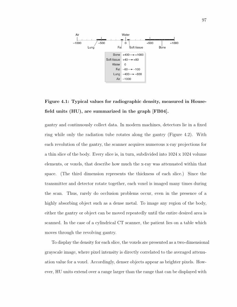
97

Figure 4.1: Typical values for radiographic density, measured in House-

field units (HU), are summarized in the graph [FB04].

gantry and continuously collect data. In modern machines, detectors lie in a fixed

ring while only the radiation tube rotates along the gantry (Figure 4.2). With

each revolution of the gantry, the scanner acquires numerous x-ray projections for

a thin slice of the body. Every slice is, in turn, subdivided into 1024 x 1024 volume

elements, or voxels, that describe how much the x-ray was attenuated within that

space. (The third dimension represents the thickness of each slice.) Since the

transmitter and detector rotate together, each voxel is imaged many times during

the scan. Thus, rarely do occlusion problems occur, even in the presence of a

highly absorbing object such as a dense metal. To image any region of the body,

either the gantry or object can be moved repeatedly until the entire desired area is

scanned. In the case of a cylindrical CT scanner, the patient lies on a table which

moves through the revolving gantry.

To display the density for each slice, the voxels are presented as a two-dimensional

grayscale image, where pixel intensity is directly correlated to the averaged attenu-

ation value for a voxel. Accordingly, denser objects appear as brighter pixels. How-

ever, HU units extend over a range larger than the range that can be displayed with

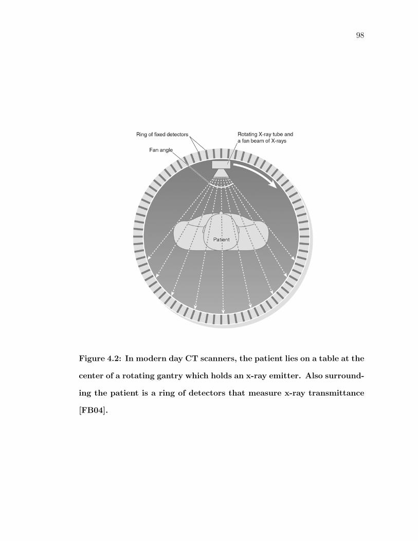
98

Figure 4.2: In modern day CT scanners, the patient lies on a table at the

center of a rotating gantry which holds an x-ray emitter. Also surround-

ing the patient is a ring of detectors that measure x-ray transmittance

[FB04].

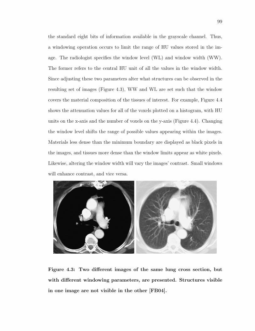
99

the standard eight bits of information available in the grayscale channel. Thus,

a windowing operation occurs to limit the range of HU values stored in the im-

age. The radiologist specifies the window level (WL) and window width (WW).

The former refers to the central HU unit of all the values in the window width.

Since adjusting these two parameters alter what structures can be observed in the

resulting set of images (Figure 4.3), WW and WL are set such that the window

covers the material composition of the tissues of interest. For example, Figure 4.4

shows the attenuation values for all of the voxels plotted on a histogram, with HU

units on the x-axis and the number of voxels on the y-axis (Figure 4.4). Changing

the window level shifts the range of possible values appearing within the images.

Materials less dense than the minimum boundary are displayed as black pixels in

the images, and tissues more dense than the window limits appear as white pixels.

Likewise, altering the window width will vary the images’ contrast. Small windows

will enhance contrast, and vice versa.

Figure 4.3: Two different images of the same lung cross section, but

with different windowing parameters, are presented. Structures visible

in one image are not visible in the other [FB04].

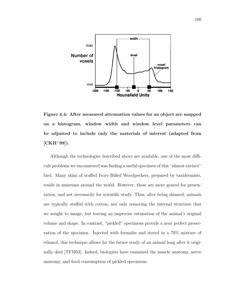
100

Figure 4.4: After measured attenuation values for an object are mapped

on a histogram, window width and window level parameters can

be adjusted to include only the materials of interest (adapted from

[CKH+99]).

Although the technologies described above are available, one of the most diffi-

cult problems we encountered was finding a useful specimen of this “almost extinct”

bird. Many skins of stuffed Ivory-Billed Woodpeckers, prepared by taxidermists,

reside in museums around the world. However, these are more geared for presen-

tation, and not necessarily for scientific study. Thus, after being skinned, animals

are typically stuffed with cotton, not only removing the internal structure that

we sought to image, but leaving an imprecise estimation of the animal’s original

volume and shape. In contrast, “pickled” specimens provide a near perfect preser-

vation of the specimen. Injected with formalin and stored in a 70% mixture of

ethanol, this technique allows for the future study of an animal long after it origi-

nally died [TFM03]. Indeed, biologists have examined the muscle anatomy, nerve

anatomy, and food consumption of pickled specimens.

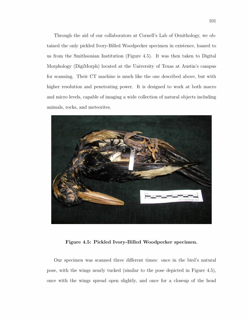
101

Through the aid of our collaborators at Cornell’s Lab of Ornithology, we ob-

tained the only pickled Ivory-Billed Woodpecker specimen in existence, loaned to

us from the Smithsonian Institution (Figure 4.5). It was then taken to Digital

Morphology (DigiMorph) located at the University of Texas at Austin’s campus

for scanning. Their CT machine is much like the one described above, but with

higher resolution and penetrating power. It is designed to work at both macro

and micro levels, capable of imaging a wide collection of natural objects including

animals, rocks, and meteorites.

Figure 4.5: Pickled Ivory-Billed Woodpecker specimen.

Our specimen was scanned three different times: once in the bird’s natural

pose, with the wings nearly tucked (similar to the pose depicted in Figure 4.5),

once with the wings spread open slightly, and once for a closeup of the head

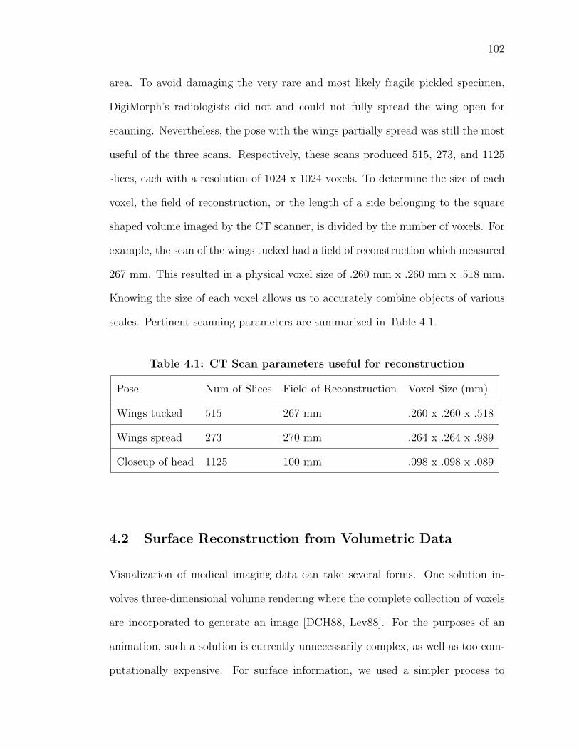
102

area. To avoid damaging the very rare and most likely fragile pickled specimen,

DigiMorph’s radiologists did not and could not fully spread the wing open for

scanning. Nevertheless, the pose with the wings partially spread was still the most

useful of the three scans. Respectively, these scans produced 515, 273, and 1125

slices, each with a resolution of 1024 x 1024 voxels. To determine the size of each

voxel, the field of reconstruction, or the length of a side belonging to the square

shaped volume imaged by the CT scanner, is divided by the number of voxels. For

example, the scan of the wings tucked had a field of reconstruction which measured

267 mm. This resulted in a physical voxel size of .260 mm x .260 mm x .518 mm.

Knowing the size of each voxel allows us to accurately combine objects of various

scales. Pertinent scanning parameters are summarized in Table 4.1.

Table 4.1: CT Scan parameters useful for reconstruction

Pose Num of Slices Field of Reconstruction Voxel Size (mm)

Wings tucked 515 267 mm .260 x .260 x .518

Wings spread 273 270 mm .264 x .264 x .989

Closeup of head 1125 100 mm .098 x .098 x .089

4.2 Surface Reconstruction from Volumetric Data

Visualization of medical imaging data can take several forms. One solution in-

volves three-dimensional volume rendering where the complete collection of voxels

are incorporated to generate an image [DCH88, Lev88]. For the purposes of an

animation, such a solution is currently unnecessarily complex, as well as too com-

putationally expensive. For surface information, we used a simpler process to

103

extract the geometry. Dating back to at least the 1980s, this kind of reconstruc-

tion was among the first applications of computer graphics to medical data sets

[LC87].

Slices from the volumetric scan data were brought into Template Graphics’

Amira, a high end visualization software for medical imaging. Since we were inter-

ested in obtaining the skin and skeletal structure, our first step was to mark these

features in the series of images. As shown in Figure 4.2, most biological materials

are radiologically dense, and therefore lie at the higher end of the intensity range.

Thus, one could correctly conclude that in a typical slice of a CT scan, an animal’s

body would appear as a continuous section of bright pixels surrounded by a region

of dark pixels representing air.

Thresholding uses this assumption to automatically segment each slice and

define isocontours [SSAC88, SFF91]. By essentially partitioning together regions

of pixels in an image with similar properties, the operation itself is similar to edge

finding operations in computer vision. Various criteria such as hue can be used,

but with CT imaging, pixels are usually sorted according to intensity. Given a

user specified value, thresholding algorithms delineate between the interior and

exterior of our intended surface within each slice; pixels brighter than the specified

value are inside while darker pixels lie on the surface’s exterior. These methods

examine an image by evaluating all of the pixels in a slice one at a time. All

pixels are either assigned a value of one if they are inside the object and zero if

they belong to the background. The result is essentially a binary image. However,

noise from the imaging device itself often complicates matters by introducing small

fluctuations in pixel intensities, even though they belong to the same object. As

a solution, supplementary research has introduced several improvements to the

104

basic algorithm. Instead of considering a pixel on an individual basis, one common

approach makes thresholding decisions by examing the intensities of neighboring

pixels as well, and then applying various statistical analyses to produce a smooth

contour [SM00].

In the example illustrated by Figure 4.6, Amira’s thresholding algorithms gen-

erated an outline (shown in yellow) of the Ivory-Billed Woodpecker’s skin surface.

Using a different, higher threshold, the same procedure was used to generate con-

tours for the Ivory-Billed’s skeleton.

One of the commonly cited drawbacks of surface rendering medical imaging

datasets, as opposed to volume rendering, is its inability to segment individual

structures that do not have well-differentiated surfaces. Structures that have sim-

ilar radiographic densities fall into this category. Manual editing of the automat-

ically generated contours is currently the only practical solution to this problem.

Methods have been developed to aid in this process. Amira allows users to group

together contiguous sections of multiple slices and edit them as a group. Un-

fortunately, editing remains time consuming. Users must also rely on previous

anatomical knowledge, and not simply the images alone, to identify organs that

have similar radiographic densities and are in contact with each other.

In the case of reconstructing the Ivory-Billed Woodpecker, three situations

presented difficulty in differentiation. First, we had hoped to obtain the correct

muscular structure, and then subsequently use it in our animation to provide sub-

tle secondary deformations to the skin mesh. Such data might also provide to be

useful in future physically-based animation of bird flight. However, each muscle

in the bird is in constant contact with another muscle. Special injections, most

commonly iodine-based, could have been used to provide some spacing between

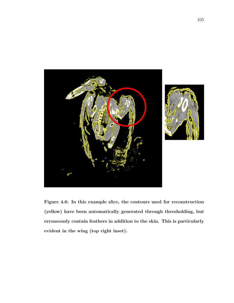
105

Figure 4.6: In this example slice, the contours used for reconstruction

(yellow) have been automatically generated through thresholding, but

erroneously contain feathers in addition to the skin. This is particularly

evident in the wing (top right inset).

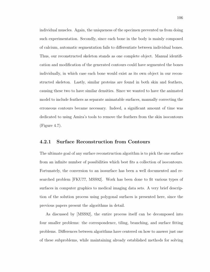
106

individual muscles. Again, the uniqueness of the specimen prevented us from doing

such experimentation. Secondly, since each bone in the body is mainly composed

of calcium, automatic segmentation fails to differentiate between individual bones.

Thus, our reconstructed skeleton stands as one complete object. Manual identifi-

cation and modification of the generated contours could have segmented the bones

individually, in which case each bone would exist as its own object in our recon-

structed skeleton. Lastly, similar proteins are found in both skin and feathers,

causing these two to have similar densities. Since we wanted to have the animated

model to include feathers as separate animatable surfaces, manually correcting the

erroneous contours became necessary. Indeed, a significant amount of time was

dedicated to using Amira’s tools to remove the feathers from the skin isocontours

(Figure 4.7).

4.2.1 Surface Reconstruction from Contours

The ultimate goal of any surface reconstruction algorithm is to pick the one surface

from an infinite number of possibilities which best fits a collection of isocontours.

Fortunately, the conversion to an isosurface has been a well documented and re-

searched problem [FKU77, MSS92]. Work has been done to fit various types of

surfaces in computer graphics to medical imaging data sets. A very brief descrip-

tion of the solution process using polygonal surfaces is presented here, since the

previous papers present the algorithms in detail.

As discussed by [MSS92], the entire process itself can be decomposed into

four smaller problems: the correspondence, tiling, branching, and surface fitting

problems. Differences between algorithms have centered on how to answer just one

of these subproblems, while maintaining already established methods for solving

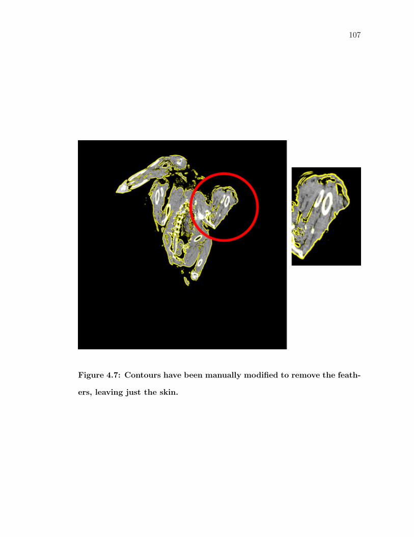
107

Figure 4.7: Contours have been manually modified to remove the feath-

ers, leaving just the skin.

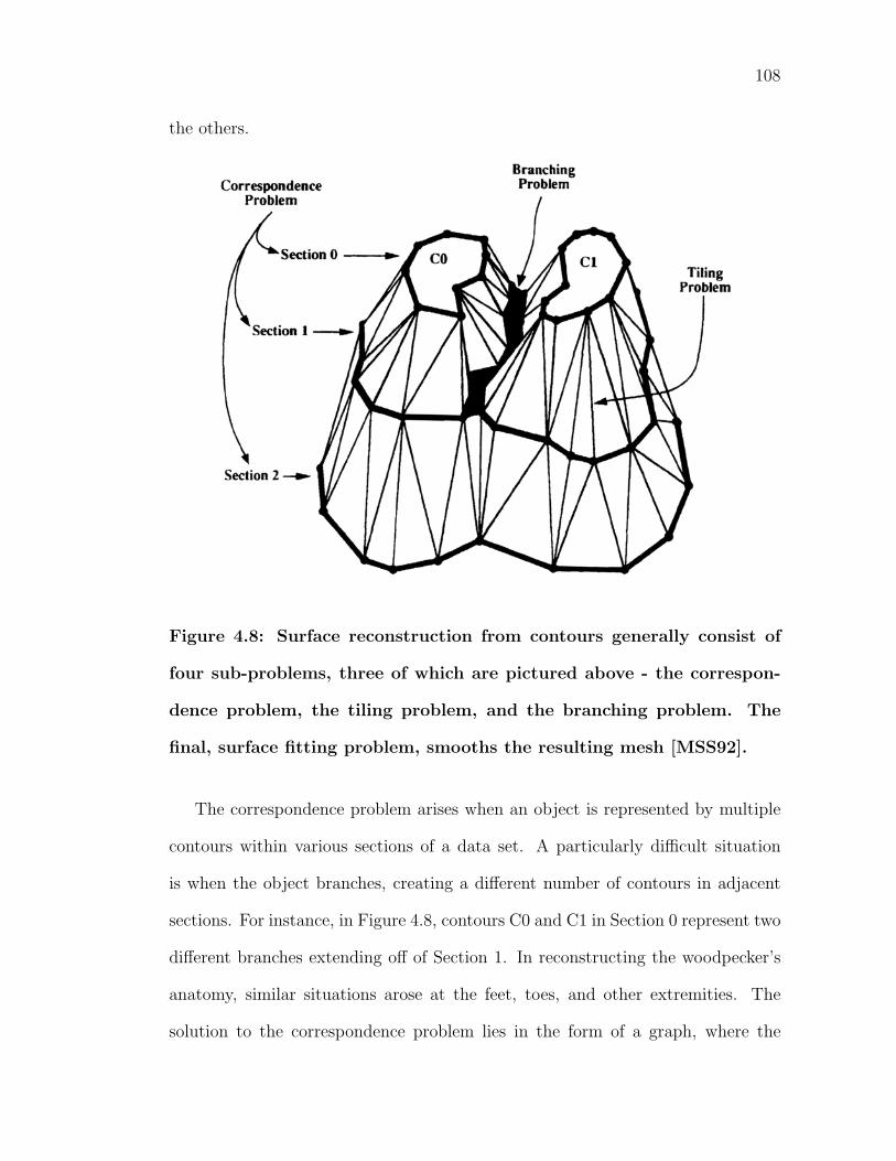
108

the others.

Figure 4.8: Surface reconstruction from contours generally consist of

four sub-problems, three of which are pictured above - the correspon-

dence problem, the tiling problem, and the branching problem. The

final, surface fitting problem, smooths the resulting mesh [MSS92].

The correspondence problem arises when an object is represented by multiple

contours within various sections of a data set. A particularly difficult situation

is when the object branches, creating a different number of contours in adjacent

sections. For instance, in Figure 4.8, contours C0 and C1 in Section 0 represent two

different branches extending off of Section 1. In reconstructing the woodpecker’s

anatomy, similar situations arose at the feet, toes, and other extremities. The

solution to the correspondence problem lies in the form of a graph, where the

109

nodes symbolize individual contours. Reflecting the general topological layout of

the dataset, the edges of the graph indicate which contours are linked. These edges

are laid using a function that analyzes contour size and shape and then connects

those most similar.

The tiling operation generates a polygonal surface by finding the most optimal

topological relationships. The correspondence problem determined which contours

are connected. Tiling now determines how they are connected. Objective functions

model constraints, such as minimizing surface area, but the problem is still typically

severely undetermined. User input is required. In our case, the Amira software

required specifying either the number of triangles in the final mesh to reduce

rendering speed later on or for the minimum edge length to maintain sufficient

resolution.

The tiling problem generally assumes that there is exactly a one to one ra-

tio of contours from each section. Since any branching violates this assumption,

the branching problem handles these exceptions. In this scenario, the pre-branch

section contains less contours than the post-branch. One approach divides the

pre-branch contour into two separate smaller contours, as in the case of Section 1

in Figure 4.8. Another common method forms composite contours from the post-

branch contours. The post-branching section is treated as if it were two sections.

Vertices and edges of minimum length connect multiple contours so that the newly

created section contains the same number of contours as the pre-branch section.

Meanwhile, the original information is used in the second section so that it matches

the contours of the next post-branch section.

Lastly, the resulting surface is smoothed during the optional final step, the

surface fitting problem. Algorithms of this nature are not exclusive to the recon-

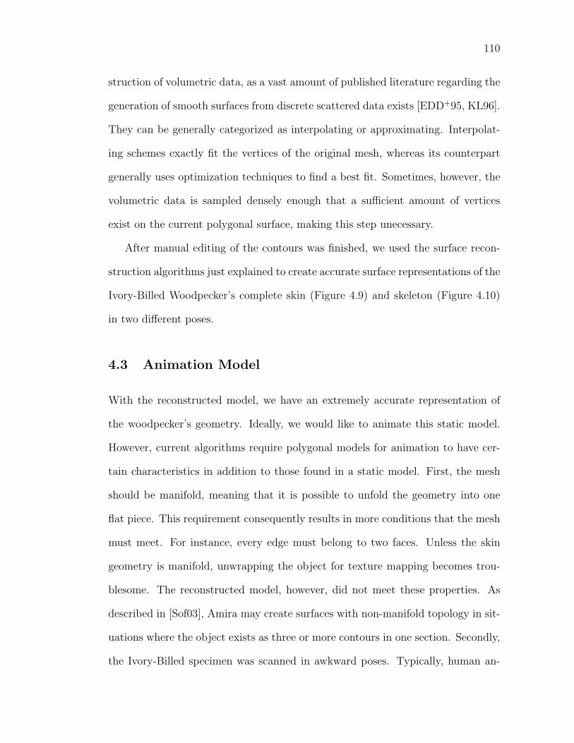
110

struction of volumetric data, as a vast amount of published literature regarding the

generation of smooth surfaces from discrete scattered data exists [EDD+95, KL96].

They can be generally categorized as interpolating or approximating. Interpolat-

ing schemes exactly fit the vertices of the original mesh, whereas its counterpart

generally uses optimization techniques to find a best fit. Sometimes, however, the

volumetric data is sampled densely enough that a sufficient amount of vertices

exist on the current polygonal surface, making this step unecessary.

After manual editing of the contours was finished, we used the surface recon-

struction algorithms just explained to create accurate surface representations of the

Ivory-Billed Woodpecker’s complete skin (Figure 4.9) and skeleton (Figure 4.10)

in two different poses.

4.3 Animation Model

With the reconstructed model, we have an extremely accurate representation of

the woodpecker’s geometry. Ideally, we would like to animate this static model.

However, current algorithms require polygonal models for animation to have cer-

tain characteristics in addition to those found in a static model. First, the mesh

should be manifold, meaning that it is possible to unfold the geometry into one

flat piece. This requirement consequently results in more conditions that the mesh

must meet. For instance, every edge must belong to two faces. Unless the skin

geometry is manifold, unwrapping the object for texture mapping becomes trou-

blesome. The reconstructed model, however, did not meet these properties. As

described in [Sof03], Amira may create surfaces with non-manifold topology in sit-

uations where the object exists as three or more contours in one section. Secondly,

the Ivory-Billed specimen was scanned in awkward poses. Typically, human an-

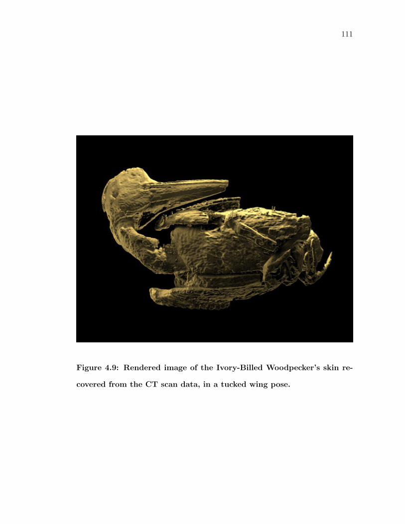
111

Figure 4.9: Rendered image of the Ivory-Billed Woodpecker’s skin re-

covered from the CT scan data, in a tucked wing pose.

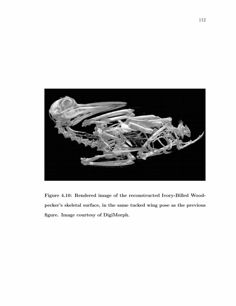
112

Figure 4.10: Rendered image of the reconstructed Ivory-Billed Wood-

pecker’s skeletal surface, in the same tucked wing pose as the previous

figure. Image courtesy of DigiMorph.

113

imated characters are modeled in a “crucifix-like” pose, with the arms extended

straight out from the shoulder, away from the torso. The legs usually extend

straight down, while the head points straight forward. Such positions make future

tasks in the animation pipeline easier. For instance, defining skeletal joints is easier

if the extremities lie in a straight line with the least amount of twisting. Lastly,

the reconstructed model had too many points - upwards of two million - for it to

be interactively manipulated in real-time with even the most powerful of graphics

cards.

Efficiency generally becomes a major concern when producing models for ani-

mation; character skin meshes should contain the least amount of points possible.

In our case, feathers will cover the majority of the skin mesh, so a large number of

points becomes unnecessary. Furthermore, thresholding during the reconstruction

phase generated contour edges that lie beneath the skin. These edges were carried

over into the reconstructed model, creating superfluous faces which are never seen

by the viewer. Thus, a less dense model, that is also optimized for animation, was

needed.

Several methods exist for representing geometry in computer graphics, but

only three are commonly used in animated models: polygons, parametric curved

surfaces (such as NURBS), and subdivision surfaces. Polygonal models, consisting

of mostly either triangles or rectangles, are the most basic of the three, but the

easiest to define objects of arbitrary complexity and topology. Unfortunately,

adding detailed information to parametric curved surfaces becomes difficult since

they specialize in producing an infinitely smooth surface [PT97]. A large number of

trimmed rectangular patches must be stitched together in order to form complex

shapes. Subdivision surfaces combine the strengths of polygonal modeling and

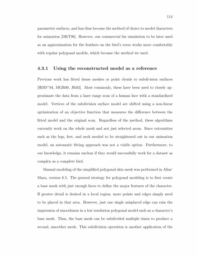
114

parametric surfaces, and has thus become the method of choice to model characters

for animation [DKT98]. However, our commercial fur simulation to be later used

as an approximation for the feathers on the bird’s torso works more comfortably

with regular polygonal models, which became the method we used.

4.3.1 Using the reconstructed model as a reference

Previous work has fitted dense meshes or point clouds to subdivision surfaces

[HDD+94, MGR00, JK02]. Most commonly, these have been used to closely ap-

proximate the data from a laser range scan of a human face with a standardized

model. Vertices of the subdivision surface model are shifted using a non-linear

optimization of an objective function that measures the difference between the

fitted model and the original scan. Regardless of the method, these algorithms

currently work on the whole mesh and not just selected areas. Since extremities

such as the legs, feet, and neck needed to be straightened out in our animation

model, an automatic fitting approach was not a viable option. Furthermore, to

our knowledge, it remains unclear if they would successfully work for a dataset as

complex as a complete bird.

Manual modeling of the simplified polygonal skin mesh was performed in Alias’

Maya, version 6.5. The general strategy for polygonal modeling is to first create

a base mesh with just enough faces to define the major features of the character.

If greater detail is desired in a local region, more points and edges simply need

to be placed in that area. However, just one single misplaced edge can ruin the

impression of smoothness in a low resolution polygonal model such as a character’s

base mesh. Thus, the base mesh can be subdivided multiple times to produce a

second, smoother mesh. This subdivision operation is another application of the

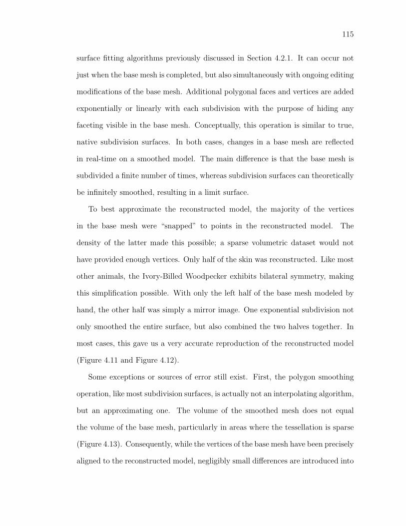
115

surface fitting algorithms previously discussed in Section 4.2.1. It can occur not

just when the base mesh is completed, but also simultaneously with ongoing editing

modifications of the base mesh. Additional polygonal faces and vertices are added

exponentially or linearly with each subdivision with the purpose of hiding any

faceting visible in the base mesh. Conceptually, this operation is similar to true,

native subdivision surfaces. In both cases, changes in a base mesh are reflected

in real-time on a smoothed model. The main difference is that the base mesh is

subdivided a finite number of times, whereas subdivision surfaces can theoretically

be infinitely smoothed, resulting in a limit surface.

To best approximate the reconstructed model, the majority of the vertices

in the base mesh were “snapped” to points in the reconstructed model. The

density of the latter made this possible; a sparse volumetric dataset would not

have provided enough vertices. Only half of the skin was reconstructed. Like most

other animals, the Ivory-Billed Woodpecker exhibits bilateral symmetry, making

this simplification possible. With only the left half of the base mesh modeled by

hand, the other half was simply a mirror image. One exponential subdivision not

only smoothed the entire surface, but also combined the two halves together. In

most cases, this gave us a very accurate reproduction of the reconstructed model

(Figure 4.11 and Figure 4.12).

Some exceptions or sources of error still exist. First, the polygon smoothing

operation, like most subdivision surfaces, is actually not an interpolating algorithm,

but an approximating one. The volume of the smoothed mesh does not equal

the volume of the base mesh, particularly in areas where the tessellation is sparse

(Figure 4.13). Consequently, while the vertices of the base mesh have been precisely

aligned to the reconstructed model, negligibly small differences are introduced into

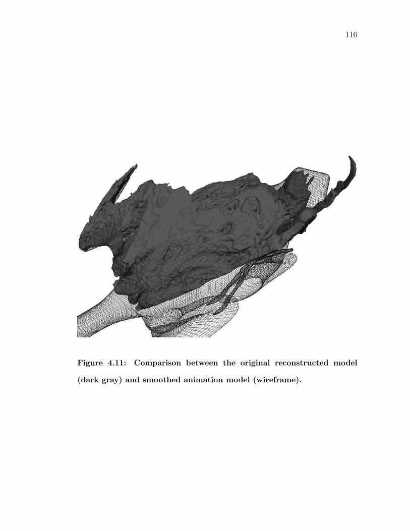
116

Figure 4.11: Comparison between the original reconstructed model

(dark gray) and smoothed animation model (wireframe).

117

Figure 4.12: Comparison between the original reconstructed model

(dark gray) and smoothed animation model (wireframe).

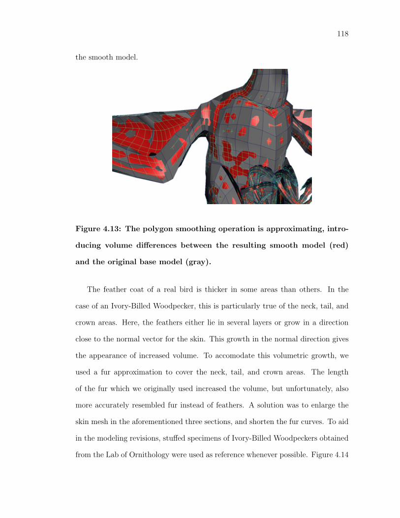
118

the smooth model.

Figure 4.13: The polygon smoothing operation is approximating, intro-

ducing volume differences between the resulting smooth model (red)

and the original base model (gray).

The feather coat of a real bird is thicker in some areas than others. In the

case of an Ivory-Billed Woodpecker, this is particularly true of the neck, tail, and

crown areas. Here, the feathers either lie in several layers or grow in a direction

close to the normal vector for the skin. This growth in the normal direction gives

the appearance of increased volume. To accomodate this volumetric growth, we

used a fur approximation to cover the neck, tail, and crown areas. The length

of the fur which we originally used increased the volume, but unfortunately, also

more accurately resembled fur instead of feathers. A solution was to enlarge the

skin mesh in the aforementioned three sections, and shorten the fur curves. To aid

in the modeling revisions, stuffed specimens of Ivory-Billed Woodpeckers obtained

from the Lab of Ornithology were used as reference whenever possible. Figure 4.14

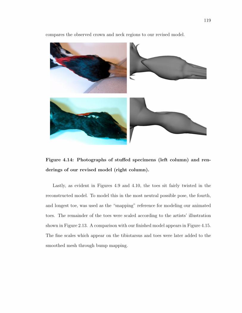
119

compares the observed crown and neck regions to our revised model.

Figure 4.14: Photographs of stuffed specimens (left column) and ren-

derings of our revised model (right column).

Lastly, as evident in Figures 4.9 and 4.10, the toes sit fairly twisted in the

reconstructed model. To model this in the most neutral possible pose, the fourth,

and longest toe, was used as the “snapping” reference for modeling our animated

toes. The remainder of the toes were scaled according to the artists’ illustration

shown in Figure 2.13. A comparison with our finished model appears in Figure 4.15.

The fine scales which appear on the tibiotarsus and toes were later added to the

smoothed mesh through bump mapping.

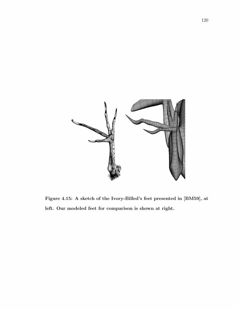
120

Figure 4.15: A sketch of the Ivory-Billed’s feet presented in [BM59], at

left. Our modeled feet for comparison is shown at right.

CHAPTER 5

ANIMATION OF SKIN MESH

5.1 Introduction to Animation Pipeline

Once modeling of the skin mesh is completed, the process to begin animating the

wingbeat begins. Setting up character controls, or the rig, is the first step. It

must be robust and flexible enough to cover the full range of motion desired for an

animation. The interface must also be intuitive and easy to control. In this thesis,

motion is parameterized mainly in the form of joints. During the actual animation

stage, these joints can be manipulated to make Ivory-Billed Woodpecker come to

life, regardless of whether or not the actual rediscovery is true.

Adding rigidity to otherwise soft tissue, a vertebrate’s skeletal system represents

a basis for which skeletal muscles can act on in order to induce motion. Bones and

joints exist in computer animation as well. Like their real-life counterparts, they

represent degrees of freedom upon which the body can articulate. In both cases,

a series bones can be connected together with other bones to create a hierarchy.

However, the similarities end there. Bones in computer animation lack explicit

geometrical information and are simply there to fill in the space between the joints.

The joints themselves serve as visual representations of transformation matrices

which define the rotation and offset from the parent joint. Often times, they may

not correspond to actual joints. For instance, facial animation can be driven using

shape interpolation or a set of joints that produces the desired deformation.

As part of the rigging process, a decision has to be made on how to manipu-

late these joints. While these joints can be used in a physical simulation of avian

flight, motion generated through standard animation techniques can fall under

121

122

three categories: inverse kinematics (IK), forward kinematics (FK), and procedu-

rally. Kinematics, itself, is defined as the study of an object’s motion without

considering the forces involved. Forward kinematics determines the position of a

linked, flexible object through specification of its joint angles. Inverse kinematics,

therefore, becomes the reverse. Given a target position in space or other con-

straints, IK solvers calculate the joint angles required for the object to reach that

position [ZB94]. Typically, the last joint in the chain, the end effector, carries

a handle specifying the desired location. This kind of functionality reduces the

amount of time required to produce an animation sequence since control over an

entire chain is reduced to just one parameter. Lastly, procedural animation typi-

cally employs mathematical equations to automatically adjust parameters without

user intervention.

Once our joints and rig is complete, these can be used to deform the skin mesh

through a process called smooth skinning [LCF00, KJP02]. Since each joint is

essentially a transformation matrix, a vertex can then become a weighted linear

sum of one or more of these transformation matrices. As the jonts are articulated,

they induce shape changes into the object, whose point p can be expressed as in

terms of the joint i by:

p =∑

wiTδi TL

i TWp p (5.1)

Since p is usually stored in the local space of the object in which it lies, TWp

transforms the point into world space. TLi converts a point from world space

into the coordinate frame defined by a stationary joint i. T δi are transformation

matrices that move the joint from its stationary pose to another position. wi is

the user-defined, normalized weight for joint i.

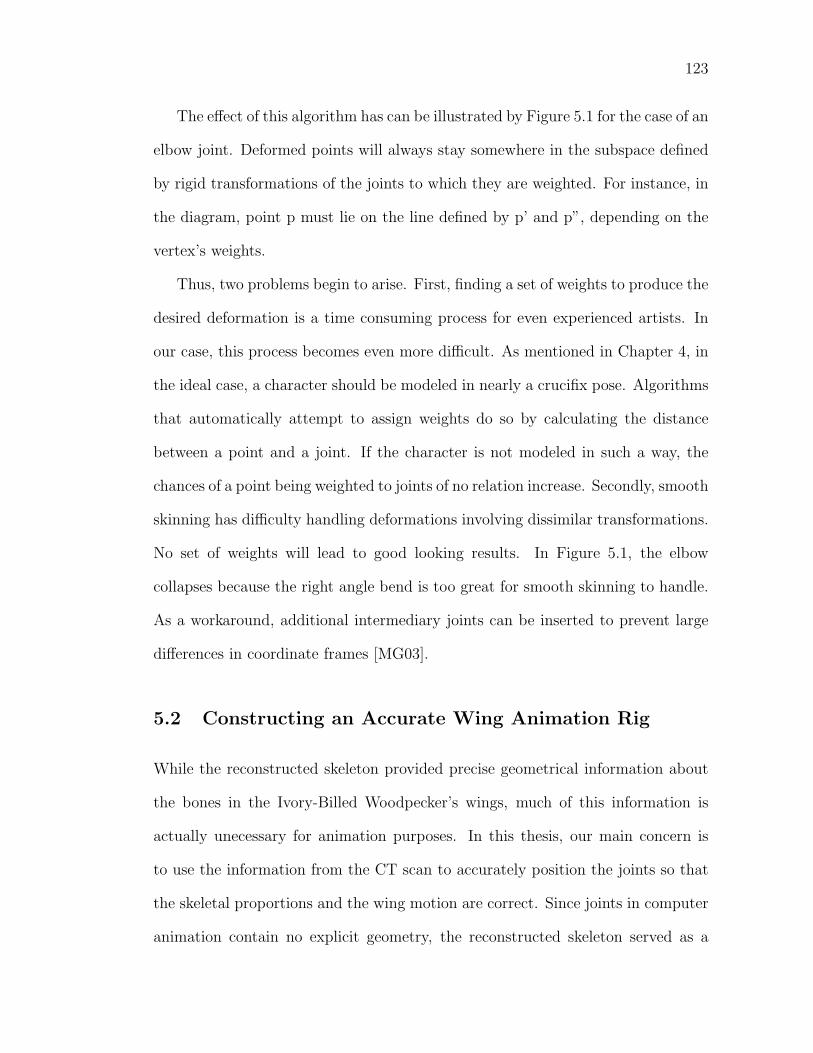
123

The effect of this algorithm has can be illustrated by Figure 5.1 for the case of an

elbow joint. Deformed points will always stay somewhere in the subspace defined

by rigid transformations of the joints to which they are weighted. For instance, in

the diagram, point p must lie on the line defined by p’ and p”, depending on the

vertex’s weights.

Thus, two problems begin to arise. First, finding a set of weights to produce the

desired deformation is a time consuming process for even experienced artists. In

our case, this process becomes even more difficult. As mentioned in Chapter 4, in

the ideal case, a character should be modeled in nearly a crucifix pose. Algorithms

that automatically attempt to assign weights do so by calculating the distance

between a point and a joint. If the character is not modeled in such a way, the

chances of a point being weighted to joints of no relation increase. Secondly, smooth

skinning has difficulty handling deformations involving dissimilar transformations.

No set of weights will lead to good looking results. In Figure 5.1, the elbow

collapses because the right angle bend is too great for smooth skinning to handle.

As a workaround, additional intermediary joints can be inserted to prevent large

differences in coordinate frames [MG03].

5.2 Constructing an Accurate Wing Animation Rig

While the reconstructed skeleton provided precise geometrical information about

the bones in the Ivory-Billed Woodpecker’s wings, much of this information is

actually unecessary for animation purposes. In this thesis, our main concern is

to use the information from the CT scan to accurately position the joints so that

the skeletal proportions and the wing motion are correct. Since joints in computer

animation contain no explicit geometry, the reconstructed skeleton served as a

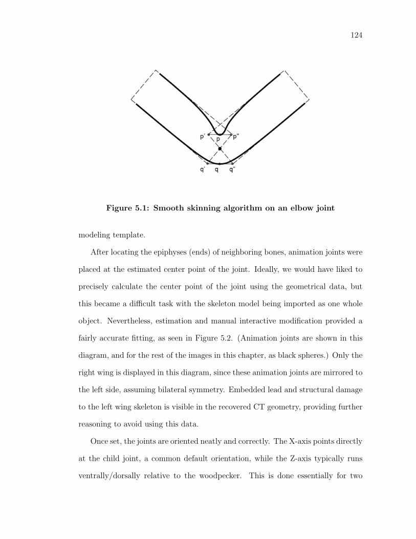
124

Figure 5.1: Smooth skinning algorithm on an elbow joint

modeling template.

After locating the epiphyses (ends) of neighboring bones, animation joints were

placed at the estimated center point of the joint. Ideally, we would have liked to

precisely calculate the center point of the joint using the geometrical data, but

this became a difficult task with the skeleton model being imported as one whole

object. Nevertheless, estimation and manual interactive modification provided a

fairly accurate fitting, as seen in Figure 5.2. (Animation joints are shown in this

diagram, and for the rest of the images in this chapter, as black spheres.) Only the

right wing is displayed in this diagram, since these animation joints are mirrored to

the left side, assuming bilateral symmetry. Embedded lead and structural damage

to the left wing skeleton is visible in the recovered CT geometry, providing further

reasoning to avoid using this data.

Once set, the joints are oriented neatly and correctly. The X-axis points directly

at the child joint, a common default orientation, while the Z-axis typically runs

ventrally/dorsally relative to the woodpecker. This is done essentially for two

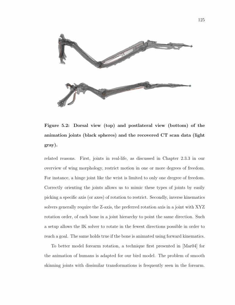
125

Figure 5.2: Dorsal view (top) and postlateral view (bottom) of the

animation joints (black spheres) and the recovered CT scan data (light

gray).

related reasons. First, joints in real-life, as discussed in Chapter 2.3.3 in our

overview of wing morphology, restrict motion in one or more degrees of freedom.

For instance, a hinge joint like the wrist is limited to only one dregree of freedom.

Correctly orienting the joints allows us to mimic these types of joints by easily

picking a specific axis (or axes) of rotation to restrict. Secondly, inverse kinematics

solvers generally require the Z-axis, the preferred rotation axis in a joint with XYZ

rotation order, of each bone in a joint hierarchy to point the same direction. Such

a setup allows the IK solver to rotate in the fewest directions possible in order to

reach a goal. The same holds true if the bone is animated using forward kinematics.

To better model forearm rotation, a technique first presented in [Mar04] for

the animation of humans is adapted for our bird model. The problem of smooth

skinning joints with dissimilar transformations is frequently seen in the forearm.

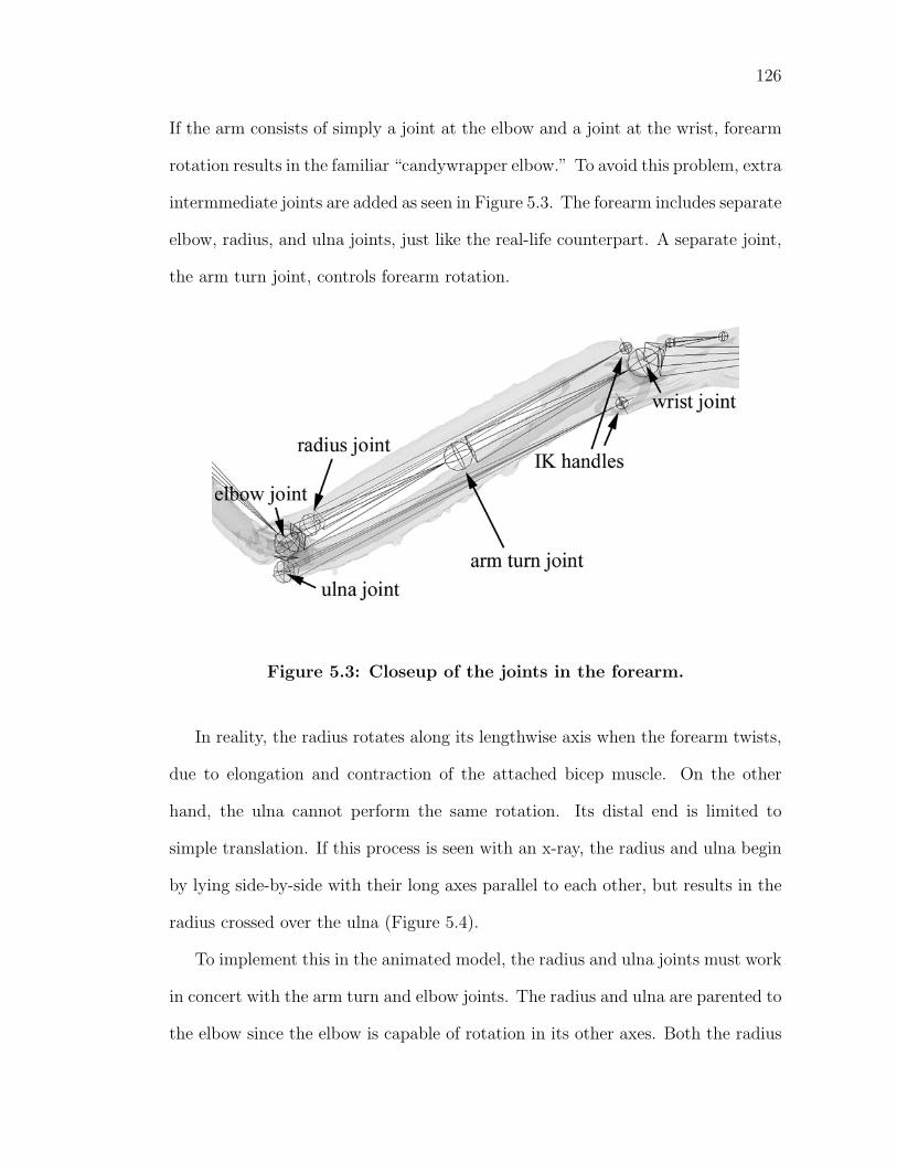
126

If the arm consists of simply a joint at the elbow and a joint at the wrist, forearm

rotation results in the familiar “candywrapper elbow.” To avoid this problem, extra

intermmediate joints are added as seen in Figure 5.3. The forearm includes separate

elbow, radius, and ulna joints, just like the real-life counterpart. A separate joint,

the arm turn joint, controls forearm rotation.

Figure 5.3: Closeup of the joints in the forearm.

In reality, the radius rotates along its lengthwise axis when the forearm twists,

due to elongation and contraction of the attached bicep muscle. On the other

hand, the ulna cannot perform the same rotation. Its distal end is limited to

simple translation. If this process is seen with an x-ray, the radius and ulna begin

by lying side-by-side with their long axes parallel to each other, but results in the

radius crossed over the ulna (Figure 5.4).

To implement this in the animated model, the radius and ulna joints must work

in concert with the arm turn and elbow joints. The radius and ulna are parented to

the elbow since the elbow is capable of rotation in its other axes. Both the radius

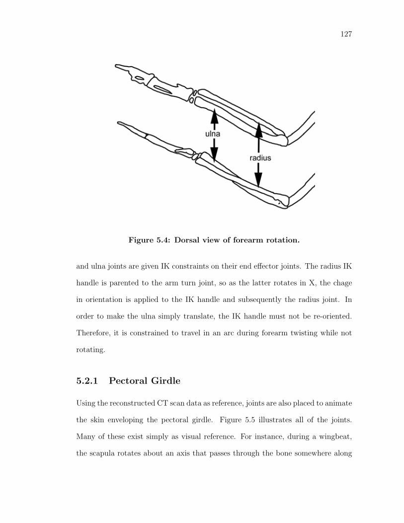
127

Figure 5.4: Dorsal view of forearm rotation.

and ulna joints are given IK constraints on their end effector joints. The radius IK

handle is parented to the arm turn joint, so as the latter rotates in X, the chage

in orientation is applied to the IK handle and subsequently the radius joint. In

order to make the ulna simply translate, the IK handle must not be re-oriented.

Therefore, it is constrained to travel in an arc during forearm twisting while not

rotating.

5.2.1 Pectoral Girdle

Using the reconstructed CT scan data as reference, joints are also placed to animate

the skin enveloping the pectoral girdle. Figure 5.5 illustrates all of the joints.

Many of these exist simply as visual reference. For instance, during a wingbeat,

the scapula rotates about an axis that passes through the bone somewhere along

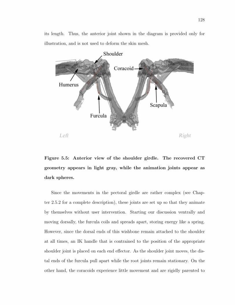
128

its length. Thus, the anterior joint shown in the diagram is provided only for

illustration, and is not used to deform the skin mesh.

Figure 5.5: Anterior view of the shoulder girdle. The recovered CT

geometry appears in light gray, while the animation joints appear as

dark spheres.

Since the movements in the pectoral girdle are rather complex (see Chap-

ter 2.5.2 for a complete description), these joints are set up so that they animate

by themselves without user intervention. Starting our discussion ventrally and

moving dorsally, the furcula coils and spreads apart, storing energy like a spring.

However, since the dorsal ends of this wishbone remain attached to the shoulder

at all times, an IK handle that is contrained to the position of the appropriate

shoulder joint is placed on each end effector. As the shoulder joint moves, the dis-

tal ends of the furcula pull apart while the root joints remain stationary. On the

other hand, the coracoids experience little movement and are rigidly parented to

129

the shoulder joint. Setup of the scapulas is similar to the furculas. An IK handle

is placed on the anterior end effector, and the offset between this and the shoulder

joint is constrained to remain constant. After smooth skinning is applied to mesh,

the furcular and scapular joints generate the most deformation while the coracoid

and shoulder joints stablize the region.

5.2.2 Patagium

The patagium is an example of where joints in animation do not find real-life coun-

terparts, but instead can be used to create a desired deformation. As introduced

in Chapter 2.3.3, the patagium is a flexible sheath of membrane that fills the space

between the shoulder, elbow, and wrist joints (see inset pictures in Figure 5.7).

Support comes from a tendon located on the leading edge, specifically the one

attached to the m. tensor propatagialis pars longa muscle. To animate this type

of elastic behavior, instead of using a continuous surface, the tendon is discretized

and its effects modeled by a stretchable joint chain (Figure 5.6). Note that this

kind of approach is not unlike those taken in true physical simulations which fre-

quently decompose continuous spaces into equivalent discrete spaces, such as in

finite element modeling, for the purposes of easier calcuation.

Additionally, even though animation joints will be responsible for replicating

this behavior, all of it should happen procedurally. The animator should have the

freedom to put the wing in any pose, and not have to worry about whether or not

the patagium will deform accordingly.

The first step is to create a skeletal chain that will automatically set itself in

the right orientation wherever the joints are placed. Observations show that the

patagium lie in approximately the same plane as the humerus, radius, and ulna

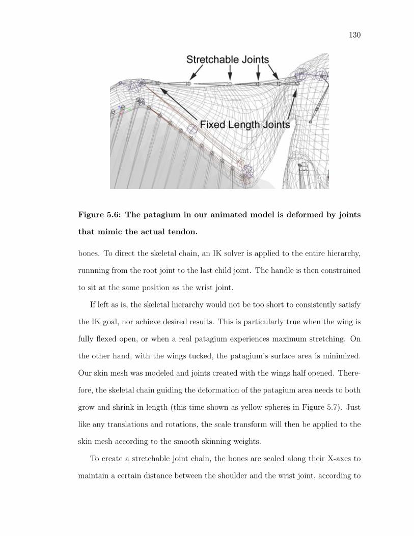
130

Figure 5.6: The patagium in our animated model is deformed by joints

that mimic the actual tendon.

bones. To direct the skeletal chain, an IK solver is applied to the entire hierarchy,

runnning from the root joint to the last child joint. The handle is then constrained

to sit at the same position as the wrist joint.

If left as is, the skeletal hierarchy would not be too short to consistently satisfy

the IK goal, nor achieve desired results. This is particularly true when the wing is

fully flexed open, or when a real patagium experiences maximum stretching. On

the other hand, with the wings tucked, the patagium’s surface area is minimized.

Our skin mesh was modeled and joints created with the wings half opened. There-

fore, the skeletal chain guiding the deformation of the patagium area needs to both

grow and shrink in length (this time shown as yellow spheres in Figure 5.7). Just

like any translations and rotations, the scale transform will then be applied to the

skin mesh according to the smooth skinning weights.

To create a stretchable joint chain, the bones are scaled along their X-axes to

maintain a certain distance between the shoulder and the wrist joint, according to

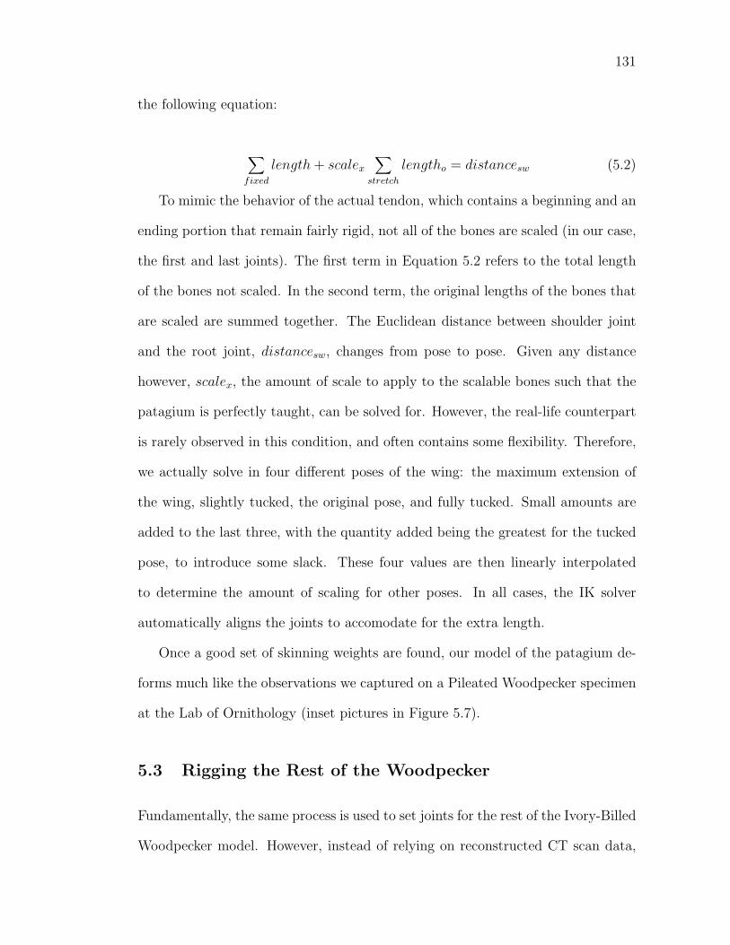
131

the following equation:

∑

fixed

length + scalex

∑

stretch

lengtho = distancesw (5.2)

To mimic the behavior of the actual tendon, which contains a beginning and an

ending portion that remain fairly rigid, not all of the bones are scaled (in our case,

the first and last joints). The first term in Equation 5.2 refers to the total length

of the bones not scaled. In the second term, the original lengths of the bones that

are scaled are summed together. The Euclidean distance between shoulder joint

and the root joint, distancesw, changes from pose to pose. Given any distance

however, scalex, the amount of scale to apply to the scalable bones such that the

patagium is perfectly taught, can be solved for. However, the real-life counterpart

is rarely observed in this condition, and often contains some flexibility. Therefore,

we actually solve in four different poses of the wing: the maximum extension of

the wing, slightly tucked, the original pose, and fully tucked. Small amounts are

added to the last three, with the quantity added being the greatest for the tucked

pose, to introduce some slack. These four values are then linearly interpolated

to determine the amount of scaling for other poses. In all cases, the IK solver

automatically aligns the joints to accomodate for the extra length.

Once a good set of skinning weights are found, our model of the patagium de-

forms much like the observations we captured on a Pileated Woodpecker specimen

at the Lab of Ornithology (inset pictures in Figure 5.7).

5.3 Rigging the Rest of the Woodpecker

Fundamentally, the same process is used to set joints for the rest of the Ivory-Billed

Woodpecker model. However, instead of relying on reconstructed CT scan data,

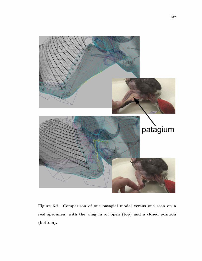
132

Figure 5.7: Comparison of our patagial model versus one seen on a

real specimen, with the wing in an open (top) and a closed position

(bottom).

133

joints are defined and characterized based on knowledge of the avian anatomy.

This is also another instance of where the joints in computer animation do not

necessarily concide with a real skeleton. In many cases, the amount of joints have

been reduced to make setting smooth skinning weights easier.

For instance, upwards of fourteen vertebrae are found in a real bird’s neck. In

our model, we employ only five (Figure 5.8), or just enough to replicate the same

degree of a freedom in the actual counterpart. Thus, although these simplifications

are made, the differences observed in the deformed skin mesh and in the real thing

are neglible.

Figure 5.8: Neck skeleton and rig.

However, providing the animator enough control over the skeleton so that one

can replicate the range of motion in the head/neck area presents a tough rigging

problem. To solve these, an IK handle is used to direct the position of the head.

As an example of how helpers are often made so that IK handles can be more

easily directed, the latter is parented to the blue box seen at the base of the head

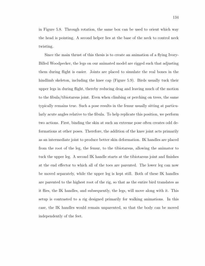
134

in Figure 5.8. Through rotation, the same box can be used to orient which way

the head is pointing. A second helper lies at the base of the neck to control neck

twisting.

Since the main thrust of this thesis is to create an animation of a flying Ivory-

Billed Woodpecker, the legs on our animated model are rigged such that adjusting

them during flight is easier. Joints are placed to simulate the real bones in the

hindlimb skeleton, including the knee cap (Figure 5.9). Birds usually tuck their

upper legs in during flight, thereby reducing drag and leaving much of the motion

to the fibula/tibiotarsus joint. Even when climbing or perching on trees, the same

typically remains true. Such a pose results in the femur usually sitting at particu-

larly acute angles relative to the fibula. To help replicate this position, we perform

two actions. First, binding the skin at such an extreme pose often creates odd de-

formations at other poses. Therefore, the addition of the knee joint acts primarily

as an intermediate joint to produce better skin deformation. IK handles are placed

from the root of the leg, the femur, to the tibiotarsus, allowing the animator to

tuck the upper leg. A second IK handle starts at the tibiotarsus joint and finishes

at the end effector to which all of the toes are parented. The lower leg can now

be moved separately, while the upper leg is kept still. Both of these IK handles

are parented to the highest root of the rig, so that as the entire bird translates as

it flies, the IK handles, and subsequently, the legs, will move along with it. This

setup is contrasted to a rig designed primarily for walking animations. In this

case, the IK handles would remain unparented, so that the body can be moved

independently of the feet.

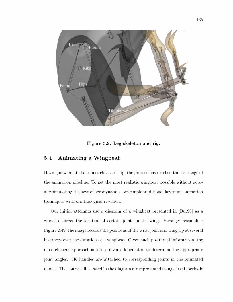
135

Figure 5.9: Leg skeleton and rig.

5.4 Animating a Wingbeat

Having now created a robust character rig, the process has reached the last stage of

the animation pipeline. To get the most realistic wingbeat possible without actu-

ally simulating the laws of aerodynamics, we couple traditional keyframe animation

techinques with ornithological research.

Our initial attempts use a diagram of a wingbeat presented in [Bur90] as a

guide to direct the location of certain joints in the wing. Strongly resembling

Figure 2.49, the image records the positions of the wrist joint and wing tip at several

instances over the duration of a wingbeat. Given such positional information, the

most efficient approach is to use inverse kinematics to determine the appropriate

joint angles. IK handles are attached to corresponding joints in the animated

model. The courses illustrated in the diagram are represented using closed, periodic

136

parametric curves, to which the handles can be attached to follow as motion paths.

Key frames can then be set, relating the parametric values of the curve versus time.

However, through experimentation, using IK to position the wings traded away

too much control over each individual joint. The animation of a wingbeat is com-

plex enough that an animator needs finer management. For instance, when an IK

handle is animated, usually all of the joints will rotate, making it impossible to

apply rotation to just a single joint in the wing. Furthermore, with only a few

joints in the wing, any time saved by using IK is neglible compared to sacrifice

made over directability. Lastly, the majority of struggle is due to the most widely

cited disadvantage concerning inverse kinematics: as a mathematical problem, IK

is inherently underdetermined. Several, if not inifinite, poses are possible to satisfy

a target goal, even after refining the solution with more constraints.

Left with forward kinematics, equivalent data is needed to animate a wingbeat.

Fortunately, [DGJ91] and [JJDGJ88] presented kinematic studies of avian flight

where they used high speed x-rays to record a wingbeat. In actuality, their studies

serve largely as a unique form of motion capture.

The former, in particular, documented the rotation angle of each joint in the

wing as a function of time (see Figure 2.42). However, for the humerus ball joint,

they plot measurements in terms of a world space coordinate frame and not in a

local space coordinate frame for the joint. Thus, a change of basis matrix needs to

be applied before the values are keyframed.

Much of what is described by [JJDGJ88] has already been implemented into

the pectoral girdle during the rigging stage. In order to trigger the procedural

animation we created, the shoulder joints need to be translated because the other

joints or IK solvers were constrained to these two joints. Translation is set to

137

occur automatically in terms of the elevation and depression of the humerus. As

the humerus is raised, the shoulder joints spread apart and as the humerus is

lowered, the shoulder joint come closer together.

CHAPTER 6

FEATHERING

A continuous, textured polygonal surface may suffice as a satisfactory repre-

sentation for many situations. However, truly photorealistic renderings of a bird

require displaying individual feather objects.

As implied in the Chapter 3, simulating convincing feathers is a four-part chal-

lenge. First, a model must capture the hierarchical structure of an individual

feather, complete with its overall silhouette shape, rachis, barbs, and possibly

barbules. Structural variation between different types complicates any algorithm.

Secondly, with thousands of feathers on a bird, it becomes important to distribute

them not just quickly, but also such that they accurately represent the bird’s aero-

dynamic profile. Once positioned and aligned in a still pose, animating these feath-

ers presents the next problem. Geometrical changes occur on two levels: within

a single feather as it responds to aerodynamic loading as well as the geometric

arrangement of feathers as a whole. Interpenetration must be prevented while

simulating these continually changing geometries. Lastly, modeling the complex

light reflections of a feather remains the final issue.

This chapter mainly focuses on modeling, distributing, and animating the flight

feathers of the Ivory-Billed Woodpecker. The other feathers will be approximated

using commercially available software usually used for fur.

6.1 Modeling Individual Flight Feathers

Due to the large number of feathers on a bird, modeling feathers quickly be-

comes a memory-consuming task. In the previous works chapter, we outlined past

techniques which have been implemented to model a single feather. All of these

138

139

paradigms use curves or thin strips of polygons to represent a single barb. Such

methods require storing at least several points or control vertices for each barb,

and possibly thousands for a feather. Since future applications of our work may

include interactive displays which can animate a bird in real-time, our solution

must be computationally efficient.

Using parametric surfaces vastly reduces the number of control vertices per

feather. Surfaces dependent on two parametric variables (U and V) form con-

tinuous, infinitely smooth geometry. Modeling the exact shape can be achieved

by adjusting the control vertices’ positions, which are likewise stored in a two di-

mensional array. Although many types of parametric surfaces exist, in this thesis,

we use the Maya-supported nonuniform rational B-spline surfaces (or NURBS)

[PT97].

Our general strategy for procedurally constructing a flight feather is to model

each feather vane as a nearly flat, trimmed NURBS surface. The vane planes,

created through a lofting operation, are trimmed to the desired shape using user-

specified curves. Barbs are created using distortion mapping techniques on the

surface of the vanes. Along with the rachis, which also is a NURBS surface by

itself, the vanes are smooth-skinned to a set of animation bones. Instead of having

to adjust every control vertex individually, the joints provide simple controls to

deform the previously flat vanes, such as the lengthwise curvature that occurs

naturally in feathers. A Maya Embedded Language script performs these tasks,

further speeding up the process of modeling the forty-two flight feathers located

on the Ivory-Billed Woodpecker’s wings.

Thus, the first step of our flight feather construction pipeline begins with defin-

ing a pair of connected bones for each feather while the bird’s wing is spread open

140

and lying nearly in the frontal plane. The root joint provides orientation informa-

tion for each feather throughout its construction. Furthermore, it is oriented so

that its local orthonormal basis lies at a known relationship relative to the bird:

the X-direction, as in the case with almost all animation joints, faces directly at

the child joint, the Y-direction points laterally, towards the bird’s midline, and

the Z-direction faces ventrally (Figure 6.1). Since our feathers are first modeled as

nearly flat planes, a finished model lies therefore primarily within the XY-plane.

Even though Maya generally stores locations in world space, all operations relat-

ing to feather construction can be assumed to occur in this ‘bone space,” unless

otherwise specified. Next on the joint hierarchy, rotation of the root joint’s child

introduces either lengthwise curvature or twist, depending on the direction of ro-

tation. We will refer to this joint as the “twist joint.” The third and final joint,

in conjunction with the first joint, defines the length of the feather. Once these

bones are created and distributed for each flight feather, the rest of the operations

occur within the scripted interface.

6.1.1 Rachis modeling

In modeling the geometry of the rachis, our primary concern is to capture three

important observations: the cross-sectional profile of a rachis, its lengthwise taper,

and its relative curvature. To best do this, we extrude a cross sectional profile

along a user defined curve. Subsequent scaling of the resulting NURBS surface

creates the tapering.

A parametric curve guides the extrusion of the rachis profile. The first and

last control vertices are located at the root and final joints of the feather bone

hierarchy, respectively. Within the feather construction interface, the user can

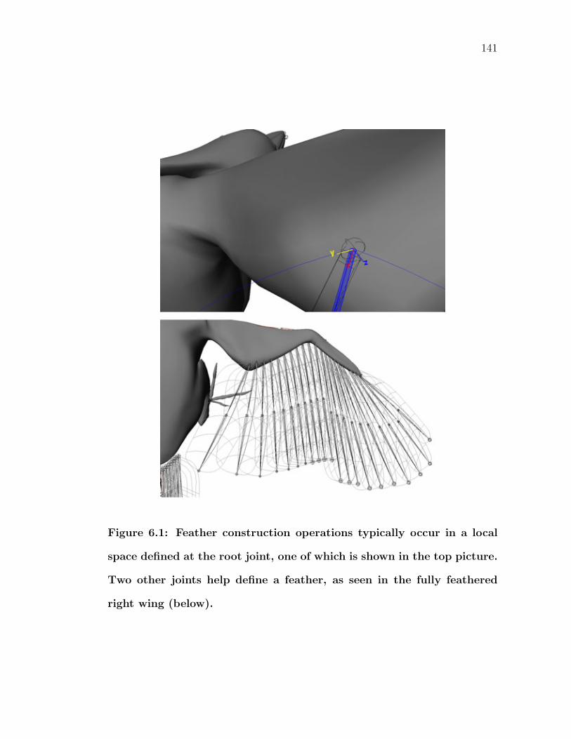
141

Figure 6.1: Feather construction operations typically occur in a local

space defined at the root joint, one of which is shown in the top picture.

Two other joints help define a feather, as seen in the fully feathered

right wing (below).

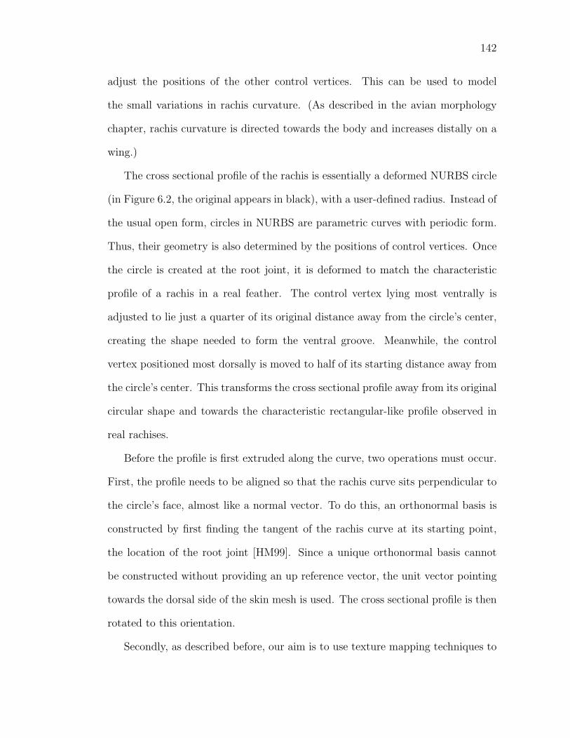
142

adjust the positions of the other control vertices. This can be used to model

the small variations in rachis curvature. (As described in the avian morphology

chapter, rachis curvature is directed towards the body and increases distally on a

wing.)

The cross sectional profile of the rachis is essentially a deformed NURBS circle

(in Figure 6.2, the original appears in black), with a user-defined radius. Instead of

the usual open form, circles in NURBS are parametric curves with periodic form.

Thus, their geometry is also determined by the positions of control vertices. Once

the circle is created at the root joint, it is deformed to match the characteristic

profile of a rachis in a real feather. The control vertex lying most ventrally is

adjusted to lie just a quarter of its original distance away from the circle’s center,

creating the shape needed to form the ventral groove. Meanwhile, the control

vertex positioned most dorsally is moved to half of its starting distance away from

the circle’s center. This transforms the cross sectional profile away from its original

circular shape and towards the characteristic rectangular-like profile observed in

real rachises.

Before the profile is first extruded along the curve, two operations must occur.

First, the profile needs to be aligned so that the rachis curve sits perpendicular to

the circle’s face, almost like a normal vector. To do this, an orthonormal basis is

constructed by first finding the tangent of the rachis curve at its starting point,

the location of the root joint [HM99]. Since a unique orthonormal basis cannot

be constructed without providing an up reference vector, the unit vector pointing

towards the dorsal side of the skin mesh is used. The cross sectional profile is then

rotated to this orientation.

Secondly, as described before, our aim is to use texture mapping techniques to

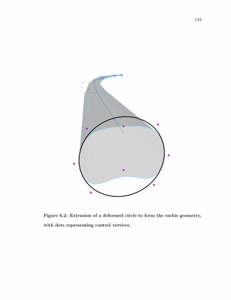
143

Figure 6.2: Extrusion of a deformed circle to form the rachis geometry,

with dots representing control vertices.

144

create the illusion of barbs. Although a key feature of NURBS surfaces is that

their parameterization can be non-uniform, we strive to keep all of the feather

surfaces fairly close to uniform parameterization. With NURBS surfaces, Maya

directly uses the UV parameterization as texture coordinates. Therefore, any dis-

tortion away from uniformity will also distort a texture-mapped image. While the

rachis path curve was originally constructed with uniform parameterization, user

interaction to shape the curvature in the rachis likely changed this characteristic.

This needs to be modified before extrusion, or else the extruded surface will carry

the same non-uniformity.

The profile is first extruded along the rachis curve to form a NURBS tube of

uniform thickness. This operation sweeps the cross-sectional profile along a path

to form a three-dimensional surface (light gray) (Figure 6.2). As the cross section

travels along the path, it rotates to keep a fixed reference vector, the profile’s

y-axis, tangent to the path. This kind of extrusion is called a “directed-at,” as

opposed to a “flat” extrusion which ignores the orientation of the profile in relation

to the curve. With the extrusion complete, we have a surface that not only has

the same parameterization in the U direction as the original cross-section, but also

has the same number of control vertices in the V direction as the path.

To introduce the taper seen in rachises, we uniformly scale the cross-section

so that it decreases exponentially farther down the rachis curve, according to the

following formula:

scale = e−distance/lengthrachis (6.1)

where distance is the distance between the control vertices and lengthrachis is

the total length of the rachis curve.

145

6.1.2 Vane modeling

To begin creation of the NURBS surfaces which will represent the feather vanes, the

rachis curve is duplicated and translated laterally in the y-direction. The amount

and direction of translation depends on whether it is an inner vane or outer plane.

Once the translation is complete, a loft operation between the two curves creates

a NURBS surface with the same degree parameterization in the U direction as the

curves (Figure 6.3). In the V direction, the surface is cubic and constant U values

form isoparametric straight lines.

Figure 6.3: Vane modeling starts with a loft operation to form a flat

NURBS surface.

However, this kind of rectangular layout of the isoparametric curves1 makes

texturing more difficult, particularly in the application of distortion maps to rep-

resent the barbs of a feather vane. Recall that NURBS surfaces use their intrinsic

parameterization as texture coordinates. If left as is, we would need to create a

texture map of curved lines to simulate the barbs’ acute angle with respect to the

rachis and length-wise curvature. These lines need to be closely packed together as

1An isoparametric curve (“isoparm”) is a curve in parametric space with onevariable kept constant.

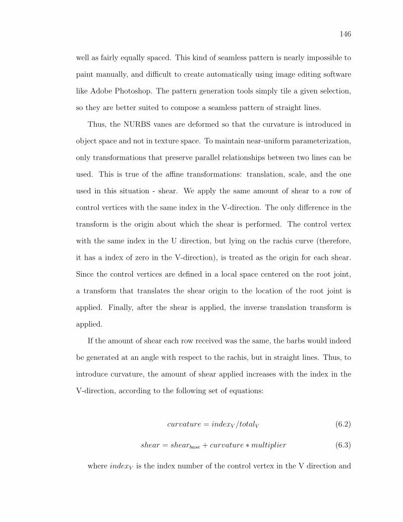
146

well as fairly equally spaced. This kind of seamless pattern is nearly impossible to

paint manually, and difficult to create automatically using image editing software

like Adobe Photoshop. The pattern generation tools simply tile a given selection,

so they are better suited to compose a seamless pattern of straight lines.

Thus, the NURBS vanes are deformed so that the curvature is introduced in

object space and not in texture space. To maintain near-uniform parameterization,

only transformations that preserve parallel relationships between two lines can be

used. This is true of the affine transformations: translation, scale, and the one

used in this situation - shear. We apply the same amount of shear to a row of

control vertices with the same index in the V-direction. The only difference in the

transform is the origin about which the shear is performed. The control vertex

with the same index in the U direction, but lying on the rachis curve (therefore,

it has a index of zero in the V-direction), is treated as the origin for each shear.

Since the control vertices are defined in a local space centered on the root joint,

a transform that translates the shear origin to the location of the root joint is

applied. Finally, after the shear is applied, the inverse translation transform is

applied.

If the amount of shear each row received was the same, the barbs would indeed

be generated at an angle with respect to the rachis, but in straight lines. Thus, to

introduce curvature, the amount of shear applied increases with the index in the

V-direction, according to the following set of equations:

curvature = indexV /totalV (6.2)

shear = shearbase + curvature ∗ multiplier (6.3)

where indexV is the index number of the control vertex in the V direction and

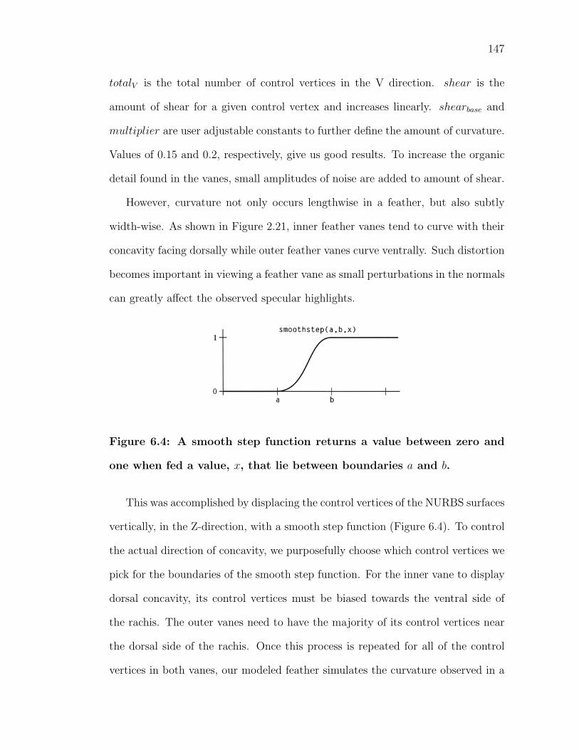
147

totalV is the total number of control vertices in the V direction. shear is the

amount of shear for a given control vertex and increases linearly. shearbase and

multiplier are user adjustable constants to further define the amount of curvature.

Values of 0.15 and 0.2, respectively, give us good results. To increase the organic

detail found in the vanes, small amplitudes of noise are added to amount of shear.

However, curvature not only occurs lengthwise in a feather, but also subtly

width-wise. As shown in Figure 2.21, inner feather vanes tend to curve with their

concavity facing dorsally while outer feather vanes curve ventrally. Such distortion

becomes important in viewing a feather vane as small perturbations in the normals

can greatly affect the observed specular highlights.

Figure 6.4: A smooth step function returns a value between zero and

one when fed a value, x, that lie between boundaries a and b.

This was accomplished by displacing the control vertices of the NURBS surfaces

vertically, in the Z-direction, with a smooth step function (Figure 6.4). To control

the actual direction of concavity, we purposefully choose which control vertices we

pick for the boundaries of the smooth step function. For the inner vane to display

dorsal concavity, its control vertices must be biased towards the ventral side of

the rachis. The outer vanes need to have the majority of its control vertices near

the dorsal side of the rachis. Once this process is repeated for all of the control

vertices in both vanes, our modeled feather simulates the curvature observed in a

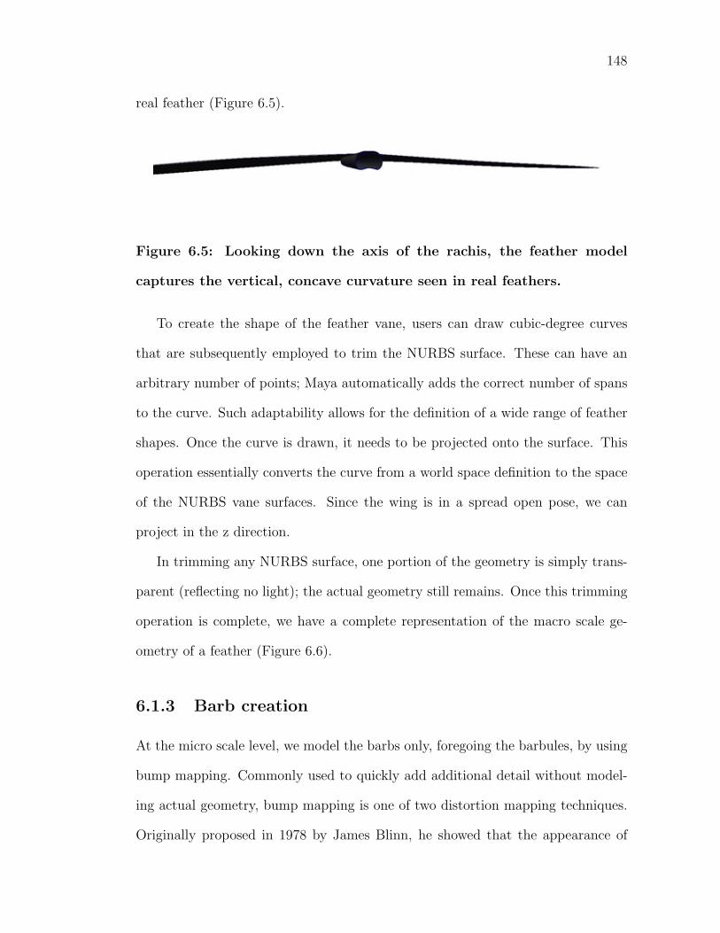
148

real feather (Figure 6.5).

Figure 6.5: Looking down the axis of the rachis, the feather model

captures the vertical, concave curvature seen in real feathers.

To create the shape of the feather vane, users can draw cubic-degree curves

that are subsequently employed to trim the NURBS surface. These can have an

arbitrary number of points; Maya automatically adds the correct number of spans

to the curve. Such adaptability allows for the definition of a wide range of feather

shapes. Once the curve is drawn, it needs to be projected onto the surface. This

operation essentially converts the curve from a world space definition to the space

of the NURBS vane surfaces. Since the wing is in a spread open pose, we can

project in the z direction.

In trimming any NURBS surface, one portion of the geometry is simply trans-

parent (reflecting no light); the actual geometry still remains. Once this trimming

operation is complete, we have a complete representation of the macro scale ge-

ometry of a feather (Figure 6.6).

6.1.3 Barb creation

At the micro scale level, we model the barbs only, foregoing the barbules, by using

bump mapping. Commonly used to quickly add additional detail without model-

ing actual geometry, bump mapping is one of two distortion mapping techniques.

Originally proposed in 1978 by James Blinn, he showed that the appearance of

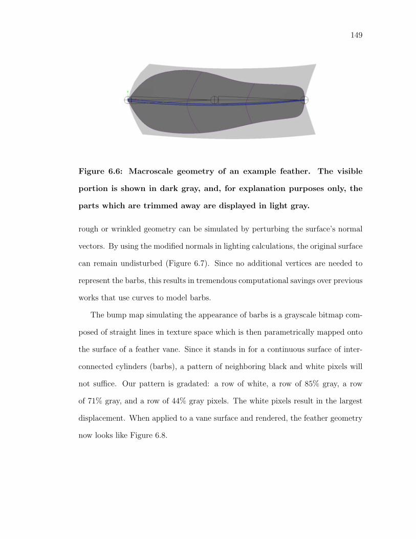
149

Figure 6.6: Macroscale geometry of an example feather. The visible

portion is shown in dark gray, and, for explanation purposes only, the

parts which are trimmed away are displayed in light gray.

rough or wrinkled geometry can be simulated by perturbing the surface’s normal

vectors. By using the modified normals in lighting calculations, the original surface

can remain undisturbed (Figure 6.7). Since no additional vertices are needed to

represent the barbs, this results in tremendous computational savings over previous

works that use curves to model barbs.

The bump map simulating the appearance of barbs is a grayscale bitmap com-

posed of straight lines in texture space which is then parametrically mapped onto

the surface of a feather vane. Since it stands in for a continuous surface of inter-

connected cylinders (barbs), a pattern of neighboring black and white pixels will

not suffice. Our pattern is gradated: a row of white, a row of 85% gray, a row

of 71% gray, and a row of 44% gray pixels. The white pixels result in the largest

displacement. When applied to a vane surface and rendered, the feather geometry

now looks like Figure 6.8.

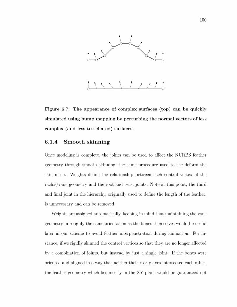
150

Figure 6.7: The appearance of complex surfaces (top) can be quickly

simulated using bump mapping by perturbing the normal vectors of less

complex (and less tessellated) surfaces.

6.1.4 Smooth skinning

Once modeling is complete, the joints can be used to affect the NURBS feather

geometry through smooth skinning, the same procedure used to the deform the

skin mesh. Weights define the relationship between each control vertex of the

rachis/vane geometry and the root and twist joints. Note at this point, the third

and final joint in the hierarchy, originally used to define the length of the feather,

is unnecessary and can be removed.

Weights are assigned automatically, keeping in mind that maintaining the vane

geometry in roughly the same orientation as the bones themselves would be useful

later in our scheme to avoid feather interpenetration during animation. For in-

stance, if we rigidly skinned the control vertices so that they are no longer affected

by a combination of joints, but instead by just a single joint. If the bones were

oriented and aligned in a way that neither their x or y axes intersected each other,

the feather geometry which lies mostly in the XY plane would be guaranteed not

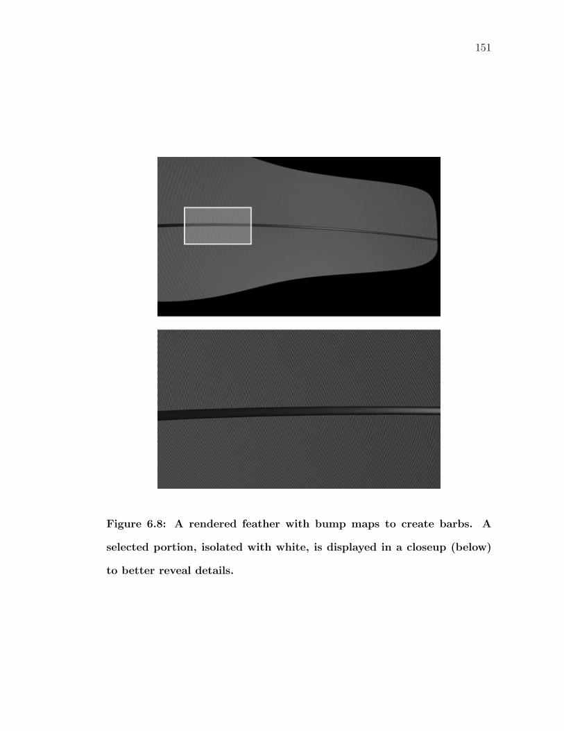
151

Figure 6.8: A rendered feather with bump maps to create barbs. A

selected portion, isolated with white, is displayed in a closeup (below)

to better reveal details.

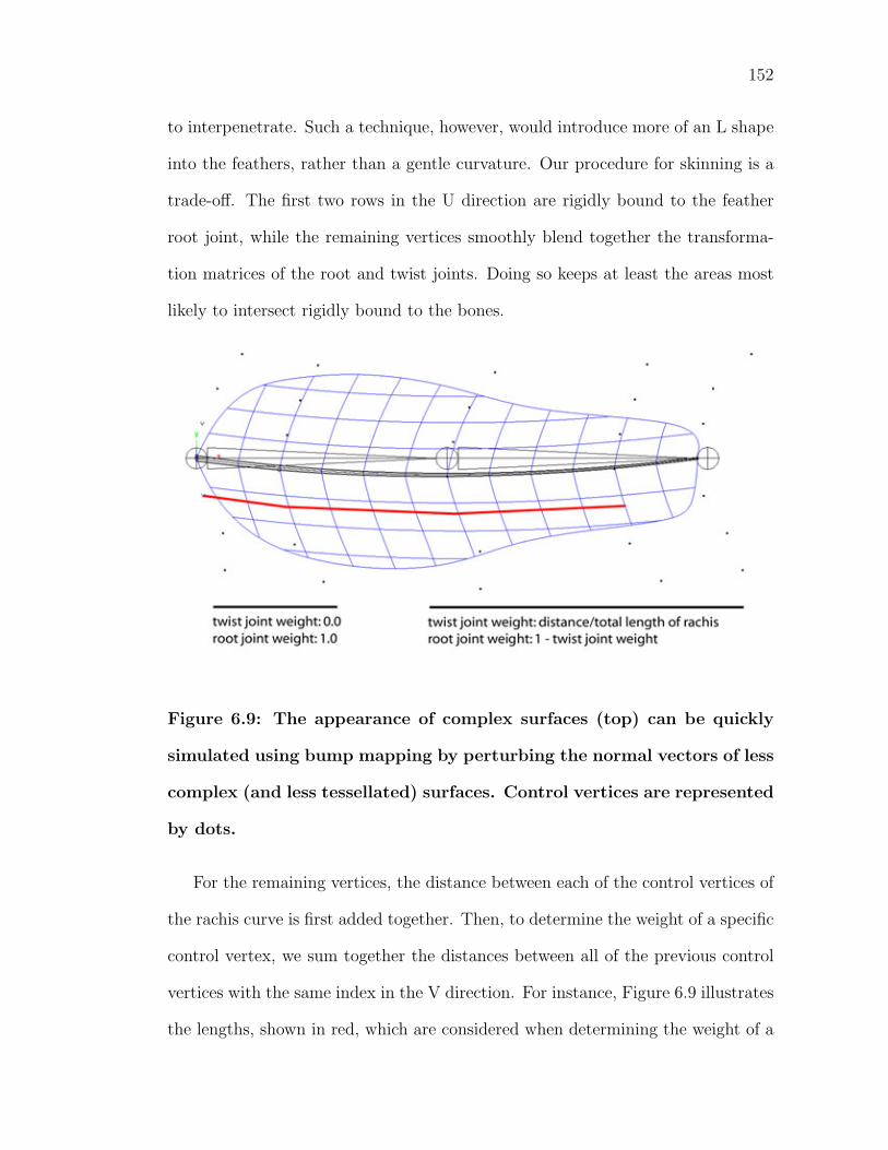
152

to interpenetrate. Such a technique, however, would introduce more of an L shape

into the feathers, rather than a gentle curvature. Our procedure for skinning is a

trade-off. The first two rows in the U direction are rigidly bound to the feather

root joint, while the remaining vertices smoothly blend together the transforma-

tion matrices of the root and twist joints. Doing so keeps at least the areas most

likely to intersect rigidly bound to the bones.

Figure 6.9: The appearance of complex surfaces (top) can be quickly

simulated using bump mapping by perturbing the normal vectors of less

complex (and less tessellated) surfaces. Control vertices are represented

by dots.

For the remaining vertices, the distance between each of the control vertices of

the rachis curve is first added together. Then, to determine the weight of a specific

control vertex, we sum together the distances between all of the previous control

vertices with the same index in the V direction. For instance, Figure 6.9 illustrates

the lengths, shown in red, which are considered when determining the weight of a

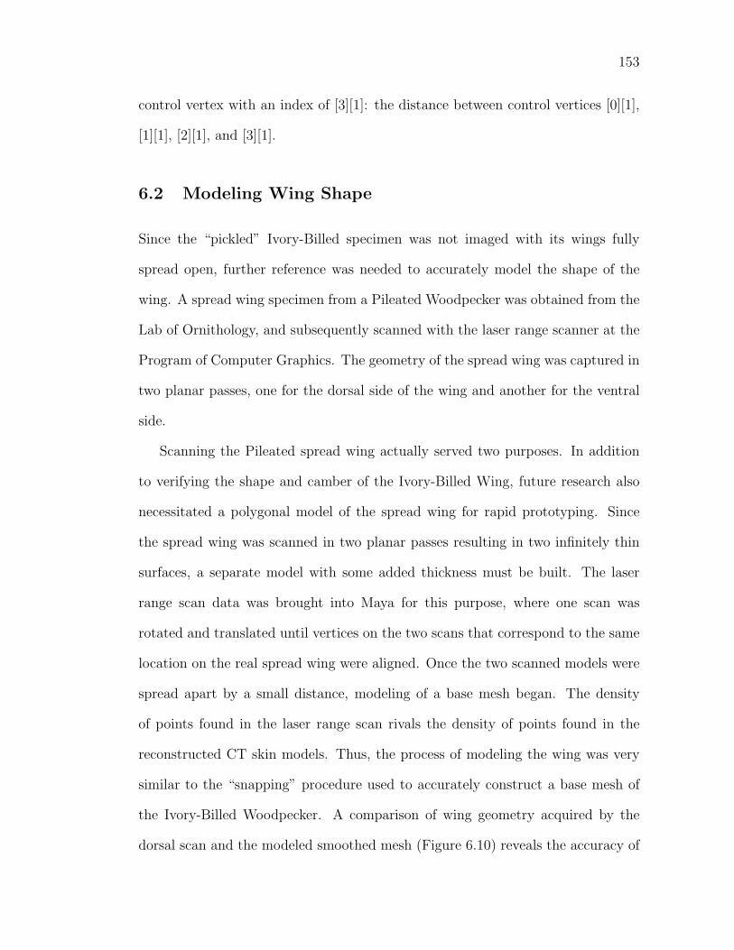
153

control vertex with an index of [3][1]: the distance between control vertices [0][1],

[1][1], [2][1], and [3][1].

6.2 Modeling Wing Shape

Since the “pickled” Ivory-Billed specimen was not imaged with its wings fully

spread open, further reference was needed to accurately model the shape of the

wing. A spread wing specimen from a Pileated Woodpecker was obtained from the

Lab of Ornithology, and subsequently scanned with the laser range scanner at the

Program of Computer Graphics. The geometry of the spread wing was captured in

two planar passes, one for the dorsal side of the wing and another for the ventral

side.

Scanning the Pileated spread wing actually served two purposes. In addition

to verifying the shape and camber of the Ivory-Billed Wing, future research also

necessitated a polygonal model of the spread wing for rapid prototyping. Since

the spread wing was scanned in two planar passes resulting in two infinitely thin

surfaces, a separate model with some added thickness must be built. The laser

range scan data was brought into Maya for this purpose, where one scan was

rotated and translated until vertices on the two scans that correspond to the same

location on the real spread wing were aligned. Once the two scanned models were

spread apart by a small distance, modeling of a base mesh began. The density

of points found in the laser range scan rivals the density of points found in the

reconstructed CT skin models. Thus, the process of modeling the wing was very

similar to the “snapping” procedure used to accurately construct a base mesh of

the Ivory-Billed Woodpecker. A comparison of wing geometry acquired by the

dorsal scan and the modeled smoothed mesh (Figure 6.10) reveals the accuracy of

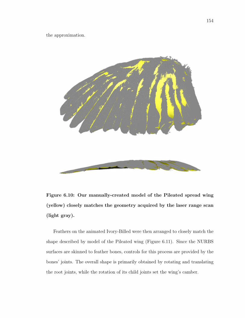
154

the approximation.

Figure 6.10: Our manually-created model of the Pileated spread wing

(yellow) closely matches the geometry acquired by the laser range scan

(light gray).

Feathers on the animated Ivory-Billed were then arranged to closely match the

shape described by model of the Pileated wing (Figure 6.11). Since the NURBS

surfaces are skinned to feather bones, controls for this process are provided by the

bones’ joints. The overall shape is primarily obtained by rotating and translating

the root joints, while the rotation of its child joints set the wing’s camber.

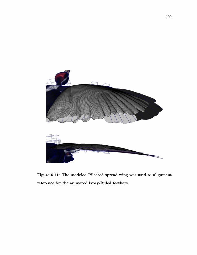
155

Figure 6.11: The modeled Pileated spread wing was used as alignment

reference for the animated Ivory-Billed feathers.

156

6.3 Flight Feather Animation

6.3.1 Wings

As one of the major challenges in this thesis, the flight feathers on the wing should

automatically align themselves according to how the bones in the wing are posi-

tioned.

First, the flight feathers are separated in two groups, primaries and secondaries,

according to which bone in the wing they are affixed to, just as is the case with

a real bird. Grouping applies the same transformation matrix to a collection of

objects. The primaries and secondaries inherit these transformation matrices from

the joints which they are parented to, the hand and arm turn joints, respectively.

The end result of this combination of grouping and parenting provides the position

of each feather in three-dimensional space.

Next, the rotation angles on each of the feathers must be set. With 22 feathers

on each wing, manually keyframing the orientation of each feather root joint during

a wingbeat would quickly become tedious. On the other hand, a collision detection

system, like the one described in [CXGS02], would be excessive since we are not

covering the entire bird with NURBS-based feathers. Thus, a computationally

efficient solution without requiring much user intervention is desired.

As described in Chapter 2.4.4, the feathers on the wing unfold much like a deck

of cards. One can observe that the orientation of the top and bottom cards define

how the rest of the cards in between are arranged. More specifically, the orientation

of the feathers becomes essentially a weighted average of the first and last feathers.

Such functionality is implemented in Maya as orientation constraints. Locators,

which serve as visual representations of orthonormal bases, are parented to the

157

elbow and wing tip joints. By applying orientation constraints to each feather

root joint, rotation angles can be obtained by calculating the weighted average of

these two orthonormal bases.

Each feather root joint stores two separate weight attributes, one for the elbow

locator and the other for wing tip. As attributes, Maya can evaluate these weights

in real-time, allowing interactive placement of the feathers. In a real wing, the

distal primaries appear to be further spread apart than the proximal primaries

and secondaries. To best capture this observation in our animated model, an

adjustable polynomial function assigns the weights. Separate weights are stored

for the wing tip (weightend) and elbow (weightelbow) locators, and are normalized

to one.

weightend = .5 ∗ (2 ∗ [index + noise]/totalremiges − 1)power + .5 (6.4)

weightelbow = 1 − weightend (6.5)

Starting with the feather closest to the torso, each feather on a wing receives

an index attribute starting from one, and ending at 21 for the most distal primary.

The index attribute is also used later in other procedures to animate feathers. The

exponent to which the ratio of feather index over the total number of remiges is

raised, power, is also stored as a separate attribute for the primaries and secon-

daries. Restricting power to an odd integer gives a family of functions, that when

graphed, reveal a curve that passes through 0.0, 0.5, and 1.0 (Figure 6.13).

By storing power as a separate attribute for the primaries and secondaries, we

can orient the feathers separately. A simple linear distribution of weights works

fairly well for the secondaries, placing each feather so that the angle between each

secondary is the same. This is achieved in our framework by setting power equal

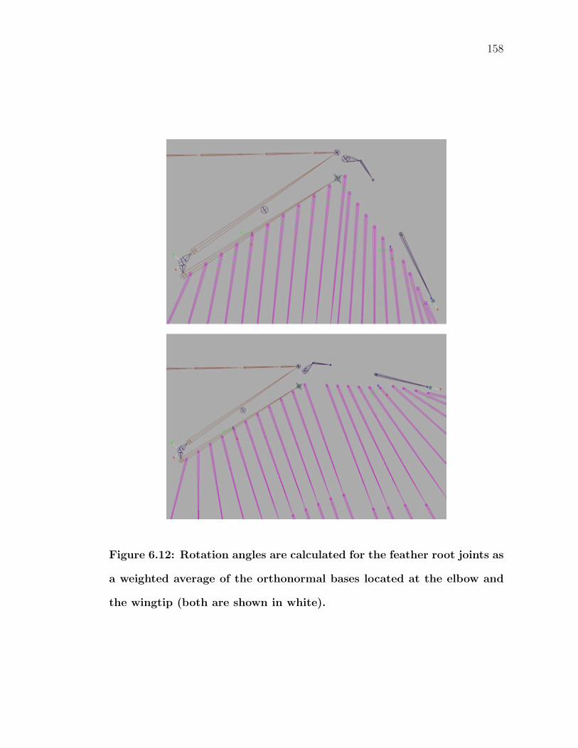
158

Figure 6.12: Rotation angles are calculated for the feather root joints as

a weighted average of the orthonormal bases located at the elbow and

the wingtip (both are shown in white).

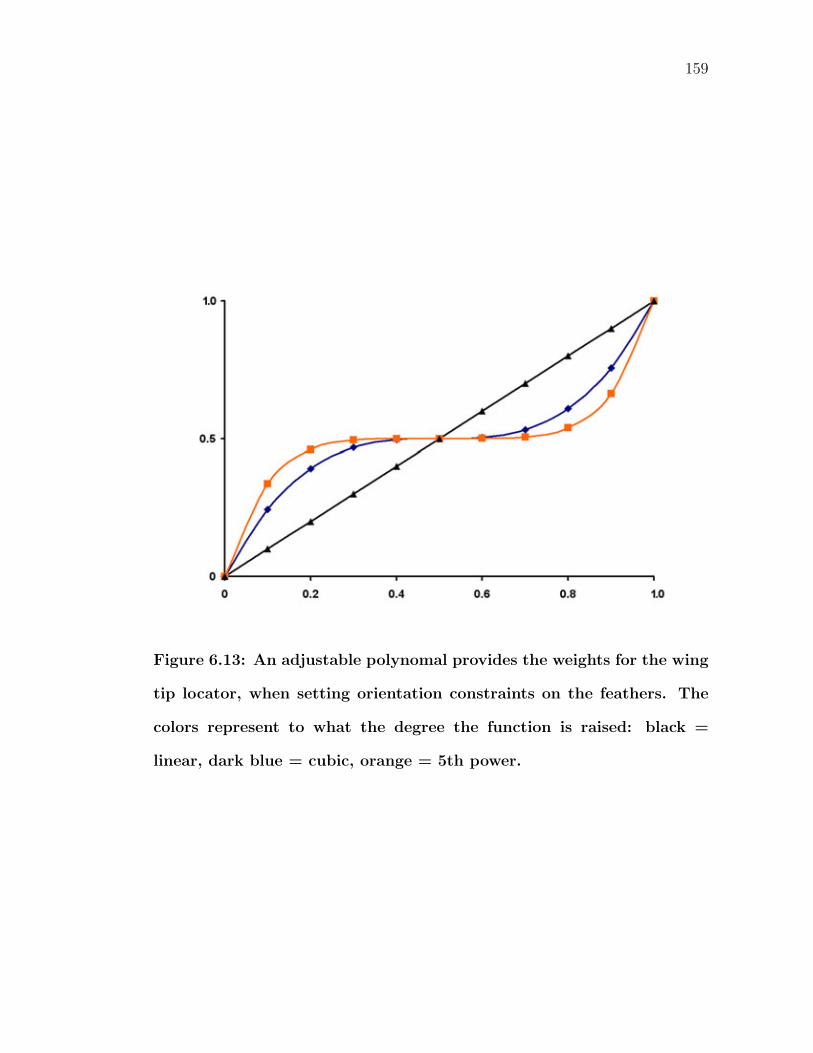
159

Figure 6.13: An adjustable polynomal provides the weights for the wing

tip locator, when setting orientation constraints on the feathers. The

colors represent to what the degree the function is raised: black =

linear, dark blue = cubic, orange = 5th power.

160

to one, essentially reducing Equation 6.4 to y = x + b. However, this failed to

spread the distal primaries sufficiently apart; thus we raise the primaries to the

third power.

As shown in Equation 6.4, normalized Gaussian noise can also be added to

prevent the distribution of feathers from looking too regular. For even richer,

organic-looking animation, key frames can also be set on the noise attribute to

vary the amplitude applied.

Since weighted averages of orthonormal matrices are relatively common in com-

puter animation (i.e. smooth skinning), orientation constraints can be hardware-

accelerated, making this approach much faster than any collision detection scheme.

In addition to the feather’s lateral rotation during wing spreading, primaries

also twist during a wingbeat in response to air resistance, as explained in Chap-

ter 2.5.2. This phenomena is recreated by rotating the twist joint, described earlier

in this chapter, on an axis parallel to the length of the bone. To coordinate the

rotation of several joints, Maya’s driven keys functionality can be used. Driven

keys map one or more attributes to a single attribute. This mapping can be set us-

ing the same key frame interpolation techniques that are ordinarily used to specify

motion with respect to time. Two key frames are used on each feather’s twist joint,

with simple linear interpolation occurring between them, linking them to an twist

attribute for all of the primaries on a wing. The first key frame maps a value of

zero to the twist joints and the twist attribute. The rotation value for the second

key frame is calculated using a polynomial function, such that the amount of twist

dramatically increases distally. With these calculated amounts mapped to a value

of one for the twist attribute, keyframes can then be set on the twist attribute

to control the amount of deformation in a wing’s primaries. As also discussed in

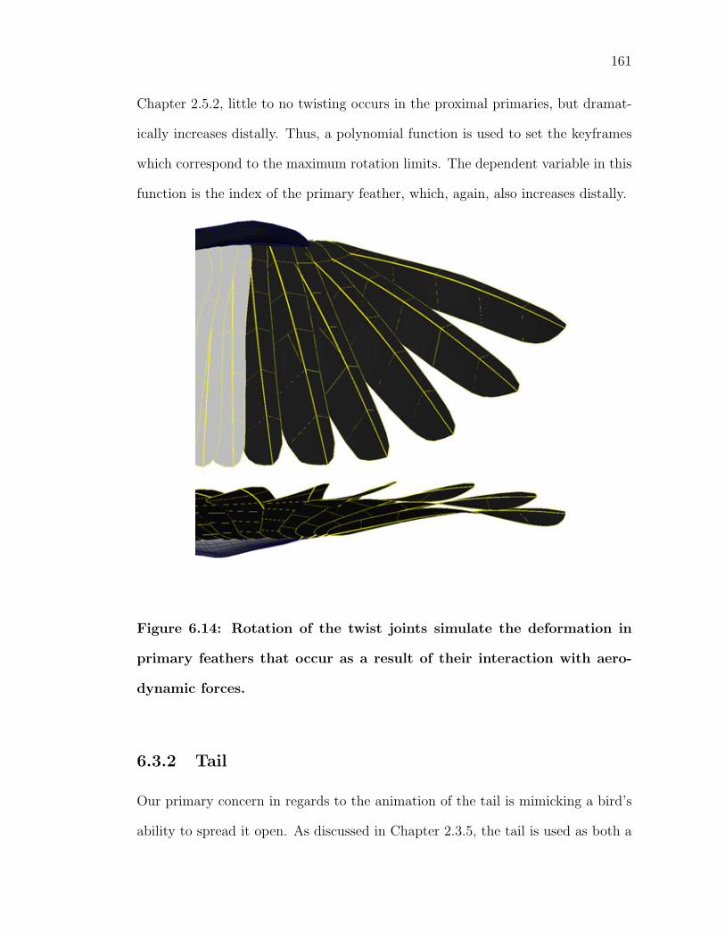
161

Chapter 2.5.2, little to no twisting occurs in the proximal primaries, but dramat-

ically increases distally. Thus, a polynomial function is used to set the keyframes

which correspond to the maximum rotation limits. The dependent variable in this

function is the index of the primary feather, which, again, also increases distally.

Figure 6.14: Rotation of the twist joints simulate the deformation in

primary feathers that occur as a result of their interaction with aero-

dynamic forces.

6.3.2 Tail

Our primary concern in regards to the animation of the tail is mimicking a bird’s

ability to spread it open. As discussed in Chapter 2.3.5, the tail is used as both a

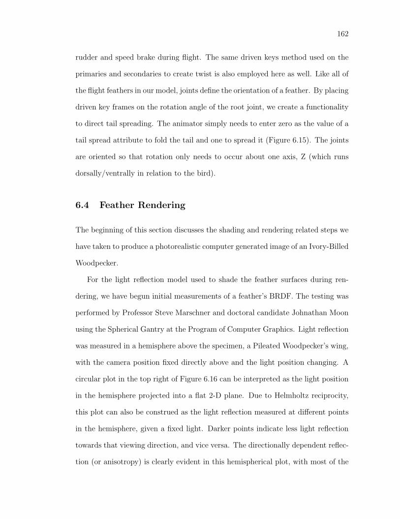
162

rudder and speed brake during flight. The same driven keys method used on the

primaries and secondaries to create twist is also employed here as well. Like all of

the flight feathers in our model, joints define the orientation of a feather. By placing

driven key frames on the rotation angle of the root joint, we create a functionality

to direct tail spreading. The animator simply needs to enter zero as the value of a

tail spread attribute to fold the tail and one to spread it (Figure 6.15). The joints

are oriented so that rotation only needs to occur about one axis, Z (which runs

dorsally/ventrally in relation to the bird).

6.4 Feather Rendering

The beginning of this section discusses the shading and rendering related steps we

have taken to produce a photorealistic computer generated image of an Ivory-Billed

Woodpecker.

For the light reflection model used to shade the feather surfaces during ren-

dering, we have begun initial measurements of a feather’s BRDF. The testing was

performed by Professor Steve Marschner and doctoral candidate Johnathan Moon

using the Spherical Gantry at the Program of Computer Graphics. Light reflection

was measured in a hemisphere above the specimen, a Pileated Woodpecker’s wing,

with the camera position fixed directly above and the light position changing. A

circular plot in the top right of Figure 6.16 can be interpreted as the light position

in the hemisphere projected into a flat 2-D plane. Due to Helmholtz reciprocity,

this plot can also be construed as the light reflection measured at different points

in the hemisphere, given a fixed light. Darker points indicate less light reflection

towards that viewing direction, and vice versa. The directionally dependent reflec-

tion (or anisotropy) is clearly evident in this hemispherical plot, with most of the

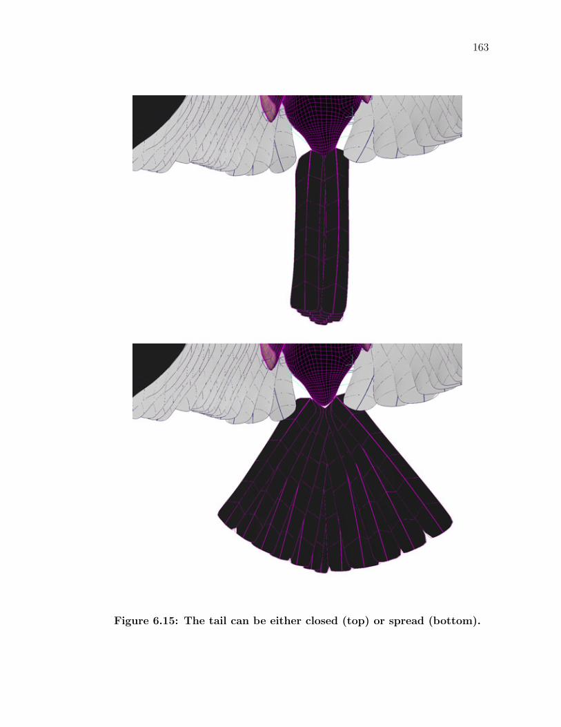
163

Figure 6.15: The tail can be either closed (top) or spread (bottom).

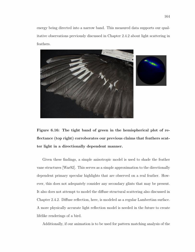
164

energy being directed into a narrow band. This measured data supports our qual-

itative observations previously discussed in Chapter 2.4.2 about light scattering in

feathers.

Figure 6.16: The tight band of green in the hemispherical plot of re-

flectance (top right) corroborates our previous claims that feathers scat-

ter light in a directionally dependent manner.

Given these findings, a simple anisotropic model is used to shade the feather

vane structures [War92]. This serves as a simple approximation to the directionally

dependent primary specular highlights that are observed on a real feather. How-

ever, this does not adequately consider any secondary glints that may be present.

It also does not attempt to model the diffuse structural scattering also discussed in

Chapter 2.4.2. Diffuse reflection, here, is modeled as a regular Lambertian surface.

A more physically accurate light reflection model is needed in the future to create

lifelike renderings of a bird.

Additionally, if our animation is to be used for pattern matching analysis of the

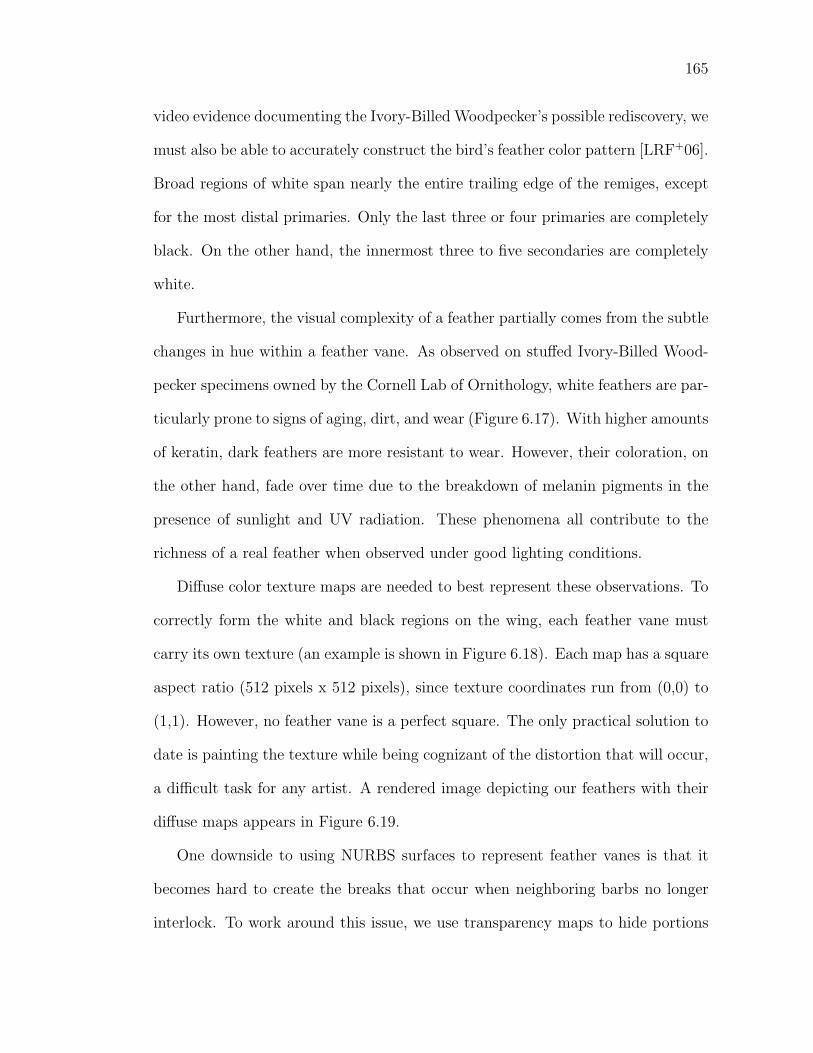
165

video evidence documenting the Ivory-Billed Woodpecker’s possible rediscovery, we

must also be able to accurately construct the bird’s feather color pattern [LRF+06].

Broad regions of white span nearly the entire trailing edge of the remiges, except

for the most distal primaries. Only the last three or four primaries are completely

black. On the other hand, the innermost three to five secondaries are completely

white.

Furthermore, the visual complexity of a feather partially comes from the subtle

changes in hue within a feather vane. As observed on stuffed Ivory-Billed Wood-

pecker specimens owned by the Cornell Lab of Ornithology, white feathers are par-

ticularly prone to signs of aging, dirt, and wear (Figure 6.17). With higher amounts

of keratin, dark feathers are more resistant to wear. However, their coloration, on

the other hand, fade over time due to the breakdown of melanin pigments in the

presence of sunlight and UV radiation. These phenomena all contribute to the

richness of a real feather when observed under good lighting conditions.

Diffuse color texture maps are needed to best represent these observations. To

correctly form the white and black regions on the wing, each feather vane must

carry its own texture (an example is shown in Figure 6.18). Each map has a square

aspect ratio (512 pixels x 512 pixels), since texture coordinates run from (0,0) to

(1,1). However, no feather vane is a perfect square. The only practical solution to

date is painting the texture while being cognizant of the distortion that will occur,

a difficult task for any artist. A rendered image depicting our feathers with their

diffuse maps appears in Figure 6.19.

One downside to using NURBS surfaces to represent feather vanes is that it

becomes hard to create the breaks that occur when neighboring barbs no longer

interlock. To work around this issue, we use transparency maps to hide portions

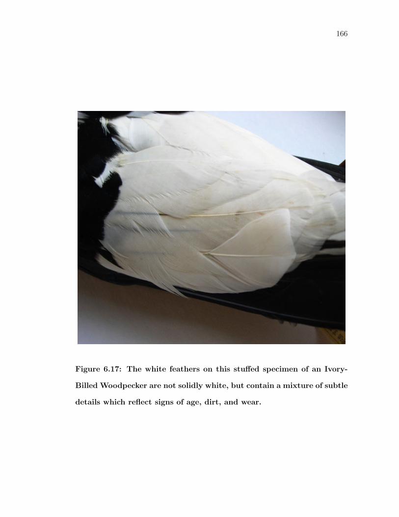
166

Figure 6.17: The white feathers on this stuffed specimen of an Ivory-

Billed Woodpecker are not solidly white, but contain a mixture of subtle

details which reflect signs of age, dirt, and wear.

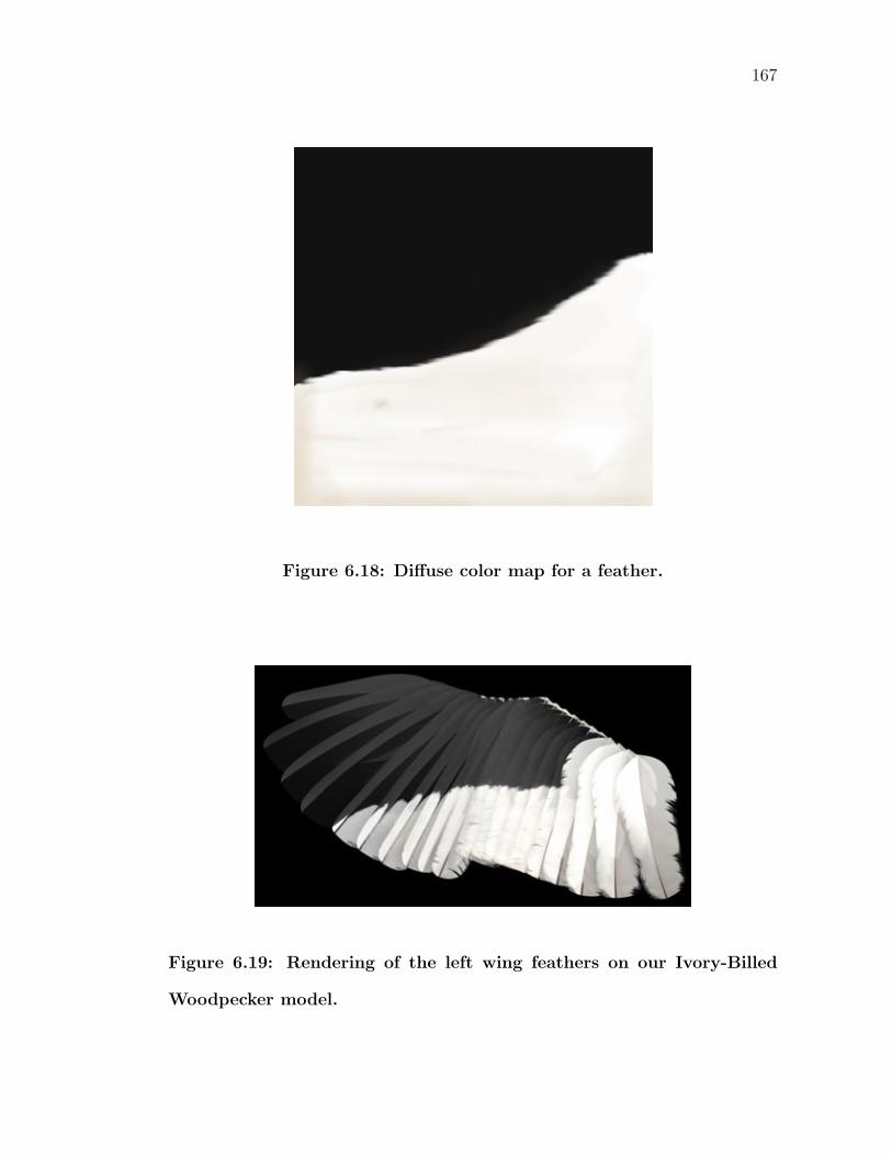
167

Figure 6.18: Diffuse color map for a feather.

Figure 6.19: Rendering of the left wing feathers on our Ivory-Billed

Woodpecker model.

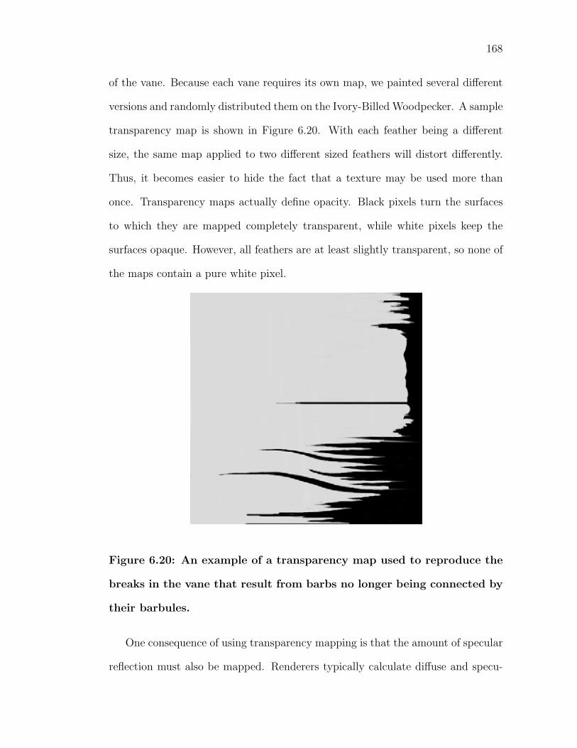
168

of the vane. Because each vane requires its own map, we painted several different

versions and randomly distributed them on the Ivory-Billed Woodpecker. A sample

transparency map is shown in Figure 6.20. With each feather being a different

size, the same map applied to two different sized feathers will distort differently.

Thus, it becomes easier to hide the fact that a texture may be used more than

once. Transparency maps actually define opacity. Black pixels turn the surfaces

to which they are mapped completely transparent, while white pixels keep the

surfaces opaque. However, all feathers are at least slightly transparent, so none of

the maps contain a pure white pixel.

Figure 6.20: An example of a transparency map used to reproduce the

breaks in the vane that result from barbs no longer being connected by

their barbules.

One consequence of using transparency mapping is that the amount of specular

reflection must also be mapped. Renderers typically calculate diffuse and specu-

169

lar color separately. Transparency mapping only removes the diffuse component,

leaving the specular component intact (useful for shiny, transparent objects such

as polished glass). Therefore, for the areas that are completely transparent to

simulate breaks in the feather vane, we also create maps that specify the absence

of specular reflection.

6.4.1 Anti-aliasing and Tessellation

The remainder of this section is dedicated to two key technical issues that arise

when rendering feathers modeled using our approach, anti-aliasing and tessellation.

Careful approaches to each are necessary to produce smooth, high-quality images.

Although they exist as two separate parts of the rendering pipeline, they have the

same effect.

Because of the regular, high-frequency pattern created by the barbs, renderings

become prone to difficult aliasing problems. A term derived from the field of signal

processing, aliasing in the computer graphics domain refers to problems in render-

ing that result from insufficient sampling of the source data [EMP+03, Mar05].

Any computer generated raster image must convert the source data into discrete

pixels through sampling. These samples can later be interpolated to reconstruct

the original continuous signal. When the source data has high frequency changes,

such as with the barbs on feathers, the sampling rate must also be high.

Theoretically, according to the Nyquist theorem, aliasing will occur if the max-

imum frequency in a source function exceeds one half the sampling rate. Since

our barb bump map texture contains very high frequencies, without some sort of

special countermeasure, small-scale features in repeating patterns will create moire

patterns. In fact, our texture represents possibly the worst case scenario for alias-

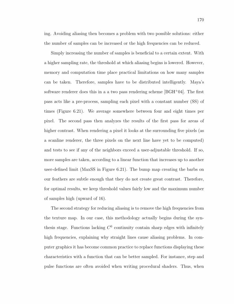
170

ing. Avoiding aliasing then becomes a problem with two possible solutions: either

the number of samples can be increased or the high frequencies can be reduced.

Simply increasing the number of samples is beneficial to a certain extent. With

a higher sampling rate, the threshold at which aliasing begins is lowered. However,

memory and computation time place practical limitations on how many samples

can be taken. Therefore, samples have to be distributed intelligently. Maya’s

software renderer does this in a a two pass rendering scheme [BGH+04]. The first

pass acts like a pre-process, sampling each pixel with a constant number (SS) of

times (Figure 6.21). We average somewhere between four and eight times per

pixel. The second pass then analyzes the results of the first pass for areas of

higher contrast. When rendering a pixel it looks at the surrounding five pixels (as

a scanline renderer, the three pixels on the next line have yet to be computed)

and tests to see if any of the neighbors exceed a user-adjustable threshold. If so,

more samples are taken, according to a linear function that increases up to another

user-defined limit (MaxSS in Figure 6.21). The bump map creating the barbs on

our feathers are subtle enough that they do not create great contrast. Therefore,

for optimal results, we keep threshold values fairly low and the maximum number

of samples high (upward of 16).

The second strategy for reducing aliasing is to remove the high frequencies from

the texture map. In our case, this methodology actually begins during the syn-

thesis stage. Functions lacking C0 continuity contain sharp edges with infinitely

high frequencies, explaining why straight lines cause aliasing problems. In com-

puter graphics it has become common practice to replace functions displaying these

characteristics with a function that can be better sampled. For instance, step and

pulse functions are often avoided when writing procedural shaders. Thus, when

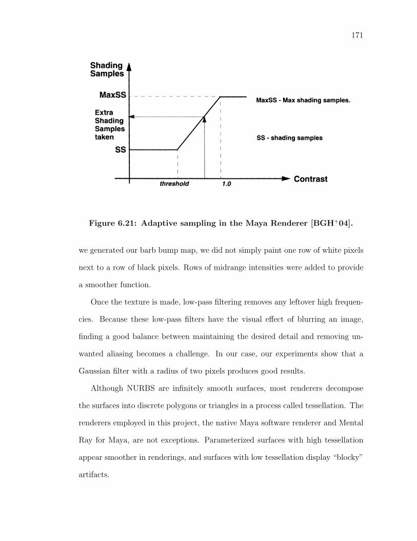
171

Figure 6.21: Adaptive sampling in the Maya Renderer [BGH+04].

we generated our barb bump map, we did not simply paint one row of white pixels

next to a row of black pixels. Rows of midrange intensities were added to provide

a smoother function.

Once the texture is made, low-pass filtering removes any leftover high frequen-

cies. Because these low-pass filters have the visual effect of blurring an image,

finding a good balance between maintaining the desired detail and removing un-

wanted aliasing becomes a challenge. In our case, our experiments show that a

Gaussian filter with a radius of two pixels produces good results.

Although NURBS are infinitely smooth surfaces, most renderers decompose

the surfaces into discrete polygons or triangles in a process called tessellation. The

renderers employed in this project, the native Maya software renderer and Mental

Ray for Maya, are not exceptions. Parameterized surfaces with high tessellation

appear smoother in renderings, and surfaces with low tessellation display “blocky”

artifacts.

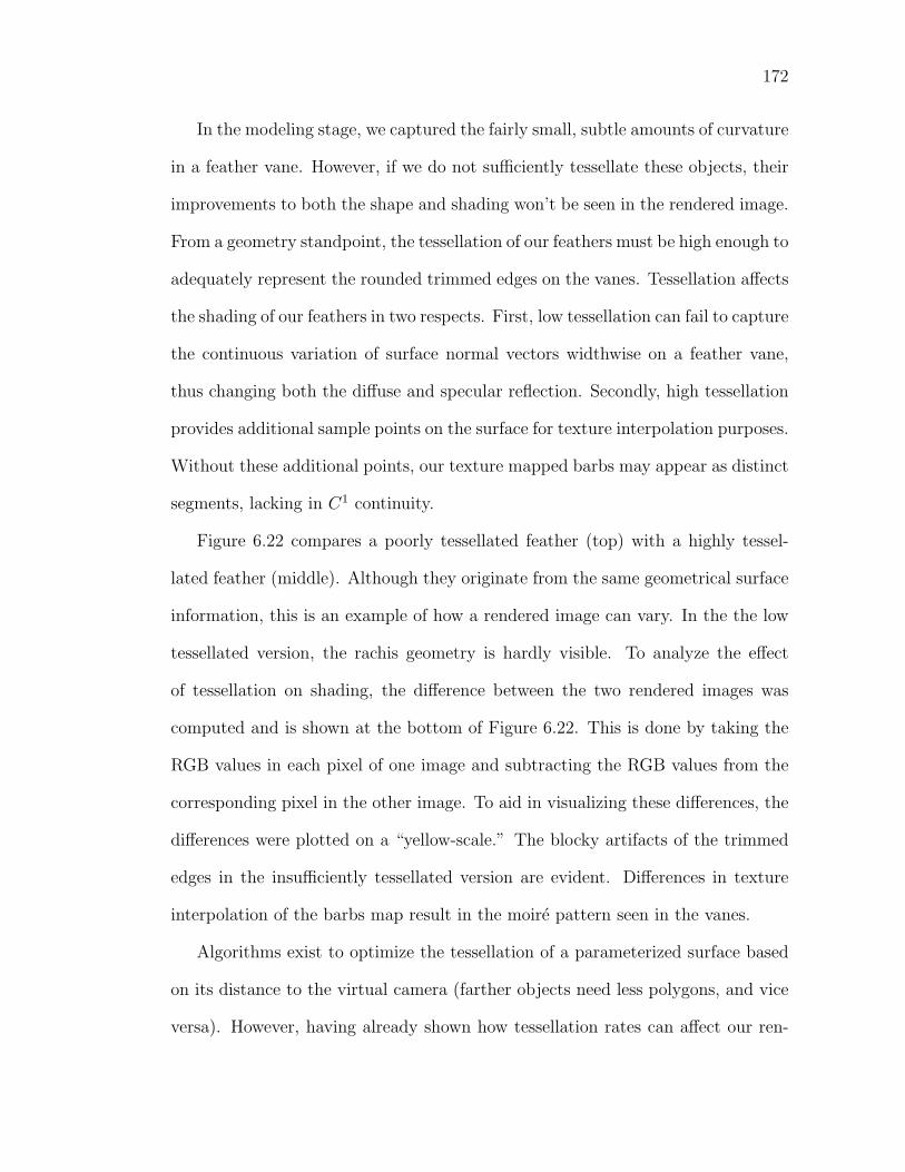
172

In the modeling stage, we captured the fairly small, subtle amounts of curvature

in a feather vane. However, if we do not sufficiently tessellate these objects, their

improvements to both the shape and shading won’t be seen in the rendered image.

From a geometry standpoint, the tessellation of our feathers must be high enough to

adequately represent the rounded trimmed edges on the vanes. Tessellation affects

the shading of our feathers in two respects. First, low tessellation can fail to capture

the continuous variation of surface normal vectors widthwise on a feather vane,

thus changing both the diffuse and specular reflection. Secondly, high tessellation

provides additional sample points on the surface for texture interpolation purposes.

Without these additional points, our texture mapped barbs may appear as distinct

segments, lacking in C1 continuity.

Figure 6.22 compares a poorly tessellated feather (top) with a highly tessel-

lated feather (middle). Although they originate from the same geometrical surface

information, this is an example of how a rendered image can vary. In the the low

tessellated version, the rachis geometry is hardly visible. To analyze the effect

of tessellation on shading, the difference between the two rendered images was

computed and is shown at the bottom of Figure 6.22. This is done by taking the

RGB values in each pixel of one image and subtracting the RGB values from the

corresponding pixel in the other image. To aid in visualizing these differences, the

differences were plotted on a “yellow-scale.” The blocky artifacts of the trimmed

edges in the insufficiently tessellated version are evident. Differences in texture

interpolation of the barbs map result in the moire pattern seen in the vanes.

Algorithms exist to optimize the tessellation of a parameterized surface based

on its distance to the virtual camera (farther objects need less polygons, and vice

versa). However, having already shown how tessellation rates can affect our ren-

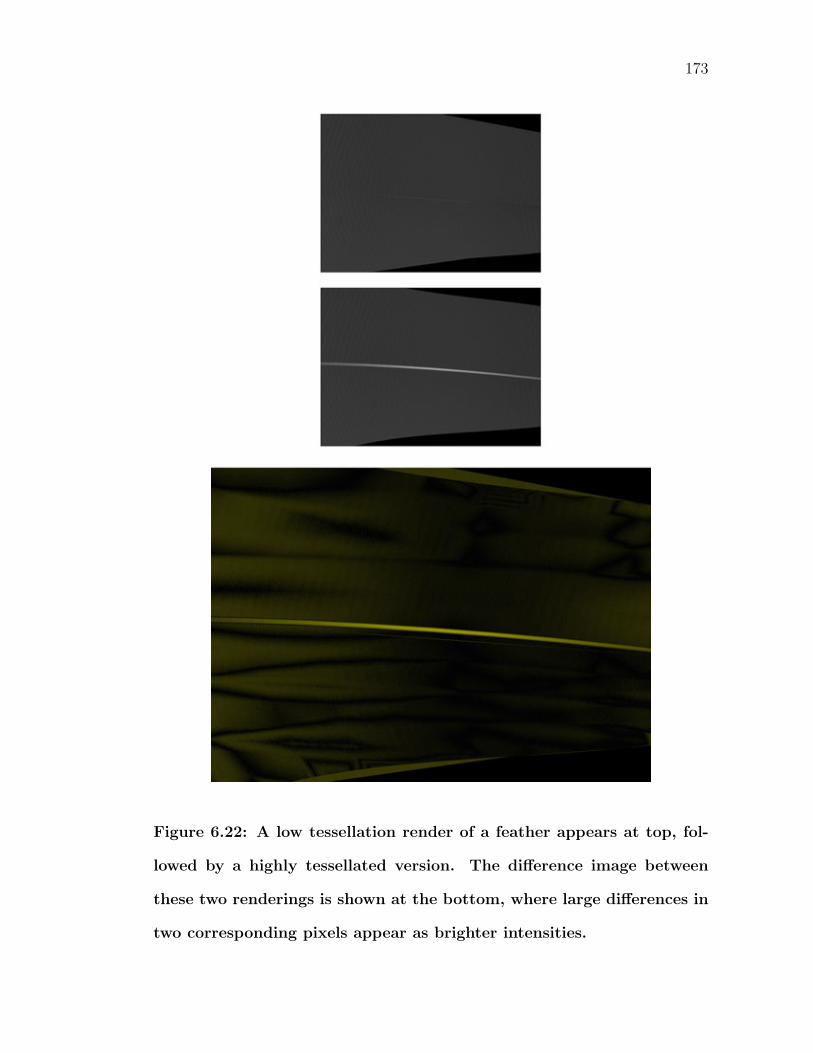
173

Figure 6.22: A low tessellation render of a feather appears at top, fol-

lowed by a highly tessellated version. The difference image between

these two renderings is shown at the bottom, where large differences in

two corresponding pixels appear as brighter intensities.

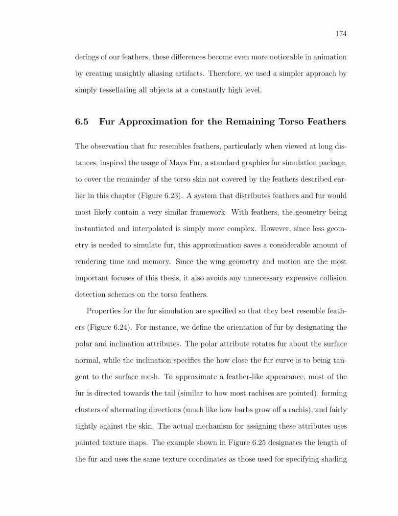
174

derings of our feathers, these differences become even more noticeable in animation

by creating unsightly aliasing artifacts. Therefore, we used a simpler approach by

simply tessellating all objects at a constantly high level.

6.5 Fur Approximation for the Remaining Torso Feathers

The observation that fur resembles feathers, particularly when viewed at long dis-

tances, inspired the usage of Maya Fur, a standard graphics fur simulation package,

to cover the remainder of the torso skin not covered by the feathers described ear-

lier in this chapter (Figure 6.23). A system that distributes feathers and fur would

most likely contain a very similar framework. With feathers, the geometry being

instantiated and interpolated is simply more complex. However, since less geom-

etry is needed to simulate fur, this approximation saves a considerable amount of

rendering time and memory. Since the wing geometry and motion are the most

important focuses of this thesis, it also avoids any unnecessary expensive collision

detection schemes on the torso feathers.

Properties for the fur simulation are specified so that they best resemble feath-

ers (Figure 6.24). For instance, we define the orientation of fur by designating the

polar and inclination attributes. The polar attribute rotates fur about the surface

normal, while the inclination specifies the how close the fur curve is to being tan-

gent to the surface mesh. To approximate a feather-like appearance, most of the

fur is directed towards the tail (similar to how most rachises are pointed), forming

clusters of alternating directions (much like how barbs grow off a rachis), and fairly

tightly against the skin. The actual mechanism for assigning these attributes uses

painted texture maps. The example shown in Figure 6.25 designates the length of

the fur and uses the same texture coordinates as those used for specifying shading

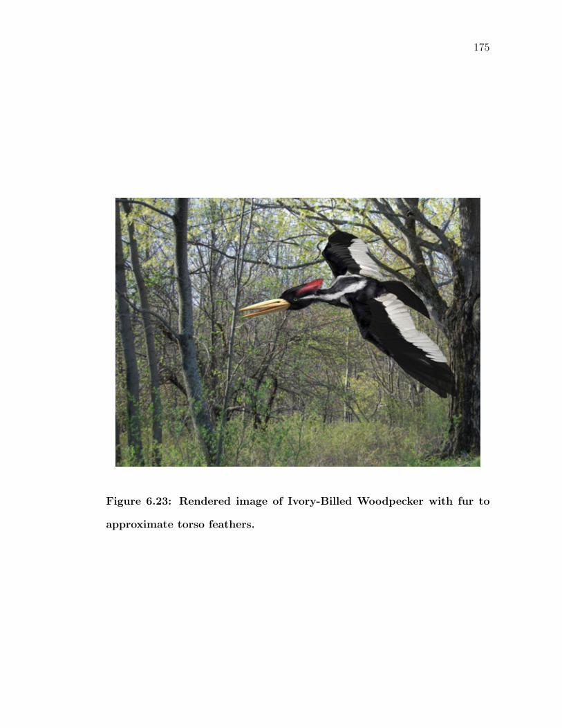
175

Figure 6.23: Rendered image of Ivory-Billed Woodpecker with fur to

approximate torso feathers.

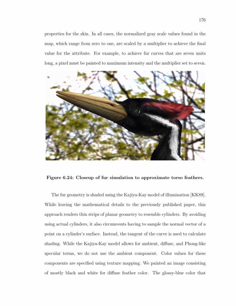
176

properties for the skin. In all cases, the normalized gray scale values found in the

map, which range from zero to one, are scaled by a multiplier to achieve the final

value for the attribute. For example, to achieve fur curves that are seven units

long, a pixel must be painted to maximum intensity and the multiplier set to seven.

Figure 6.24: Closeup of fur simulation to approximate torso feathers.

The fur geometry is shaded using the Kajiya-Kay model of illumination [KK89].

While leaving the mathematical details to the previously published paper, this

approach renders thin strips of planar geometry to resemble cylinders. By avoiding

using actual cylinders, it also circumvents having to sample the normal vector of a

point on a cylinder’s surface. Instead, the tangent of the curve is used to calculate

shading. While the Kajiya-Kay model allows for ambient, diffuse, and Phong-like

specular terms, we do not use the ambient component. Color values for these

components are specified using texture mapping. We painted an image consisting

of mostly black and white for diffuse feather color. The glossy-blue color that

177

Figure 6.25: Attributes for the fur simulation are specified by texture

maps. The map shown above specifies the length of fur.

results from structural coloration is approximated with a broad specular term.

Shadows, including self-shadows, are key contributors to the appearance of

feathers. Since they are not completely opaque and lie in layers, feathers are

analogous to hair, whose self-shadowing importance has been documented. The

interesting effects that occur are evident in Figure 6.26. To duplicate these self-

shadowing effects, we use two separate texture maps, one for the color of the fur

at its base and one at its tip. While the pair do not vary in hue, the intensities of

the base color map are reduced to provide a volumetric effect.

178

Figure 6.26: The importance of self-shadowing to a realistic rendering is

demonstrated above. The image at left is rendered with self-shadowing,

whereas the right one is not [LV00].

CHAPTER 7

CONCLUSION

With somewhere between 8,800-10,000 living species, birds are among the most

diverse class of terrestrial vertebrates and thus raise numerous research questions.

One question that remains popular and unanswered to this day is “How do birds

fly?,” despite being well studied for at least the last thirty years. With so much

variation occurring between species and the need to recreate the most natural

flying environment, answering this question is a difficult task. More recently, the

debate over the validity of the Ivory-Billed Woodpecker’s rediscovery has created

questions of its own. Using our physiologically correct re-creation of the IBW in

this thesis, we anticipate deeper insight to both of these questions.

Our first step towards creating an accurate model of the Ivory-Billed was to

get its geometry correct. While stuffed specimens provide a description of the

feathered exterior, a complete understanding of its internal structure, in particular

the skeleton, is necessary. According to [Dia92], the relative sizes of each bone

in an avian wing determine flying styles for a particular bird during a wingbeat.

For instance, a species with short humerus, radius, and ulna keep their wrist joints

particularly close to the torso and depend on the primary remiges to do most of the

flying work. A pickled specimen of an Ivory-Billed, with its skeleton still intact,

was scanned using high-resolution computer tomography (CT) at the University

of Texas’ DigiMorph Labs. After receiving the volume data, we reconstructed

the specimen using Amira, a high-end commercial visualization software. CT

scans measure material density and map those values to a range of intensities in

a bitmapped image. Thresholds can be placed on these pixel intensity values to

segment specific areas for reconstruction. Contours of the desired target are then

179

180

automatically generated for each two-dimensional slice of the volume data. These

contours are then combined to produce a three-dimensional surface. Two separate

data sets were extracted from the volume data: one of just the skeleton and another

of just the bird’s skin. Due to the negligble difference in density between feather

and skin, significant manual editing of the contours were necessary to remove the

feathers.

Once reconstruction from the CT scan was complete, the data was brought

into Alias’ Maya as reference for our own animated model. The reconstructed

skin model could not be directly used for several reasons: the mesh contained too

many points to be animated in near real-time, was topologically non-manifold, and

had useless interior faces hidden beneath the skin surface. Instead, we used the

reconstructed model to create our own smoothed subdivision surface model.

Feathers that were once deleted from the volume data had to be replaced by

our custom feathers that could be animated along with the skin mesh. The overall

shape of the wing was established by using a model of a Pileated Woodpecker’s

spread wing which had been obtained using a laser-range scanner. For individual

feathers, a user interface was scripted that allowed a user to quickly model flight

feathers for the wings and tail. By specifying only the curvature of the rachis, or

the feather’s central stem, and the outline of the two vanes, the system procedurally

generated the rest of the geometry using NURBS surfaces. Textural bump mapping

provided the appearance of individual barbs. The orientations of the elbow and

major digit were used in a weighted average to determine the orientation of a

remex. Weights were distributed using a polynomial function, forcing the feathers

to spread while minimizing penetration of the neighboring feather. In addition to

the approximately 50 flight feathers, the rest of the contour feathers were generated

181

by Maya’s fur simulation. Although the geometry of a single fur curve does not

quite match the geometry a single real feather, this approximation can be quite

reasonable when the single feather becomes indistinguishable among the hundreds

of real feathers on a bird. Since nearly a million fur follicles were necessary to cover

the entire bird, attributes for the simulation were specified using painted texture

maps.

To date, animation of the Ivory-Billed model was done using traditional keyframe

animation techniques. Joints for the purposes of animating this model were added

by estimating the pivot points of the joints from the imported reconstructed skele-

ton. Ken Dial’s seminal work of a European Starling in a wind tunnel plotted

rotation angles for each joint in the wing as a function of time [DGJ91]. These

angles were used to animate the joints in the wing. Findings from Farish Jenkins’

classic Science paper that described the furcula as a spring during a wingbeat were

incorporated into our animation [JJDGJ88]. This provided secondary motion that

made the bird’s wingbeat appear more natural. Finally, standard smooth skinning

deformed the model.

To truly distinguish our work from simply animation, the laws of physics need to

be implemented in future work. A rigorous recreation of the stretchable patagium

requires knowledge about the elasticity of skin. Preliminary research in computer

graphics have shown that finite element models (FEM) can be used to deform a

character’s skin mesh in real-time [CGC+02, CBC+05]. However, it is uncertain

if the technology is robust enough to handle the challenges presented by thin

flexible membranes. Although the kinematics of a wingbeat are well replicated

in this animation, the actual machinery involved - the musculoskeletal system

- can be more directly integrated. Instead of the arbitrary values used in this

182

thesis, realistic limits on a joint’s range of motion depend on ligaments and bone

structure. Lastly, given the precise representation of a wing, one could calculate

the aerodynamic forces necessary to keep the bird aloft by solving the Navier Stokes

equations. Previous graphics has calculated both the energy produced by and the

deformation of human muscle for a specified motion [TSIF05]; this area of work

could easily be extended to our bird model. Replacing key framed motion with

such data would transform our animation into a tool that would allay some of the

difficultes in avian flight research.

Lastly, we began to measure light reflectance off of a feather using the Spherical

Gantry at Cornell’s Program of Computer Graphics. However, follow up work

has yet to be made on creating a physically-based local illumination model of

light reflection. Reconstituting the mechanisms of structural coloration within the

framework of a photo mapping algorithm would provide photorealistic renderings

of birds. Many of the current scatternig models in computer graphics are based

on Rayleigh and Mie scattering, and would not correctly duplicate the phenomena

which occurs in feathers. From there, pattern matching could be done on the

disputed video footage from the Ivory Billed Woodpecker’s rediscovery if an equally

accurate model of the Pileated Woodpecker was constructed. Other birds could

also be refabricated, opening the door to ornithological parametric studies.

If succesful in these areas, the result becomes a simulation of birds useful to

ornithologists and mechanists alike.

BIBLIOGRAPHY

[BBK94] RE Brown, JJ Baumel, and RD Klemm. Anatomy of the propatagium:The great horned owl (bubo virginiaus). J. Morph., 219:205–224, 1994.

[BBK95] RE Brown, JJ Baumel, and RD Klemm. Mechanics of the avianpropatagium: Flexion-extension mechanism of the avian wing. J.Morph., 225:91–105, 1995.

[BGH+04] C Berndt, P Gheorghian, J Harrington, A Harris, and C McGinnis.Learning Maya 6 — Rendering. Alias Systems, Toronto, Canada,2004.

[BHW96] R Barzel, JF Hughes, and DN Wood. Plausible motion simulationfor computer graphics animation. In Proceedings of the Eurographicsworkshop on Computer animation and simulation ’96, pages 183–197,New York, NY, USA, 1996. Springer-Verlag New York, Inc.

[BM59] WJ Bock and W DeW Miller. The scansorial foot of the woodpeckers,with comments on the evolution of perching and climbing feet in birds.Am. Mus. Novit., 1931(1-45), 1959.

[Bru03] A Bruderlin. A basic hair/fur pipeline. In SIGGRAPH 2003 CourseNotes - Photorealistic Hair Modeling, Animation, and Rendering,2003.

[Bur90] R Burton. Bird Flight: An Illustrated Study of Birds’ Aerial Mastery.Facts on File, New York, NY, USA, 1990.

[BW98] D Baraff and A Witkin. Large steps in cloth simulation. In SIG-GRAPH ’98: Proceedings of the 25th annual conference on Computergraphics and interactive techniques, pages 43–54, New York, NY, USA,1998. ACM Press.

[CB98] WR Corning and AA Biewener. In vivo strains in pigeon flight feathershafts: implications for structural design. J. Exp. Biol., 201:3057–3065, 1998.

[CBC+05] S Capell, M Burkhart, B Curless, T Duchamp, and Z Popovic. Physi-cally based rigging for deformable characters. In SCA ’05: Proceedingsof the 2005 ACM SIGGRAPH/Eurographics symposium on Computeranimation, pages 301–310, New York, NY, USA, 2005. ACM Press.

[CG85] MF Cohen and DP Greenberg. The hemi-cube: a radiosity solution forcomplex environments. In SIGGRAPH ’85: Proceedings of the 12thannual conference on Computer graphics and interactive techniques,pages 31–40, New York, NY, USA, 1985. ACM Press.

183

184

[CGC+02] S Capell, S Green, B Curless, T Duchamp, and Z Popovic. Interactiveskeleton-driven dynamic deformations. In SIGGRAPH ’02: Proceed-ings of the 29th annual conference on Computer graphics and inter-active techniques, pages 586–593, New York, NY, USA, 2002. ACMPress.

[CKH+99] PS Calhoun, BS Kuszyk, DG Heath, JC Carley, and EK Fishman.Three-dimensional volume rendering of spiral ct data: Theory andmethod. Radiographics, 19(3):745–764, 1999.

[CXGS02] Y Chen, Y Xu, B Guo, and HY Shum. Modeling and rendering ofrealistic feathers. ACM Transactions on Graphics (TOG), 21(3):630–636, 2002.

[DCH88] RA Drebin, L Carpenter, and P Hanrahan. Volume rendering. InSIGGRAPH ’88: Proceedings of the 15th annual conference on Com-puter graphics and interactive techniques, pages 65–74, New York, NY,USA, 1988. ACM Press.

[DGJ91] KP Dial, GE Goslow, and FA Jenkins. The functional anatomy ofthe shoulder in the european starling (sturnus vulgaris). J. Morph.,207:327–344, 1991.

[Dia92] KP Dial. Avian forelimb muscles and nonsteady flight: Can birds flywithout using the muscles in their wings? The Auk, 109(4):874–885,1992.

[DKG88] KP Dial, SR Kaplan, and GE Goslow. A functional analysis of theprimary upstroke and downstroke muscles in the domestic pigeon(columbia livia) during flight. J. Exp. Biol., 134:1–16, 1988.

[DKT98] Tony DeRose, Michael Kass, and Tien Truong. Subdivision surfacesin character animation. In SIGGRAPH ’98: Proceedings of the 25thannual conference on Computer graphics and interactive techniques,pages 85–94, New York, NY, USA, 1998. ACM Press.

[DSC95] WK Dai, ZC Shih, and RC Chang. Synthesizing feather textures ingalliformes. In EUROGRAPHICS 95, volume 14, pages 407–420, 1995.

[EDD+95] M Eck, T DeRose, T Duchamp, H Hoppe, M Lounsbery, and W Stuet-zle. Multiresolution analysis of arbitrary meshes. In SIGGRAPH’95: Proceedings of the 22nd annual conference on Computer graphicsand interactive techniques, pages 173–182, New York, NY, USA, 1995.ACM Press.

[EMP+03] DS Ebert, KS Musgrave, D Peachey, K Perlin, and S Worley. Texturingand modeling: a procedural approach. Morgan Kaufmann Publishers,San Francisco, CA, USA, 2003.

185

[FB04] Flesh and Bones. Introduction to ct physics. Website, 2004.http://www.fleshandbones.com/readingroom/pdf/940.pdf.

[FF01] N Foster and R Fedkiw. Practical animation of liquids. In SIGGRAPH’01: Proceedings of the 28th annual conference on Computer graphicsand interactive techniques, pages 23–30, New York, NY, USA, 2001.ACM Press.

[FKU77] H. Fuchs, ZM Kedem, and SP Uselton. Optimal surface reconstructionfrom planar contours. Commun. ACM, 20(10):693–702, 1977.

[FLL+05] JW Fitzpatrick, M Lammertink, MD Luneau, TW Gallagher, BR Har-rison, GR Sparling, KV Rosenberg, RW Rohrbaugh, CH Swarthout,PH Wrege, SB Swarthout, MS Dantzker, RA Charif, TR Barks-dale, JV Remsen, SD Simon, and D Zollner. Ivory-billed woodpecker(campephilus principalis) persists in continental north america. Sci-ence, 308:1460–1462, 2005.

[FM96] N Foster and D Metaxas. Realistic animation of liquids. Graph. ModelsImage Process., 58(5):471–483, 1996.

[Fox76] DL Fox. Animal biochromes and structural colours: physical, chemi-cal, distributional and physiological features of coloured bodies in theanimal world. University of California Press, Berkeley, CA, USA, 1976.

[FW02] CG Franco and M Walter. Modeling and rendering of individual feath-ers. In XV Brazilian Symposium on Computer Graphics and ImageProcessing (SIBGRAPI 02), pages 293–299, 2002.

[Gal05] T Gallagher. The Grail Bird. Houghton Mifflin, Boston, MA, USA,2005.

[GMHP04] K Grochow, SL Martin, A Hertzmann, and Z Popovic. Style-basedinverse kinematics. ACM Trans. Graph., 23(3):522–531, 2004.

[Goo92] D Goodnow. How Birds Fly. Periwinkle Books, Columbia, MD, USA,1992.

[Gra00] FS Grassia. Believable automatically synthesized motion by knowledge-enhanced motion transformation. PhD thesis, CMU Computer Sci-ence, 2000.

[HDD+94] H Hoppe, T DeRose, T Duchamp, M Halstead, H Jin, J McDonald,J Schweitzer, and W Stuetzle. Piecewise smooth surface reconstruc-tion. In SIGGRAPH ’94: Proceedings of the 21st annual conferenceon Computer graphics and interactive techniques, pages 295–302, NewYork, NY, USA, 1994. ACM Press.

186

[HM99] JF Hughes and T M’oller. Building an orthonormal basis from a unitvector. J. Graph. Tools, 4(4):33–35, 1999.

[HWBO95] JK Hodgins, WL Wooten, DC Brogan, and JF O’Brien. Animatinghuman athletics. In SIGGRAPH ’95: Proceedings of the 22nd annualconference on Computer graphics and interactive techniques, pages 71–78, 1995.

[Ima02] Sony Imageworks. Stuart little 2: Taking character animation to thenext level. In SIGGRAPH 2002 Course Notes, 2002.

[JC98] HW Jensen and PH Christensen. Efficient simulation of light trans-port in scences with participating media using photon maps. In SIG-GRAPH ’98: Proceedings of the 25th annual conference on Computergraphics and interactive techniques, pages 311–320, New York, NY,USA, 1998. ACM Press.

[JJDGJ88] FA Jenkins Jr, KP Dial, and GE Goslow Jr. A cineradiographic anal-ysis of bird flight: the wishbone in starlings is a spring. Science,241:1495–1498, 1988.

[JK02] WK Jeong and CH Kim. Direct reconstruction of a displaced subdi-vision surface from unorganized points. Graph. Models, 64(2):78–93,2002.

[Kaj86] JT Kajiya. The rendering equation. In SIGGRAPH ’86: Proceedingsof the 13th annual conference on Computer graphics and interactivetechniques, pages 143–150, New York, NY, USA, 1986. ACM Press.

[KGP02] L Kovar, M Gleicher, and F Pighin. Motion graphs. In SIGGRAPH’02: Proceedings of the 29th annual conference on Computer graphicsand interactive techniques, pages 473–482, New York, NY, USA, 2002.ACM Press.

[KJP02] PG Kry, DL James, and DK Pai. Eigenskin: real time large deforma-tion character skinning in hardware. In SCA ’02: Proceedings of the2002 ACM SIGGRAPH/Eurographics symposium on Computer ani-mation, pages 153–159, New York, NY, USA, 2002. ACM Press.

[KK89] JT Kajiya and TL Kay. Rendering fur with three dimensional tex-tures. In SIGGRAPH ’89: Proceedings of the 16th annual conferenceon Computer graphics and interactive techniques, pages 271–280, NewYork, NY, USA, 1989. ACM Press.

[KL96] V Krishnamurthy and M Levoy. Fitting smooth surfaces to densepolygon meshes. In SIGGRAPH ’96: Proceedings of the 23rd annualconference on Computer graphics and interactive techniques, pages313–324, New York, NY, USA, 1996. ACM Press.

187

[Lan72] MF Land. The physics and biology of animal reflectors. Prog. Biophys.Mol. Biol., 24(77-106), 1972.

[LC87] WE Lorensen and HE Cline. Marching cubes: A high resolution 3dsurface construction algorithm. In SIGGRAPH ’87: Proceedings ofthe 14th annual conference on Computer graphics and interactive tech-niques, pages 163–169, New York, NY, USA, 1987. ACM Press.

[LCF00] JP Lewis, M Cordner, and N Fong. Pose space deformation: a unifiedapproach to shape interpolation and skeleton-driven deformation. InSIGGRAPH ’00: Proceedings of the 27th annual conference on Com-puter graphics and interactive techniques, pages 165–172, New York,NY, USA, 2000. ACM Press/Addison-Wesley Publishing Co.

[Lev88] M Levoy. Display of surfaces from volume data. IEEE Comput. Graph.Appl., 8(3):29–37, 1988.

[LHP05] CK Liu, A Hertzmann, and Z Popovic. Learning physics-based mo-tion style with nonlinear inverse optimization. ACM Transactions onGraphics (TOG), 24(3):1071–1081, 2005.

[LRF+06] M Lammertink, KV Rosenberg, JW Fitzpatrick, MD Luneau,TW Gallagher, and MS Dantzker. Detailed analysis of the video ofa large woodpecker (the ”luneau video”) obtained at cache river na-tional wildlife refuge, arkansas, on 25 april 2004. Technical report,Cornell Laboratory of Ornithology, Ithaca, NY, USA, 2006.

[LS72] AM Lucas and PR Stettenheim. Avian anatomy – integument. USDepartment of Agriculture, Washington DC, USA, 1972.

[LV00] T Lokovic and E Veach. Deep shadow maps. In SIGGRAPH ’00: Pro-ceedings of the 27th annual conference on Computer graphics and in-teractive techniques, pages 385–392, New York, NY, USA, 2000. ACMPress/Addison-Wesley Publishing Co.

[Mar90] EJ Marey. Le vol des oiseaux. Masson, G, Paris, 1890.

[Mar04] C Maraffi. Maya Character Creation: Modeling and animation con-trols. New Riders Publishing, 2004.

[Mar05] SR Marschner. Fundamentals of Computer Graphics, chapter SignalProcessing, pages 71–118. AK Peters, Wellesley, MA, USA, 2005.

[MG03] A Mohr and M Gleicher. Building efficient, accurate character skinsfrom examples. ACM Trans. Graph., 22(3):562–568, 2003.

188

[MGR00] S Marschner, B Guneter, and S Raghupathy. Modeling and render-ing for realistic facial animation. In 11th Eurographics Workshop onRendering, pages 231–242, 2000.

[MJC+03] SR Marschner, HW Jensen, M Cammarano, S Worley, and P Han-rahan. Light scattering from human fibers. ACM Transactions onGraphics (TOG), 22(3):780–791, 2003.

[MSS92] D Meyers, S Skinner, and K Sloan. Surfaces from contours. ACMTrans. Graph., 11(3):228–258, 1992.

[MSW05] KJ McGraw, RJ Safran, and K Wakamatsu. How feather colour re-flects its melanin content. Funct. Ecol., 19:816–821, 2005.

[MTPS04] A McNamara, A Treuille, Z Popovic, and J Stam. Fluid controlusing the adjoint method. ACM Transactions on Graphics (TOG),23(3):449–456, 2004.

[Nor90] UM Norberg. Vertebrate Flight. Springer-Verlag, Berlin, Germany,1990.

[PAT03] RO Prum, S Andersson, and RH Torres. Coherent scattering of ultra-violet light by avian feather barbs. The Auk, 120:163–170, 2003.

[Pen89] CJ Pennychuick. Bird Flight Performance. Oxford University Press,Oxford, England, 1989.

[PL90] P Prusinkiewicz and A Lindenmayer. The Algorithmic Beauty ofPlants. Springer-Verlag New York, Inc., New York, NY, USA, 1990.

[PL93] NS Proctor and PJ Lynch. Manual of Ornithology: Avian Structureand Function. Yale University Press, New Haven and London, 1993.

[PRB04] S Podulka, RW Rohrbaugh, and R Bonney, editors. Handbook of BirdBiology. Princeton University Press, Ithaca, NY, USA, 2004.

[PSHG97a] SO Poore, A Sanchez-Haiman, and GE Goslow. The contractile prop-erties of the m. supracoracoideus in the pigeon and starling: a case forlong-axis rotation of the humerus. J. Exp. Biol., 200:2987–3002, 1997.

[PSHG97b] SO Poore, A Sanchez-Haiman, and GE Goslow. Wing upstroke andthe evolution of flapping flight. Nature, 387(6635):799–802, 1997.

[PT97] L Piegl and W Tiller. The NURBS book. Springer-Verlag, New York,NY, 1997.

[PT03] RO Prum and RH Torres. Fourier tool for the analysis of coherentlight scattering by bio-optical nanostructures. Integr. Comp. Biol.,43:591–602, 2003.

189

[PTWD98] RO Prum, RH Torres, S Williamson, and J Dyck. Coherent lightscattering by blue feather barbs. Nature, 396:28–29, 1998.

[PTWD99] RO Prum, RH Torres, S Williamson, and J Dyck. Two-dimensionalfourier analysis of the spongy medullary keratin of structurallycoloured feather barbs. Proc. R. Soc. Lond., 266:13–22, 1999.

[Rai85] RJ Raikow. Form and Function in Birds, chapter Locomotor System,pages 57–147. Academic Press, London, England, 1985.

[RW99] B Ramakrishnananda and KC Wong. Animating bird flight usingaerodynamics. The Visual Computer, 15:494–508, 1999.

[SASW96] V Spitzer, MJ Ackerman, AL Scherzinger, and D Whitlock. The visiblehuman male: a technical report. J Am Med Inform Assoc, 3(2):118–130, 1996.

[SFF91] MR Stytz, G Frieder, and O Frieder. Three-dimensional medicalimaging: algorithms and computer systems. ACM Comput. Surv.,23(4):421–499, 1991.

[SH85] RIC Spearman and JA Hardy. Form and Function in Birds, chapterIntegument, pages 1–56. Academic Press, Orlando, FL, USA, 1985.

[SH02] L Streit and W Heidrich. A biologically-parameterized feather model.In EUROGRAPHICS 2002, volume 21, 2002.

[Sim63] K Simkiss. Bird Flight. Hutchinson Educational, London, England,1963.

[SM00] J. Shi and J. Malik. Normalized cuts and image segmentation.IEEE Transactions on Pattern Analysis and Machine Intelligence,22(8):888–905, 2000.

[Soc05] Stanislaus Audubon Society. Highlights of species observed. Web-site, 2005. http://www.stanislausbirds.org/BY2004/cvby–species–seen.htm.

[Sof03] Template Graphics Software. Amira 3.1 user’s guide and manual.Website, 2003. http://www.amiravis.com/Amira31-manual.pdf.

[SSAC88] PK Sahoo, S Soltani, Wong. AKC, and YC Chen. A survey of thresh-olding techniques. Comput. Vision Graph. Image Process., 41(2):233–260, 1988.

[SW98] V Spitzer and D Whitlock. The visible human dataset: The anatomicalplatform for human simulation. Anat Rec, 253(2):49–57, 1998.

190

[Tan42] JT Tanner. The Ivory-billed Woodpecker. Natl. Audubon Society, NewYork, NY, USA, 1942.

[TD96] BW Tobalske and KP Dial. Flight kinematics of black-billed magpiesand pigeons over a wide range of speeds. J. Exp. Biol., 199:263–280,1996.

[Ten96] H Tennekes. The Simple Science of Flight: From Insects to JumboJets. MIT Press, Cambridge, MA, USA, 1996.

[TFM03] Chicago The Field Museum. Specimen preparation:Pickling, stuffing, boiling, and bugs. Website, 2003.http://www.fieldmuseum.org/expeditions/stanley/about3.html.

[Tic03] WLN Tickell. White plumage. Waterbirds, 26:1–12, 2003.

[TMPS03] A Treuille, A McNamara, Z Popovic, and J Stam. Keyframe con-trol of smoke simulations. ACM Transactions on Graphics (TOG),22(3):716–723, 2003.

[Tob00] BW Tobalske. Biomechanics and physiology of gait selection in flyingbirds. Physiological and Biochemical Zoology, 73:736–750, 2000.

[TSIF05] J Teran, E Sifakis, G Irving, and R Fedkiw. Robust quasistatic finiteelements and flesh simulation. In SCA ’05: Proceedings of the 2005ACM SIGGRAPH/Eurographics symposium on Computer animation,pages 181–190, New York, NY, USA, 2005. ACM Press.

[Tur92] G Turk. Re-tiling polygonal surfaces. In SIGGRAPH ’92: Proceedingsof the 19th annual conference on Computer graphics and interactivetechniques, pages 55–64, New York, NY, USA, 1992. ACM Press.

[Vaz94] RJ Vazquez. The automating skeletal and muscular mechanisms ofthe avian wing (aves). Zoomorphology, 114:59–71, 1994.

[Vid05] JJ Videler. Avian flight. Oxford University Press, Oxford, England,2005.

[War92] GJ Ward. Measuring and modeling anisotropic reflection. In SIG-GRAPH ’92: Proceedings of the 19th annual conference on Computergraphics and interactive techniques, pages 265–272, New York, NY,USA, 1992. ACM Press.

[WH94] AP Witkin and PS Heckbert. Using particles to sample and con-trol implicit surfaces. In SIGGRAPH ’94: Proceedings of the 21stannual conference on Computer graphics and interactive techniques,pages 269–277, 1994.

191

[WP03] J Wu and Z Popovic. Realistic modeling of bird flight animations. InACM Transactions on Graphics (TOG), pages 888–895, 2003.

[WS84] AJ Ward-Smith. Biophysical Aerodynamics and the Natural Environ-ment. John Wiley and Sons, Chichester, England, 1984.

[ZB94] J Zhao and NI Badler. Inverse kinematics positioning using nonlin-ear programming for highly articulated figures. ACM Trans. Graph.,13(4):313–336, 1994.