Embed Size (px)
Citation preview
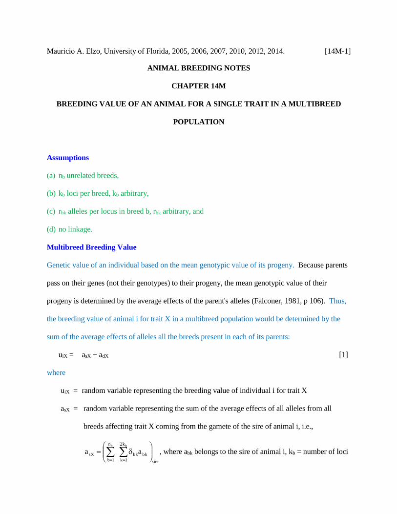
Mauricio A. Elzo, University of Florida, 2005, 2006, 2007, 2010, 2012, 2014. [14M-1]
ANIMAL BREEDING NOTES
CHAPTER 14M
BREEDING VALUE OF AN ANIMAL FOR A SINGLE TRAIT IN A MULTIBREED
POPULATION
Assumptions
(a) nb unrelated breeds,
(b) kb loci per breed, kb arbitrary,
(c) rbk alleles per locus in breed b, rbk arbitrary, and
(d) no linkage.
Multibreed Breeding Value
Genetic value of an individual based on the mean genotypic value of its progeny. Because parents
pass on their genes (not their genotypes) to their progeny, the mean genotypic value of their
progeny is determined by the average effects of the parent's alleles (Falconer, 1981, p 106). Thus,
the breeding value of animal i for trait X in a multibreed population would be determined by the
sum of the average effects of alleles all the breeds present in each of its parents:
uiX = asX + adX [1]
where
uiX = random variable representing the breeding value of individual i for trait X
asX = random variable representing the sum of the average effects of all alleles from all
breeds affecting trait X coming from the gamete of the sire of animal i, i.e.,
sire
k2
1k
bkbk
n
1b
sX
bb
aa
, where abk belongs to the sire of animal i, kb = number of loci
Mauricio A. Elzo, University of Florida, 2005, 2006, 2007, 2010, 2012, 2014. [14M-2]
in breed b, and δbk is a Kronecker delta, i.e., δbk = 0 or 1; δbk will be zero (2kb/2) times
and one (2kb/2) times, because a random sample of only 2 of the male alleles from
each breed is expected to be passed on to individual i.
adX = random variable representing the sum of the average effects of all alleles affecting a
trait, coming from the gamete of the dam of animal i, i.e.,
dam
k2
1k
bkbk
n
1b
dX
bb
aa
, where abk belongs to the dam of animal i.
Average genetic effects are defined as deviations from the average gene at each locus within
each breed; thus, the expected value of uiX is:
E[uiX] = ]aa[E dXsX
= ]a[E]a[E dXsX
=
dam
k2
1k
bkbk
n
1bsire
k2
1k
bkbk
n
1b
bbbb
aEaE
=
dam
k2
1k
bkbk
n
1bsire
k2
1k
bkbk
n
1b
bbbb
b,k|aEb,k|aE
= 0 + 0
= 0
The variance of uiX is:
var(uiX) = var(asX + adX)
= var(asX) + var(adX) + 2 cov(asX,adX)
The covariance between the breeding values of animal i for traits X and Z is:
cov(uiX, uiZ) = cov(asX + adX, asZ + adZ)
Mauricio A. Elzo, University of Florida, 2005, 2006, 2007, 2010, 2012, 2014. [14M-3]
= cov(asX, asZ) + cov(asX, adZ) + cov(adX, asZ) + cov(adX, adZ)
By conditioning on the breeding values of the sire (usX) and the dam (udX) of animal i, var(uiX)
becomes:
var(uiX) = var(E[asX│usX]) + E[var(asX│usX)]
+ var(E(adX│udX]) + E[var(adX│udX)]
+ 2 cov(E[asX│usX], E[adX│udX])
+ 2 E[cov(asX│usX, adX│udX)]
But asX is the average effect of 2 of the alleles affecting the trait in the sire, i.e., asX = 2 usX.
Thus,
E[asX│usX] = E[2 usX│usX]
= 2 usX
Applying a similar argument to adX yields:
E[adX│udX] = 2 udX
Thus, for the sire of animal i,
var(E[asX│usX]) = var(2 usX)
= 3 var(usX)
=
cs
2
AX
n
1ccsds,ss2
1s
2
AX41
cs
a
=
cs
2
AX
n
1c
css
2
AX41
cs
F
(= 3 (σA2 + Fs σA
2) in a single breed population)
where
ncs = number of common ancestors for sire s
Mauricio A. Elzo, University of Florida, 2005, 2006, 2007, 2010, 2012, 2014. [14M-4]
csds,ssa = additive relationship between the sire and the dam of sire
s through common ancestor c
s
2
AX = multibreed additive genetic variance for trait X of the
sire
cs
2
AX = multibreed additive genetic variance for trait X of the
common ancestor of the sire and dam of sire s and, for
the dam of animal i,
Similarly, for the dam of animal i,
var(E[adX│udX]) =
cd
2
AX
n
1ccddd,sd2
1d
2
AX41
cd
a
=
cd
2
AX
n
1c
cdd
2
AX41
cd
F
(= 3 (σA2 + Fd σA
2) in a single breed population)
What is E[var(asX│usX)]?
E[var(asX│usX)] = var (asX) B var(E[asX│usX])
Here,
var(asX) =
sire
k2
1k
bkbk
n
1b
bb
avar
Also, by definition,
bb k2
1k
bk
n
1b
avar = σAX2 = multibreed additive genetic variance for trait X.
An expression for the multibreed additive genetic variance for trait X can be obtained by
Mauricio A. Elzo, University of Florida, 2005, 2006, 2007, 2010, 2012, 2014. [14M-5]
conditioning on the breed of origin of alleles as follows:
σAX2 = ])b|X[Evar(]b|X[var(E
σAX2 =
'bb
2
aX
n
b'b
d
'b
d
b
s
'b
s
b
n
1b
1n
1bb
2
aX
i
b
bb b
)pppp(p
where superscripts i, s and d correspond to animal, sire and dam, subscripts b and b represent
two breeds, and
nb = number of breeds
pbx = expected fraction of breed b in animal x, x = i, s, d
(σaX2)b = additive intrabreed variance of trait X for breed b
(σaX2)bb = additive interbreed variance of trait X for the pair of breeds b and b
Thus, for the sire of animal i,
var(asX) =
sire
k2
1k
bkbk
n
1b
bb
avar
= 2 (σAX2)s
and
E[var(asX│usX)] =
cs
2
AX
n
1ccsds,ss2
1s
2
AX41
s
2
AX21
cs
a
=
cs
2
AX
n
1ccsds,ss2
1s
2
AX41
cs
a
=
cs
2
AX
n
1c
css
2
AX41
cs
F
(= 3 (σA2 B Fs σA
2) in a single breed population)
Similarly, for the dam of animal i,
Mauricio A. Elzo, University of Florida, 2005, 2006, 2007, 2010, 2012, 2014. [14M-6]
var(adX) =
dam
k2
1k
bkbk
n
1b
bb
avar
= 2 (σAX2)d
and
E[var(adX│udX)] =
cd
2
AX
n
1ccddd,sd2
1d
2
AX41
d
2
AX21
cd
a
=
cd
2
AX
n
1ccddd,sd2
1d
2
AX41
cd
a
=
cd
2
AX
n
1c
cdd
2
AX41
cd
F
(= 3 (σA2 B Fd σA
2) in a single breed population)
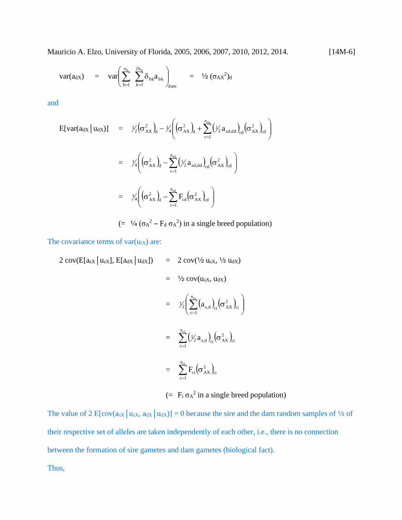
The covariance terms of var(uiX) are:
2 cov(E[asX│usX], E[adX│udX]) = 2 cov(2 usX, 2 udX)
= 2 cov(usX, udX)
=
ci
2
AX
n
1ccid,s2
1
ci
a
= ci
2
AX
n
1ccid,s2
1
ci
a
= ci
2
AX
n
1c
ci
ci
F
(= Fi σA2 in a single breed population)
The value of 2 E[cov(asX│usX, adX│udX)] = 0 because the sire and the dam random samples of 2 of
their respective set of alleles are taken independently of each other, i.e., there is no connection
between the formation of sire gametes and dam gametes (biological fact).
Thus,
Mauricio A. Elzo, University of Florida, 2005, 2006, 2007, 2010, 2012, 2014. [14M-7]
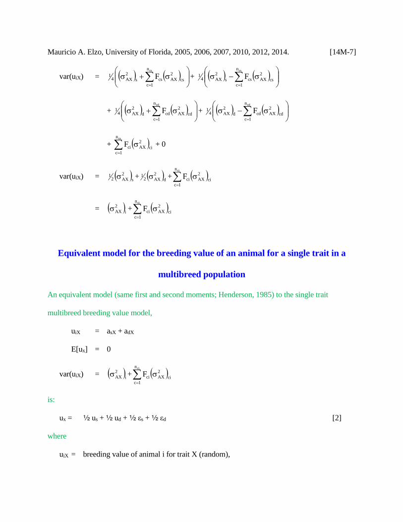
var(uiX) =
cs
2
AX
n
1c
css
2
AX41
cs
F +
cs
2
AX
n
1c
css
2
AX41
cs
F
+
cd
2
AX
n
1c
cdd
2
AX41
cd
F +
cd
2
AX
n
1c
cdd
2
AX41
cd
F
+ ci
2
AX
n
1c
ci
cs
F
+ 0
var(uiX) = s
2
AX21 +
d
2
AX21 +
ci
2
AX
n
1c
ci
ci
F
= i
2
AX + ci
2
AX
n
1c
ci
ci
F
Equivalent model for the breeding value of an animal for a single trait in a
multibreed population
An equivalent model (same first and second moments; Henderson, 1985) to the single trait
multibreed breeding value model,
uiX = asX + adX
E[ux] = 0
var(uiX) = i
2
AX + ci
2
AX
n
1c
ci
ci
F
is:
ux = 2 us + 2 ud + 2 εs + 2 εd [2]
where
uiX = breeding value of animal i for trait X (random),
Mauricio A. Elzo, University of Florida, 2005, 2006, 2007, 2010, 2012, 2014. [14M-8]
usX = breeding value of sire s for trait X (random),
udX = breeding value of dam d for trait X (random),
εsX = Mendelian sampling occurring during gametogenesis in sire s for trait X (random),
εdX = Mendelian sampling in dam d for trait X (random).
The Mendelian sampling terms εsX and εdX are independent of each other and independent from
breeding values. All random variables have expected values equal to zero, i.e.,
E[uiX] = 0
and
var(uiX) = var(2 usX + 2 udX) + var(2 εsX) + var(2 εdX)
where
var(2 usX + 2 udX) = var(2 usX) + var(2 udX) + 2 cov(2 usX, 2 udX)
=
cs
2
AX
n
1c
css
2
AX41
cs
F +
cd
2
AX
n
1c
cdd
2
AX41
cd
F
+ ci
2
AX
n
1c
ci
cs
F
(= 3 (1 + Fs) σA2 + 3 (1 +Fd) σA
2 + Fx σA2 in a single breed
population)
Because the sampling process during gamete formation (Mendelian sampling) in the male and
female gametes is completely independent of each other, any loss of variation during this process
would be due to (i) inbreeding in the male present in the male gamete, and (ii) inbreeding in the
female present in the female gamete. Thus,
var(2 εsX) =
cs
2
AX
n
1c
cs41
s
2
AX41
cs
F
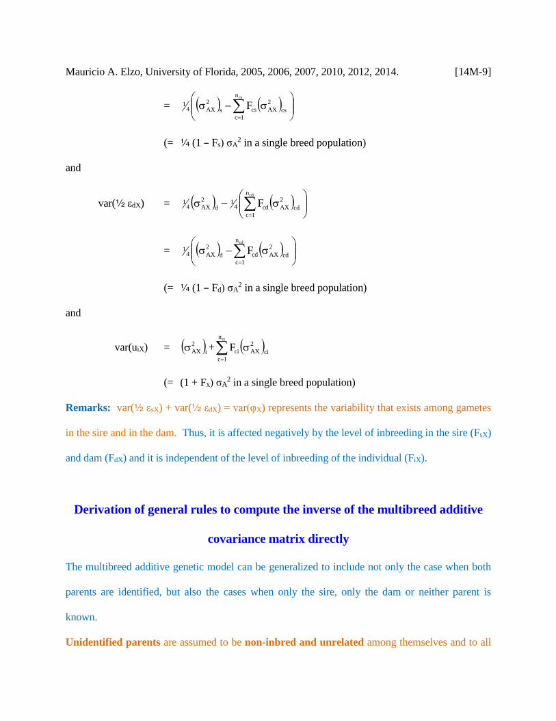
Mauricio A. Elzo, University of Florida, 2005, 2006, 2007, 2010, 2012, 2014. [14M-9]
=
cs
2
AX
n
1c
css
2
AX41
cs
F
(= 3 (1 B Fs) σA2 in a single breed population)
and
var(2 εdX) =
cd
2
AX
n
1c
cd41
d
2
AX41
cd
F
=
cd
2
AX
n
1c
cdd
2
AX41
cd
F
(= 3 (1 B Fd) σA2 in a single breed population)
and
var(uiX) = i
2
AX + ci
2
AX
n
1c
ci
ci
F
(= (1 + Fx) σA2 in a single breed population)
Remarks: var(2 εsX) + var(2 εdX) = var(φX) represents the variability that exists among gametes
in the sire and in the dam. Thus, it is affected negatively by the level of inbreeding in the sire (FsX)
and dam (FdX) and it is independent of the level of inbreeding of the individual (FiX).
Derivation of general rules to compute the inverse of the multibreed additive
covariance matrix directly
The multibreed additive genetic model can be generalized to include not only the case when both
parents are identified, but also the cases when only the sire, only the dam or neither parent is
known.
Unidentified parents are assumed to be non-inbred and unrelated among themselves and to all
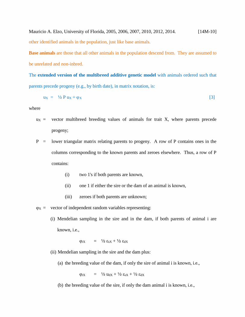
Mauricio A. Elzo, University of Florida, 2005, 2006, 2007, 2010, 2012, 2014. [14M-10]
other identified animals in the population, just like base animals.
Base animals are those that all other animals in the population descend from. They are assumed to
be unrelated and non-inbred.
The extended version of the multibreed additive genetic model with animals ordered such that
parents precede progeny (e.g., by birth date), in matrix notation, is:
uX = 2 P uX + φ X [3]
where
uX = vector multibreed breeding values of animals for trait X, where parents precede
progeny;
P = lower triangular matrix relating parents to progeny. A row of P contains ones in the
columns corresponding to the known parents and zeroes elsewhere. Thus, a row of P
contains:
(i) two 1's if both parents are known,
(ii) one 1 if either the sire or the dam of an animal is known,
(iii) zeroes if both parents are unknown;
φX = vector of independent random variables representing:
(i) Mendelian sampling in the sire and in the dam, if both parents of animal i are
known, i.e.,
φiX = 2 εsX + 2 εdX
(ii) Mendelian sampling in the sire and the dam plus:
(a) the breeding value of the dam, if only the sire of animal i is known, i.e.,
φiX = 2 udX + 2 εsX + 2 εdX
(b) the breeding value of the sire, if only the dam animal i is known, i.e.,
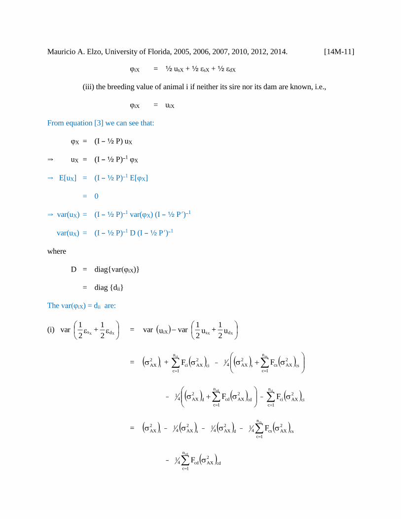
Mauricio A. Elzo, University of Florida, 2005, 2006, 2007, 2010, 2012, 2014. [14M-11]
φiX = 2 usX + 2 εsX + 2 εdX
(iii) the breeding value of animal i if neither its sire nor its dam are known, i.e.,
φiX = uiX
From equation [3] we can see that:
φX = (I B 2 P) uX
uX = (I B 2 P)B1 φX
E[uX] = (I B 2 P)B1 E[φX]
= 0
var(uX) = (I B 2 P)B1 var(φX) (I B 2 P)B1
var(uX) = (I B 2 P)B1 D (I B 2 P)B1
where
D = diag{var(φiX)}
= diag {dii}
The var(φiX) = dii are:
(i)
ds XX 2
1 +
2
1var =
u
2
1 + u
2
1 var uvar dsiX XX
= i
2
AX + ci
2
AX
n
1c
ci
ci
F
-
cs
2
AX
n
1c
css
2
AX41
cs
F
-
cd
2
AX
n
1c
cdd
2
AX41
cd
F - ci
2
AX
n
1c
ci
ci
F
= i
2
AX - s
2
AX41 -
d
2
AX41 -
cs
2
AX
n
1c
cs41
cs
F
- cd
2
AX
n
1c
cd41
cd
F
Mauricio A. Elzo, University of Florida, 2005, 2006, 2007, 2010, 2012, 2014. [14M-12]
if s and d are known
(ii)
dsd XXX
2
1 +
2
1 + u
2
1var =
u
2
1 var uvar siX X
= i
2
AX -
cs
2
AX
n
1c
css
2
AX41
cs
F
= i
2
AX - s
2
AX41 -
cs
2
AX
n
1c
cs41
cs
F
if s is known only
(iii)
dss XXX
2
1 +
2
1 + u
2
1var =
u
2
1 var uvar diX X
= i
2
AX -
cd
2
AX
n
1c
cdd
2
AX41
cd
F
= i
2
AX - d
2
AX41 -
cd
2
AX
n
1c
cd41
cd
F
if d is known only
(iv)
dsds XXXX
2
1 +
2
1 + u
2
1 + u
2
1var = var(uiX)
= i
2
AX
if neither s nor d are known
But
var(uX) =
’ P2
1I D P
2
1I
11
= GAX
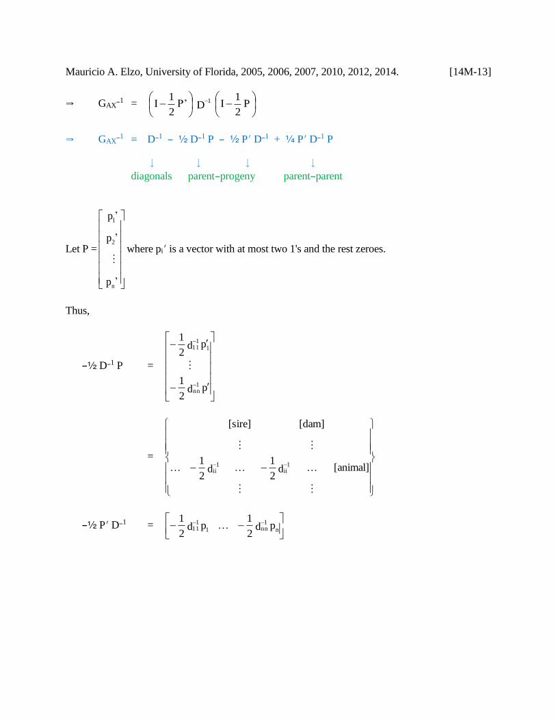
Mauricio A. Elzo, University of Florida, 2005, 2006, 2007, 2010, 2012, 2014. [14M-13]
GAXB1 =
P
2
1I D P’
2
1I 1
GAXB1 = DB1 B 2 DB1 P B 2 P DB1 + 3 P DB1 P
diagonals parentBprogeny parentBparent
Let P =
’p
’p
’p
n
2
1
where pi is a vector with at most two 1's and the rest zeroes.
Thus,
B2 DB1 P =
p d 2
1
p d 2
1
1nn
11
11
=
[animal]d 2
1d
2
1
[dam][sire]
1ii
1ii
B2 P DB1 =
p d
2
1p d
2
1n
1nn1
111
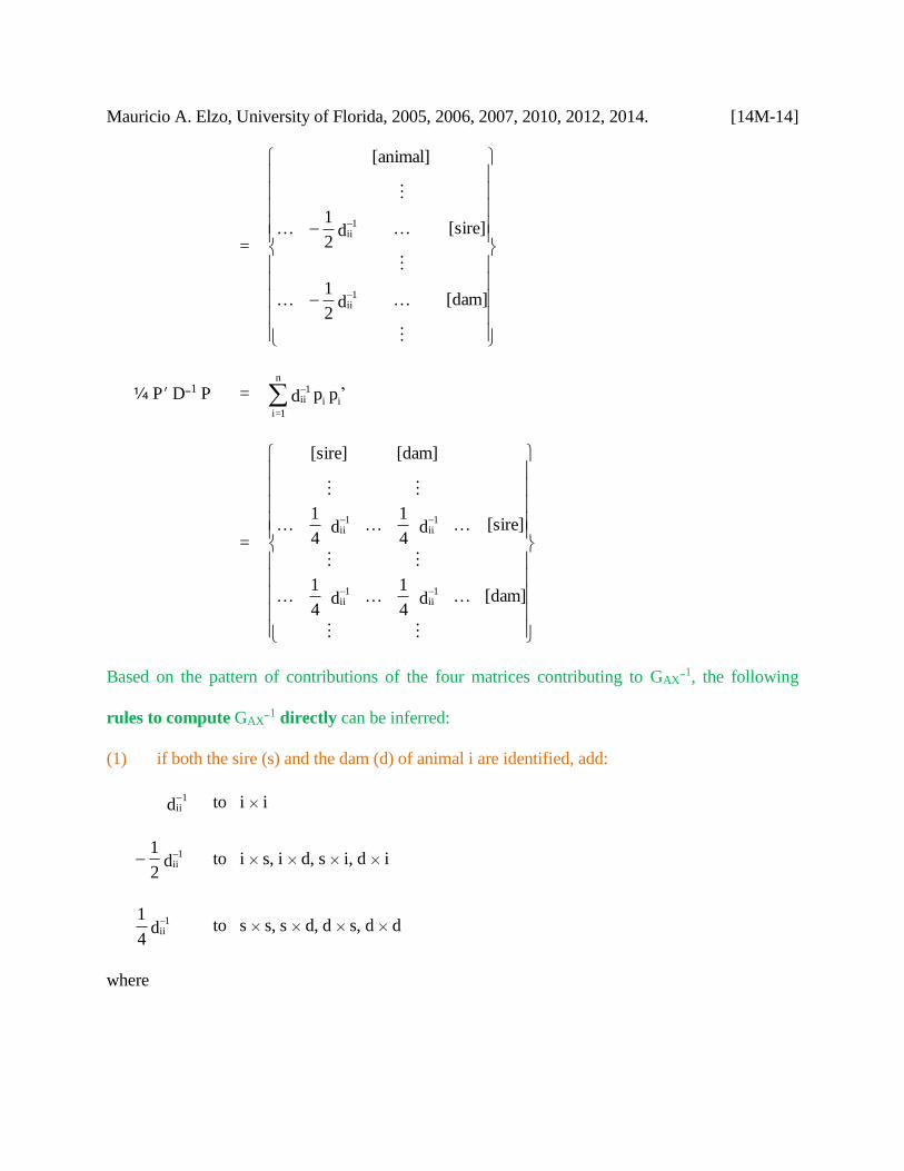
Mauricio A. Elzo, University of Florida, 2005, 2006, 2007, 2010, 2012, 2014. [14M-14]
=
[dam]d 2
1
[sire]d 2
1
[animal]
1ii
1ii
3 P DB1 P = ’p p d ii
1ii
n
1=i
=
[dam]d 4
1d
4
1
[sire]d 4
1d
4
1
[dam][sire]
1ii
1ii
1ii
1ii
Based on the pattern of contributions of the four matrices contributing to GAXB1, the following
rules to compute GAXB1 directly can be inferred:
(1) if both the sire (s) and the dam (d) of animal i are identified, add:
d 1
ii to i i
d 2
1 1ii to i s, i d, s i, d i
d 4
1 1ii to s s, s d, d s, d d
where
Mauricio A. Elzo, University of Florida, 2005, 2006, 2007, 2010, 2012, 2014. [14M-15]
1
iid 1
cd
2
AX
n
1c
cdd
2
AX41
cs
2
AX
n
1c
css
2
AX41
i
2
AX
cdcs
FF
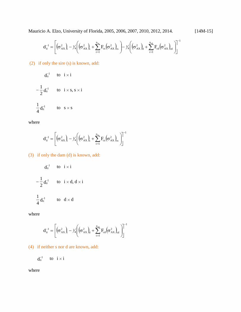
(2) if only the sire (s) is known, add:
d 1
ii to i i
d 2
1 1ii to i s, s i
d 4
1 1ii to s s
where
1
iid 1
cs
2
AX
n
1c
css
2
AX41
i
2
AX
cs
F
(3) if only the dam (d) is known, add:
d 1
ii to i i
d 2
1 1ii to i d, d i
d 4
1 1ii to d d
where
1
iid 1
cd
2
AX
n
1c
cdd
2
AX41
i
2
AX
cd
F
(4) if neither s nor d are known, add:
d 1
ii to i i
where
Mauricio A. Elzo, University of Florida, 2005, 2006, 2007, 2010, 2012, 2014. [14M-16]
d 1
ii = 1
i
2
AX
These computational rules correspond to the multibreed version of Henderson's rules.
In order to apply these rules we must know the dii. If there is no inbreeding the dii can be easily
computed using only the multibreed additive genetic covariances of the genetic groups of the
animal, its sire, and its dam. But, if there is inbreeding, the computation of the dii requires
knowledge of the inbreeding coefficients of each common ancestor of an animal and its
corresponding multibreed variance for trait X. Because we are computing GAX-1 without computing
GAX first, it is easier to compute the dii directly using a recursive procedure based on computing C,
where CC = GAX. This approach will be used here.
Rules to compute the dii in a non-inbred multibreed population
If all animals in a multibreed population are non-inbred then:
(1) if both the sire (s) and the dam (d) of animal i are identified, add:
d 1
ii to i i
d 2
1 1ii to i s, i d, s i, d i
d 4
1 1ii to s s, s d, d s, d d
where
1
iid 1
d
2
AX41
s
2
AX41
i
2
AX
(2) if only the sire (s) is known, add:
d 1
ii to i i
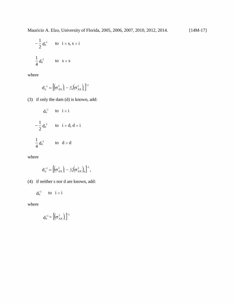
Mauricio A. Elzo, University of Florida, 2005, 2006, 2007, 2010, 2012, 2014. [14M-17]
d 2
1 1ii to i s, s i
d 4
1 1ii to s s
where
1
iid 1
s
2
AX41
i
2
AX
(3) if only the dam (d) is known, add:
d 1
ii to i i
d 2
1 1ii to i d, d i
d 4
1 1ii to d d
where
1
iid 1
d
2
AX41
i
2
AX
,
(4) if neither s nor d are known, add:
d 1
ii to i i
where
d 1
ii = 1
i
2
AX
Mauricio A. Elzo, University of Florida, 2005, 2006, 2007, 2010, 2012, 2014. [14M-18]
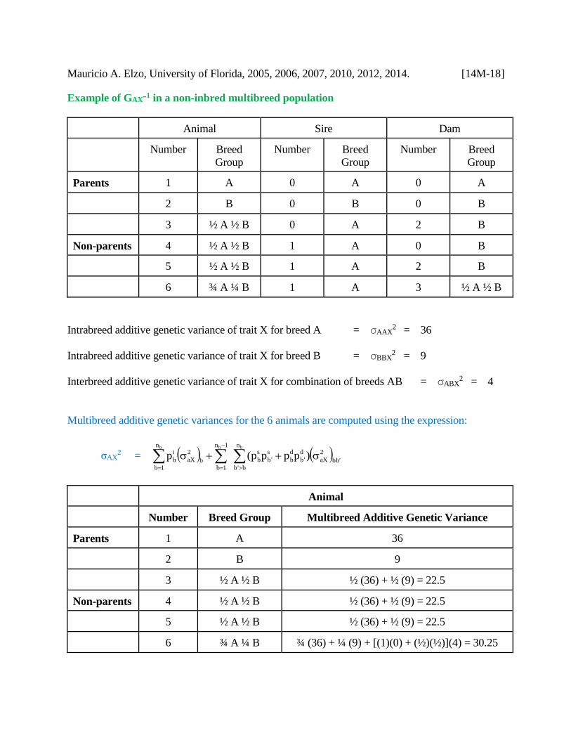
Example of GAXB1 in a non-inbred multibreed population
Animal Sire Dam
Number Breed
Group
Number Breed
Group
Number Breed
Group
Parents 1 A 0 A 0 A
2 B 0 B 0 B
3 ½ A ½ B 0 A 2 B
Non-parents 4 ½ A ½ B 1 A 0 B
5 ½ A ½ B 1 A 2 B
6 ¾ A ¼ B 1 A 3 ½ A ½ B
Intrabreed additive genetic variance of trait X for breed A = AAX2 = 36
Intrabreed additive genetic variance of trait X for breed B = BBX2 = 9
Interbreed additive genetic variance of trait X for combination of breeds AB = ABX2 = 4
Multibreed additive genetic variances for the 6 animals are computed using the expression:
σAX2 =
'bb
2
aX
n
b'b
d
'b
d
b
s
'b
s
b
n
1b
1n
1bb
2
aX
i
b
bb b
)pppp(p
Animal
Number Breed Group Multibreed Additive Genetic Variance
Parents 1 A 36
2 B 9
3 ½ A ½ B ½ (36) + ½ (9) = 22.5
Non-parents 4 ½ A ½ B ½ (36) + ½ (9) = 22.5
5 ½ A ½ B ½ (36) + ½ (9) = 22.5
6 ¾ A ¼ B ¾ (36) + ¼ (9) + [(1)(0) + (½)(½)](4) = 30.25
Mauricio A. Elzo, University of Florida, 2005, 2006, 2007, 2010, 2012, 2014. [14M-19]
The (dii)-1 values for the 6 animals are:
Animal
Number Breed Group (dii)-1
Parents 1 A (36)-1
2 B (9)-1
3 ½ A ½ B 22.5 – ¼ (9) = (20.25)-1
Non-parents 4 ½ A ½ B 22.5 – ¼ (36) = (13.5)-1
5 ½ A ½ B 22.5 – ¼ (36) – ¼ (9) = (11.25)-1
6 ¾ A ¼ B 30.25 – ¼ (36) – ¼ (22.5) = (15.625)-1
The inverse of the GAX matrix is: GAXB1 = DB1 B 2 DB1 P B 2 P DB1 + 3 P DB1 P, where :
P =
000|101
00|011
0|001
---|---
|010
| 00
| 0
,
DB1 =
1
1
1
1
1
1
)15.625(|
)25.11(|
)5.13(|
|
|)25.20(
|)9(
|)36(
, thus
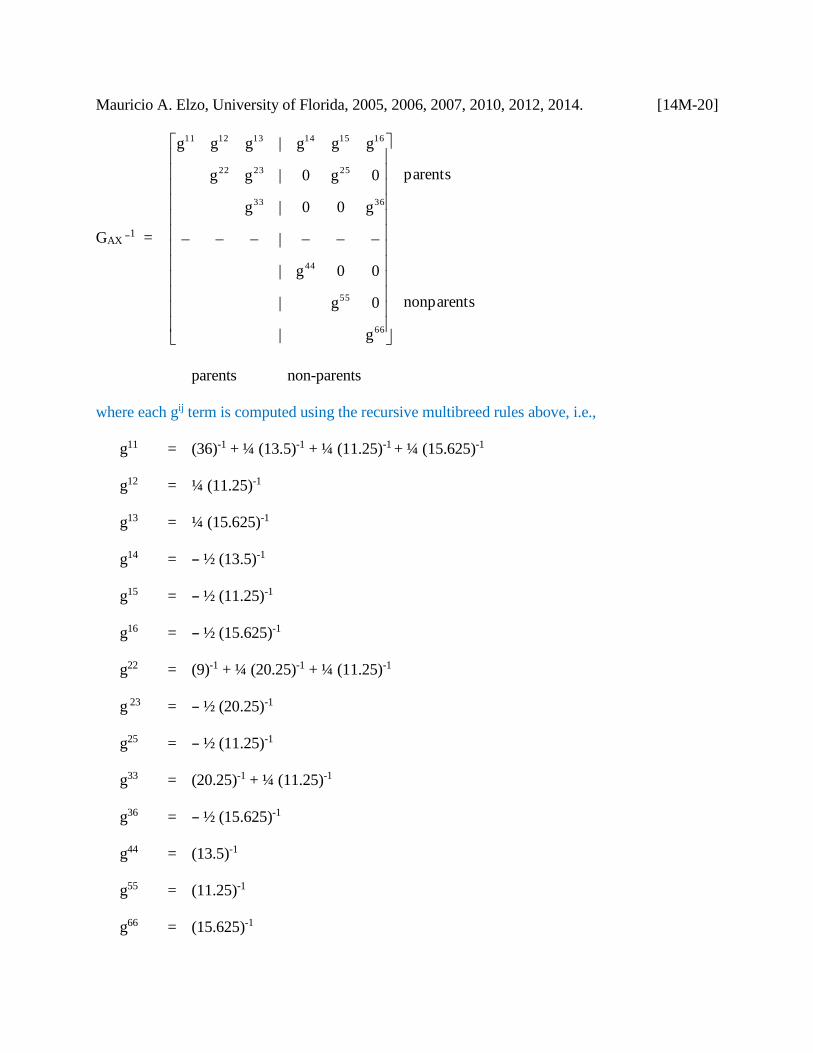
Mauricio A. Elzo, University of Florida, 2005, 2006, 2007, 2010, 2012, 2014. [14M-20]
GAX B1 =
nonparents
parents
g|
0g|
00g|
|
g00|g
0g0|gg
ggg|ggg
66
55
44
3633
252322
161514131211
parents non-parents
where each gij term is computed using the recursive multibreed rules above, i.e.,
g11 = (36)-1 + ¼ (13.5)-1 + ¼ (11.25)-1 + ¼ (15.625)-1
g12 = ¼ (11.25)-1
g13 = ¼ (15.625)-1
g14 = B ½ (13.5)-1
g15 = B ½ (11.25)-1
g16 = B ½ (15.625)-1
g22 = (9)-1 + ¼ (20.25)-1 + ¼ (11.25)-1
g 23 = B ½ (20.25)-1
g25 = B ½ (11.25)-1
g33 = (20.25)-1 + ¼ (11.25)-1
g36 = B ½ (15.625)-1
g44 = (13.5)-1
g55 = (11.25)-1
g66 = (15.625)-1
Mauricio A. Elzo, University of Florida, 2005, 2006, 2007, 2010, 2012, 2014. [14M-21]
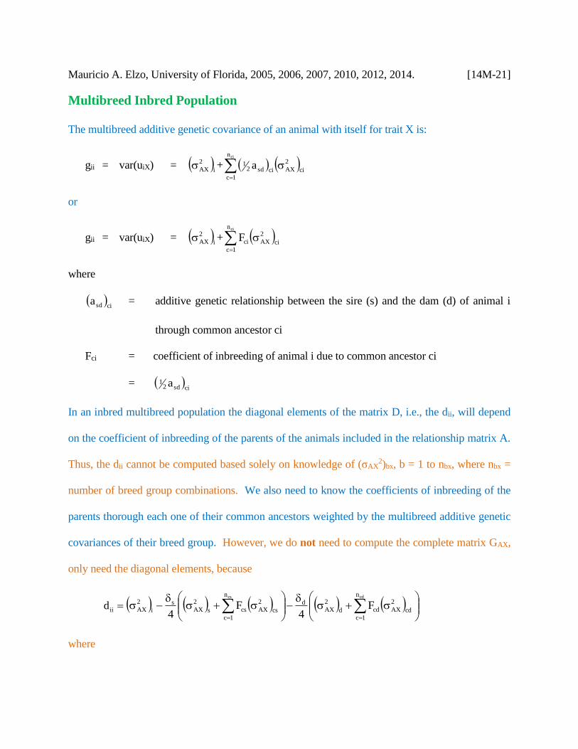
Multibreed Inbred Population
The multibreed additive genetic covariance of an animal with itself for trait X is:
gii = var(uiX) = i
2
AX + ci
2
AX
n
1ccisd2
1
ci
a
or
gii = var(uiX) = i
2
AX + ci
2
AX
n
1c
ci
ci
F
where
cisda = additive genetic relationship between the sire (s) and the dam (d) of animal i
through common ancestor ci
Fci = coefficient of inbreeding of animal i due to common ancestor ci
= cisd2
1 a
In an inbred multibreed population the diagonal elements of the matrix D, i.e., the dii, will depend
on the coefficient of inbreeding of the parents of the animals included in the relationship matrix A.
Thus, the dii cannot be computed based solely on knowledge of (σAX2)bx, b = 1 to nbx, where nbx =
number of breed group combinations. We also need to know the coefficients of inbreeding of the
parents thorough each one of their common ancestors weighted by the multibreed additive genetic
covariances of their breed group. However, we do not need to compute the complete matrix GAX,
only need the diagonal elements, because
iid
cd
2
AX
n
1c
cdd
2
AXd
cs
2
AX
n
1c
css
2
AXs
i
2
AX
cdcs
F4
F4
where
Mauricio A. Elzo, University of Florida, 2005, 2006, 2007, 2010, 2012, 2014. [14M-22]
otherwise0
known is d s if1 ds
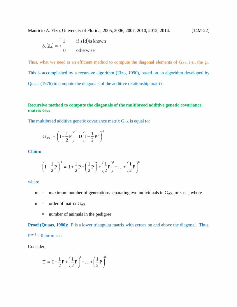
Thus, what we need is an efficient method to compute the diagonal elements of GAX, i.e., the gii.
This is accomplished by a recursive algorithm (Elzo, 1990), based on an algorithm developed by
Quaas (1976) to compute the diagonals of the additive relationship matrix.
Recursive method to compute the diagonals of the multibreed additive genetic covariance
matrix GAX
The multibreed additive genetic covariance matrix GAX is equal to:
’ P2
1I D P
2
1I G
11
AX
Claim:
P2
1 + + P
2
1 + P
2
1 + P
2
1 + I P
2
1I
m321
where
m = maximum number of generations separating two individuals in GAX, m n , where
n = order of matrix GAX
= number of animals in the pedigree
Proof (Quaas, 1986): P is a lower triangular matrix with zeroes on and above the diagonal. Thus,
Pm+1 = 0 for m n.
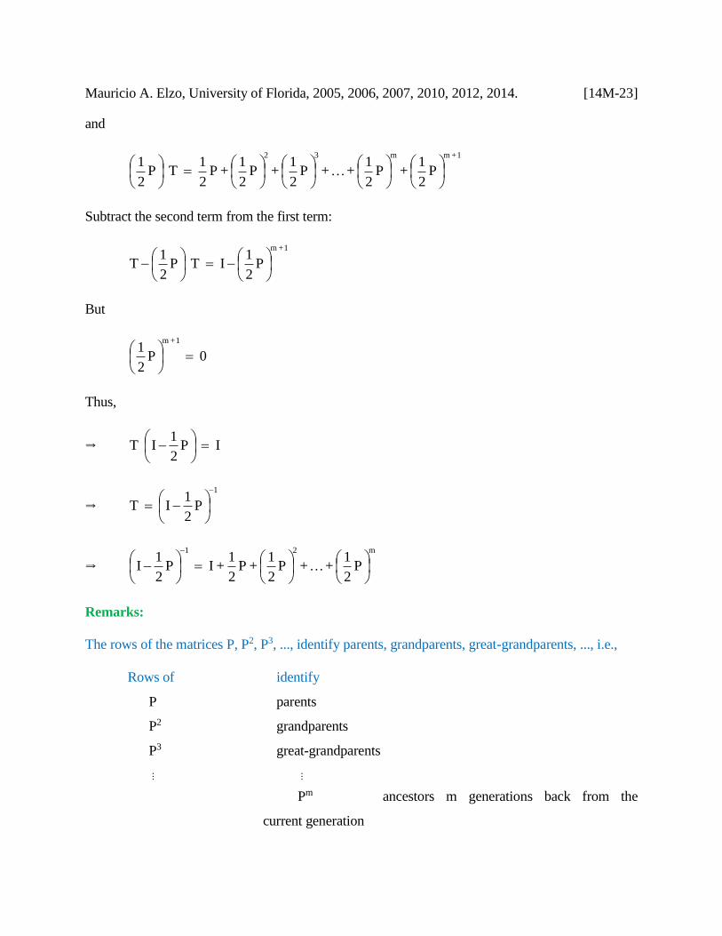
Consider,
P
2
1 + + P
2
1 + P
2
1 + I T
m2
Mauricio A. Elzo, University of Florida, 2005, 2006, 2007, 2010, 2012, 2014. [14M-23]
and
P
2
1 + P
2
1 + + P
2
1 + P
2
1 + P
2
1 T P
2
11 + mm32
Subtract the second term from the first term:
P
2
1I T P
2
1 T
1 + m
But
0 P2
11 + m
Thus,
I P2
1I T
P2
1I T
1
P2
1 + + P
2
1 + P
2
1 + I P
2
1I
m21
Remarks:
The rows of the matrices P, P2, P3, ..., identify parents, grandparents, great-grandparents, ..., i.e.,
Rows of identify
P parents
P2 grandparents
P3 great-grandparents
Pm ancestors m generations back from the
current generation
Mauricio A. Elzo, University of Florida, 2005, 2006, 2007, 2010, 2012, 2014. [14M-24]
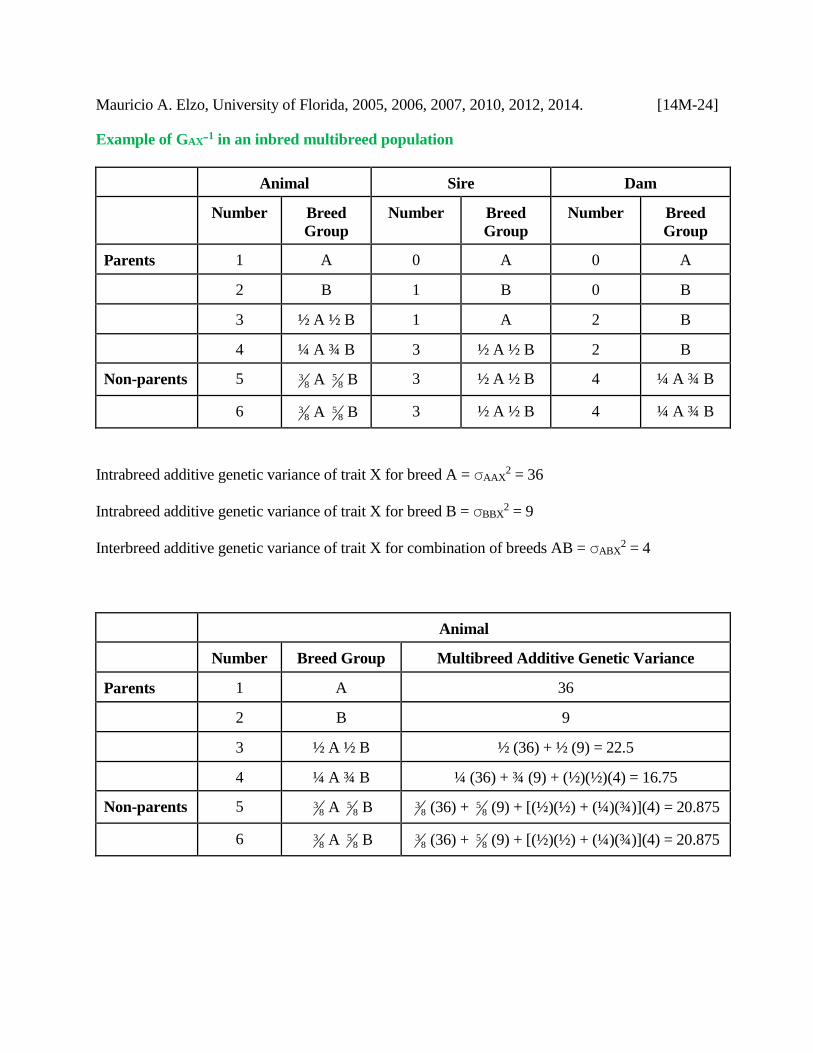
Example of GAXB1 in an inbred multibreed population
Animal Sire Dam
Number Breed
Group
Number Breed
Group
Number Breed
Group
Parents 1 A 0 A 0 A
2 B 1 B 0 B
3 ½ A ½ B 1 A 2 B
4 ¼ A ¾ B 3 ½ A ½ B 2 B
Non-parents 5 83 A 8
5 B 3 ½ A ½ B 4 ¼ A ¾ B
6 83 A 8
5 B 3 ½ A ½ B 4 ¼ A ¾ B
Intrabreed additive genetic variance of trait X for breed A = AAX2 = 36
Intrabreed additive genetic variance of trait X for breed B = BBX2 = 9
Interbreed additive genetic variance of trait X for combination of breeds AB = ABX2 = 4
Animal
Number Breed Group Multibreed Additive Genetic Variance
Parents 1 A 36
2 B 9
3 ½ A ½ B ½ (36) + ½ (9) = 22.5
4 ¼ A ¾ B ¼ (36) + ¾ (9) + (½)(½)(4) = 16.75
Non-parents 5 83 A 8
5 B 83 (36) + 8
5 (9) + [(½)(½) + (¼)(¾)](4) = 20.875
6 83 A 8
5 B 83 (36) + 8
5 (9) + [(½)(½) + (¼)(¾)](4) = 20.875
Mauricio A. Elzo, University of Florida, 2005, 2006, 2007, 2010, 2012, 2014. [14M-25]
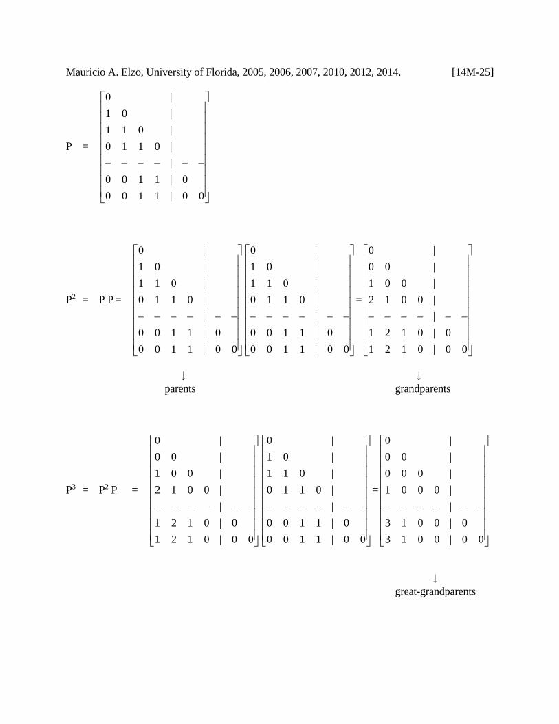
P =
00|1100
0|1100
|
|0110
|011
|01
|0
P2 = P P =
00|1100
0|1100
|
|0110
|011
|01
|0
00|1100
0|1100
|
|0110
|011
|01
|0
=
00|0121
0|0121
|
|0012
|001
|00
|0
parents grandparents
P3 = P2 P =
00|0121
0|0121
|
|0012
|001
|00
|0
00|1100
0|1100
|
|0110
|011
|01
|0
=
00|0013
0|0013
|
|0001
|000
|00
|0
great-grandparents
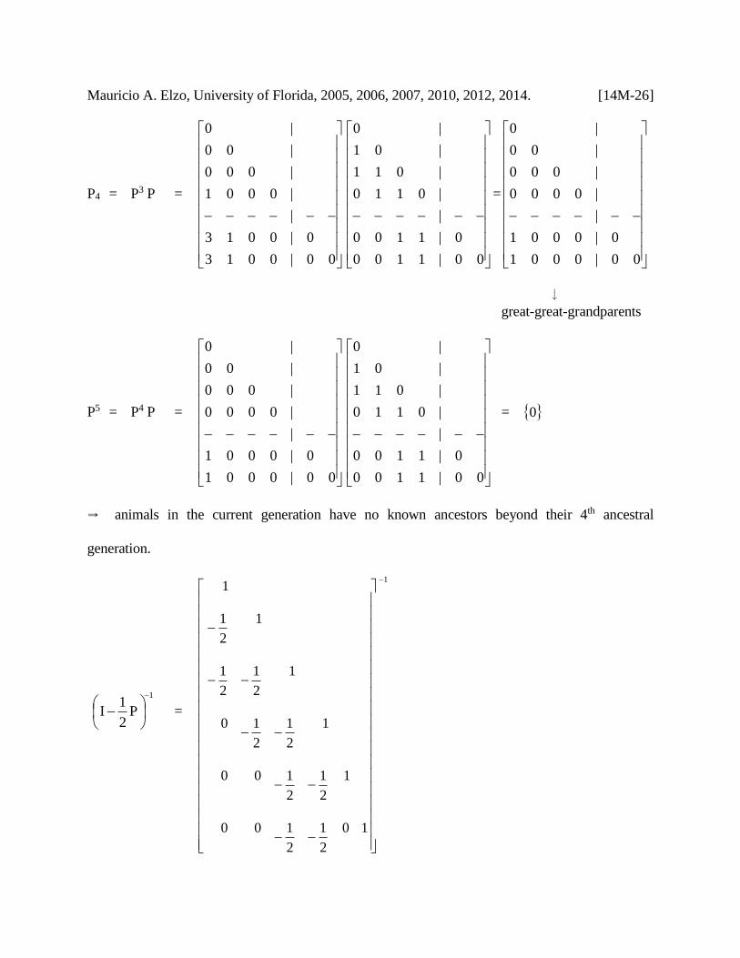
Mauricio A. Elzo, University of Florida, 2005, 2006, 2007, 2010, 2012, 2014. [14M-26]
P4 = P3 P =
00|0013
0|0013
|
|0001
|000
|00
|0
00|1100
0|1100
|
|0110
|011
|01
|0
=
00|0001
0|0001
|
|0000
|000
|00
|0
great-great-grandparents
P5 = P4 P =
00|0001
0|0001
|
|0000
|000
|00
|0
00|1100
0|1100
|
|0110
|011
|01
|0
= 0
animals in the current generation have no known ancestors beyond their 4th ancestral
generation.
P2
1I
1
=
10
2
1
2
100
1
2
1
2
100
1
2
1
2
10
1
2
1
2
1
1
2
1
1 1
Mauricio A. Elzo, University of Florida, 2005, 2006, 2007, 2010, 2012, 2014. [14M-27]
P2
1I
1
=
1.0 0 0.5 0.750.6250.6875
1.0 0.5 0.750.6250.6875
1.0 0.5 0.75 0.625
1.0 0.5 0.75
1.0 0.5
1.0
Alternatively,
P2
1I
1
=
P
2
1 + P
2
1 + P
2
1 + P
2
1 + I
432
=
005.05.000
05.05.000
05.05.00
05.05.0
05.0
0
1
1
1
1
1
1
+
0000125.0375.0
000125.0375.0
000125.0
000
00
0
10025.050.025.0
1025.050.025.0
0025.050.0
0025.0
00
0
+
000000625.0
00000625.0
0000
000
00
0
Mauricio A. Elzo, University of Florida, 2005, 2006, 2007, 2010, 2012, 2014. [14M-28]
P2
1I
1
=
10 0.5 0.750.6250.6875
1 0.5 0.750.6250.6875
1 0.5 0.75 0.625
1 0.5 0.75
1 0.5
1
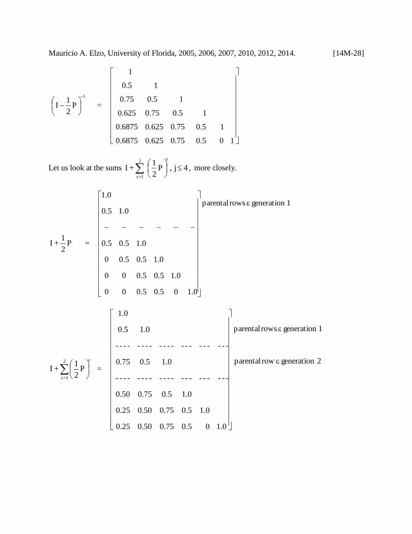
Let us look at the sums , 4 j , P2
1 + I
cj
1=c
more closely.
P2
1 + I =
1 generation rows parental
0.105.05.000
0.15.05.000
0.15.05.00
0.15.05.0
0.15.0
0.1
P
2
1 + I
c2
1=c
= 2 generation row parental
1 generation rows parental
1.000.50.750.500.25
1.00.50.750.500.25
1.0 0.50.750.50
---------------------
1.0 0.50.75
---------------------
1.0 0.5
1.0

Mauricio A. Elzo, University of Florida, 2005, 2006, 2007, 2010, 2012, 2014. [14M-29]
P
2
1 + I
c3
1=c
=
3 generation row parental
2 generation row parental
1 generation rows parental
1.000.50.750.6250.625
1.00.50.750.6250.625
------------------------
1.0 0.5 0.750.625
---------------------
1.0 0.5 0.75
---------------------
1.0 0.5
1.0
P
2
1 + I
c4
1=c
=
3 generation row parental
2 generation row parental
1 generation rows parental
1.000.50.750.6250.6875
1.00.50.750.6250.6875
-------------------------
1.0 0.5 0.75 0.625
------------------------
1.0 0.5 0.75
------------------------
1.0 0.5
1.0
Generalizing:
(1) The ith row of T =
P2
1I
1
is equal to the sum of the ith rows of I, P2
1,
P
2
12
, ...,
P
2
1m
, i.e., ith row of T is equal to the sum of the ith rows of I, P2
1,
P
2
12
, ...,
P
2
1m
.
Mauricio A. Elzo, University of Florida, 2005, 2006, 2007, 2010, 2012, 2014. [14M-30]
However, the ith row of T is also equal to the sum of the ith rows of I, P2
1,
P
2
12
, ...,
P
2
1mi
, where mi (mi ≤ m) is the number of generations separating animal i from its oldest
known ancestor.
(2) The parental rows of P2
1 I are the same as the corresponding ones of
, ,P2
1 + P
2
1 + P
2
1 + I , P
2
1 + P
2
1 + I
322
and of
T P2
1 + + P
2
1 + P
2
1 + P
2
1 + I
m32
.
Similarly, the parental rows of
P
2
1 + P
2
1 + I
2
are the same as the corresponding ones of
P
2
1 + P
2
1 + P
2
1 + I
32
, ..., and T; etc. The reason for it is that the differences that exist between
P
2
1 + I
c1_j
1=c
and
P
2
1 + I
cj
1=c
are related to accounting for the passage of alleles, from ancestors c generations removed form
each animal, to these same individuals. For instance, if c = 3, the difference between
P
2
1 + I
c2
1=c
and
P
2
1 + I
c3
1=c
, are the elements of
P
2
13
which reflect the passage of alleles from great-
grandparents to great-grandprogeny. Thus, rows of animals with unknown ancestors from the cth
generation backwards remain unchanged, i.e., when the passage of alleles from all known
Mauricio A. Elzo, University of Florida, 2005, 2006, 2007, 2010, 2012, 2014. [14M-31]
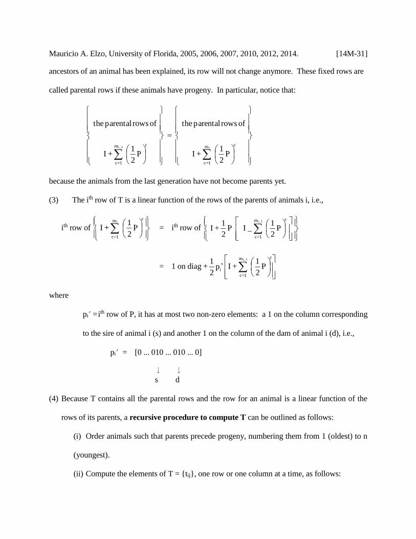
ancestors of an animal has been explained, its row will not change anymore. These fixed rows are
called parental rows if these animals have progeny. In particular, notice that:
P
2
1 + I
of rows parental the
P2
1 + I
of rows parental the
cm
1=c
cm
1=c
i1_i
because the animals from the last generation have not become parents yet.
(3) The ith row of T is a linear function of the rows of the parents of animals i, i.e.,
ith row of
P
2
1 + I
cm
1=c
i
= ith row of
P
2
1 _ I P
2
1 + I
cm
1=c
1_i
= 1 on diag +
P
2
1 + I ’p
2
1cm
1=c
i
1_i
where
pi = ith row of P, it has at most two non-zero elements: a 1 on the column corresponding
to the sire of animal i (s) and another 1 on the column of the dam of animal i (d), i.e.,
pi = [0 ... 010 ... 010 ... 0]
s d
(4) Because T contains all the parental rows and the row for an animal is a linear function of the
rows of its parents, a recursive procedure to compute T can be outlined as follows:
(i) Order animals such that parents precede progeny, numbering them from 1 (oldest) to n
(youngest).
(ii) Compute the elements of T = {tij}, one row or one column at a time, as follows:
Mauricio A. Elzo, University of Florida, 2005, 2006, 2007, 2010, 2012, 2014. [14M-32]
(a) tij = i < jfor t2
1 + t
2
1j , dj , s ii
if si and di are known,
= i < jfor t2
1j , si
if si is known only,
= i < jfor t2
1j , di
if di is known only,
= i < jfor 0 if neither si nor di is known,
= i > jfor 0
(b) tii = 1
The matrix GAX, written in terms of T, is:
GAX = T D T
Because D is diagonal and positive, D = D2 D2. Thus,
GAX = T D2 D2 T
GAX = CC
where
C = T D2
C = Cholesky decomposition of GAX
The elements of C can be computed recursively, using the procedure to compute T, as follows:
(i) cij = d t 21
jjij
= i < jfor d t + t 2
12
1
iiii jjj , ddj , ss
where
ds ii = 1 if si (di) > 0
Mauricio A. Elzo, University of Florida, 2005, 2006, 2007, 2010, 2012, 2014. [14M-33]
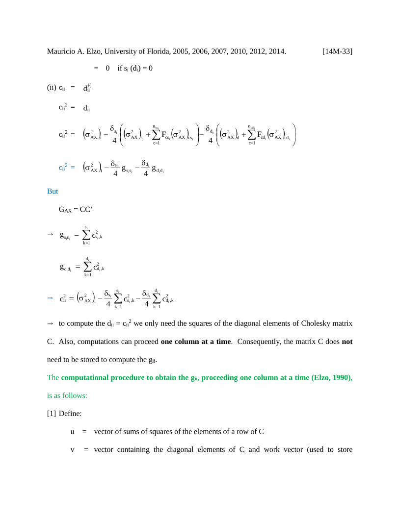
= 0 if si (di) = 0
(ii) cii = d 21
ii
cii2 = dii
cii2 =
i
icd
i
i
i
ics
ii
i
cd
2
AX
n
1c
cdd
2
AX
d
cs
2
AX
n
1c
css
2
AX
s
i
2
AX F4
F4
cii2 =
ii
i
ii dd
d
ssis
i
2
AX g 4
g 4
But
GAX = CC
c g 2k,s
s
1=k
ss i
i
ii
c g 2k,d
d
1=k
dd i
i
ii
c 4
c 4
c2
k,d
d
1=k
d2k,s
s
1=k
s
i
2
AX2ii i
i
i
i
i
i
to compute the dii = cii2 we only need the squares of the diagonal elements of Cholesky matrix
C. Also, computations can proceed one column at a time. Consequently, the matrix C does not
need to be stored to compute the gii.
The computational procedure to obtain the gii, proceeding one column at a time (Elzo, 1990),
is as follows:
[1] Define:
u = vector of sums of squares of the elements of a row of C
v = vector containing the diagonal elements of C and work vector (used to store
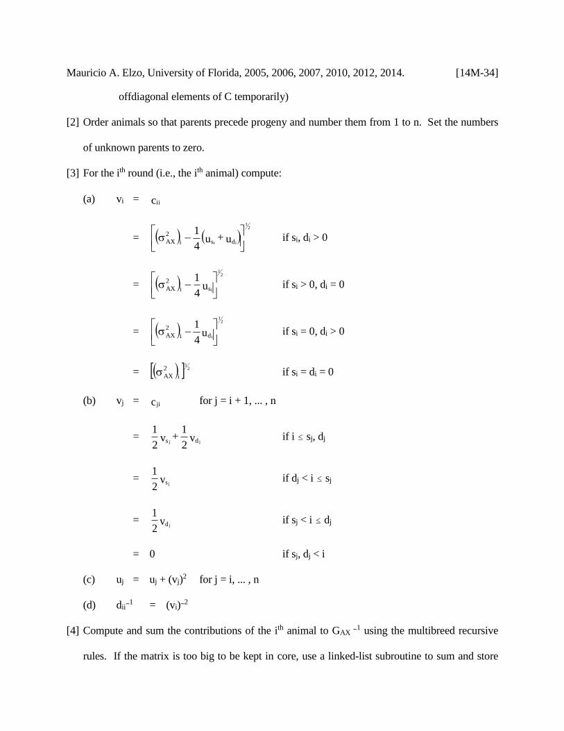
Mauricio A. Elzo, University of Florida, 2005, 2006, 2007, 2010, 2012, 2014. [14M-34]
offdiagonal elements of C temporarily)
[2] Order animals so that parents precede progeny and number them from 1 to n. Set the numbers
of unknown parents to zero.
[3] For the ith round (i.e., the ith animal) compute:
(a) vi = cii
=
u + u
4
1 dsi
2
AX ii
21
if si, di > 0
=
u
4
1 si
2
AX i
21
if si > 0, di = 0
=
u
4
1 di
2
AX i
21
if si = 0, di > 0
= 21
i
2
AX if si = di = 0
(b) vj = c ji for j = i + 1, ... , n
= v2
1 + v
2
1ds jj
if i sj, dj
= v2
1s j
if dj < i sj
= v2
1d j
if sj < i dj
= 0 if sj, dj < i
(c) uj = uj + (vj)2 for j = i, ... , n
(d) diiB1 = (vi)B
2
[4] Compute and sum the contributions of the ith animal to GAX B1 using the multibreed recursive
rules. If the matrix is too big to be kept in core, use a linked-list subroutine to sum and store
Mauricio A. Elzo, University of Florida, 2005, 2006, 2007, 2010, 2012, 2014. [14M-35]
only the non-zero elements of GAXB1.
[5] Repeat steps [3] and [4] until the last animal is processed, i.e., do steps [3] and [4] for i = 1, ... ,
n.
[6] If matrix GAXB1 is to be stored on disk or type, copy the non-zero elements accompanied by
their row and column numbers.
References
Falconer, D. S. 1981. Introduction to Quantitative Genetics. 2nd Ed., Longman, Inc., New York.
Henderson, C. R. 1976. A simple method for computing the inverse of a large numerator
relationship matrix used in prediction of breeding values. Biometrics 32:69-83.
Elzo, M. A. 1990. Recursive procedures to compute the inverse of the multiple trait additive
genetic covariance matrix in inbred and noninbred multibreed populations. J. Anim. Sci.
68:1215-1228.
Elzo, M. A. 1996. Animal Breeding Notes. University of Florida, Gainesville, Florida, USA.
Quaas, R. L. 1975. From Mendel's laws to the A inverse. Mimeograph, Cornell University, p 16.
Quaas, R. L. 1976. Computing the diagonal elements and inverse of a large numerator relationship
matrix. Biometrics 32:949-953.
Quaas, R. L. 1986. Personal Communication. Animal Science 720. Cornell University, Ithaca,
NY.
![ANIMAL BREEDING NOTES - animal.ifas.ufl.edu fileMauricio A. Elzo, University of Florida, 2005, 2006, 2007, 2010, 2014. [16M - 1] ANIMAL BREEDING NOTES CHAPTER 16M EQVE EQVA MULTIBREED](https://img.pdfslide.us/doc/110x75/5e1040a6d4c3cc2b166fecc9/animal-breeding-notes-a-elzo-university-of-florida-2005-2006-2007-2010.jpg)