The Jolly-Seber model: more than just

abundance

Carl J. Schwarz�

Abstract

The Jolly-Seber model provides estimates of abundance, survival,

and capture rates from capture-recapture experiments. We will re-

view the use of the Jolly-Seber model in open populations for these

purposes and the recent extensions of the single cohort model to the

following cases: (a) multiple-cohort studies where recruitment rates

are compared among cohorts; (b) age-speci�c breeding proportions;

(c) population growth rates. Finally, we propose new areas of research

needed for this model.

�Carl J. Schwarz is an Associate Professor, Department of Mathematics and Statistics,

Simon Fraser University, Burnaby, BC V5A 1S6, Canada (e-mail: cschwarz@cs.sfu.ca).

1

Keywords: animal abundance; breeding proportions; capture-recapture;

Cormack-Jolly-Seber; Jolly-Seber; mark-recapture; survival estima-

tion;

2

1 Introduction

It is now just over 40 years since Darroch (1959) developed models for open-

population capture-recapture experiments. This was only a partial solution

as his paper derived both estimators and variances only for populations with

either immigration or death (but not both) and derived moment estimators

only for populations with both sources of change. It was not until six years

later that both Jolly (1965) and Seber (1965) in back-to-back papers derived

both estimators and variances for the general case.

Since that time, extensive work has been done on capture-recapture mod-

els with Seber (1982), Seber (1986), Seber (1992) and Schwarz and Seber

(1999) providing extensive reviews. Work in this �eld can be broadly di-

vided into three areas: closed population models; death only models fol-

lowing marked animals over time { the Cormack-Jolly-Seber (CJS) models

(Cormack, 1964; Jolly, 1965; Seber, 1965); and birth and death models { the

Jolly-Seber (JS) model (Jolly, 1965; Seber, 1965).

Development of methods for closed populations has been extensive. Mod-

els have been developed accounting for various sources of heterogeneity in

3

catchability (the M0;Mt;Mh; : : : suite); di�erent ways of handling hetero-

geneity (sample coverage methods of Chao, Lee, and Jeng (1992); the non-

parametric MLE method (Norris and Pollock, 1996)); and di�erent ways of

�tting models (log-linear methods of Cormack (1989, 1993); maximum likeli-

hood; Horvitz-Thompson method of Huggins (1989); martingale methods of

Lloyd and Yip (1991). Powerful software is available (CAPTURE by White

et al. 1982).

Many developments of models for the Cormack-Jolly-Seber approach have

also occurred. Lebreton et al. (1992) extended the method to multiple groups

in an ANOVA-type framework. Schwarz, Schweigert, and Arnason (1993),

and Brownie et at. (1993) introduced movement models. Burnham (1993)

and Barker (1997) showed how to combine both recapture resightings, and

returns of dead animals. Powerful software (MARK by White and Burnham,

1999; SURGE by Pradel and Lebreton, 1991) have been developed to assist

in model �tting and selection. In all of these approaches, emphasis has

been placed on modelling survival rates. Because only marked animals were

followed over time, no estimates of abundance are available.

Surprisingly, much less work has been done on Jolly-Seber models where

4

abundance estimation is also possible. Part of the reason is related to ex-

perimental design issues. The experimental protocol needed to successfully

follow only marked animals over time is much less rigorous than that needed

to also model the introduction of new unmarked animals into the population.

Another reason is that raw abundance estimates are not that interesting to

ecologists - rather trends in abundance or relative abundance may be of

more interest. In recent years, there have been a resurgence of interest in the

Jolly-Seber model focusing on more than simple abundance.

This paper will review and summarize three recent developments in the

JS model that more the emphasis away from simply abundance estimation.

These are:

� modelling the pattern of entrance of new recruits. This required the

development of a new likelihood formulation.

� modelling age-speci�c breeding proportions. Clobert et al. (1994) used

the CJS framework for this, but a more natural framework is a modi-

�cation of the JS model.

� modelling population growth, dilution or fecundity. Pradel (1996) and

5

Pradel et al. (1997) used the CJS framework on reversed capture-

histories, but again these quantities fall naturally out of the JS model.

Finally, I speculate on where future research work on the Jolly-Seber

model is needed.

2 Notation

The notation for JS models has been relatively standardized and follows to

a great extent that of the CJS model. Sample occasion are usually denoted

by the subscript i while group membership is denoted by the subscript g.

\Births" refers to any mechanism by which new animals are added at un-

known times to the catchable population (by immigration, recruitment, etc.).

Similarly, \death" refers to all processes that permanently remove animals

from the catchable population (emigration, death, inactivity, etc.). We do

not distinguish between sources of new animals or between the ways animals

leave the population. Births at known sample times (e.g. by deliberate ad-

dition of marked animals) are called injections and deaths at known sample

times are called losses on capture.

6

The notation has been divided into three sections; that for statistics en-

countered in capture-recapture experiment; that for the parameters directly

of interest; and that for functions of the parameters that are also of interest,

or functions useful in writing the likelihood function in a compact form.

Statistics:

mgi number of animals from group g captured at sample time i that were

previously marked.

ugi number of animals from group g captured at sample time i that are

unmarked.

ngi number of animals from group g captured at sample time i. ngi = mgi+

ugi.

Rgi number of animals from group g that are released after the ith sample.

Rgi need not equal ngi if losses on capture or injections of new animals

occur at sample time i.

rgi number of Rgi animals released at sample time i that are recaptured at

one or more future sample times.

zgi number of animals from group g captured before time i, not captured at

time i, and captured after time i.

7

Fundamental Parameters:

k number of sample times.

pgi probability of capture for animals in group g at sample time i

�gi probability of an animal from group g surviving and remaining in the

population between sample time i and sample time i+ 1 given it was

alive and in the population at sample time i

Ng total number of animals in group g that enter the system and survive

until the next sample time. Ng = Bg0 +Bg1 + : : :+Bg;k�1.

�gi fraction of the total net births that enter the system between sample

times i and i+ 1. These as the entry probabilities. �gi = Bgi=Ng.

8

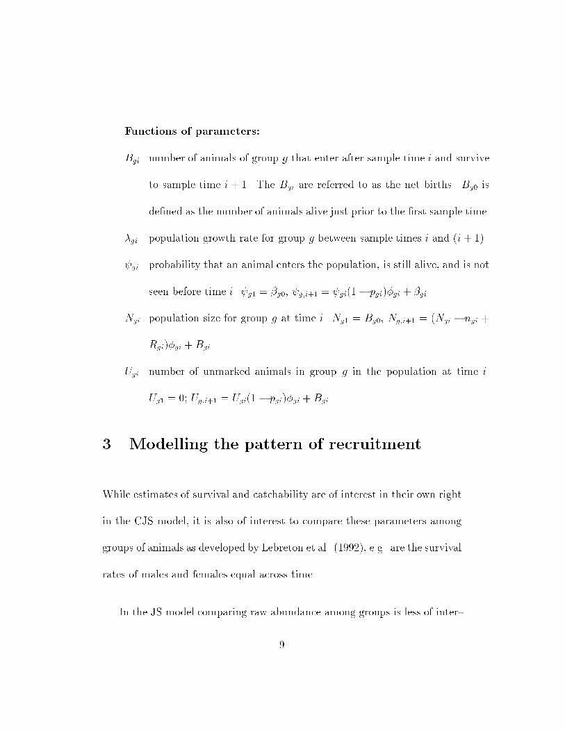
Functions of parameters:

Bgi number of animals of group g that enter after sample time i and survive

to sample time i+ 1. The Bgi are referred to as the net births. Bg0 is

de�ned as the number of animals alive just prior to the �rst sample time.

�gi population growth rate for group g between sample times i and (i+ 1)

gi probability that an animal enters the population, is still alive, and is not

seen before time i. g1 = �g0, g;i+1 = gi(1� pgi)�gi + �gi.

Ngi population size for group g at time i. Ng1 = Bg0, Ng;i+1 = (Ngi � ngi +

Rgi)�gi +Bgi

Ugi number of unmarked animals in group g in the population at time i.

Ug1 = 0; Ug;i+1 = Ugi(1 � pgi)�gi +Bgi

3 Modelling the pattern of recruitment

While estimates of survival and catchability are of interest in their own right

in the CJS model, it is also of interest to compare these parameters among

groups of animals as developed by Lebreton et al. (1992), e.g. are the survival

rates of males and females equal across time.

In the JS model comparing raw abundance among groups is less of inter-

9

est, e.g. is it of ecological interest to compare raw recruitment of di�erent

groups. Rather the relative increase or pattern of increase may be more in-

teresting, e.g. is the pattern of recruitment the same for males and females.

The impediment to a parallel theory of Lebreton et al. (1992) for JS

models was the lack of a suitable parameterization and likelihood function.

Starting with Darroch (1959), it has been well known that the full like-

lihood for a JS capture-recapture experiment can be partitioned into three

components, L = L1 � L2 � L3 = P (�rst capture)� P (losses on capture)�

P (recaptures). The latter two components can be modelled by products

of conditionally independent binomial distributions as shown by Burnham

(1991). It is the �rst component that causes di�culty.

Darroch (1959) derived the likelihood function for the �rst component

in the case of immigration or death (but not both), but was only able to

develop the probability generating function for the more general case. He

treated the Bgi as �xed constants and noted that this likelihood component

involved (k � 1) dimensional sums of probabilities making its maximization

intractable.

10

Six years later, both Jolly (1965) and Seber (1965) independently derived

an explicit expression for this component by assuming that Ugi are �xed

parameters and de�ning Bgi = Ug;i+1 � �gi(Ugi � ugi). The �rst component

can then be explicitly written as a product of binomials:

L1 =GYg=1

kYi=1

0B@Ugi

ugi

1CA (pgi)ugi (1� pgi)

Ugi�ugi

with the simple solution of Ugi = ugi/pgi.

There were several problems with this result. First, `births' do not explic-

itly enter in the likelihood which makes it di�cult to impose constraints upon

the Bgi such as being zero at certain times or being equal among groups at a

particular time, or being a function of covariates. And the likelihood models

the raw counts; translating these to a pattern of recruitment was not feasi-

ble. This makes modelling e�orts along the lines of Lebreton et al. (1992)

extremely di�cult. This formulation also leads to some technical di�culties

such as keeping all the Bgi non-negative and that in the case of no births or

no deaths, the component did not simplify to the likelihoods already derived

for these special cases.

This was the commonly accepted formulation until the mid-90's. Inter-

estingly Cormack (1989) tried a log-linear approach where new recruits were

11

modelled using a population growth rate applied to unmarked animals for-

shadowing Pradel's (1996) paper on population growth. This too su�ered

from some technical problems as outlined in Schwarz and Arnason (1996).

Burnham (1991) also derived an alternate representation but it was not en-

tirely satisfactory.

Over 30 years after Jolly (1965) and Seber (1965), Schwarz and Arnason

(1996) built upon the development of Crosbie and Manly (1985) to develop a

formulation that resolved a number of issues. They treated Bg0; : : : ; Bg;k�1 as

random variables conditional upon Ng (the total number of unique animals in

the experiment in group g), and let �g0; : : : ; �g;k�1 be the fraction of the pop-

ulation that entered between sampling occasions i and i+ 1 and survived to

the next sampling occasion. Hence there are hypothetical super-populations

of Ng animals and Bg0; : : : ; Bg;k�1 � Multinomial (Ng;�g0; : : : ; �g;k�1). This

led to a likelihood for the �rst component of:

L1 =GYg=1

0B@Ng

ug�

1CA kXi=1

gipgi

!ug� 1�

kXi=1

gipgi

!Ng�ug�

�

0B@ ug�

ug1; ug2; : : : ; ugk

1CA kYi=1

0BBB@ gipgikP

i=1

gipgi

1CCCAugi

Here f gig is a function of the relative birth rates f�gig. The likelihood

can now be expressed as a product of multinomial and binomial distributions

12

in much the same way as was done for the CJS model.

The new formulation leads to all the usual estimators of Jolly (1965)

and Seber (1965). Because the parameters describing the `birth' process are

directly available in the likelihood, it is relatively easy to selectively constrain

subsets to be zero, to be equal over time, to be equal among group, or to

be functions of covariates. All the machinery developed for model selection

(likelihood ratio tests and AIC) for the CJS models can be used directly. The

computer package POPAN (Arnason, Schwarz, and Boyer, 1998) implements

all of these modi�cations to the JS models.

Parameterizing in terms of the proportions of new animals that enter

between sampling occasions is also advantageous.

First, it would be quite unusual when conducting an experiment on two

groups of animals whose absolute population sizes could be quite di�erent

to expect that the absolute recruitment would be equal between the two

groups. However, the pattern of recruitment may be equal. Schwarz and

Arnason (1996) presented such an example of salmon returning to spawn

where sampling occurred weekly. Returning salmon can be classi�ed into two

groups: adults who returned at age 3; and jacks which are precocious males

13

returning at age 2. Do the two types of males return in the same pattern?

Extending the notation of Lebreton et al. (1992), Schwarz and Arnason

(1996) used AIC to select the model fpg; �t; �g�tg as the most suitable and the

estimates are shown in Table 1. This shows that adults and jacks had unequal

catchability, had similar survival patterns over time, but more importantly,

the pattern of returns for the two groups was di�erent with jacks tending to

return earlier than adults.

Second, estimates of f�gig are relatively free of the biases caused by het-

erogeneity in catchability - the Achilles heel of raw abundance and raw re-

cruitment estimates. Carothers (1973) showed that the asymptotic relative

bias of Ngi is basically a function of the gi the coe�cient of variation in the

capture-probabilities, i.e. E [Ngi] � Ngi=(1 + 2gi) and that survival estimates

are essentially una�ected. If the coe�cient of variation in catchability is rel-

atively constant over time, then both Bgi � Ng;i+1� Ngi�gi and Ng =k�1Pi=0

Bgi

have the same relative bias, but �gi =Bgi

Ngwill be relatively free of bias. This

has been con�rmed by the author using method similar to Carothers (1973)

and in simulation studies. Hence, it may not be necessary to use methods

such as Pledger and E�ord (1999) to try and correct for heterogeneity in

these cases.

14

Because the f�gig are relatively free of bias caused by heterogeneity in

catchability, it also implies that estimators based on these should also be

relatively una�ected. For example, Manske and Schwarz (in press) devel-

oped an estimator for stream residence of �sh from JS experiments that is

insensitive to heterogeneity in catchability.

4 Age-speci�c breeding proportions

Clobert et al. (1994) used the CJS model to estimate the age-speci�c breeding

probabilities from capture-recapture studies of successive cohorts of animals

marked as young. Prior to age k at which the youngest individual breeds,

animals cannot be observed. Once an animal starts to breed, it may be

recaptured or resighted.

The di�culty in �tting a standard CJS model to this data is that the

marked animals in a cohort after age k but before all animals have become

breeders consists of two subgroups - those who are non-breeders which cannot

be observed and those who are breeders which can be recaptured. This

heterogeneity in the capture probabilities violates a key assumption of the

15

CJS model that all animals alive have the same probability of recapture at a

sampling occasion. Clobert et al. (1994) was forced to introduce a number of

capture-parameters representing the overall, average, probability of capture

during the progression to full breeding status, and it was the changes in these

values that allowed them to estimate the breeding probabilities.

Because it is in changes in the average probabilities of capture that lead to

estimates of the breeding proportions, it is di�cult to numerically constrain

these to be positive, or to test for equality of these parameters among groups,

or to model them as functions of covariates.

However, the age-speci�c breeding proportions can be estimated directly

by �tting a JS model to the capture histories using the initial mark only to

age the animals. Prior parameterizations of the JS model made this di�cult

because the total recruitment between sampling occasions was modelled, and

it was impossible to constrain these to be non-negative or to simultaneously

model several cohorts with common recapture, survival, or recruitment pa-

rameters. The new parameterization avoids many of the nasty model �tting

complications of Clobert et al. (1994) and lends itself to direct model selec-

tion and testing. Furthermore, the Schwarz and Arnason (1996) formulation

16

also naturally leads to multiple-cohort settings.

Let there are G cohorts of animals marked as young (for simplicity at age

0). For convenience we assume that animals start to breed at age 1; that no

further animals start to breed after age m that each capture-occasion is one

year apart ; and that observations on breeders start in calendar year 1 - the

�rst year when the �rst cohort starts to breed. Observations continue until

calendar year T with T � m.

As in Clobert et al. (1994), the following assumptions are made in addi-

tion to those commonly made in CJS models:

� all non-breeders have a 0 probability of recapture;

� all breeding animals, whether for the �rst time or not, have the same

probability of recapture;

� once an animal has bred for the �rst time, it remains a breeder until

the end of the study. [The models could be extended if a maximum

age of breeding was known.]

� all animals, regardless of �rst time or a repeat breeder, have the same

probability of survival in a year. [Note that a more general model

17

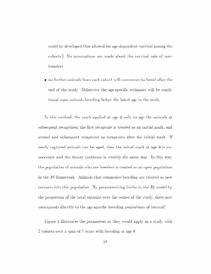
could be developed that allowed for age-dependent survival among the

cohorts.] No assumptions are made about the survival rate of non-

breeders.

� no further animals from each cohort will commence to breed after the

end of the study. Otherwise the age-speci�c estimates will be condi-

tional upon animals breeding before the latest age in the study.

In this method, the mark applied at age 0 only to age the animals at

subsequent recaptures; the �rst recapture is treated as an initial mark, and

second and subsequent recaptures as recaptures after the initial mark. If

newly captured animals can be aged, then the initial mark at age 0 is un-

necessary and the theory continues in exactly the same way. In this way,

the population of animals who are breeders is treated as an open population

in the JS framework. Animals that commence breeding are treated as new

entrants into this population. By parameterizing births in the JS model by

the proportion of the total entrants over the course of the study, these now

corresponds directly to the age-speci�c breeding proportions of interest!

Figure 1 illustrates the parameters as they would apply in a study with

2 cohorts over a span of 7 years with breeding at age 6.

18

The most general model shown in Figure 1 is not very useful as each

cohort has its own set of parameters and there is confounding of parameters

at the start and end of the study as listed in Schwarz et al. (1993). This

implies that the age-speci�c probabilities are not estimable unless further

assumptions are made. For example, the study could be extended at least

one further occasion after the last age of breeding, i.e. ensure that bg;T�i = 0

for all cohorts.

Resolving the confounding at the start of the study can be done by

assuming that certain parameters are equal across cohorts or by model-

ing the capture probabilities as functions of covariates. For example, one

may be willing to assume that the fpgig are cohort-independent, i.e. that

p1i = p2i = � � � = pGi. Or, the fpgig could be modeled as functions of co-

variates (as was done in Clobert et al. 1994) or possibly it may be tenable

to consider models where the pgi are constant over time, i.e., where pgi = pg�

for all i.

Alternatively, it is sometimes possible to have a separate cohort of known

breeders that were marked prior to the start of the �rst recaptures of the new

breeders. In this case, this additional cohort could be used to estimate the

19

p�i (under the assumption of independence of recapture probabilities among

cohorts).

Once the confounding problem has been resolved, the Jolly-Seber model

can be �t using the methods outlined in Schwarz and Arnason (1996) using

the computer package POPAN (Arnason, Schwarz, Boyer 1998) based on the

usual summary statistics.

Reduced models can also be investigated using likelihood ratio tests or

AIC in the usual fashion. An interesting set of models is where the age-

speci�c breeding proportions are stationary over time, i.e. b1i = b2i = � � � =

bGi.

Schwarz and Arnason (in press), and Schwarz and Stobo (in press) present

examples of the application of this model to the black-headed gulls used by

Clobert et al. (1994) and to a population of grey seals that return to breed

on Sable Island, respectively.

The results of the model �tting procedures applied to the gull data are

shown in Table 2. Here all breeding proportion estimates are non-negative

(unlike in Clobert et al. 1994), and it is relatively easy to �t and test if a

20

model with equal breeding proportions over cohorts is tenable.

The average age of �rst breeding is found directly and its standard error

estimated by a Taylor-series expansion.

By making further assumptions about the survival rate of non-breeders,

it was also possible to estimate the juvenile survival rate - however, unless

the cohorts were tagged as young, this would generally not be possible.

The JS method has a number of advantages over that used by Clobert et

al. (1994):

� Estimates of age-speci�c breeding proportions are a fundamental pa-

rameter of the model and are easily estimated using the methodology

of Schwarz and Arnason (1996).

� It is easy to constrain the estimates to be within the admissible range

of 0-1 and to model them as functions of covariates.

� It is straight forward to examinemodels where the breeding proportions

are equal among cohorts.

� The confounding among the breeding proportions, capture probabili-

21

ties, and survival rates at the beginning and end of the study are now

readily apparent and the modeler is aware of the need to estimate some

of the confounded parameters to `free up' the estimates of the breeding

proportions. Suggestions for alleviating this confounding were made

earlier.

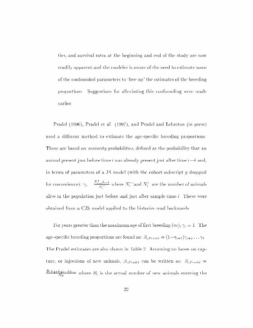
Pradel (1996), Pradel et al. (1997), and Pradel and Lebreton (in press)

used a di�erent method to estimate the age-speci�c breeding proportions.

These are based on seniority probabilities, de�ned as the probability that an

animal present just before time i was already present just after time i�1 and,

in terms of parameters of a JS model (with the cohort subscript g dropped

for convenience): i =N+

i�1�i�1

N�

i

where N�

i and N+i are the number of animals

alive in the population just before and just after sample time i. These were

obtained from a CJS model applied to the histories read backwards.

For years greater than the maximumage of �rst breeding (m), i = 1. The

age-speci�c breeding proportions are found as: �i;P radel = (1� i+1) i+2 : : : T .

The Pradel estimates are also shown in Table 2. Assuming no losses on cap-

ture, or injections of new animals, �i;P radel can be written as: �i;P radel =

Bi�i+1�i+2:::�T�1NT

where Bi is the actual number of new animals entering the

22

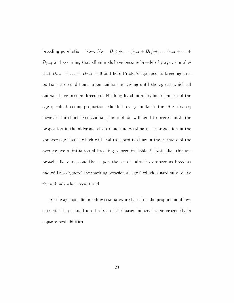
breeding population. Now, NT = B0�1�2 : : : �T�1 + B1�2�3 : : : �T�1 + � � � +

BT�1 and assuming that all animals have become breeders by age m implies

that Bm+1 = : : : = BT�1 = 0 and here Pradel's age speci�c breeding pro-

portions are conditional upon animals surviving until the age at which all

animals have become breeders. For long lived animals, his estimates of the

age-speci�c breeding proportions should be very similar to the JS estimates;

however, for short lived animals, his method will tend to overestimate the

proportion in the older age classes and underestimate the proportion in the

younger age classes which will lead to a positive bias in the estimate of the

average age of initiation of breeding as seen in Table 2. Note that this ap-

proach, like ours, conditions upon the set of animals ever seen as breeders

and will also `ignore' the marking occasion at age 0 which is used only to age

the animals when recaptured.

As the age-speci�c breeding estimates are based on the proportion of new

entrants, they should also be free of the biases induced by heterogeneity in

capture probabilities.

23

5 Population Growth

The JS model was originally developed to estimate raw abundances. How-

ever, in many cases, this is of secondary importance and trend in abundance

(population growth or decline) are of more ecological interest.

Pradel (1996) and Pradel et al. (1997) used the CJS model to capture-

histories read `backwards' to estimate seniority probabilities (and subsequent

fecundity) and population growth. However, as modelling histories in a for-

ward direction leads only to estimates of catchability and survival, modelling

histories in a backwards fashion leads to estimates of catchability and senior-

ity. Consequently, it seems sensible to use a Jolly-Seber model to estimate

all quantities simultaneously.

In the short term, population growth can be expressed in terms of the

Jolly-Seber fundamental parameters (dropping the subscript g for conve-

nience and ignoring losses on captures and injections) as:

�i =N�

i+1

N+i

=N+

i �i +Bi

N+i

= �i+Bi

N+i

= �i+�i

(�0�1�2 � � � �i�1 + �1�2�3 � � � �i�1 + � � �+ �i�1

Similarly, Pradel's (1996) seniority probability can also be expressed in terms

24

of the Jolly-Seber parameters as:

i+1 =N+

i �iN�

i+1

=N�

i+1 �Bi

N�

i+1

= 1�Bi

N�

i+1

= 1��i

(�0�1�2 � � ��i + �1�2�3 � � ��i + � � � + �i

[Pradel's seniority probability is simply the inverse of Jolly's (1965) dilution

rate parameter.] Fecundity can be expressed as:

fi =1

i� 1 =

�i�i� 1 =

�i(�0�1�2 � � � �i + �1�2�3 � � ��i + � � �+ �i�1�i

In all three cases, the estimates are obtained by simple substitution and

the variances of the estimators can be obtained by a Taylor-series expansion

and the variances of the fundamental parameters. These estimate are pre-

sented for the capsid data of Jolly (1965) used by Pradel (1996) in Table

3a.

There are several advantages to considering these as function of the fun-

damental parameters rather than as intrinsic parameters in a new likelihood

as done in Pradel (1996).

First, it clearly shows that these parameters are dependent both upon

survival rates and new entrants. In Pradel (1996) formulation, both � and

� appear as separate parameters in the likelihood which `overlap' in their

e�ects. This leads to numerical di�culties in model �tting. In addition, some

25

care must be taken in specifying models that are biologically appropriate. For

example, is it sensible to �t models whose survival rates are di�erent among

groups, but the population growth rate are equal (which include a survival

component)? This is a similar problem faced by band-recovery models where

there recovery rate parameter includes a mortality component and models

with unequal survival rates but equal band-recovery rates are not often used.

The JS framework should make such relationships clear. However, such a

model might be appropriate where the two population are `sinks' with growth

limited by external factors (e.g. total available habitat) with new entrants

arriving from outside. This may be a scenario found in the analysis of the

Northern Spotted Owl mark-recapture study (Franklin et al. 1996).

Second, all estimates are automatically constrained to be consistent with

each other and the fundamental parameters. For example, �i can never fall

below the survival rate, i can never be negative, and fi must be positive.

Pradel (1996) found that depending upon the parameterization used, esti-

mates could change or implausible estimates (e.g. i > 1) could be obtained.

Third, Pradel also found that the maximum likelihood di�ered depend-

ing upon which parameterization was adopted. This cannot happen in the

26

JS framework where a single unique maximum likelihood is always found

(Schwarz and Arnason, 1996).

The major di�culty in using the JS approach are �tting models where

the derived parameters are equal across time or groups. Because these are

non-linear functions of the fundamental parameters, techniques such a design

matrices used by MARK will not work. However, as shown by Schwarz and

Arnason (1996), arbitrary linear or non-linear constraints can be imposed

using the methods of Lagrange multipliers as outlined by Aitcheson and

Silvey (1958) or Henk Don (1985). An example of these constraints is shown

in Table 3b. [Note that this reduced model is clearly not tenable and is only

used to illustrate that such models can be �t.]

As noted in Section 3, heterogeneity in catchability can cause substantial

bias in estimates of raw abundance or recruitment. Using a similar argument

as in Section 3, the estimates of population growth, seniority, and fecundity

should be relatively una�ected by heterogeneity. This has been con�rmed by

the author using the methods of Carothers (1973) and by simulations.

The long-term viability of a population is often investigated through the

use of Leslie matrices. where age-speci�c fecundity and survival rates deter-

27

mine the dominant eigenvalue of the population transition matrix. The JS

approach provides a much more direct method - particularly if it is limited

to the adult population. Note that `fecundity' in the JS approach is not the

same as `fecundity' in the Leslie-matrix approach. In the JS approach, `fe-

cundity' is the net number of new adults produced per current adult. Hence

this fecundity is a composite of the Leslie-matrix fecundities for the younger

age classes plus the pre-adult survival. Furthermore, unless the population

is in a steady-state age-distribution, there can be large changes in the JS `fe-

cundity' even if `real' fecundity has not changed. As Pradels f g are simple

functions of the JS fecundity, it must also be interpretted carefully; hence

models with a constant over time or among groups will only be reasonable

in populations at an equilibrium age distribution.

For example, consider a monitored population of adults. Growth in the

population in a JS framework can be expressed as (ignoring the group sub-

script): Ni+1 = Ni�i +Bi or, in terms of a Leslie matrix:264 Bi

Ni+1 �Bi

375 =

264 fi fi

�i �i

375264 Bi�1

Ni �Bi�1

375Because the Jolly-Seber model makes no age distinctions, both newly \ar-

rived" animals (Bi) and older \established" animals (Ni � Bi�1) both con-

28

tribute to the new arrivals at the next time increment.

Evaluating the above, we �nd directly that Ni+1 = Ni�i + fiNi so that

the fecundity is simply the ratio of new \births" to the existing population,

i.e. fi = Bi=Ni as de�ned earlier. The dominant eigenvalue of this transition

matrix is found to be �i = �i + fi which is exactly as seen earlier.

6 Future directions

The JS model has been the \orphaned child" of the triad of capture-recapture

methods. This may have been driven by the old formulation of the likelihood

which concentrated upon raw abundance estimates. However, as shown in

the above sections, the JS model has a wider application than simply raw

abundance estimation - it is important to think of any additions to a popu-

lation as amenable to being treatable in a JS framework.

Another drawback has been the lack availability of easy to use, com-

prehensive computer programs. However, POPAN (Arnason, Schwarz, and

Boyer 1998) now includes all the features described above and work is un-

derway to incorporate a version into the package MARK.

29

There are several areas of research that should be pursued.

The likelihood can easily be broken into three components. The compo-

nents dealing with recaptures involved only the survival and capture rates

while the recruitment component involved the recruitment, capture, and sur-

vival rates. Nevertheless, Schwarz and Arnason (1996) showed that in the

full model (with no restrictions over time or groups), all of the information

on the survival and capture rates is contained in the former component. I

suspect that the majority of information on survival and capture remains in

this component even under restricted models. Consequently, there should

be little loss of e�ciency in always using the former to estimate survival

and catchability (i.e. do a CJS analysis), and then performing a conditional

maximum likelihood analysis on the �rst component to estimate the recruit-

ment components. This would provide a relatively easy way to augment the

MARK software package. A more systematic investigation is needed to verify

this conjecture.

Second, if population growth is really the focus of the investigation, an

alternate parameterization replacing the �i's by a term related to fecundity

may be more appropriate. This would follow along the lines of Cormack's

30

(1985, 1989) log-linear approach, but should be free of the problems in de-

termining the estimated standard errors.

Third, standard Leslie-matrix models require age-speci�c fecundity and

survival rates. The JS model can be easily modi�ed to be age rather than time

varying (Pollock 1981), but it treats all recruitment in the same fashion. It

should be possible to modify the JS age model to estimate both age speci�c

survival and age-speci�c fecundity if actual births could be identi�ed by

cohort of origin. This would allow the parameters of a Leslie-matrix to be

identi�ed directly.

Fourth, as noted in Schwarz and Arnason (1996), the age-structured Jolly-

Seber model could be reformulated along the lines of Schwarz and Arnason

(1996). This may provide a method of distinguishing immigration from true

births in much the same way as done in robust design (Nichols and Pollock,

1990; Pollock et al. 1993).

Finally, the robust design (Pollock 1982) is a hybrid design that combines

features of both open and closed populations. It also allows the experimenter

to investigate temporary emigration (Schwarz and Stobo, 1997; Kendall et

al., 1997) in addition to survival and abundance. Additional work is needed

31

to investigate if the recent revision to the JS model can be incorporated in

the robust design, e.g. can the age-speci�c breeding proportions model be

augmented by information on temporary absences from the breeding colony

to estimate both the age-speci�c breeding proportions and the overall preg-

nancy success rate.

7 Acknowledgments

This work was supported by a Natural Science and Engineering Research

Council of Canada (NSERC) Research Grant.

8 References

Aitchison, J. and Silvey, S.D. (1958). Maximum likelihood estimation of

parameters subject to restraints. Annals of Mathematical Statistics 29

813{829.

Arnason, A.N. Schwarz, C. J. and Boyer, G. (1998) POPAN-5: A data main-

tenance and analysis system for mark-recapture data. Scienti�c Report,

32

Department of Computer Science, University of Manitoba, Winnipeg,

viii+318 p.

Barker, R. J. (1997). Joint modeling of live-recapture, tag-resight, and tag-

recovery data. Biometrics 53 657{668.

Brownie, C., Hines, J. E., Nichols, J. D., Pollock, K. H. and Hestbeck, J.

B. (1993). Capture-recapture studies for multiple strata including non-

Markovian transition probabilities. Biometrics 49 1173{1187.

Burnham, K. P. (1991). On a uni�ed theory for release-resampling of animal

populations. In Proceedings of 1990 Taipei Symposium in Statistics, M.

T. Chao and P. E. Cheng (eds), 11-36. Institute of Statistical Science,

Academia Sinica: Taipei, Taiwan.

Burnham, K. P. (1993). A theory for the combined analysis of ring recovery

and recapture data. In Marked Individuals in the Study of Bird Popula-

tions, J.-D. Lebreton and P. M. North (eds), 199-213. Birkh�auser Verlag:

Basel.

Carothers, A. D. (1973). The e�ects of unequal catchability on Jolly-Seber

estimates. Biometrics 29 79{100.

33

Chao, A, Lee, S.-M., and Jeng, S.-L. (1992) Estimating population size for

capture-recapture data when capture probabilities vary by time and in-

dividual animal. Biometrics 48 201{216.

Clobert, J., Lebreton, J.-D., Allaine, D. and Gaillard, J. M. (1994). The

estimation of age-speci�c breeding probabilities from recaptures or re-

sightings in vertebrate populations: II. Longitudinal models. Biometrics

50 375{387.

Cormack, R. M. (1964). Estimates of survival from the sighting of marked

animals. Biometrics 51 429-438.

Cormack, R. M. (1989). Log-linear models for capture-recapture. Biometrics

45 395{413.

Cormack, R. M. (1993). Variances of mark-recapture estimates. Biometrics

49 1188{1193.

Crosbie, S. F. and Manly, B. F. J. (1985). Parsimonious modeling of capture-

mark-recapture studies. Biometrics 41 385{398.

Darroch, J. N. (1959). The multiple recapture census. II. Estimation when

there is immigration or death. Biometrika 46 336{359.

34

Franklin, A. B, Anderson, D. R., Forsman, E. D., Burnham, K. P. and Wag-

ner, F. W. (1996). Methods for collecting and analyzing demographic

data on the Northern Spotted Owl. Studies in Avian Biology 17 2{20.

Henk Don, F. J. (1985). The use of generalized inverses in restricted maxi-

mum likelihood. Linear Algebra and its Applications 70 225{240.

Huggins, R. M. (1989). On the statistical analysis of capture experiments.

Biometrika 76 133{140.

Jolly, G. M. (1965). Explicit estimates from capture-recapture data with

both death and immigration | Stochastic model. Biometrika 52 225{

247.

Kendall, W. L., Nichols, J. D. and Hines, J. E. (1997). Estimating temporary

emigration using capture-recapture data with Pollock's robust design.

Ecology 78 563{578.

Lebreton, J.-D., Burnham, K. P., Clobert, J. and Anderson, D. R. (1992).

Modeling survival and testing biological hypotheses using marked ani-

mals. A uni�ed approach with case studies. Ecological Monographs 62

67{118.

35

Lloyd, C. J. and Yip, P. (1991). A uni�cation of inference for capture-

recapture studies through martingale estimating functions. In Estimating

Equations, V. P. Godambe (ed.), 65{68. Clarendon Press: Oxford.

Manske,M. and Schwarz, C. J. (2000). Estimates of stream residence time

and escapement based on capture-recapture data. Canadian Journal of

Fisheries and Aquatic Sciences �� � � � � �.

Nichols, J. D. and Pollock, K. H. (1990). Estimation of recruitment from

immigration versus in situ reproduction using Pollock's robust design.

Ecology 71 21{26.

Norris, J. L. and Pollock, K. H. (1996). Nonparametric MLE under two

closed capture-recapture models with heterogeneity. Biometrics 52 639{

649.

Pledger, S. and E�ord, M. (1998). Correction of bias to heterogeneous cap-

ture probability in capture-recapture studies of open populations. Bio-

metrics 54 319{329.

Pollock, K.H. (1981). Capture-recapture models allowing for age-dependent

survival and capture rates. Biometrics 37 521-529.

36

Pollock, K. H. (1982). A capture-recapture design robust to unequal proba-

bilities of capture. Journal of Wildlife Management 46 757{760.

Pollock, K. H., Kendall, W. L. and Nichols, J. D. (1993). The \robust"

capture-recapture design allows components of recruitment to be esti-

mated. In Marked Individuals in the Study of Bird Populations, J.-D.

Lebreton and P. M. North (eds), 245{252. Birkh�auser Verlag: Basel.

Pradel, R. (1996). Utilization of Capture-Mark-Recapture for the study of

recruitment and population growth rates. Biometrics 52 703{709.

Pradel, R. and Lebreton, J.-D. (in press). Comparison of di�erent approaches

to study the local recruitment of breeders. Bird Study , to appear.

Pradel, R. and Lebreton, J.-D. (1991). User's manual for Program SURGE,

Version 4.2. Centre d'Ecologie Fonctionelle et Evolutive - CNRS, Mont-

pellier, France.

Pradel, R., Johnson, A. R., Viallefont, A., Nager, R. G. and Cezilly, F.

(1997). Local recruitment in the greater amingo: A new approach using

capture-mark-recapture data. Ecology 78 1431{1445.

Schwarz, C. J. and Arnason, A. N. (1996). A general methodology for the

37

analysis of open-model capture recapture experiments. Biometrics 52

860{873.

Schwarz, C. J. and Arnason, A. N. (2000). The estimation of Age-speci�c

breeding probabilities from capture-recapture data. Biometrics 56 299{

304.

Schwarz, C. J. and Seber, G. A. F. (1999). A review of estimating animal

abundance. III. Statistical Science �� � � �.

Schwarz, C. J. and Stobo, W. T. (1997). Estimating temporary migration

using the robust design. Biometrics 53 178{194.

Schwarz, C. J. and Stobo, W. T. (2000). The estimation of age-speci�c

pupping probabilities for the grey seal (Halichoerus gryprus) on Sable

Island from capture-recapture data. Canadian Journal of Fisheries and

Aquatic Sciences �� � � � � �.

Schwarz, C. J., Schweigert, J. and Arnason, A. N. (1993). Estimating migra-

tion rates using tag recovery data. Biometrics 49 177{194.

Schwarz, C. J., Bailey, R. E, Irvine, J. R. and Dalziel, F. C. (1993). Esti-

mating salmon spawning escapement using capture-recapture methods.

38

Canadian Journal of Fisheries and Aquatic Sciences 50 1181{1191.

Seber, G. A. F. (1965). A note on the multiple recapture census. Biometrika

52 249{259.

Seber, G. A. F. (1982). The Estimation of Animal Abundance and Related

Parameters, 2nd edition. Edward Arnold: London.

Seber, G. A. F. (1986). A review of estimating animal abundance. Biometrics

42 267{292.

Seber, G. A. F. (1992). A review of estimating animal abundance. II. Inter-

national Statistical Review 60 129{166.

White, G.C. and Burnham, K. P. (1999). Program MARK: Survival esti-

mation from populations of marked animals. Bird Study 46 Supplement

120{138.

White, G. C., Anderson, D. R., Burnham, K. P., and Otis, D. L. (1982).

Capture-recapture and removal methods for sampling closed populations.

Technical report LA-8787-NERP of Los Alamos National Laboratory, Los

Alamos, New Mexico.

39

Yip, P. (1991). A martingale estimating equation for a capture-recapture

experiment. Biometrics 47 1081{1088.

40

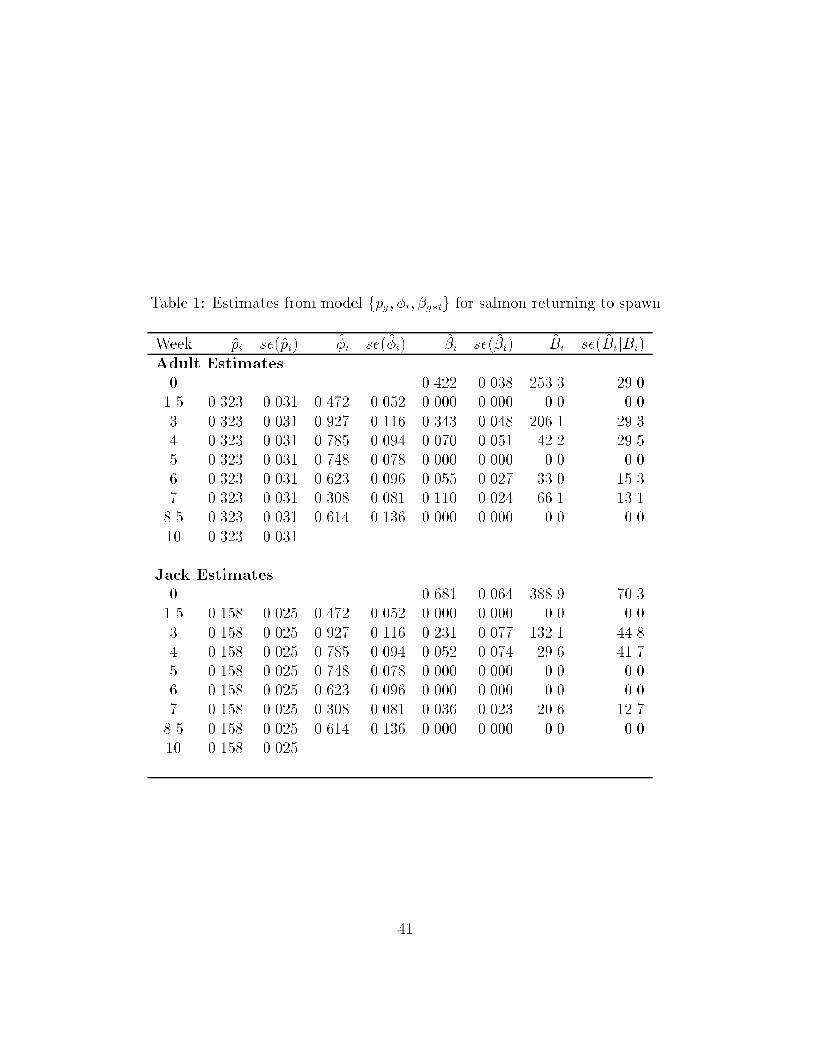
Table 1: Estimates from model fpg; �t; �g�tg for salmon returning to spawn

Week pi se(pi) �i se(�i) �i se(�i) Bi se(BijBi)Adult Estimates

0 0.422 0.038 253.3 29.01.5 0.323 0.031 0.472 0.052 0.000 0.000 0.0 0.03 0.323 0.031 0.927 0.116 0.343 0.048 206.1 29.34 0.323 0.031 0.785 0.094 0.070 0.051 42.2 29.55 0.323 0.031 0.748 0.078 0.000 0.000 0.0 0.06 0.323 0.031 0.623 0.096 0.055 0.027 33.0 15.37 0.323 0.031 0.308 0.081 0.110 0.024 66.1 13.18.5 0.323 0.031 0.614 0.136 0.000 0.000 0.0 0.010 0.323 0.031

Jack Estimates

0 0.681 0.064 388.9 70.31.5 0.158 0.025 0.472 0.052 0.000 0.000 0.0 0.03 0.158 0.025 0.927 0.116 0.231 0.077 132.1 44.84 0.158 0.025 0.785 0.094 0.052 0.074 29.6 41.75 0.158 0.025 0.748 0.078 0.000 0.000 0.0 0.06 0.158 0.025 0.623 0.096 0.000 0.000 0.0 0.07 0.158 0.025 0.308 0.081 0.036 0.023 20.6 12.78.5 0.158 0.025 0.614 0.136 0.000 0.000 0.0 0.010 0.158 0.025

41

Table 2: Estimates of age-speci�c breeding proportions from �tting two mod-els with capture-probabilities a linear function of the number of visits of Ta-ble 4 of Clobert et al. (1994), breeding restricted to ages 2-5, and survival isconstant over time and among cohorts.

Each cohort allowed its own Common breeding Common breedingbreeding proportions proportions for proportions using

Cohort 1 Cohort 2 Cohort 3 all cohorts Pradel's Age Est sec Est sec Est sec Est se Est se

2 .240 .169 .000 - .401 .181 .299 .124 .214 .1133 .339 .219 .553 .249 .214 .201 .356 .173 .316 .1654 .000 - .293 .314 .000 - .001 .161 .001 .1775 .422 .179 .155 .269 .385 .151 .344 .120 .470 .162

Average 3.604 .426 3.602 .413 3.370 .393 3.390 .296 3.727 .378

b�a .808 .064 .808 .064 .808 .064 .806 .064 .806 .064

b�b0 .076 .024 .109 .035 .094 .027 .091 .024

log-likelihood -185.1 -187.2a Survival probability for breedersb Survival probability from the time of marking at age 0 to the �rst age ofbreeding.c Standard errors are not available when estimates of age-speci�c breedingproportions fall on the boundary of the parameter space - refer to Schwarzand Arnason (1996) for details.

42

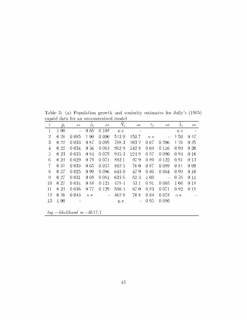
Table 3: (a) Population growth and seniority estimates for Jolly's (1965)capsid data for an unconstrained model.

i pi se �i se Ni se i se �i se1 1.00 - 0.65 0.108 n.e. - n.e -2 0.28 0.085 1.00 0.000 513.9 150.7 n.e - 1.50 0.473 0.22 0.033 0.87 0.095 768.3 103.2 0.67 0.206 1.26 0.254 0.22 0.034 0.56 0.063 962.9 142.8 0.69 0.116 0.99 0.205 0.23 0.033 0.84 0.075 945.3 124.9 0.57 0.090 0.94 0.166 0.24 0.029 0.79 0.071 882.1 97.9 0.89 0.122 0.91 0.137 0.31 0.033 0.65 0.057 802.5 76.0 0.87 0.089 0.81 0.098 0.27 0.025 0.99 0.096 643.0 47.9 0.80 0.064 0.99 0.109 0.27 0.031 0.69 0.081 633.6 62.3 1.00 - 0.76 0.1110 0.27 0.034 0.88 0.121 478.4 53.1 0.91 0.065 1.06 0.1811 0.24 0.036 0.77 0.129 506.4 67.0 0.83 0.071 0.92 0.1812 0.26 0.043 n.e. - 462.8 70.8 0.84 0.078 n.e. -13 1.00 - n.e. - 0.95 0.080

log � likelihood = �3117:1

43

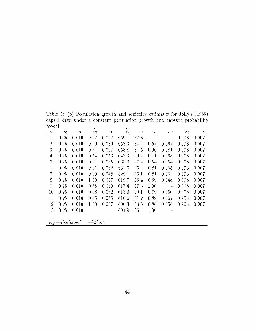
Table 3: (b) Population growth and seniority estimates for Jolly's (1965)capsid data under a constant population growth and capture probabilitymodel.i pi se �i se Ni se i se �i se

1 0.25 0.010 0.57 0.067 659.7 37.3 0.998 0.0072 0.25 0.010 0.90 0.080 658.3 34.2 0.57 0.067 0.998 0.0073 0.25 0.010 0.71 0.067 653.8 31.5 0.90 0.081 0.998 0.0074 0.25 0.010 0.54 0.053 647.3 29.2 0.71 0.068 0.998 0.0075 0.25 0.010 0.81 0.065 638.9 27.4 0.54 0.054 0.998 0.0076 0.25 0.010 0.81 0.062 631.5 26.4 0.81 0.065 0.998 0.0077 0.25 0.010 0.69 0.048 628.1 26.1 0.81 0.062 0.998 0.0078 0.25 0.010 1.00 0.007 619.7 26.4 0.69 0.048 0.998 0.0079 0.25 0.010 0.78 0.050 617.4 27.5 1.00 - 0.998 0.00710 0.25 0.010 0.88 0.062 613.0 29.1 0.79 0.050 0.998 0.00711 0.25 0.010 0.86 0.056 610.6 31.2 0.89 0.062 0.998 0.00712 0.25 0.010 1.00 0.007 606.3 33.6 0.86 0.056 0.998 0.00713 0.25 0.010 604.9 36.4 1.00 -

log � likelihood = �3236:4

44

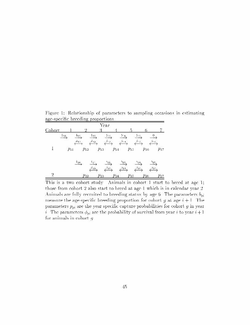
Figure 1: Relationship of parameters to sampling occasions in estimatingage-speci�c breeding proportions

YearCohort 1 2 3 4 5 6 7

b10�!b11�!

b12�!b13�!

b14�!b15�!

0�!

�11 !�12 !

�13 !�14 !

�15 !�16 !

1 p11 p12 p13 p14 p15 p16 p17

b20�!b21�!

b22�!b23�!

b24�!b25�!

�22 !�23 !

�24 !�25 !

�26 !2 p22 p23 p24 p25 p26 p27

This is a two cohort study. Animals in cohort 1 start to breed at age 1;those from cohort 2 also start to breed at age 1 which is in calendar year 2.Animals are fully recruited to breeding status by age 6. The parameters bgimeasure the age-speci�c breeding proportion for cohort g at age i + 1. Theparameters pgi are the year speci�c capture probabilities for cohort g in yeari. The parameters �gi are the probability of survival from year i to year i+1for animals in cohort g.

45