Angular Propagation Descriptions Relevant for Base Station Adaptive Antenna …kom.aau.dk/~pe/education/phd/litt/kluwer1999.pdf · 2004-07-21 · changes in the partial selection

Wireless Personal Communications11: 3–29, 1999.© 1999Kluwer Academic Publishers. Printed in the Netherlands.

Angular Propagation Descriptions Relevantfor Base Station Adaptive Antenna Operations∗

PATRICK C.F. EGGERSCenter for PersonKommunikation, Aalborg University, Fredrik Bajersvej 7A-5, DK-9220 Aalborg, DenmarkE-mail: [email protected]

Abstract. This paper presents basic short-term angular domain propagation descriptions relevant for beam-oriented SDMA operations, i.e. for spatially based algorithms, contrary to temporally based. A distinction ismade between angular variant and invariant situations, i.e. whether the antenna system radiation pattern remainsunchanged or not when sweeping over the angular domain. For the angular invariant case, multibeam diversityrelations are explained, as well as simple data enhancement techniques for measurement refinements. For theangular variant case using linear arrays, this paper suggests a representation in the invariant virtual Dopplerdomain. A key benefit of generating beams in the Doppler domain instead of directly in the angular domain isa substantial saving in numerical complexity.

Keywords: angular propagation, angular modelling, DOA, adaptive antennas, SDMA.

1. Introduction

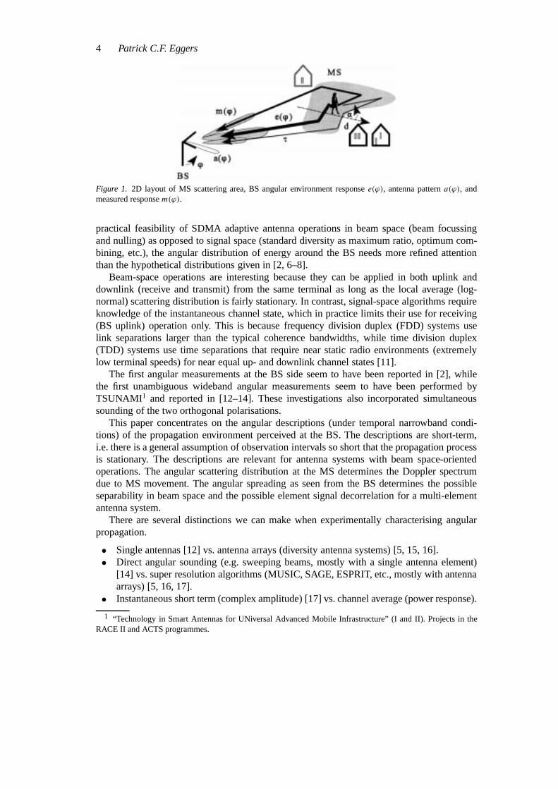
The angular distribution of scattered energy around a mobile terminal is well described whenconsidering the mobile station (MS) end, see Figure 1. Statistical descriptions of received RFamplitude, phase, and derivatives have been linked with 2D angular scattering models [1, 2].Measurements have also been performed displaying the angular scattering distributions for anMS in urban areas [3–5].

However, descriptions of outdoor radio environments at the base station (BS) end (see Fig-ure 1) have mainly been focussed on the branch cross-correlation properties of multi-antennaelement systems. The outdoor environment is described by the spatial cross-correlationsR12

via measurements (space diversity) and modelled by the associated spatial auto-correlationfunctionsRBS(1x) [2, 6] (see Section 2.5 for definitions). These auto-correlations are basedon simplistic physical models of the scattering scenarios around the MS [2, 6–8] and theirrelation to the BS.

Narrow beam adaptive antennas can be used to suppress interference by spatial filteringand for range extension through increased gain [9]. This can be applied in existing mobilesystems where each user in a sector has a unique channel in the temporal (frequency, timeslot) or code domains. In an SDMA operation, the spatial domain is used for multiple access,such that several users can share the same temporal and code channels [9, 10]. In its simplestform, SDMA can operate just using sector partitioning, implemented with a grid of beams foreach user.

Few accounts on descriptive and practical work regarding accurate angular signal distri-butions at the BS have been given in the classic literature. With the increased interest and

∗ Parts of this paper have been previously presented in [18, 19, and 25]

4 Patrick C.F. Eggers

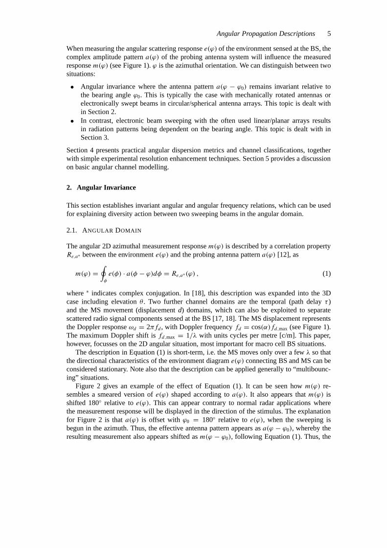
Figure 1. 2D layout of MS scattering area, BS angular environment responsee(ϕ), antenna patterna(ϕ), andmeasured responsem(ϕ).

practical feasibility of SDMA adaptive antenna operations in beam space (beam focussingand nulling) as opposed to signal space (standard diversity as maximum ratio, optimum com-bining, etc.), the angular distribution of energy around the BS needs more refined attentionthan the hypothetical distributions given in [2, 6–8].

Beam-space operations are interesting because they can be applied in both uplink anddownlink (receive and transmit) from the same terminal as long as the local average (log-normal) scattering distribution is fairly stationary. In contrast, signal-space algorithms requireknowledge of the instantaneous channel state, which in practice limits their use for receiving(BS uplink) operation only. This is because frequency division duplex (FDD) systems uselink separations larger than the typical coherence bandwidths, while time division duplex(TDD) systems use time separations that require near static radio environments (extremelylow terminal speeds) for near equal up- and downlink channel states [11].

The first angular measurements at the BS side seem to have been reported in [2], whilethe first unambiguous wideband angular measurements seem to have been performed byTSUNAMI1 and reported in [12–14]. These investigations also incorporated simultaneoussounding of the two orthogonal polarisations.

This paper concentrates on the angular descriptions (under temporal narrowband condi-tions) of the propagation environment perceived at the BS. The descriptions are short-term,i.e. there is a general assumption of observation intervals so short that the propagation processis stationary. The descriptions are relevant for antenna systems with beam space-orientedoperations. The angular scattering distribution at the MS determines the Doppler spectrumdue to MS movement. The angular spreading as seen from the BS determines the possibleseparability in beam space and the possible element signal decorrelation for a multi-elementantenna system.

There are several distinctions we can make when experimentally characterising angularpropagation.

• Single antennas [12] vs. antenna arrays (diversity antenna systems) [5, 15, 16].• Direct angular sounding (e.g. sweeping beams, mostly with a single antenna element)

[14] vs. super resolution algorithms (MUSIC, SAGE, ESPRIT, etc., mostly with antennaarrays) [5, 16, 17].

• Instantaneous short term (complex amplitude) [17] vs. channel average (power response).

1 “Technology in Smart Antennas for UNiversal Advanced Mobile Infrastructure” (I and II). Projects in theRACE II and ACTS programmes.

Angular Propagation Descriptions 5

When measuring the angular scattering responsee(ϕ) of the environment sensed at the BS, thecomplex amplitude patterna(ϕ) of the probing antenna system will influence the measuredresponsem(ϕ) (see Figure 1).ϕ is the azimuthal orientation. We can distinguish between twosituations:

• Angular invariance where the antenna patterna(ϕ − ϕ0) remains invariant relative tothe bearing angleϕ0. This is typically the case with mechanically rotated antennas orelectronically swept beams in circular/spherical antenna arrays. This topic is dealt within Section 2.

• In contrast, electronic beam sweeping with the often used linear/planar arrays resultsin radiation patterns being dependent on the bearing angle. This topic is dealt with inSection 3.

Section 4 presents practical angular dispersion metrics and channel classifications, togetherwith simple experimental resolution enhancement techniques. Section 5 provides a discussionon basic angular channel modelling.

2. Angular Invariance

This section establishes invariant angular and angular frequency relations, which can be usedfor explaining diversity action between two sweeping beams in the angular domain.

2.1. ANGULAR DOMAIN

The angular 2D azimuthal measurement responsem(ϕ) is described by a correlation propertyRe,a∗ between the environmente(ϕ) and the probing antenna patterna(ϕ) [12], as

m(ϕ) =∮φ

e(φ) · a(φ − ϕ)dφ = Re,a∗(ϕ) , (1)

where∗ indicates complex conjugation. In [18], this description was expanded into the 3Dcase including elevationθ . Two further channel domains are the temporal (path delayτ )and the MS movement (displacementd) domains, which can also be exploited to separatescattered radio signal components sensed at the BS [17, 18]. The MS displacement representsthe Doppler responseωd = 2πfd , with Doppler frequencyfd = cos(α)fd,max (see Figure 1).The maximum Doppler shift isfd,max = 1/λ with units cycles per metre [c/m]. This paper,however, focusses on the 2D angular situation, most important for macro cell BS situations.

The description in Equation (1) is short-term, i.e. the MS moves only over a fewλ so thatthe directional characteristics of the environment diagrame(ϕ) connecting BS and MS can beconsidered stationary. Note also that the description can be applied generally to “multibounc-ing” situations.

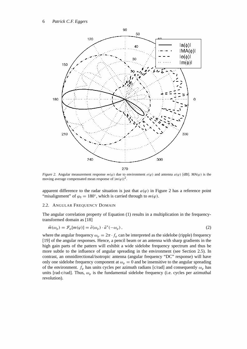
Figure 2 gives an example of the effect of Equation (1). It can be seen howm(ϕ) re-sembles a smeared version ofe(ϕ) shaped according toa(ϕ). It also appears thatm(ϕ) isshifted 180◦ relative toe(ϕ). This can appear contrary to normal radar applications wherethe measurement response will be displayed in the direction of the stimulus. The explanationfor Figure 2 is thata(ϕ) is offset withϕ0 = 180◦ relative toe(ϕ), when the sweeping isbegun in the azimuth. Thus, the effective antenna pattern appears asa(ϕ − ϕ0), whereby theresulting measurement also appears shifted asm(ϕ − ϕ0), following Equation (1). Thus, the


Figure 2. Angular measurement responsem(ϕ) due to environmente(ϕ) and antennaa(ϕ) [dB]. MA(ϕ) is themoving average compensated mean response of|m(ϕ)|2.

apparent difference to the radar situation is just thata(ϕ) in Figure 2 has a reference point“misalignment” ofϕ0 = 180◦, which is carried through tom(ϕ).

2.2. ANGULAR FREQUENCY DOMAIN

The angular correlation property of Equation (1) results in a multiplication in the frequency-transformed domain as [18]

m(ωϕ) = Fϕ[m(ϕ)] = e(ωϕ) · a∗(−ωϕ) , (2)

where the angular frequencyωϕ = 2π ·fϕ can be interpreted as the sidelobe (ripple) frequency[19] of the angular responses. Hence, a pencil beam or an antenna with sharp gradients in thehigh gain parts of the pattern will exhibit a wide sidelobe frequency spectrum and thus bemore subtle to the influence of angular spreading in the environment (see Section 2.5). Incontrast, an omnidirectional/isotropic antenna (angular frequency “DC” response) will haveonly one sidelobe frequency component atωϕ = 0 and be insensitive to the angular spreadingof the environment.fϕ has units cycles per azimuth radians [c/rad] and consequentlyωϕ hasunits [rad·c/rad]. Thus,ωϕ is the fundamental sidelobe frequency (i.e. cycles per azimuthalrevolution).


2.3. AVERAGE POWER RESPONSE

Under uncorrelated scattering (US) conditions, the voltage summation in the integral in Equa-tion (1) will be noncoherent, whereby the same angular correlation property will hold for theaverage power responsesA(ϕ) = |a(ϕ)|2,M(ϕ) = |m(ϕ)|2 andE(ϕ) = |e(ϕ)|2 [18], i.e.

M(ϕ) = |m(ϕ)|2 =∮φ

E(φ) ·A(φ − ϕ)dφ = RE,A(ϕ) . (3)

The free space antenna patterna(ϕ) is deterministic and thus does not require any averagingto establish the power response. The averaging can be performed in either the spatial (MSmovement) or the temporal domain. Spatial averaging assumes a certain area around the MSwhere the angular distribution in Equation (1) is stationary. This will typically correspondto intervals having constant total average power as a function of MS movement, i.e. no log-normal fading. Temporal averaging assumes a sounding bandwidth larger than the coherencebandwidth of the channel [12, 13], as the process can be interpreted as averaging over thefrequency domain fades. Consequently, a frequency interval covering a sufficient number offrequency domain fades is needed to provide a statistically sound estimate of the mean.

2.4. ANGULAR TEMPORAL DOMAIN ANALOGIES

With the convolution (⊗) relationmτ (τ) = h(τ) ⊗ eτ (τ ) in the temporal domain betweensystemh(τ) and environmenteτ (τ ) – and the correlation relation in the angular domain(a(ϕ)

ande(ϕ)), several analogies between the two domains exist. One analogy is between meanangle jitter and mean delay jitter, both due to dynamics in the channel caused by the MSmovement [19].

2.5. CORRELATION FUNCTIONS

Assuming a wide sense stationary (WSS) fading process in the angular domain, we can estab-lish angular fading correlation functions [18]. Note that such functions are different from thesystem response relations of Equations (1) and (3).

Angular fading is the third fading process (complex amplitude changes of the receivedsignal due to beam sweeping) apart from traditional temporal (due to multipath) and spatial(due to MS movement) domain fading [2, 20]. We can define angular domain fading as antennafading where the terminals (MS and BS) are spatially static. The fading is then caused bychanges in the partial selection of the angular environment responsee(ϕ), due to selectivity inamplitude or phase by the antenna patterna(ϕ), when sweepinga(ϕ) over the angular domain.As an analogy, we can regard the antenna as an angular filter causing interference betweenangular components appearing within its beam width. Even an omnidirectional antenna canprovide angular fading if the antenna has a phase response that changes sufficiently over theangular region spanned by the environment response.

The correlation functions can be normalised to form correlation coefficient functions,ρ = C/C(0) for the auto-correlations andρ12 = C12/

√(C11(0) · C22(0)) for the cross-

correlations.C12 = R12− µ1 · µ∗2 is the cross-variance andµn = E[rn] the mean value. Thecross-correlation isR12 = E[r1·r∗2 ], whereE[•] is the expectation value operator. For a contin-uous random variabler with probability density distribution (pfd)f (r), E[r] = ∫ r · f (r) dr.For example, ifr1 andr2 are the complex envelopes of two received antenna branch signals due


to a moving and transmitting MS,R12 would be the signal cross-correlation of the antenna sys-tem. The correlation coefficient functions are used to define coherence measures as separationwidths/lengths (1x), where the correlation reaches a reference level, i.e.1x|ρ(1x)=reference.The coherence widths/lengths (1x) can then be used for setting coarse limits for worthwhilediversity action. For example, ifr(x) represents the complex envelope along the antenna sepa-ration axisx in a space diversity system, then the auto-correlationRBS(1x) = e[r(x)·r(1x)∗]will represent the signal cross-correlation just likeR12 of two antennas spaced with1x [2, 6].

To separate different domain effects, we can distinguish between

• Angular diversity: Spatially fixed terminals, with the BS antenna system sweeping two ormore beams in the angular domain, under temporal/spatial static channel conditions. Theoperations can be applied to both the instantaneous and the average responses. The beamsare narrow and function selectively on the environment response. A possible applicationis for transportable terminals in a wireless local area network (WLAN).

• Traditional antenna diversity: Spatially moving terminal(s) with fixed antenna systemsyielding temporal/spatial dynamical channel conditions. Fixed decorrelation in the an-gular domain is possible via (angle, pattern, space) diversity as used in mobile radionetworks. Note that these diversity combiner operations can be transformed back intoan instantaneously dynamically changing antenna diagram. However, it differs from theangular diversity above in that the antenna beamwidths are wide and often illuminate thewhole environment response. This can result in requirements of fast algorithm updating.

• Adaptive antenna diversity: A merging of the first two diversity types. Channel dynamicsappear due to MS movement, while the beams at the same time sweep in the angulardomain. Due to the selective narrow beams, a lowering of MS Doppler responses andtemporal dispersion can result, relaxing the updating speed of the algorithms. Due tofading processes in both the angular and the MS spatial domain, an extra degree offreedom exists which can be utilised for further optimisation of combining algorithms.

Traditional SDMA is thought of as a single beam-former (BF)/antenna system, operating on auser and some interferers. Angular and adaptive antenna diversity means that several (in thispaper for simplicity two) BF/antenna systems are applied to a user and some interferers. An-other distinction is that traditional antenna diversity is normally implemented with two singleantenna elements, while angular and adaptive antenna diversity can be applied with distributedantenna array systems. All of the mentioned diversity types, however, can be grouped togetherunder the general term antenna diversity [20].

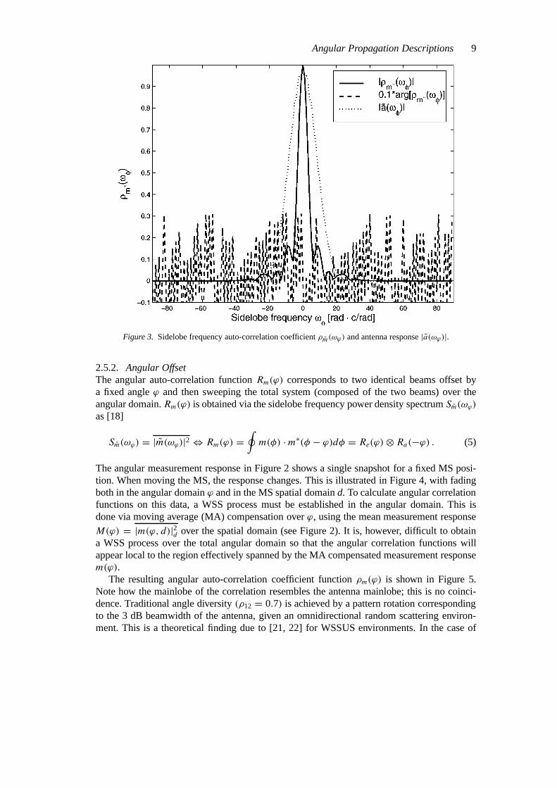
2.5.1. Sidelobe Frequency OffsetIf we consider the average measurement response from Equation (3), we get via the Wiener-Kitchine correlation theorem [18]

M(ϕ) = |m(ϕ)|2⇔ Rm(ωϕ) =∮m(ωφ) · m∗(ωφ − ωϕ)dωϕ

= M(ωϕ) = E(ωϕ) · A∗(ωϕ) = Re(ωϕ) · R∗a (ωϕ ,(4)

where the frequency (Fourier) transformation is indicated by “⇔”. Rm(ωϕ) is the sidelobefrequency domain auto-correlation.ρm(ωϕ) is shown in Figure 3 for the case of Figure 2.


Figure 3. Sidelobe frequency auto-correlation coefficientρm(ωϕ) and antenna response|a(ωϕ)|.

2.5.2. Angular OffsetThe angular auto-correlation functionRm(ϕ) corresponds to two identical beams offset bya fixed angleϕ and then sweeping the total system (composed of the two beams) over theangular domain.Rm(ϕ) is obtained via the sidelobe frequency power density spectrumSm(ωϕ)

as [18]

Sm(ωϕ) = |m(ωϕ)|2⇔ Rm(ϕ) =∮m(φ) ·m∗(φ − ϕ)dφ = Re(ϕ)⊗ Ra(−ϕ) . (5)

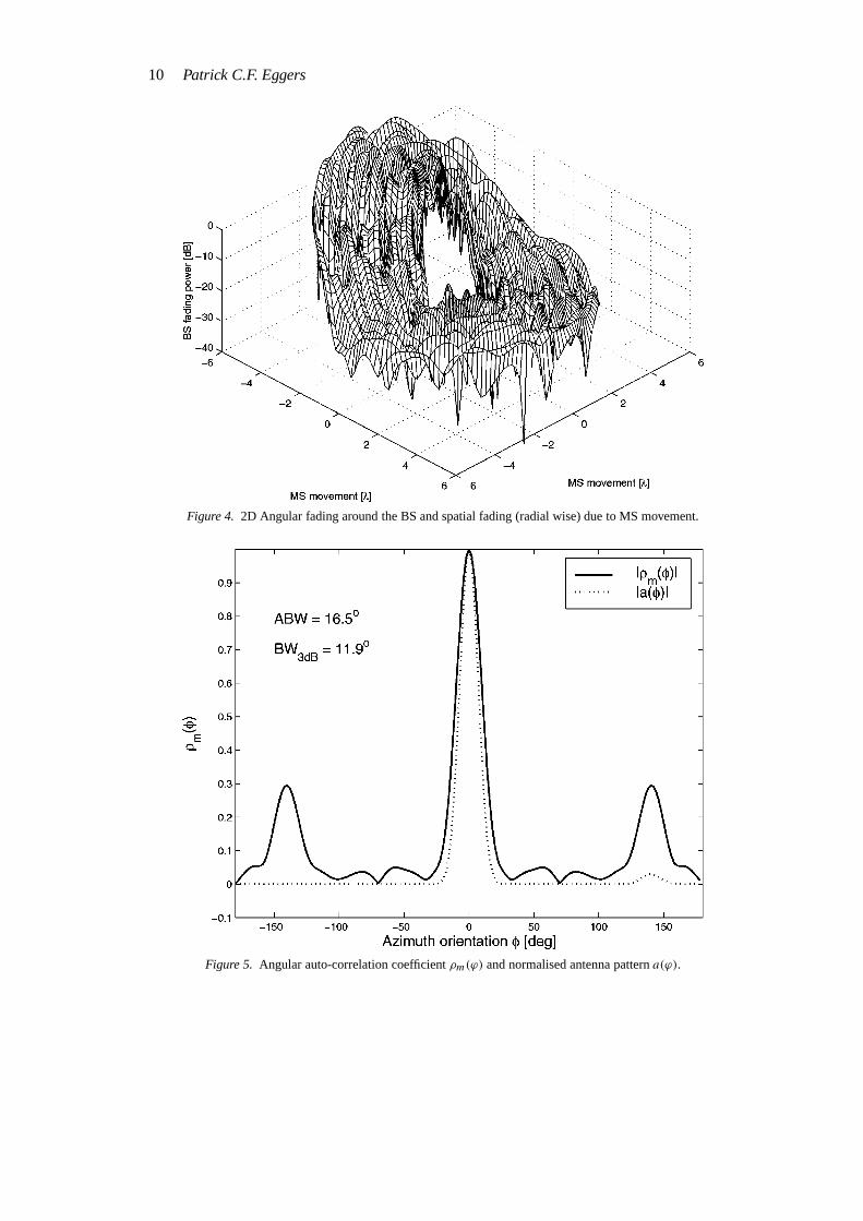
The angular measurement response in Figure 2 shows a single snapshot for a fixed MS posi-tion. When moving the MS, the response changes. This is illustrated in Figure 4, with fadingboth in the angular domainϕ and in the MS spatial domaind. To calculate angular correlationfunctions on this data, a WSS process must be established in the angular domain. This isdone via moving average (MA) compensation overϕ, using the mean measurement responseM(ϕ) = |m(ϕ, d)|2d over the spatial domain (see Figure 2). It is, however, difficult to obtaina WSS process over the total angular domain so that the angular correlation functions willappear local to the region effectively spanned by the MA compensated measurement responsem(ϕ).

The resulting angular auto-correlation coefficient functionρm(ϕ) is shown in Figure 5.Note how the mainlobe of the correlation resembles the antenna mainlobe; this is no coinci-dence. Traditional angle diversity(ρ12 = 0.7) is achieved by a pattern rotation correspondingto the 3 dB beamwidth of the antenna, given an omnidirectional random scattering environ-ment. This is a theoretical finding due to [21, 22] for WSSUS environments. In the case of


Figure 4. 2D Angular fading around the BS and spatial fading (radial wise) due to MS movement.

Figure 5. Angular auto-correlation coefficientρm(ϕ) and normalised antenna patterna(ϕ).


Figures 2 and 4, the angular coherence beamwidth(ABW= ϕ|ρm(ϕ)=0.7) is 16.5◦ and the 3 dBbeamwidth of the antenna is 11.9◦ (see Figure 5).

Note in Figure 2 that the fundamental frequency of the angular fading corresponds to themainlobe of the antenna (which has a constant phase response). If the antenna had a morerandom phase response, the environment could become a determining factor in the angularfading rate.

The ABW is representative for two beam diversity (equal pattern, phase centres) in theangular domain. Note also that if these angular correlations(Rm12) were applied to twoantennas separated by1x, Rm12(ϕ = 0)|1x 6= RBS(1x) and therefore do not correspondto the traditional diversity case with fixed beams(RBS). This is due to the two correlationsreferring to different fading domains (angular due to beam sweeping and spatial due to MSmovement).Rm12(ϕ = 0) is the case of two simultaneously sweeping beams with no angularoffset between them.

2.5.3. Pattern ShapeIn the case of two different antenna patterns, we get

M12(ϕ) = m1(ϕ) ·m∗2(ϕ)⇔ Rm12(ωϕ) =∮m1(ωϕ) · m∗2(ωφ − ωϕ)dωφ = M12(ωϕ) , (6)

where the angular measurement response dependent on antenna “n” ismn(ϕ) = R∗e,an(ϕ) =∮e(φ) · an(φ − ϕ)dφ ⇔ mn(ωϕ) = e(ωϕ) · a∗n(−ωϕ). The sidelobe frequency cross-spectral

densitySm12(ωϕ) yields the angular cross-correlation function as

Sm12(ωϕ) = m1(ωϕ) · m∗2(ωϕ)⇔ Rm12(ϕ) =∮m1(φ) ·m∗2(φ − ϕ)dφ . (7)

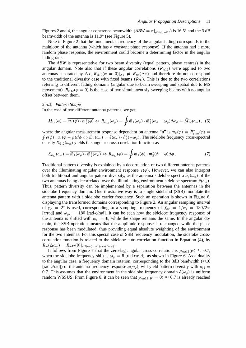
Traditional pattern diversity is explained by a decorrelation of two different antenna patternsover the illuminating angular environment responsee(ϕ). However, we can also interpretboth traditional and angular pattern diversity, as the antenna sidelobe spectraan(ωϕ) of thetwo antennas being decorrelated over the illuminating environment sidelobe spectrume(ωϕ).Thus, pattern diversity can be implemented by a separation between the antennas in thesidelobe frequency domain. One illustrative way is to single sideband (SSB) modulate theantenna pattern with a sidelobe carrier frequency. Such an operation is shown in Figure 6,displaying the transformed domains corresponding to Figure 2. An angular sampling intervalof ϕs = 2◦ is used, corresponding to a sampling frequency offϕs = 1/ϕs = 180/2π[c/rad] andωϕs = 180 [rad·c/rad]. It can be seen how the sidelobe frequency response ofthe antenna is shifted withωϕ = 8, while the shape remains the same. In the angular do-main, the SSB operation means that the amplitude response is unchanged while the phaseresponse has been modulated, thus providing equal absolute weighting of the environmentfor the two antennas. For this special case of SSB frequency modulation, the sidelobe cross-correlation function is related to the sidelobe auto-correlation function in Equation (4), byRm(1ωϕ) = Rm12(0)|m2(ωϕ)=m1(ωϕ+1ωϕ).

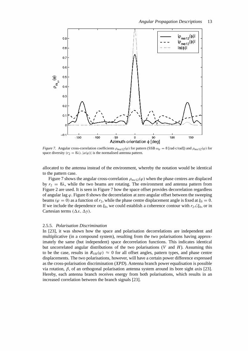
It follows from Figure 7 that the zero-lag angular cross-correlation isρma12(ϕ) ≈ 0.7,when the sidelobe frequency shift isωϕ = 8 [rad·c/rad], as shown in Figure 6. As a dualityto the angular case, a frequency domain rotation, corresponding to the 3dB bandwidth (≈16[rad·c/rad]) of the antenna frequency responsea(ωϕ), will yield pattern diversity withρ12 =0.7. This assumes that the environment in the sidelobe frequency domaine(ωϕ) is uniformrandom WSSUS. From Figure 8, it can be seen thatρma12(ϕ = 0) ≈ 0.7 is already reached


Figure 6. Sidelobe frequency spectra [dB]. Antennaa2(ωϕ) is a sidelobe frequency SSB modulated version ofa(ωϕ). e(ωϕ) is the environmental response.

for an SSB shift of approximately 8 [rad·c/rad]. This may be becausee(ωϕ) is not uniform,thereby causing a higher degree of decorrelation.

Note though that for general pattern diversity, we are not restricted to the changing of theantenna phase response. It is the total complex amplitude response of the antennas, that consti-tutes pattern difference. This pattern difference is easily visualised in the sidelobe frequencydomain.

2.5.4. Space OffsetIf the phase centres of the antennas are offset, we can interpret this as a phase shift process ofthe angular environment response [18], i.e.

e2(ϕ, θ) = e(ϕ, θ) · t (ϕ, θ); t (ϕ, θ) = ej ·k·r2·cos(ξ)

cos(ξ) = x · x2+ y · y2+ z · z2; k = 2·πλ,

(8)

wherex, y, andz are the Cartesian coordinates on the unit sphere. No suffix indicates theenvironment direction and suffix 2 represents the translated position.r2]ξ is the displacementvector (of the two antenna phase centres) with angle relative to the environment directionϕ.

The angular correlation expressions due to space offset are the same as the ones given in theprevious pattern case in Equations (6) and (7), except for the different measurement responsesthat stem from different environment diagrams, i.e.mn(ϕ) = Ren,a∗(ϕ) =

∮en(φ) · a(φ −

ϕ)dφ ⇔ mn(ωϕ) = en(ωϕ) · a∗(−ωϕ). In principle, the spatial phase centre offset could be


Figure 7. Angular cross-correlation coefficientsρma12(ϕ) for pattern (SSBωϕ = 8 [rad·c/rad]) andρme12(ϕ) forspace diversity(r2 = 8λ). |a(ϕ)| is the normalised antenna pattern.

allocated to the antenna instead of the environment, whereby the notation would be identicalto the pattern case.

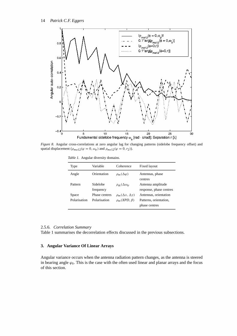
Figure 7 shows the angular cross-correlationρme12(ϕ)when the phase centres are displacedby r2 = 8λ, while the two beams are rotating. The environment and antenna pattern fromFigure 2 are used. It is seen in Figure 7 how the space offset provides decorrelation regardlessof angular lagϕ. Figure 8 shows the decorrelation at zero angular offset between the sweepingbeams(ϕ = 0) as a function ofr2, while the phase centre displacement angle is fixed atξ0 = 0.If we include the dependence onξ0, we could establish a coherence contour withr2]ξ0, or inCartesian terms(1x,1y).

2.5.5. Polarisation DiscriminationIn [23], it was shown how the space and polarisation decorrelations are independent andmultiplicative (in a compound system), resulting from the two polarisations having approx-imately the same (but independent) space decorrelation functions. This indicates identicalbut uncorrelated angular distributions of the two polarisations (V andH ). Assuming thisto be the case, results inRVH(ϕ) ≈ 0 for all offset angles, pattern types, and phase centredisplacements. The two polarisations, however, will have a certain power difference expressedas the cross-polarisation discrimination (XPD). Antenna branch power equalisation is possiblevia rotation,β, of an orthogonal polarisation antenna system around its bore sight axis [23].Hereby, each antenna branch receives energy from both polarisations, which results in anincreased correlation between the branch signals [23].


Figure 8. Angular cross-correlations at zero angular lag for changing patterns (sidelobe frequency offset) andspatial displacement (ρma12(ϕ = 0, ωϕ) andρme12(ϕ = 0, r2)).

Table 1. Angular diversity domains.

Type Variable Coherence Fixed layout

Angle Orientation ρm(1ϕ) Antennas, phase

centres

Pattern Sidelobe ρm(1ωϕ Antenna amplitude

frequency response, phase centres

Space Phase centresρm(1x,1y) Antennas, orientation

Polarisation Polarisation ρm(XPD, β) Patterns, orientation,

phase centres

2.5.6. Correlation SummaryTable 1 summarises the decorrelation effects discussed in the previous subsections.

3. Angular Variance Of Linear Arrays

Angular variance occurs when the antenna radiation pattern changes, as the antenna is steeredin bearing angleϕ0. This is the case with the often used linear and planar arrays and the focusof this section.


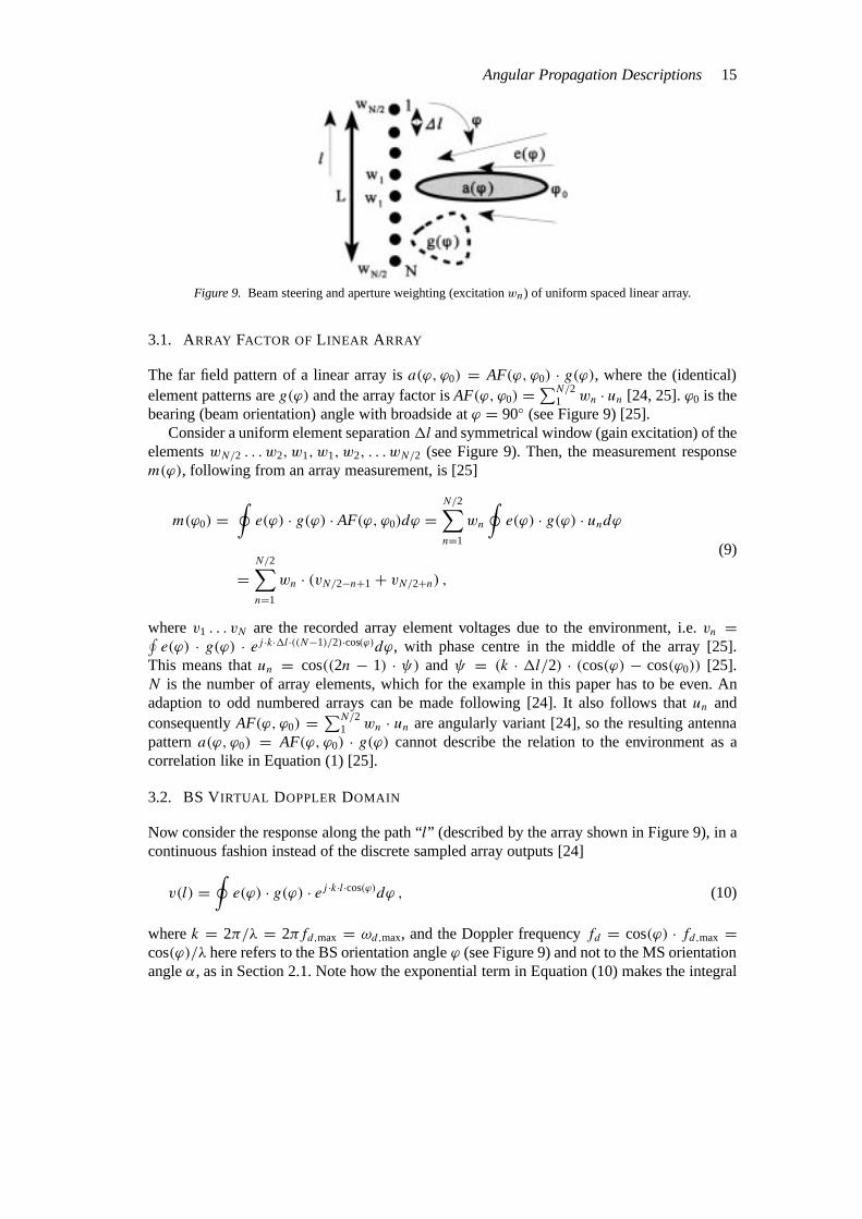
Figure 9. Beam steering and aperture weighting (excitationwn) of uniform spaced linear array.

3.1. ARRAY FACTOR OFLINEAR ARRAY

The far field pattern of a linear array isa(ϕ, ϕ0) = AF(ϕ, ϕ0) · g(ϕ), where the (identical)element patterns areg(ϕ) and the array factor isAF(ϕ, ϕ0) =∑N/2

1 wn · un [24, 25].ϕ0 is thebearing (beam orientation) angle with broadside atϕ = 90◦ (see Figure 9) [25].

Consider a uniform element separation1l and symmetrical window (gain excitation) of theelementswN/2 . . . w2, w1, w1, w2, . . . wN/2 (see Figure 9). Then, the measurement responsem(ϕ), following from an array measurement, is [25]

m(ϕ0) =∮e(ϕ) · g(ϕ) · AF(ϕ, ϕ0)dϕ =

N/2∑n=1

wn

∮e(ϕ) · g(ϕ) · undϕ

=N/2∑n=1

wn · (vN/2−n+1 + vN/2+n) ,(9)

wherev1 . . . vN are the recorded array element voltages due to the environment, i.e.vn =∮e(ϕ) · g(ϕ) · ej ·k·1l·((N−1)/2)·cos(ϕ)dϕ, with phase centre in the middle of the array [25].

This means thatun = cos((2n − 1) · ψ) andψ = (k · 1l/2) · (cos(ϕ) − cos(ϕ0)) [25].N is the number of array elements, which for the example in this paper has to be even. Anadaption to odd numbered arrays can be made following [24]. It also follows thatun andconsequentlyAF(ϕ, ϕ0) = ∑N/2

1 wn · un are angularly variant [24], so the resulting antennapatterna(ϕ, ϕ0) = AF(ϕ, ϕ0) · g(ϕ) cannot describe the relation to the environment as acorrelation like in Equation (1) [25].

3.2. BS VIRTUAL DOPPLERDOMAIN

Now consider the response along the path “l” (described by the array shown in Figure 9), in acontinuous fashion instead of the discrete sampled array outputs [24]

v(l) =∮e(ϕ) · g(ϕ) · ej ·k·l·cos(ϕ)dϕ , (10)

wherek = 2π/λ = 2πfd,max = ωd,max, and the Doppler frequencyfd = cos(ϕ) · fd,max =cos(ϕ)/λ here refers to the BS orientation angleϕ (see Figure 9) and not to the MS orientationangleα, as in Section 2.1. Note how the exponential term in Equation (10) makes the integral


much like a Fourier transform and consequently a variable transform fromϕ to ωd = 2π ·cos(ϕ)/λ results in [25]

v(l) =∫e(ωd) · g(ωd) · ej ·ωd ·ldωd = F −1[v(ωd)] , (11)

where

v(ωd) = e(ωd) · g(ωd) = e(ϕ) · g(ϕ)√ω2d,max− ω2

d

(12)

andϕ = arccos(ωd/ωd,max) [2, 25]. v(ωd) is the virtual Doppler spectrum [2, 25] of theenvironment and antenna element at the BS, due to a virtual movement of the antenna elementalong the path given by the antenna array (see Figure 9). This Doppler domain should notbe confused with the MS referenced Doppler domain [26], as only the latter introduces realspatially (temporally) dependent channel dynamics on the link between MS and BS.

In the case of a linear array, a finite window lengthL is inherently imposed onv(l). Forsimplicity, we describe this windoww(l) as external. Thus, the measured response due tothe virtual movement ism(l) = v(l) · w(l) and the corresponding Doppler spectrum for theenvironment and total antenna system is

m(ωd) = F [m(l)] =∫v(l) · w(l) · ejωd ·ldl = v(ωd)⊗ w(ωd) . (13)

The array element outputs are just discrete sampled versions ofv(l), with sampling interval1l and sampling frequencyωs = 2π · fs = 2π/1l. It is important to note from Equations(11), (12), and (13) that we now have an invariant relation in the Doppler domainωd . Thegeneration of steered beams in the Doppler domain is due tow(ωd) and results in a fixedshape of the Doppler spectrum (beam) regardless of the Doppler shift (bearing angle) of thespectrum. The weighting of the environment spectrume(ωd) due to the element spectrumg(ωd) is still present such that the total perceived beam may change with the bearing angle.However, widebeam array elements are often used, which can make the element weightingeffect insignificant over the angular region of interest.

Another issue regarding discrete arrays is that no significant Doppler aliasing should bepresent over the angular region of interest since wraparound alias products may introduce false“echoes”. To keep aliasing at controlled levels, [25] proposed an array sampling criterion

1l ≤ λ2·(

1− 2

N

). (14)

This allows sidelobes corresponding to the narrowest mainlobe width (ωw = 2π · fw =2π · 2/L for a rectangular windoww) of the Doppler pattern to be “absorbed” in the invisibleDoppler region [24], before wraparound aliasing into the visible region appears [24, 25]. Forlarge arrays, this approaches the Nyquistλ/2 spacing.1l basically determines the aliasinglevel on the Doppler spectrum.L = N ·1l determines the Doppler resolution as well as thealiasing level. Figure 10 shows an example of beams from an array using this criterion withomnidirectional elements, i.e.g(ϕ) = 1. It is seen that only the sidelobes are present in thevisible region, for the beam steered towards±ωs/2 = 1/(2 · 0.375λ) = 11

3ωd,max (brokencurve), i.e. the mainlobe is fully “absorbed” in the invisible region.


It is interesting to note that the Doppler domain description yields all the inter-elementstatistics of amplitude, phase, and derivatives along the path described by the array axis, byanalogy to the path signal in the MS case [27].

3.3. GRID OF BEAMS

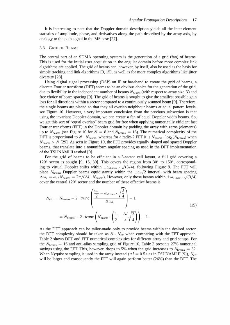
The central part of an SDMA operating system is the generation of a grid (fan) of beams.This is used for the initial user acquisition in the angular domain before more complex linkalgorithms are applied. The grid of beams can, however, by itself, also be used as the basis forsimple tracking and link algorithms [9, 15], as well as for more complex algorithms like jitterdiversity [28].

Using digital signal processing (DSP) on IF or baseband to create the grid of beams, adiscrete Fourier transform (DFT) seems to be an obvious choice for the generation of the grid,due to flexibility in the independent number of beamsNbeams(with respect to array sizeN) andfree choice of beam spacing [9]. The grid of beams is sought to give the smallest possible gainloss for all directions within a sector compared to a continuously scanned beam [9]. Therefore,the single beams are placed so that they all overlap neighbour beams at equal pattern levels,see Figure 10. However, a very important conclusion from the previous subsection is thatusing the invariant Doppler domain, we can create a fan of equal Doppler width beams. So,we get this sort of “equal overlap” beam grid for free when applying numerically efficient fastFourier transforms (FFT) in the Doppler domain by padding the array with zeros (elements)up toNbeams(see Figure 10 forN = 8 andNbeams= 16). The numerical complexity of theDFT is proportional toN · Nbeams, whereas for a radix-2 FFT it isNbeams· log2(Nbeams) whenNbeams> N [29]. As seen in Figure 10, the FFT provides equally shaped and spaced Dopplerbeams, that translate into a nonuniform angular spacing as used in the DFT implementationof the TSUNAMI II testbed [9].

For the grid of beams to be efficient in a 3-sector cell layout, a full grid covering a120◦ sector is sought [9, 15, 30]. This covers the region from 30◦ to 150◦, correspond-ing to virtual Doppler shifts within±ωd,max · √(3/4), following Figure 9. The FFT willplaceNbeams Doppler beams equidistantly within the±ωs/2 interval, with beam spacing1ωd = ωs/Nbeams= 2π/(1l · Nbeams). However, only those beams within±ωd,max · √(3/4)cover the central 120◦ sector and the number of these effective beams is

Neff = Nbeams− 2 · trunc

ωs

2− ωd,max ·

√3

41ωd

− 1

= Nbeams− 2 · trunc

(Nbeams·

(1

2− 1l

λ

√3

4

))− 1 .

(15)

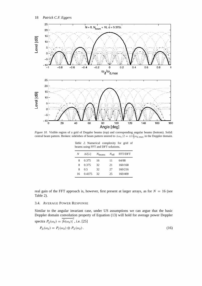
As the DFT approach can be tailor-made only to provide beams within the desired sector,the DFT complexity should be taken asN · Neff when comparing with the FFT approach.Table 2 shows DFT and FFT numerical complexities for different array and grid setups. FortheNbeams= 16 and anti-alias sampling grid of Figure 10, Table 2 presents 27% numericalsavings using the FFT. This, however, drops to 5% when the grid increases toNbeams= 32.When Nyquist sampling is used in the array instead(1l = 0.5λ as in TSUNAMI II [9]), Neff

will be larger and consequently the FFT will again perform better (26%) than the DFT. The


Figure 10. Visible region of a grid of Doppler beams (top) and corresponding angular beams (bottom). Solid:central beam pattern. Broken: sidelobes of beam pattern steered to±ωs/2= ±11

3ωd,max in the Doppler domain.

Table 2. Numerical complexity for grid ofbeams using FFT and DFT solutions.

N 1l[λ] Nbeams Neff FFT/DFT

8 0.375 16 11 64/88

8 0.375 32 21 160/168

8 0.5 32 27 160/216

16 0.4375 32 25 160/400

real gain of the FFT approach is, however, first present at larger arrays, as forN = 16 (seeTable 2).

3.4. AVERAGE POWER RESPONSE

Similar to the angular invariant case, under US assumptions we can argue that the basicDoppler domain convolution property of Equation (13) will hold for average power Doppler

spectraPh(ωd) = |h(ωd)|2, i.e. [25]

Pm(ωd) = Pv(ωd)⊗ Pw(ωd) . (16)


3.5. CORRELATION FUNCTIONS

Correlation functions in the BS Doppler and BS spatial domain can be adopted from the MSdescriptions found in the classical literature [1, 2, 31]. The only difference in the case of alinear array is the separation of elements and the array effects.

The BS spatial and BS Doppler cross-correlations follow Equation (16) assuming WSS,just using cross-power spectra instead (between two different Doppler beams from two arrays)

Pm12(ωd) = m1(ωd) · m∗2(ωd)⇔ Rm12(l) =∫L

m1(η) ·m∗2(η − l)dη= Rv12(l) · Rw12(l)

M12(l) = m1(l) ·m∗2(l)⇔ Rm12(ωd) =∫ ωd,max

−ωd,max

m1(ω) · m∗2(ω − ωd)df

= Rv12(ωd)⊗ Rw12(ωd) .

(17)

The auto-correlation functions follow ifm1 = m2. The spatial coherence length is foundfrom ρm(l) and describes the element spacing necessary to achieve decorrelated port out-puts (standard diversity criterion). The Doppler coherence beamwidth represents necessaryDoppler beam separation for decorrelated outputs, analogous to angle diversity in the angularrepresentation.

4. Angular Channel Dispersion

This section addresses issues regarding classification and experimental characterisation ofangular channels. The discussion is focussed on the application of single antenna (or beam)measurements.

4.1. DISPERSIONMETRICS

The varianceσ 2r = E[r2] − E[r]2 of the domain variabler is an often used measure of

dispersion. This measure is straightforward and well applied in the temporal domain and inthe Doppler domains. However, low sampling frequencies often exist in the case of the BSvirtual Doppler domain, due to element spacings close to1l = λ/2 in the antenna arrays. Thiscan result in wraparound aliasing (circular convolution aroundωs/2) such that the expectationvalues are not well defined. The angular spread has been used in modelling [7] and in mea-surements [12, 14]. This assumes, however, very compact pdfs so that a Cartesian unwrappingof the cyclic angular distribution follows [12, 14]. The mean angle can be estimated by thecentre of gravity approach [12, 14], which is unambiguous with respect to the cyclicity of theangular domain.

Note that traditional antenna parameters such as beamwidths (which are level crossingbased) are not suitable to describe environment responses due to their often erratic shape,thus being difficult to apply unambiguously. Nor is the directivityD = 4π · Umax/Prad [24,28] well suited for describing the environment spreading (Umax is the maximum radiationintensity [W/unit solid angle] andPrad [W] is the total radiated power in all directions due tothe environment response). Consequently, asPrad is integrated over the angular domain, anyinformation about compact or wide angular distributions is lost.


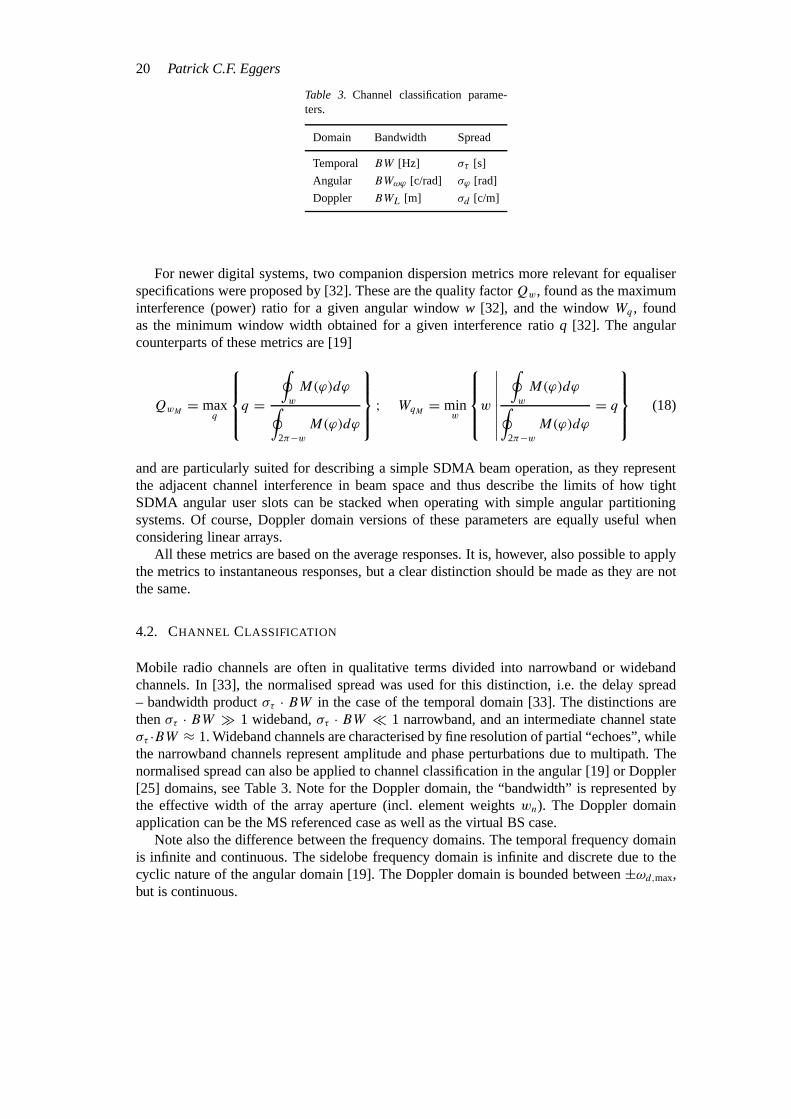
Table 3. Channel classification parame-ters.

Domain Bandwidth Spread

Temporal BW [Hz] στ [s]

Angular BWωϕ [c/rad] σϕ [rad]

Doppler BWL [m] σd [c/m]

For newer digital systems, two companion dispersion metrics more relevant for equaliserspecifications were proposed by [32]. These are the quality factorQw, found as the maximuminterference (power) ratio for a given angular windoww [32], and the windowWq , foundas the minimum window width obtained for a given interference ratioq [32]. The angularcounterparts of these metrics are [19]

QwM = maxq

q =∮w

M(ϕ)dϕ∮2π−w

M(ϕ)dϕ

; WqM = minw

w∣∣∣∣∣∣∣∣∮w

M(ϕ)dϕ∮2π−w

M(ϕ)dϕ

= q

(18)

and are particularly suited for describing a simple SDMA beam operation, as they representthe adjacent channel interference in beam space and thus describe the limits of how tightSDMA angular user slots can be stacked when operating with simple angular partitioningsystems. Of course, Doppler domain versions of these parameters are equally useful whenconsidering linear arrays.

All these metrics are based on the average responses. It is, however, also possible to applythe metrics to instantaneous responses, but a clear distinction should be made as they are notthe same.

4.2. CHANNEL CLASSIFICATION

Mobile radio channels are often in qualitative terms divided into narrowband or widebandchannels. In [33], the normalised spread was used for this distinction, i.e. the delay spread– bandwidth productστ · BW in the case of the temporal domain [33]. The distinctions arethenστ · BW � 1 wideband,στ · BW � 1 narrowband, and an intermediate channel stateστ ·BW ≈ 1. Wideband channels are characterised by fine resolution of partial “echoes”, whilethe narrowband channels represent amplitude and phase perturbations due to multipath. Thenormalised spread can also be applied to channel classification in the angular [19] or Doppler[25] domains, see Table 3. Note for the Doppler domain, the “bandwidth” is represented bythe effective width of the array aperture (incl. element weightswn). The Doppler domainapplication can be the MS referenced case as well as the virtual BS case.

Note also the difference between the frequency domains. The temporal frequency domainis infinite and continuous. The sidelobe frequency domain is infinite and discrete due to thecyclic nature of the angular domain [19]. The Doppler domain is bounded between±ωd,max,but is continuous.


4.3. EXPERIMENTS

Experiments on BS angular conditions have mainly been of the indirect type, i.e. disclosingbranch decorrelation properties of space diversity systems, thereby representing the spatialauto-correlation function at the BS [2, 8]. Now, new measurement considerations appear usingdirect angular sounding, which will be discussed in this section.

4.3.1. Measurement TechniquesWhen performing angular sounding at the BS, we can distinguish between

• Rotating antenna/beam vs. super resolution algorithms (the latter requires multiple ele-ments and post-processing or extremely fast DSPs).

• Angular invariant vs. angular variant (electronically scanned beams), i.e. circular (ormechanically rotated antenna) vs. linear arrays.

• Real arrays vs. virtual arrays (the latter is less complex hardware-wise, but requires nearstatic channel conditions and post-processing).

• Instantaneous vs. average responses (the first requires real time multi-element recordingin dynamic channel conditions and is very complex hardware wise [30]).

Direct angular sounding at the BS first seems to be reported in [2] for narrowband conditions,where the first wideband sounding seems to be due to TSUNAMI [12] and includes polari-sation discrimination. We will concentrate here on beam-oriented sounding. Super resolutionalgorithms applied to instantaneous responses are found in [17].

4.3.2. Measurement Enhancement Techniques

Angular inverse Wiener filtering for sidelobe suppressionIn the temporal domain, Wiener filtering can be used to compensate measurements for theundesired influence of the measurement system [34]. However, for angular invariant condi-tions, the angular relation in Equation (1) constitutes similar frequency domain properties(multiplication, see Equation (2)) as the convolution in the temporal domain. Thus, inverseWiener filtering can be applied in the angular domain as well to suppress the influence of themeasuring antenna sidelobes.

Inverse Wiener filtering applied to the deconvolution of a perceived environment patternestimatee(ϕω) = m(ϕω) · wWiener(ϕω) was first introduced by [12, 14]. An extended Wienerfilter as the one in [34] was used

wWiener(ωϕ) = a(−ωϕ) · wshaping(ωϕ)

|a(−ωϕ)|2+ γ · NSR(ωϕ). (19)

NSR is the noise to signal ratio|N |2/|e|2 andγ is a scalar<1, chosen to underestimate thenoise [34]. A compensating windowwshapingis applied to shape an effective antenna patternto a known sidelobe level and control the effect of excessive noise influence [12, 34].

This procedure can be applied both to instantaneous and to average responses [12], pro-vided US conditions apply, i.e. Equation (3). However, there is no advantage in applying thistechnique in the BS Doppler domain, as only the array weighting functionw(l) influence willbe affected [25] and which we already fully control.


Table 4. WSSUS channel moments.

Domain Variance Mean

Temporal σ2τe = σ2

τm − σ2τh τe = τm = τh

Angular σ2ϕe = σ2

ϕm − σ2ϕa ϕe = ϕm + ϕa

Doppler σ2dv= σ2

dm− σ2

dwfdv = fdm − fdw

The application of this processing technique in the invariant angular domain was laterintroduced to and adopted by [35] and [36], via COST2312 and personal contacts.

Dispersion compensation by variance subtractionUnder temporal wideband conditions, [37] found a variance subtraction property for the delayspreadστ (see Table 4). This effectively compensates the influence of the measuring systemsh(τ), from the measurementmτ(τ), to produce a high-resolution estimate of the varianceσ 2

τe

of the environmenteτ (τ ).However, in US narrowband conditions, the noncoherent voltage summation resulting in

the average power relation of Equation (3) yields a similar relation for the angular spread [12,18] (see Table 4). The correlation property in Equation (3) results in an addition property inthe angular domain for the odd order moments [18].

Similarly, from Equation (16), we obtain a variance subtraction property for the Dopplerspread in the case of linear arrays under US channel conditions and high aliasing suppression[25] (see Table 4). The property can also be applied to the MS referenced Doppler domain.However, in this case the spatial sampling frequency is often so high (windowing influencelow), that little is gained from this operation.

Note thatσdv andfdv are estimates compensated for the array windowing (AF) influenceand are still subject to the weighting due to the antenna elementg(fd). We can callσdv andfdvthe effective Doppler spread and mean, while the true environment Doppler spread and meanareσd andfde. However, if the element pattern is a constant over the illuminating environmentregion, i.e.g(ϕ) = constant|e(ϕ)<>0, then effective and actual environment spreads and meansare identical, i.e.σdv = σde andfdv = fde. The array window Doppler spread and mean areσdw andfdw.

If we define super resolution as a procedure which yields increased resolution beyond whatthe measurement system readily provides, then the variance subtractions of Table 4 providestatistical super resolutions of the channel spreadsσ .

The spreading measure of the total angular direction of arrival (DOA) distribution is rel-evant when establishing angular auto-correlation functions as Equation (5). However, whendesigning DOA models, the spreading measures can also be applied to characterise partialDOA clusters. This would be analogous to the COST207 hilly terrain power delay profile(PDP) being composed of two clusters with a given separation and individual spread [38–41].

2 European research programme in the field of “Evolution of Land Mobile (including cordless) RadioCommunications”.


4.4. EFFECTIVE ANTENNA PARAM ETERS

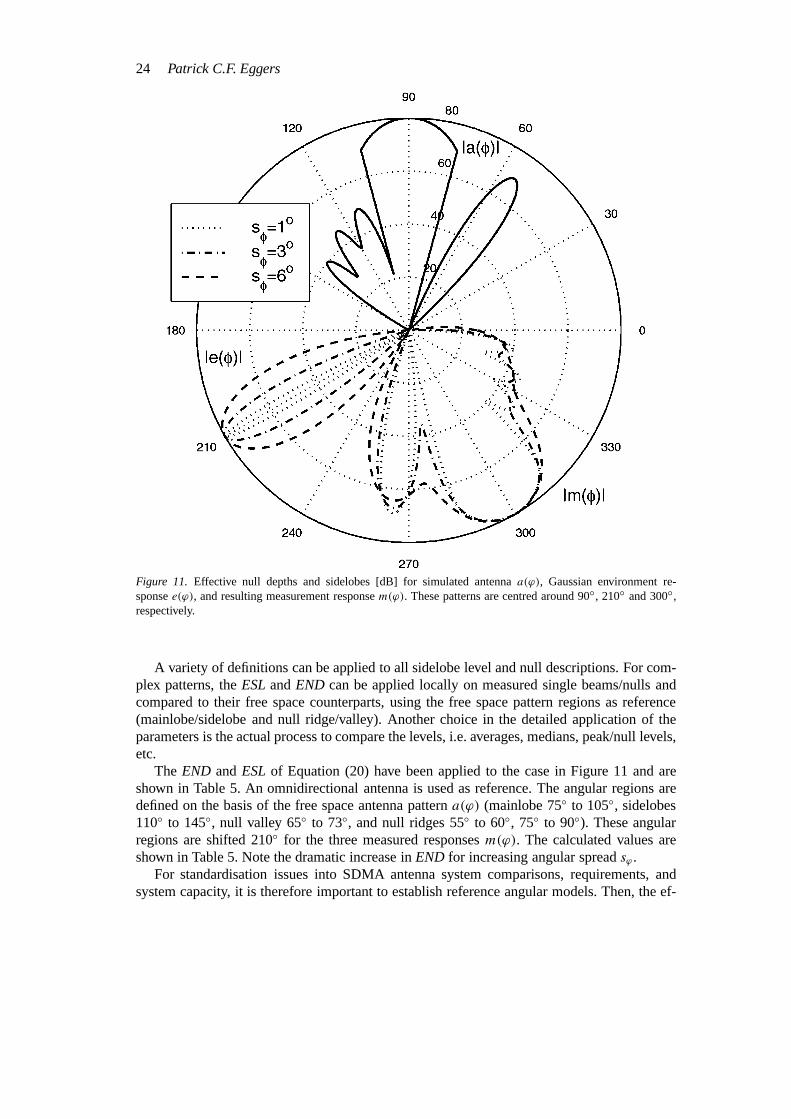
Antenna parameters are used for establishing design criteria and evaluating existing antennadesigns. Traditional parameters as gain, beamwidth, sidelobe level, and XPD are defined onthe basis of a point source illumination in the far field [24]. In Mobile radio, we rarely havepoint source conditions. In the MS case, [42] defined mean effective gain (MEG) as a relevantdescriptor of the perceived gain in cluttered environments. However, at the BS we would liketo know how good an antenna is in a beam-focussing or nulling situation. Here, the free spaceparameters fail as they do not include the environments. In Figure 11, it can be seen howthe angular scattering of the environment fills in the nulls and raises the sidelobe level of theperceived patternm(ϕ). It can also be seen howm(ϕ) appears to be shifted 300◦, due to thesum of the individual shiftsa(ϕ) 90◦ ande(ϕ) 210◦, as discussed in Section 2.1.

Consequently, there is no point in assuming a free space pattern with extreme free spacenull depths or sidelobe suppression when performing beam-operated SDMA capacity analysis,as the environment will “fill-in” the response due to the correlation relation of Equation (1).The use of free space patterns with point source hypothesis leads to over-optimistic capacityresults.

Thus, effective antenna parameters have to be used when specifying an antenna system.Such parameters cater to the influence of the environment, as the angular spreading of theenvironment set limits to aim for in the worthwhile angular selectivity and free space patternpurity (beam widths, null depth). This sets natural limits on worthwhile hardware require-ments, i.e. ADC resolution, amplifier linearity, etc. This is contrary to, for example, spaceapplications involving satellites where the free space pattern is well applied in link qualitydescriptions.

In principle, traditional antenna parameter definitions could be used if based on the mea-surement responsem(ϕ) instead of the free space antenna patterna(ϕ). However, to avoidambiguities, level crossing parameters should be avoided and power integration or quantiledistribution parameters used instead. [12] and [14] defined an effective antenna parameter tobe used in the BS case, namely the effective sidelobe level(ESL)of a test antenna

ESLtest=med

(M(ϕ)test

M(ϕ)reference

)mainlobe

med

(M(ϕ)test

M(ϕ)reference

)sidelobes

; ENDtest=med

(M(ϕ)test

M(ϕ)reference

)null valley

med

(M(ϕ)test

M(ϕ)reference

)null ridge

(20)

based on medians. Note that this parameter definition is relative to the response of a widebeamsector reference antenna. The reference antenna response acts as an estimator of the overallpath loss, including log-normal fading [12, 14]. This is so that the measurement can be per-formed with a static antenna orientation, while letting the MS probe the environment undermovement. With this normalisation, theESLcan operate under nonstationary measurementconditions. TheESLcan provide a picture of angular-slot power spillover and therefore doesrepresent simple SDMA adjacent angular slot interference for a given antenna in a givenenvironment. Also shown in Equation (20) is a similar definition of an effective null depth(END).

More sophisticated algorithms that also include an estimate of the angular spreading ofeach interferer component may be designed in such a way that nulls are created wide enoughto “absorb” all interferer power. In such a case, theEND or ESLof the measurement will notdeviate dramatically from the free space case.


Figure 11. Effective null depths and sidelobes [dB] for simulated antennaa(ϕ), Gaussian environment re-sponsee(ϕ), and resulting measurement responsem(ϕ). These patterns are centred around 90◦, 210◦ and 300◦,respectively.

A variety of definitions can be applied to all sidelobe level and null descriptions. For com-plex patterns, theESLandEND can be applied locally on measured single beams/nulls andcompared to their free space counterparts, using the free space pattern regions as reference(mainlobe/sidelobe and null ridge/valley). Another choice in the detailed application of theparameters is the actual process to compare the levels, i.e. averages, medians, peak/null levels,etc.

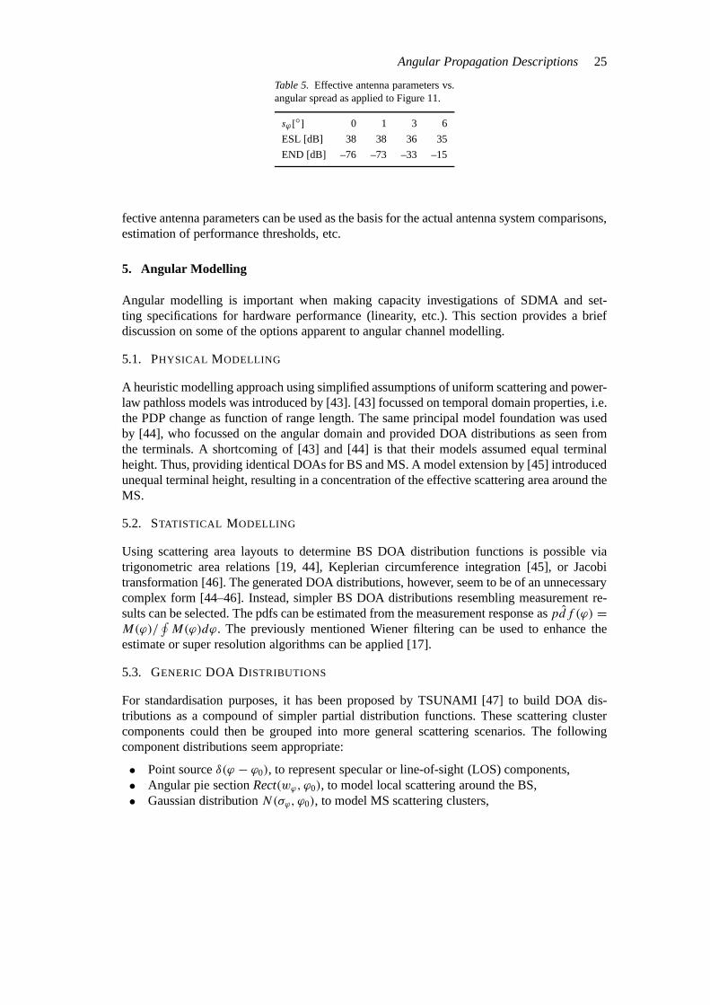
The END andESLof Equation (20) have been applied to the case in Figure 11 and areshown in Table 5. An omnidirectional antenna is used as reference. The angular regions aredefined on the basis of the free space antenna patterna(ϕ) (mainlobe 75◦ to 105◦, sidelobes110◦ to 145◦, null valley 65◦ to 73◦, and null ridges 55◦ to 60◦, 75◦ to 90◦). These angularregions are shifted 210◦ for the three measured responsesm(ϕ). The calculated values areshown in Table 5. Note the dramatic increase inEND for increasing angular spreadsϕ .

For standardisation issues into SDMA antenna system comparisons, requirements, andsystem capacity, it is therefore important to establish reference angular models. Then, the ef-


Table 5. Effective antenna parameters vs.angular spread as applied to Figure 11.

sϕ [◦] 0 1 3 6

ESL [dB] 38 38 36 35

END [dB] –76 –73 –33 –15

fective antenna parameters can be used as the basis for the actual antenna system comparisons,estimation of performance thresholds, etc.

5. Angular Modelling

Angular modelling is important when making capacity investigations of SDMA and set-ting specifications for hardware performance (linearity, etc.). This section provides a briefdiscussion on some of the options apparent to angular channel modelling.

5.1. PHYSICAL MODELLING

A heuristic modelling approach using simplified assumptions of uniform scattering and power-law pathloss models was introduced by [43]. [43] focussed on temporal domain properties, i.e.the PDP change as function of range length. The same principal model foundation was usedby [44], who focussed on the angular domain and provided DOA distributions as seen fromthe terminals. A shortcoming of [43] and [44] is that their models assumed equal terminalheight. Thus, providing identical DOAs for BS and MS. A model extension by [45] introducedunequal terminal height, resulting in a concentration of the effective scattering area around theMS.

5.2. STATISTICAL MODELLING

Using scattering area layouts to determine BS DOA distribution functions is possible viatrigonometric area relations [19, 44], Keplerian circumference integration [45], or Jacobitransformation [46]. The generated DOA distributions, however, seem to be of an unnecessarycomplex form [44–46]. Instead, simpler BS DOA distributions resembling measurement re-sults can be selected. The pdfs can be estimated from the measurement response aspdf (ϕ) =M(ϕ)/

∮M(ϕ)dϕ. The previously mentioned Wiener filtering can be used to enhance the

estimate or super resolution algorithms can be applied [17].

5.3. GENERIC DOA DISTRIBUTIONS

For standardisation purposes, it has been proposed by TSUNAMI [47] to build DOA dis-tributions as a compound of simpler partial distribution functions. These scattering clustercomponents could then be grouped into more general scattering scenarios. The followingcomponent distributions seem appropriate:

• Point sourceδ(ϕ − ϕ0), to represent specular or line-of-sight (LOS) components,• Angular pie sectionRect(wϕ, ϕ0), to model local scattering around the BS,• Gaussian distributionN(σϕ, ϕ0), to model MS scattering clusters,


• Laplacian distributionL(σϕ, ϕ0), to model to model MS scattering clusters,

where the first three stem from [47] (the Gaussian though being a classical suggestion [7]).The Laplacian distribution seems to provide good fits to angular measurements performedby TSUNAMI II [48]. A similar approach has been taken by [40] and [41]; however, hereusing generic scattering area layouts to build a full model, together with assumption of thetransfer process from the MS to BS (i.e. single bouncing). This approach readily yields tem-poral/spatial relations, but is difficult to handle in closed form expressions just as the otherphysical models.

There are also indications that the statistical distributions in the temporal and the angulardomains are similar but uncorrelated between polarisations [23], for nonline-of-sight (NLOS)situations, i.e. the PDP and the spatial decorrelation are of similar shape and value. Thus, forsimplicity we can model the polarisations with identical distributions but with independentoutcome.

Furthermore, there are indications that the angular and temporal domains can be modelledindependently [17], i.e.pdf(ϕ, τ) = pdf(ϕ) · pdf(τ ). This makes the construction of a purestatistical model easier to fit experimental knowledge, while avoiding the need to resort togeometric/physical layouts as in [40] and [41]. For the temporal domain, the exponential decayfunction has found widespread use, for example, standardised in COST207 [38].

The advantage of statistical over physical modelling is simplicity, which can be utilisedfor increased speed in system simulations and possible closed form solutions that displayparameter dependencies.

6. Conclusions

The following important issues have been identified with regard to angular propagation rele-vant for beam-oriented adaptive antennas and SDMA.

6.1. ANGULAR INVARIANT ANTENNA SYSTEMS

• Measurement processing using inverse Wiener filtering to suppress sidelobe effects andvariance subtraction to suppress the influence of the antennas on the angular spread.These applications were introduced by [12] and [14].

• Angular correlation function descriptions providing means for estimating dynamic multi-beam diversity potentials, i.e. when two or more beam formers/antenna systems areapplied to a single user.

• Effective antenna parameters should be used (instead of free space pattern parameters)with reference to the environment. This may ease hardware requirements on the antennasystem, but require standardised angular environment models for comparisons.

6.2. LINEAR AND PLANAR ARRAYS

• The virtual BS Doppler domain provides beam orientation invariance.• For beam steering, acquisition, and tracking, this paper has proposed the BS Doppler

domain for the generation of a fan of beams. The Doppler domain beams provide fasteralgorithms via straight FFTs than via direct angular beam DFTs (26% less computingeffort for an 8 element array with a total of 32 Doppler beams).


• The statistics of the signal along the arrays elements are known [27], i.e., narrowbandfading levels, level crossing rate, phase gradients, etc.

References

1. R.H. Clarke, “A Statistical Theory of Mobile-Radio Reception”,Bell Syst. Techn. J.pp. 957–999, 1968.2. W.C. Jakes Jr., (ed.),Microwave Mobile Communications, IEEE Press: Piscataway, NJ, U.S.A., 1993.3. W.C.-Y. Lee, “Finding the Approximate Angular Probability Density Function of Wave Arrival by Using a

Directional Antenna”,IEEE Trans. Ant. Prop., Vol. AP-21, No. 3, pp. 328–334, 1973.4. F. Ikegami and S. Yoshida, “Analysis of Multipath Propagation Structure in Urban Mobile Radio Environ-

ments”,IEEE Trans. Ant. And Prop., Vol. AP-28, No. 4, pp. 531–537, 1980.5. J. Fuhl, J.-P. Rossi and E. Bonek, “High-Resolution 3-D Direction-of-Arrival Determination for Urban

Mobile Radio”,IEEE Trans. Ant. & Prop., Vol. 45, No. 4, pp. 672–682, 1997.6. A.M.D. Turkmani and J.D. Parsons, “Characterisation of Mobile Radio Signals: Model Description” and

“Characterisation of Mobile Radio Signals: Base Station Crosscorrelation”,IEE Proc.-I, Vol. 138, No. 6, pp.549–556 and pp. 557–565, 1991.

7. F. Adachi, M.T. Feeney, A.G. Williamson and J.D. Parsons, “Crosscorrelation Between the Envelopes of 900MHz Signals Received at a Mobile Radio Base Station Site”,IEE Proc., Vol. 133, Pt. F., No. 6, pp. 506–512,1986.

8. W.C.-Y. Lee, “Effects on Correlation Between Two Mobile Radio Base-Station Antennas”,IEEE Trans. onCom., Vol. COM-21, No. 11, pp. 1214–1223, 1973.

9. P.E. Mogensen, P. Zetterberg, H. Dam, P. Leth-Espensen and F. Fredriksen, “Algorithms and Antenna Ar-ray Recommendations (Part 1)”, ACTS TSUNAMI II deliverable AC020/AUC/A1.2/DR/P/005/b1, 15 May1997.

10. M. Barret and P. Eggers, “TSUNAMI Project Seminar”, RACE II TSUNAMI project reportR2108/ERA/WP1-3/DS/P/1021/b1, Dec. 1995.

11. J. Wigard, “Optimum Combining in DECT”, M.Sc.E.E. thesis, Aalborg University Denmark, Jan. 1995.12. P.C.F. Eggers, G.F. Pedersen and K. Olesen, “Multi Sensor Propagation”, RACE II TSUNAMI deliverable,

R2108/AUC/WP3.1/DS/I/046/b1, Aug. 17, 1994.13. P.C.F. Eggers, “Einfluß der Geländestreuung auf die Strahlungseigenschaften von Basisstationsrichtantennen

für Mobilfunksysteme”,(NE) Nachrichtentechnik-Elektronik, No. 4, pp. 57–62, 1995 (in German).14. P.C.F. Eggers, “Angular Dispersive Mobile Radio Environments Sensed by Highly Directive Base Station

Antennas”,Proc. of PIMRC’95, Toronto Canada, Sep. 27–29 1995, pp. 522–526.15. P. Leth-Espensen, P. Zetterberg, P.E. Mogensen F. Frederiksen, K. Olesen and S. Leth Larsen, “Algo-

rithm Test Using Measurements From an Adaptive Antenna Array Testbed for GSM/UMTS”,Proc. IEEEPIMRC’97, Helsinki Finland, Sep. 1–4 1997, pp. 155–159.

16. U. Martin, “Spatio-temporal Radio Channel Characteristics in Urban Macrocells”,IEE Proc.-Radar, SonarNavig., Vol. 145, No. 1, pp. 42–49, 1998.

17. K.I. Pedersen, P.E. Mogensen, B.F. Fleury, F. Fredriksen, K. Olesen and S.L. Larsen, “Analysis of Time,Azimuth and Doppler Dispersion in Outdoor Radio Channels”,Proc. ACTS Mob. Com. Summit ’97, Aalborg,Denmark, 7–10 Oct. 1997, pp. 308–313.

18. P.C.F. Eggers, “Quantitative Descriptions of Radio Environment Spreading Relevant to Adaptive AntennaArrays”, Proc. of EPMCC’95, Bologna, Italy, 28–30 Nov. 1995, pp. 68–73.

19. P.C.F. Eggers, “Angular – Temporal Domain Analogies of the Short-term Mobile Radio Propagation Channelat the Base Station”,Proc. IEEE PIMRC’96, Taipei, Taiwan, Oct. 15–18 1996, pp. 742–746.

20. R.G. Vaughan and J. Bach Andersen, “Antenna Diversity in Mobile Communications”,IEEE Trans. Veh.Techn., Vol. VT-36, pp. 149–172, 1987.

21. R.G. Vaughan, “Pattern Rotation and Translation in Uncorrelated Source Distributions for Multiple BeamAntenna Design”,Proc. of PIERS, Vol. 2, Hongkong, Jan. 1997, p. 357.

22. R.G. Vaughan, “Pattern Rotation and Translation in Uncorrelated Source Distributions for Multiple BeamAntenna Design”, accepted byIEEE Trans. on Ant. & Prop.(submitted Oct. 1996).

23. P.C.F. Eggers, J. Toftgård and A.M. Oprea, “Antenna Systems for Base Station Diversity in Urban Small andMicro Cells”, IEEE J-SAC, Vol. 11, No. 7, pp. 1046–1057, 1993.

24. C.A. Balanis,Antenna Theory – Analysis and Design, John Wiley & Sons: U.S.A., 1982.


25. P.C.F. Eggers, “Super Resolution and Deconvolution of Angular Power Spectra”,Proc. IEEE PIMRC’97,Helsinki, Finland, Sep. 1–4 1997, pp. 801–805.

26. P. Petrus, J.H. Reed and T.S. Rappaport, “Geometrically Based Statistical Channel Model for MacrocellularMobile Environments”,Proc. IEEE Globecom’96, London, U.K., 18–20 Nov. 1996, pp. 1197–1201.

27. J. Bach Andersen, “A Parametric View of Adaptive Antennas in a Scattering Environment”, URSICommSphere Workshop, Lausanne, Switzerland, Feb. 11–14 1997.

28. O. Nørklit, “Jitter Diversity in Multipath Environments”,Proc. IEEE VTC’95, Chicago, Il, U.S.A., July25–28 1995, pp. 853–857.

29. A.V. Oppenheim and R.W. Schafer,Digital Signal Processing, Prentice-Hall: Englewood Cliffs, NJ, U.S.A.,1975.

30. P.E. Mogensen, K.I. Pedersen, P.L.-Espensen, B. Fleury, F. Fredriksen, K. Olesen and S.L. Larsen, “Prelime-nary Measurement Results From an Adaptive Antenna Array Testbed for GSM/UMTS”,Proc. of VTC’97,Phoenix Az., U.S.A., May 5–7 1997.

31. W.C.-Y Lee,Mobile Communications Engineering, McGraw-Hill: U.S.A., 1972.32. J.-P. de Weck and J. Ruprecht, “Real-time ML Estimation of Very Frequency Selective Multipath Channels”,

Proc. IEEE Globecom, San Diego, CA, U.S.A., 1990, pp. 908.5.1-6.33. J. Bach Andersen, P. Eggers and B.L. Andersen, “Propagation Aspects of Datacommunication Over the

Radio Channel – A Tutorial”,Proc. EUROCON’88, Stockholm, Sweden, June 13–17 1988, pp. 301–305.34. A.J. Levy, J.-P. Rossi, J.-P. Barbot and J. Martin, “An Improved Sounding Technique Applied to Wideband

Mobile 900 MHZ Propagation Measurements”,Proc. IEEE VTC’90, Orlando, Fl, U.S.A., May 6–9 1990,pp. 513–519.

35. A. Klein, W. Mohr, R. Thomas, P. Weber and B. Wirth, “Direction-of-Arrival of Partial Waves in WidebandMobile Radio Channels for Intelligent Antenna Concepts”,Proc. of IEEE VTC’96, Atlanta, GA, U.S.A.,April 28–May 1 1996.

36. J. Laiho-Steffens, “Two-dimensional Characterisation of the Mobile Propagation Environment”, Ph.D.Thesis, Helsinki Univ. of Techn., Finland, 3/6 1996.

37. A.A.M. Saleh and R.A. Valenzuela, “A Statistical Model for Indoor Multipath Propagation”,IEEE J. Select.Areas Com., Vol. 5, No. 2, pp. 128–137, 1987.

38. COST207,Digital Land Mobile Radio, Final Report, EU: Luxemburg, 1989.39. U. Martin, “Statistical Mobile Radio Channel Simulator for Multiple-Antenna Reception”,Proc. IEICE Int.

Symp. on Antennas, Sep. 1996.40. J. Fuhl, A.F. Molish and E. Bonek, “Unified Channel Model for Mobile Radio Systems with Smart

Antennas”,IEE Proc.-Radar, Sonar Navig., Vol. 145, No. 1, pp. 32–41, 1998.41. J.J. Blanz and P. Jung, “A Flexibly Configurable Spatial Model for Mobile Radio Channels”,IEEE Trans. on

Com., Vol. 46, No. 3, pp. 367–371, 1998.42. J. Bach Andersen and F. Hansen, “Antennas for VHF/UHF Personal Radio”,IEEE Trans. Veh. Techn.,

Vol. VT-26, No. 4, pp. 349–357, 1977.43. J. Bach Andersen and P.C.F. Eggers, “A Heuristic Model of Power Delay Profiles in Landmobile Com-

munications”,Proc. 1992 URSI Int. Symp. on EM Theory, Sydney, Australia, Aug. 17–20, 1992, pp.55–57.

44. J.C. Liberti and T.S. Rappaport, “A Geometrically Based Model for Line-of-sight Multipath RadioChannels”,Proc. IEEE VTC’96, Atlanta, GA, U.S.A., April 28–May 1 1996, pp. 844–848.

45. O. Nørklit and J. Bach Andersen, “Diffuse Channel Model and Experimental Results for Array Antennasin Mobile Environments”, to be published inIEEE Trans on Ant. and Prop., special issue on WirelessCommunications, June 1998.

46. P.C.F. Eggers, “Generation of Base Station DOA Distributions via Jacobi Transformation of ScatteringAreas”,Elec. Letters, Vol. 34, No. 1, pp. 24–26, 1998.

47. P.C.F. Eggers, “Directional Propagation Characterisation”, RACE II TSUNAMI I reportR2108/AUC/WP1.2/DN/P/054/a1. Input to STG2.4 and ETSI SMG5.

48. K.I. Pedersen, P.E. Mogensen and B.F. Fleury, “Power Azimuth Spectrum in Outdoor Environments”,Elec.Let., Vol. 33, No. 18, pp. 1583–1584, 1997.


Patrick C.F. Eggers was born in Stockholm, Sweden, in 1957. He received an M.Sc.E.E.degree from Aalborg University, Aalborg, Denmark, in 1984. He has been employed at Aal-borg University since 1984, mainly as a full-time researcher in mobile radio communications.His current position is research professor at the Center for PersonKommunikation, AalborgUniversity. He has been an active participant in the COST207 and COST231 working groupson propagation in the same period and is now participating in the follow-up project COST259.He is a chapter editor of the final report of COST231. He worked in Wellington, New Zealand,from October 1988 to November 1989 for Telecom New Zealand. He was responsible for theangular propagation work performed under the RACE II project, TSUNAMI. He is one ofthe initiators of the recently established, English-taught, international M.Sc.E.E. course atAalborg University specializing in mobile radio communications. His main interest lies in thefield of propagation and mobile communications.

Documents

Angular Propagation Descriptions Relevant for Base Station Adaptive Antenna …kom.aau.dk/~pe/education/phd/litt/kluwer1999.pdf · 2004-07-21 · changes in the partial selection