Embed Size (px)
Citation preview
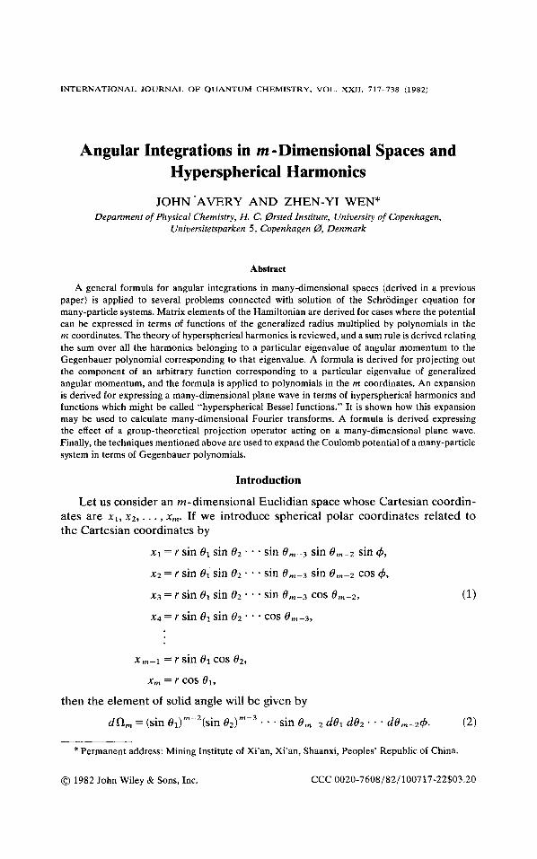
INTERNATIONAL JOURNAL OF QUANTUM CHEMISTRY, VOL. XXII, 717-738 (1982)
Angular Integrations in m -Dimensional Spaces and Hyperspherical Harmonics
JOHN ‘AVERY AND ZHEN-YI WEN* Department of Physical Chemistry, H. C. 0rsted Institute, University of Copenhagen,
Universitetsparken 5 , Copenhagen 0, Denmark
Abstract
A general formula for angular integrations in many-dimensional spaces (derived in a previous paper) is applied to several problems connected with solution of the Schrodinger equation for many-particle systems. Matrix elements of the Hamiltonian are derived for cases where the potential can be expressed in terms of functions of the generalized radius multiplied by polynomials in the m coordinates. The theory of hyperspherical harmonics is reviewed, and a sum rule is derived relating the sum over all the harmonics belonging to a particular eigenvalue of angular momentum to the Gegenbauer polynomial corresponding to that eigenvalue. A formula is derived for projecting out the component of an arbitrary function corresponding to a particular eigenvalue of generalized angular momentum, and the formula is applied to polynomials in the m coordinates. An expansion is derived for expressing a many-dimensional plane wave in terms of hyperspherical harmonics and functions which might be called “hyperspherical Bessel functions.” It is shown how this expansion may be used to calculate many-dimensional Fourier transforms. A formula is derived expressing the effect of a group-theoretical projection operator acting on a many-dimensional plane wave. Finally, the techniques mentioned above are used to expand the Coulomb potential of a many-particle system in terms of Gegenbauer polynomials.
Introduction
Let us consider an rn-dimensional Euclidian space whose Cartesian coordin- ates are xl, x2, . . . , x,. If we introduce spherical polar coordinates related to the Cartesian coordinates by
x1 = r sin O1 sin O2 . * * sin sin OmP2 sin 9, x 2 = r sin O1 sin 02 * - * sin O m P 3 sin
x 3 = r sin O1 sin 02 - * * sin Om-3 cos O m - 2 ,
x4 = r sin B1 sin O2
cos 9,
cos
x,-1 = r sin O1 cos 02,
x, = r cos 01,
then the element of solid angle will be given by
dR, = (sin B1)m-2(sin 02)m-3 - . sin O m P 2 dol do2 - - - d0,-2q5. (2)
* Permanent address: Mining Institute of Xi’an, Xi’an, Shaanxi, Peoples’ Republic of China.
@ 1982 John Wiley & Sons, Inc. CCC 0020-7608/82/100717-22$03.20
718 AVERY AND WEN
In previous papers [ l , 21 it was shown that if n l , n2, n3, . . . , n, are positive integers or zero, then
r"l"(n) = dn,, x;1xZn2x;3 * * * xkm I N,rn
- ( m + n -2)!! j = l -b. otherwise,
( n j - l ) ! ! , all ni's even, (3)
2 2 2 2 where n = n l + n 2 + - n,, r = X I + x 2 + * . +x, and
m even,
m odd.
For example, in a three-dimensional space with Cartesian coordinates x, y, and 2, we have the angular integration formula
4.rrrt11fn2tn3 ( n l - l)!!(nZ- l)!!(n3- l)!!,
r ( n l + n 2 + n 3 + l)!! n1, n2, and 123 even, otherwise
( 5 )
where
and
n(n -2)(n - 4 ) - 6 * 4 * 2, PI even,
n ( n -2)(n -4) * 7 3 1, n odd, (7) n ! ! =
( - l ) ! ! = 1.
Although Eq. (3) was derived as part of a series of papers related to charge density analysis, we felt that it might prove to be very useful in other contexts, and we have therefore investigated various other applications of the formula. For example, in certain problems, such as the analysis of large-amplitude motions in molecules or the study of nuclear motions in chemical reactions [3-71, it may be possible to express the potential of a many-particle system in the form
where
ANGULAR INTEGRATIONS 719
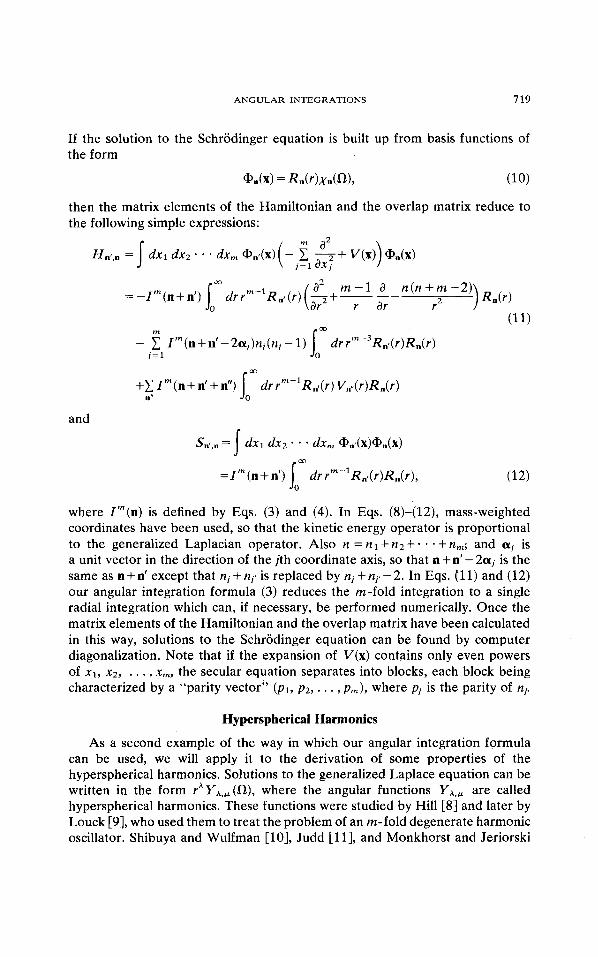
If the solution to the Schrodinger equation is built up from basis functions of the form
= Rdr)Xda), (10)
then the matrix elements of the Hamiltonian and the overlap matrix reduce to the following simple expressions:
+C Im(n+n‘+n”) drrm-lRn,(r)Vn,,(r)Rn(r) n”
and
co
=Im(n+n’) jo drrm -lRn,(r)Rn(r), (12)
where I”(n) is defined by Eqs. (3) and (4). In Eqs. (8)-(12), mass-weighted coordinates have been used, so that the kinetic energy operator is proportional to the generalized Laplacian operator. Also n = n1 + n2 + + n,; and a, is a unit vector in the direction of the jth coordinate axis, so that n +n’ - 2a, is the same as n + n’ except that n, + n,, is replaced by n, + n,, - 2. In Eqs. (1 1) and (12) our angular integration formula (3) reduces the m-fold integration to a single radial integration which can, if necessary, be performed numerically. Once the matrix elements of the Hamiltonian and the overlap matrix have been calculated in this way, solutions to the Schrodinger equation can be found by computer diagonalization. Note that if the expansion of V(x) contains only even powers of xl, x2, . . . , xm, the secular equation separates into blocks, each block being characterized by a “parity vector” ( p l , p 2 , . . . , pm), where p, is the parity of n,.
Hyperspherical Harmonics
As a second example of the way in which our angular integration formula can be used, we will apply it to the derivation of some properties of the hyperspherical harmonics. Solutions to the generalized Laplace equation can be written in the form rhYh,+(Cl), where the angular functions YA+ are called hyperspherical harmonics. These functions were studied by Hill [8] and later by Louck [9], who used them to treat the problem of an rn-fold degenerate harmonic oscillator. Shibuya and Wulfman [lo], Judd [ll], and Monkhorst and Jeriorski
120 AVERY AND WEN
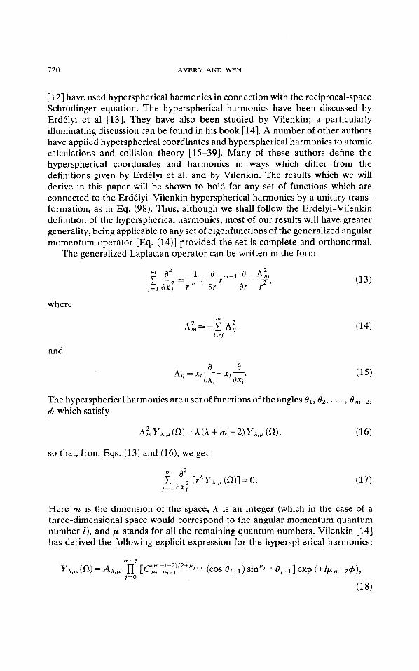
[ 121 have used hyperspherical harmonics in connection with the reciprocal-space Schrodinger equation. The hyperspherical harmonics have been discussed by Erdtlyi et a1 [13]. They have also been studied by Vilenkin; a particularly illuminating discussion can be found in his book [14]. A number of other authors have applied hyperspherical coordinates and hyperspherical harmonics to atomic calculations and collision theory [15-391. Many of these authors define the hyperspherical coordinates and harmonics in ways which differ from the definitions given by Erdtlyi et al. and by Vilenkin. The results which we will derive in this paper will be shown to hold for any set of functions which are connected to the Erdtlyi-Vilenkin hyperspherical harmonics by a unitary trans- formation, as in Eq. (98). Thus, although we shall follow the Erdtlyi-Vilenkin definition of the hyperspherical harmonics, most of our results will have greater generality, being applicable to any set of eigenfunctions of the generalized angular momentum operator [Eq. (14)] provided the set is complete and orthonormal.
The generalized Laplacian operator can be written in the form
where
and
a a A . . = x . - - X j -.
axj axi 11 1
The hyperspherical harmonics are a set of functions of the angles el, 02, which satisfy
A?,, YA,@ (a) = A (A + rn - 2) YA,@ (01,
so that, from Eqs. (13) and (16), we get
Here m is the dimension of the space, A is an integer (which in the case of a three-dimensional space would correspond to the angular momentum quantum number I), and p stands for all the remaining quantum numbers. Vilenkin [14] has derived the following explicit expression for the hyperspherical harmonics:
ANGULAR INTEGRATIONS 72 1
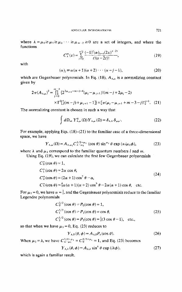
where A = po 2 FI 2 p2
functions * 2 w m - 2 2 0 are a set of integers, and where the
with (a)f = a (a + l)(a + 2) * * (a + j - l), (20)
which are Gegenbauer polynomials. In Eq. (18), A",, is a normalizing constant given by
m - 3
~ T ( A ~ , & ) ~ = {22CL,+lfm-f-4 (PI -/Jf+l ) ! (m -i +2Pf -2) ]=O
xr2[$(m - j ) + ~ , + ~ - l ] } x [ ~ ( p , + p ~ + ~ +m -3-j)!]-'. (21)
The normalizing constant is chosen in such a way that
For example, applying Eqs. (18)-(21) to the familiar case of a three-dimensional space, we have
(cos e) sinF1 8 exp (*ipld), YA+ (~)=AA,,lCA-,l (23) 1/2-fi1
where A and p~ correspond to the familiar quantum numbers I and m. Using Eq. (19), we can calculate the first few Gegenbauer polynomials
c," (cos 0) = 1,
c: (COS e ) = 2a cos e, c; (cos 0) = (2a + 1) cos2 8 -a,
C: (cos 8 ) =*a (a + l)(a + 2) C O S ~ o - 2a (a + 1) cos 0,
(24)
etc.
For pi = 0, we have a = $, and the Gegenbauer polynomials reduce to the familiar Legendre polynomials
(cos 8 ) = Po(c0s 0) = 1,
c : / ~ (COS e ) = pl(cos e ) = cos e, c:" (cos e) = P ~ ( C O S 0) = 3 3 cos o - 11, etc.,
y A , O ( 0 ~ 4 ) = A A , O ~ A (COS e).
(25)
so that when we have ,ul = 0, Eq. (23) reduces to
(26)
(27)
When pl = A, we have Ci!?:rl = CA/2+cL1 = 1, and Eq. (23) becomes
YA,A (0, 4 ) =A"," sin" 6 exp
which is again a familiar result.
722 AVERY AND WEN
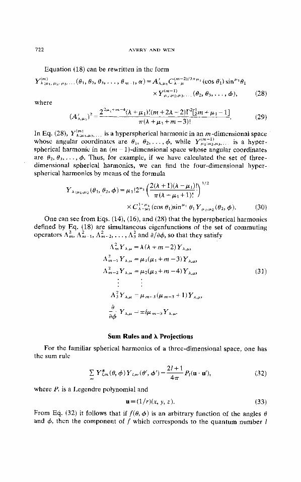
2 2w1 t m - 4 (A + p d ! ( m + 2A - 2)r2[+m + p - 11 (A:,,l)2 = (29) ~ ( h + p l + m -3)!
In Eq. (28), Y~ffl~l, ,z, . . , is a hyperspherical harmonic in an m-dimensional space whose angular coordinates are 01, &,. . . ,4, while YLT.L:),,3 , . . . is a hyper- spherical harmonic in an (m - 1)-dimensional space whose angular coordinates are 02, 0 3 , . . . ,4. Thus, for example, if we have calculated the set of three- dimensional spherical harmonics, we can find the four-dimensional hyper- spherical harmonics by means of the formula
x C~T;; (cos el)sinCL1 o1 Y,,,,, (02, 4). (30)
One can see from Eqs. (14), (16), and (28) that the hyperspherical harmonics defined by Eq. (18) are simultaneous eigenfunctions of the set of commuting operators A;, AkP1, A:-2, . . . , A: and 8/84, so that they satisfy
Sum Rules and X Projections
For the familiar spherical harmonics of a three-dimensional space, one has the sum rule
21+1 C Y T m (034) Y / , m (0’7 4’) = 7 Pl(U * uo, (32) m
where Pf is a Legendre polynomial and
u = (l /r)(x, Y , 2 ) . (33)
From Eq. (32) it follows that if f ( 8 , G ) is an arbitrary function of the angles 8 and 4, then the component of f which corresponds to the quantum number 1
ANGULAR INTEGRATIONS
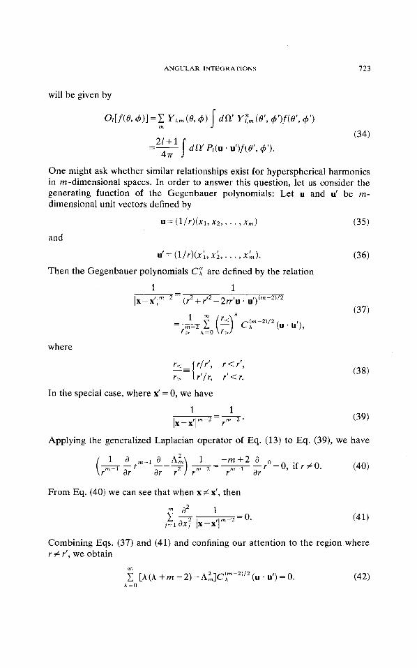
will be given by
723
One might ask whether similar relationships exist for hyperspherical harmonics in m-dimensional spaces. In order to answer this question, let us consider the generating function of the Gegenbauer polynomials: Let u and u’ be m- dimensional unit vectors defined by
u = ( 1 / r ) ( x 1 , X Z , . . . , xrn)
u‘= ( l / r ) ( x i , xb, . . . , x i ) .
(35)
(36)
and
Then the Gegenbauer polynomials CP are defined by the relation
1 - 1 I X - x ’ l m - 2 - (r2+r’2-2rr’u. “ y m - 2
(37) 1 “
(u * u’) 9
where
In the special case, where x‘ = 0, we have
Applying the generalized Laplacian operator of Eq. (13) to Eq. (39) , we have
From Eq. (40) we can see that when x # x’, then
Combining Eqs. (37) and (41) and confining our attention to the region where r # r’, we obtain
m
1 [A (A + m - 2) -hk]Cirn-2)’2 (u - u’) = 0. (42) A =O
124 AVERY AND WEN
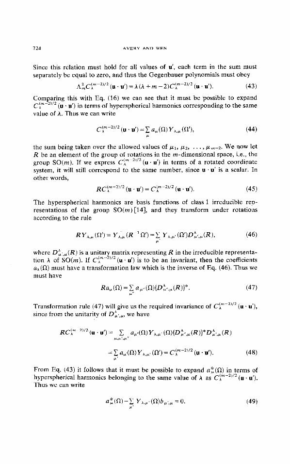
Since this relation must hold for all values of u’, each term in the sum must separately be equal to zero, and thus the Gegenbauer polynomials must obey
hiCimm-2)/2 (U * u’) = A (A + rn - 2)Cimm-2)/2 (U - u’). (43)
Comparing this with Eq. (16) we can see that it must be possible to expand Cj\m--2)’2 (u u’) in terms of hyperspherical harmonics corresponding to the same value of A . Thus we can write
the sum being taken over the allowed values of p l , p2, . . . , pm-2. We now let R be an element of the group of rotations in the rn-dimensional space, i.e., the group SO(rn). If we express Cim-2’/2 (u - u’) in terms of a rotated coordinate system, it will still correspond to the same number, since u - u’ is a scalar. In other words,
RC‘,“-2’/2 (u . u’) = Cim-2) /2(u. u’). (45)
The hyperspherical harmonics are basis functions of class 1 irreducible rep- resentations of the group SO(rn) [14], and they transform under rotations according to the rule
R YA., (n’) = YA;, (R @) = 1 YA.,, (fi’)Dtc,p (R) , (46) ,’
where D^,f,,(R) is a unitary matrix representing R in the irreducible representa- tion A of SO(rn). If CI;”-2’/2(u* u’) is to be an invariant, then the coefficients U A (a) must have a transformation law which is the inverse of Eq. (46). Thus we must have
Transformation rule (47) will give us the required invariance of Cimm-2)/2 (u * u’), since from the unitarity of DL,,,, we have
(48) m-2) /2 = a,’(n) YA,,‘ (a’) = ci (u ’ u’). w ’
From Eq. (43) it follows that it must be possible to expand aE(n) in terms of hyperspherical harmonics belonging to the same value of A as Cim-2)/2 (u . u’). Thus we can write
ANGULAR INTEGRATIONS 725
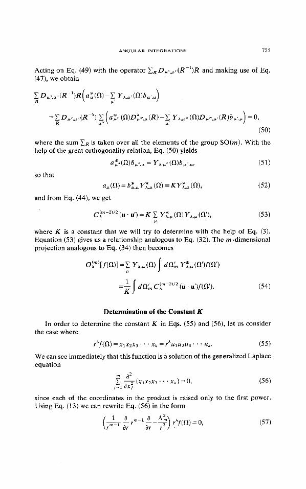
Acting on Eq. (49) with the operator 1, Dfi,:fir,(R-')R and making use of Eq. (47), we obtain
R Dfir',fi''(R-')R( (a) -1 f i r y A , f i ' (a)bfi',fi)
=c Dfi",fi"(R-') c ( a z " ' ( a > D ~ " ' , f i ( R ) - ~ YA,fifr' (a)Dfi"',fi'(R)bfi',fi) =o, R fi fi'
(50)
where the sum C R is taken over all the elements of the group SO(m). With the help of the great orthogonality relation, Eq. (50) yields
az"(a)8fi",fi = YA,fi" (a)bfi",fi,
(a) = b;,@ Y?,fi (a) = KY?,, (Q),
(5 1)
(52)
so that
and from Eq. (44), we get
(53) ( m - 2 ) / 2 CA (u * u') = K c y?,fi (a) y A , f i (a'), fi
where K is a constant that we will try to determine with the help of Eq. (3). Equation (53) gives us a relationship analogous to Eq. (32). The m -dimensional projection analogous to Eq. (34) then becomes
oj;")[f(a)l= YA,w (a) d n k y?,fi (a')f(n) fi
1 K
=- j dnk cj\m-2)'2 (u * u')f(W). (54)
Determination of the Constant K In order to determine the constant K in Eqs. (55) and (56), let us consider
the case where
r A f ( 0 ) = ~ 1 ~ 2 x 3 * * X A = rAu1u2u3 * uA. ( 5 5 )
We can see immediately that this function is a solution of the generalized Laplace equation
since each of the coordinates in the product is raised only to the first power. Using Eq. (13) we can rewrite Eq. (56) in the form
726 AVERY AND WEN
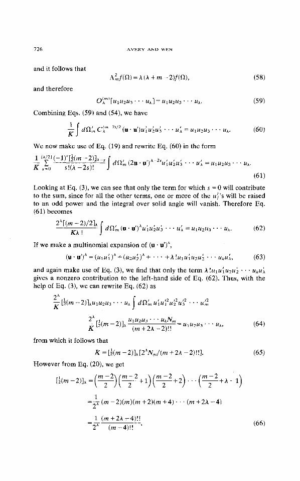
(61) Looking at Eq. (3), we can see that only the term for which s = 0 will contribute to the sum, since for all the other terms, one or more of the ui’s will be raised to an odd power and the integral over solid angle will vanish. Therefore Eq. (61) becomes
If we make a multinomial expansion of (u u’)”,
( U ‘ U ’ ) ” = ( U ~ U ~ ) ” + ( U Z U ; ) ” + “ * +h!UiU~U2U; ‘ * ‘ MAUL, (63)
and again make use of Eq. (3), we find that only the term A!uluiu2u; * uAul\ gives a nonzero contribution to the left-hand side of Eq. (62). Thus, with the help of Eq. (3), we can rewrite Eq. (62) as
12 r2 12 I2 2A [+(m -2)]AulU2u3 * - uA j u’ 1u1 u2 u3 * * - urn
from which it follows that
K=[$(m -2)]~[2”N,/(t?t +2A -2)!!].
However from Eq. (20), we get
m-2 m-2 m-2 [k(m - 211~ = ( T) ( T+ 1) ( T+ 2) . * (?+A - 1)
1 =-(m -2)(m)(m +2)(m +4) . (m t 2 A -4)
2”
2“ (m-4)!! ’ 1 (m+2A-4)!! =-
ANGULAR INTEGRATIONS 121
so that
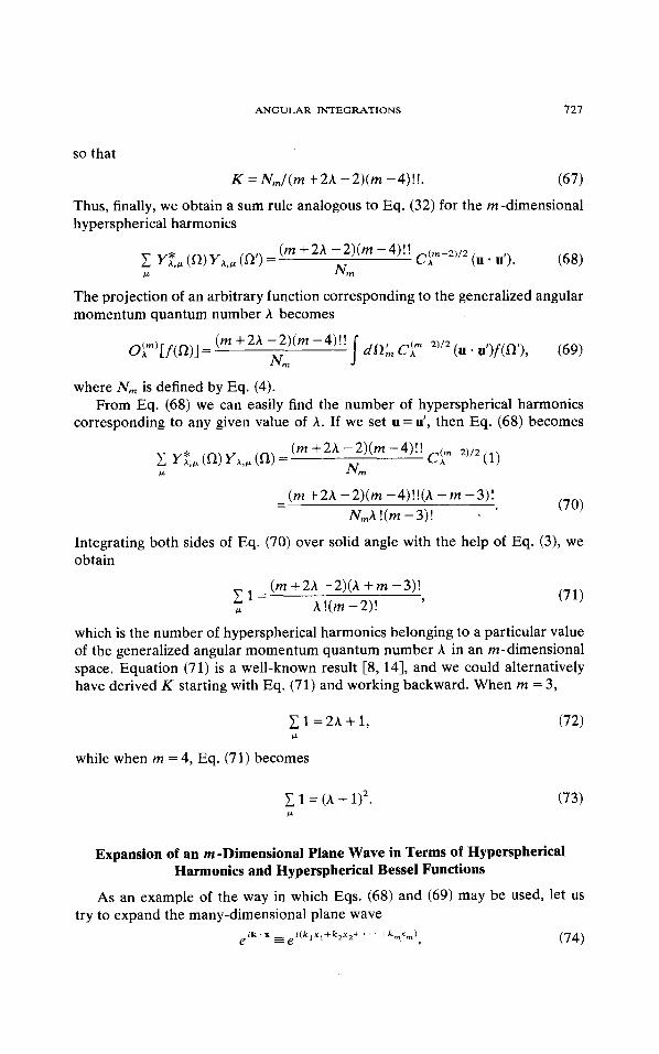
K = Nm/(m +2A - 2 ) ( m -4)!!. (67) Thus, finally, we obtain a sum rule analogous to Eq. (32) for the m-dimensional hyperspherical harmonics
The projection of an arbitrary function corresponding to the generalized angular momentum quantum number A becomes
d a l , Cim-2)'2 (u . u')f(Q'), (69) (m +2A -2)(m -4)!!
N m olm,""f(wl =
where Nm is defined by Eq. (4). From Eq. (68) we can easily find the number of hyperspherical harmonics
corresponding to any given value of A . If we set u = u', then Eq. (68) becomes
(70) - (m +2A -2)(m -4)!!(A + m -3)!
NmA!(m -3)! -
Integrating both sides of Eq. (70) over solid angle with the help of Eq. (3), we obtain
(m + 2A - 2)(A + m - 3)! E l = 9
& A!(m-2)!
which is the number of hyperspherical harmonics belonging to a particular value of the generalized angular momentum quantum number A in an m-dimensional space. Equation (71) is a well-known result [8, 141, and we could alternatively have derived K starting with Eq. (71) and working backward. When m = 3,
1 1 =2A +1, CL
while when m =4, Eq. (71) becomes
1 1 = (A + &
(73)
Expansion of an m -Dimensional Plane Wave in Terms of Hyperspherical Harmonics and Hyperspherical Bessel Functions
As an example of the way in which Eqs. (68) and (69) may be used, let us try to expand the many-dimensional plane wave
, (74) ik . x - i ( k , x , + k 2 x 2 + . . . + k m x , ) e = e
728 AVERY AND WEN
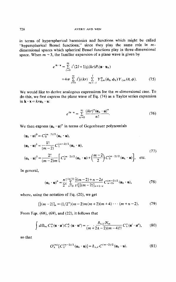
in terms of hyperspherical harmonics and functions which might be called "hyperspherical Bessel functions," since they play the same role in m - dimensional spaces which spherical Bessel functions play in three-dimensional space. When m = 3, the familiar expansion of a plane wave is given by
We would like to derive analogous expressions for the rn-dimensional case. To do this, we first express the plane wave of Eq. (74) as a Taylor series expansion in k . x = kruk * u:
We then express (uk . u)" in terms of Gegenbauer polynomials
( m - 2 ) / 2 (uk ' u)' = CO (uk u),
In general,
where, using the notation of Eq. (20), we get
[5(m - 2)ln = (1/2")(rn - 2)rn(rn + 2)(m + 4) - ( m + n - 2).
From Eqs. (68), (69), and (22), it follows that
c; (u' * u"), Sl\.l\"m I dam CP (u * U')CY, (u * u") = (rn +2h -2) (m -4)!!
ANGULAR INTEGRATIONS 729
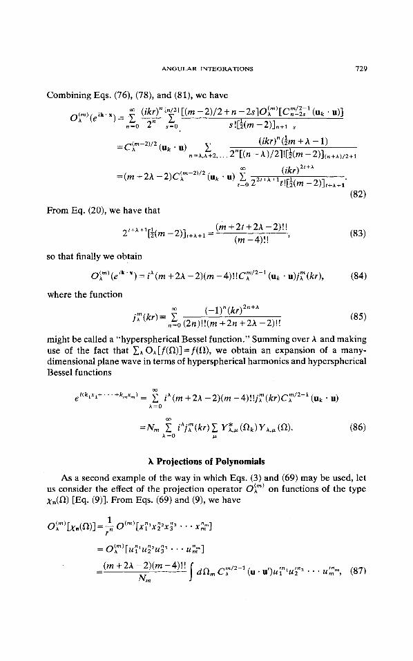
Combining Eqs. (76), (78), and (81)’ we have
From Eq. (20)’ we have that
(m +2t+2A -2)!! 2f+A+1[3(m -2)It+*+1 =
(m-4)!! ’ (83)
so that finally we obtain
O!im’(eik’”) = iA(m +2A -2)(m -4)!!C,”/2-’ (uk - u)j,”(kr), (84)
where the function 00 (- 1)” ( kr)2” +A
j , ” (kr )= c “=o (2n)!!(m +2n +2A -2)!!
might be called a “hyperspherical Bessel function.” Summing over A and making use of the fact that CAoA[f(fl)]=f(fl) , we obtain an expansion of a many- dimensional plane wave in terms of hyperspherical harmonics and hyperspherical Bessel functions
A Projections of Polynomials
As a second example of the way in which Eqs. (3) and (69) may be used, let us consider the effect of the projection operator Oim) on functions of the type ,y.(fl) [Eq. (913. From Eqs. (69) and (9), we have
730 AVERY AND WEN
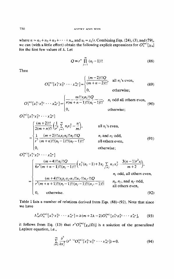
where n = nl + n2 + 123 + - * + n, and uj = x j / r . Combining Eqs. (24 ) , (3 ) , and (79 ) , we can (with a little effort) obtain the following explicit expressions for Oimm,[,yn] for the first few values of A. Let
m
Q = r " n ( n j - l ) ! ! j = l
Then
m ! !xjn j ! ! Q nj odd all others even, (90 ) r(m + n - I)!!(nj - I)!!' I o~""x;lx;z . . . x;m] =
otherwise;
1 (m +2)!!xjxj ,nj!!ni ,!!Q nj and nj, odd, r2 (m + n ) ! ! ( n i - l ) ! ! ( n j , - l ) ! ! ' all others even,
otherwise;
(m + 4 ) ! ! n j ! ! Q 6r3(m + n + l ) ! ! ( r Z j - l ) ! !
( x j ( n i - l ) + 3 x i C n j , x j , - 2 3(n;:i2xj), j'# j
ni odd, all others even,
0, otherwise. (92)
Table I lists a number of relations derived from Eqs. (88)-(92). Note that since we have
A~Ojr"'[x;'x~' * * * x",-]=A(m +2A - 2 ) 0 i m ' [ ~ ; ' ~ g ' * * * x ; ~ ] , ( 93 )
it follows from Eq. (13) that rAO~mm'[xn(fl)] is a solution of the generalized Laplace equation, i.e.,
ANGULAR INTEGRATIONS 731
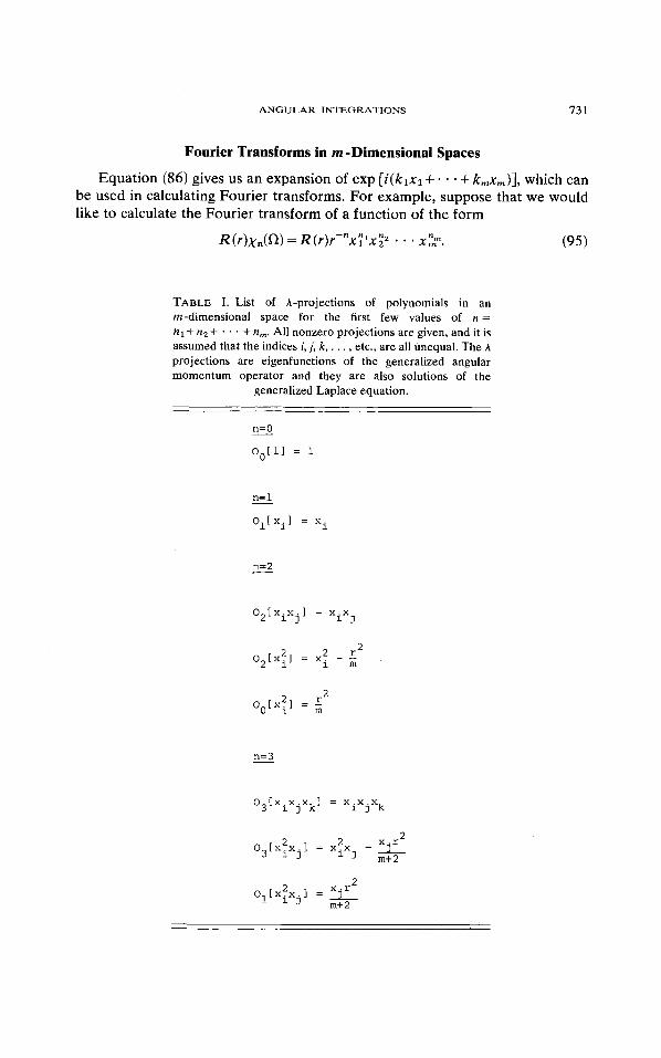
Fourier Transforms in m -Dimensional Spaces
Equation (86) gives us an expansion of exp [ i ( k l x l + * * + k,x,)], which can be used in calculating Fourier transforms. For example, suppose that we would like to calculate the Fourier transform of a function of the form
R(r)/y"(n) =R(r)r -"x; 'x;z * * * x",-. (95)
TABLE I. List of A-projections of polynomials in an m-dimensional space for the first few values of n = h l + n2 + . . . + n,. All nonzero projections are given, and it is assumed that the indices i, j , k, . . . , etc., are all unequal. The A projections are eigenfunctions of the generalized angular momentum operator and they are also solutions of the
generalized Laplace equation.
n=O -
00[11 = 1
n=l - Ol[Xi1 = xi
O2[XiXj1 = x i i x .
2 2 2 r 0 [x.] = x. - - 2 1 i m
0 [ x ] = L 2 2 O i m
0 [x x.x 1 = x . x .x 3 i l k l j k
2 0 [XZX.l = XiXj 2 - xjr
m+ 2 3 i j
2 2 Ol[XiXj1 = xjr m+ 2
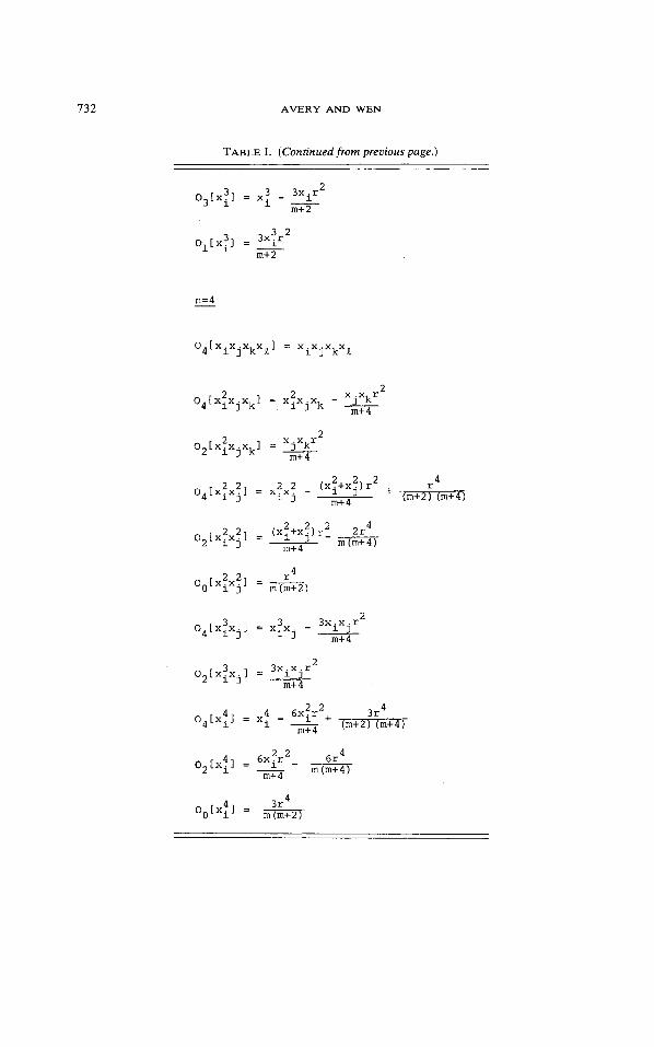
732 AVERY AND WEN
TABLE I. (Continued from previous page.)
3 2 ol[x;l = y
m+2
0 [x x.x x 1 = x x.x x 4 i j k L i j k R
2 3x .x .r 0 Lx3x.l = x3x. 4 i j 1 3 -*
02[xixj1 3 = 3xixjrL m+ 4
3r4 2 2 4 4 1 + (m+2) (m+4) 0 [x.] = x? - 6xir
m+ 4
4 4 6xir * - 6r m (m+4) O2[Xi1 = -
m+ 4
4 4 3r OO[Xi1 = - m (m+2)
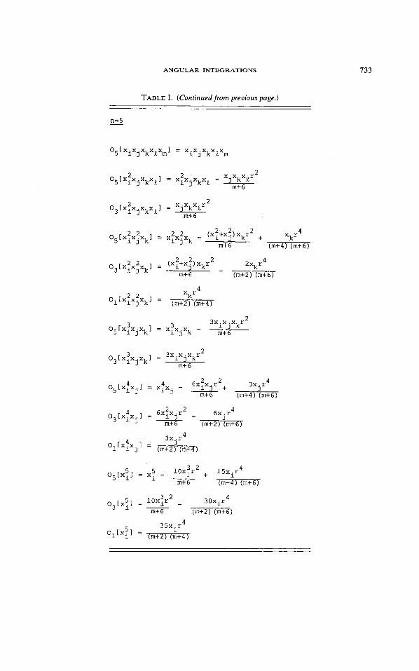
ANGULAR INTEGRATIONS 733
TABLE I. (Continued from previous page.)
n=5 -
0 [x x.x x x 1 = x.x.x x x 5 i j k k m i j k k m
2 2 0 [ x . x . ~ x 1 = x.x.x x - XjXkXLr2 5 l j k k i j k k m+ 6
0 [x 2 x x x 1 = xjxkxkr2
m+ 6 3 i j k i
4 2 2 xkr
(m+2) (m+4) 0 [x x.x 1 = 1 i j k
3x.x.x r2 3 3 i l k 0 [x x.x 1 = x.x.x - 5 i j k i l k n+ 6
2 0 [x 3 x.x 1 = 3xixjxkr m+ 6 3 i l k
4 4 3x . r4 0 5 [x i j x,] = x.x. 1 7 - - 6x1xjr2+ 3 (m+4) (m+6) m+ 6
4 6x?x. r2 6x.r4 o [ x x l = 1 7 - 1
m+ 6 (m+2) (m+6)
3x .r
3 i j
4 O,[XiXj1 4 = J
(m+2) (n+4)
5 5 10xir 3 2 + 15xir 4 O5[Xi1 = x. - __
m+ 6 (m+4) (m+6)
O3[Xi1 5 = - 10x:r2 - 30xir4 m+6 (m+2) (m+6)
734 AVERY AND WEN
Then from Eqs. (86), (68), and (69), we obtain
dxl dxz * * dx,e i ( k , x , + . . , + k m x m ) R(r)r-"x;Ix;Z . . . x-m I n
= 1 AA(k)k-n@,m'[k;'k;z * * * kkm], A = O
where
A A ( k ) = i A ( m +2A -2)(m -4)!! drr"-'jY(kr)R(r). (97) r The action of the projection operators Ol,"' on the product of kj's is given by Eqs. (88)-(92) and Table I with k's substituted for x's .
Subgroups of SO(m)
Let G be any subgroup of SO(m). For example, if the rn-dimensional space is the configuration space of a many-particle system, G might be the group of rotations of the system as a whole (i.e. the group whose irreducible representa- tions are characterized by eigenvalues of total orbital angular momentum). The hyperspherical harmonics corresponding to a given value of A form the basis of an irreducible representation Dk,CL, of SO(m). They also form the basis of a representation of G, but this representation will, in general, be reducible. Now let UCL,E be the unitary transformation matrix which reduces the representation of G based on the hyperspherical harmonics YA+. Then the functions
will be basis functions for irreducible representations of G. We would like to show that the functions ??IA,* obey a sum rule similar to Eq. (68). To show this, we note that the complex conjugate of Eq. (98) is
g:,S(a') = c yt,, (a') U L . * (99) C L I
Multiplying Eq. (98) by Eq. (99), summing over 8, and making use of the unitarity of the transformation matrix, we obtain
=c Y?,M (a') YA,@ (a)* CL
If we compare Eq. (100) with Eq. (68), we can see that the basis functions for the irreducible representations of G obey the sum rule
ANGULAR INTEGRATIONS 735
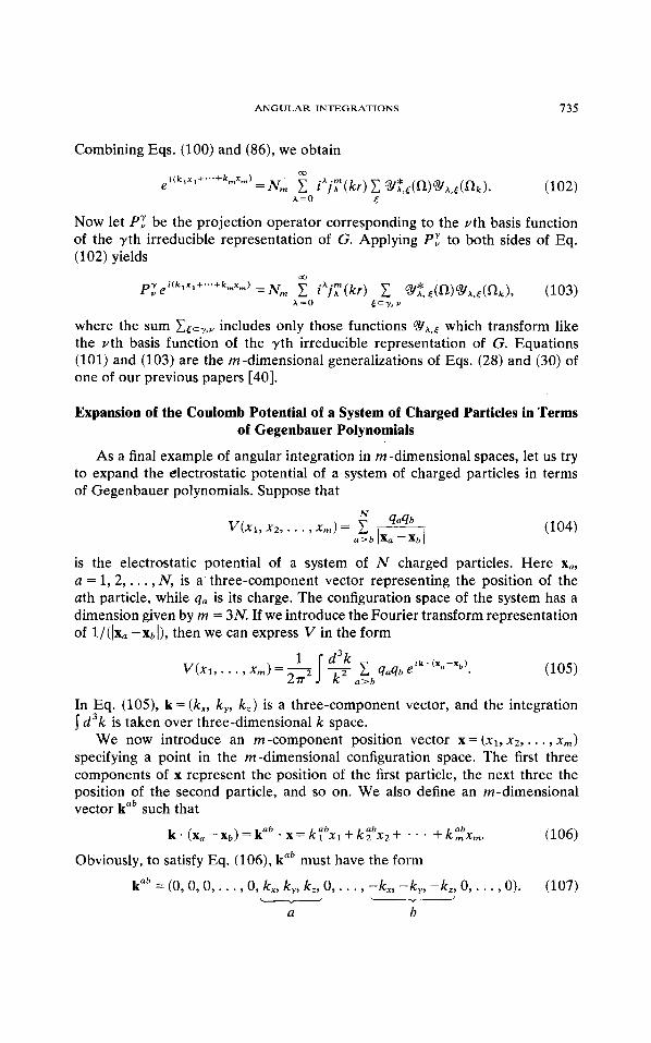
Combining Eqs. (100) and (86), we obtain m
(102) i(k,x,+~~~+k,x,) e =Nm C i A j Y ( k r ) C 9 ? , 5 ( f l ) % A , 5 ( f l k ) .
A = O 5
Now let P: be the projection operator corresponding to the vth basis function of the 7th irreducible representation of G. Applying P: to both sides of Eq. (1 02) yields
m
p ; ei (k ,x ,+~~~+k, , ,x , , , ) - -Nm C i A j T ( k r ) C ~ ? , c ( f l ) ~ ~ , ~ ( f l ~ ) , (103)
where the sum Ccc,.,v includes only those functions which transform like the vth basis function of the 7th irreducible representation of G. Equations (101) and (103) are the m-dimensional generalizations of Eqs. (28) and (30) of one of our previous papers [40].
A =O 5=r, Y
Expansion of the Coulomb Potential of a System of Charged Particles in Terms of Gegenbauer Polynomials
As a final example of angular integration in m-dimensional spaces, let us try to expand the electrostatic potential of a system of charged particles in terms of Gegenbauer polynomials. Suppose that
is the electrostatic potential of a system of N charged particles. Here x,, a = 1 , 2 , . . . , N, is a three-component vector representing the position of the uth particle, while qa is its charge. The configuration space of the system has a dimension given by m = 3N. If we introduce the Fourier transform representation of I/(lxa - x b l ) , then we can express v in the form
In Eq. (105), k = (k,, k,, k , ) is a three-component vector, and the integration
We now introduce an m-component position vector x = (XI, x 2 , . . . , x m > specifying a point in the m-dimensional configuration space. The first three components of x represent the position of the first particle, the next three the position of the second particle, and so on. We also define an m-dimensional vector kab such that
(106)
d 3 k is taken over three-dimensional k space.
ab k * (X, - X b ) = kab * x = k4'Xi + k;bX2 + * 9 * + k - x m .
Obviously, to satisfy Eq. (106), kab must have the form
kab = (0, 0, 0, . . . , 0, k,, k,, k,, 0,. . . , -k,, -k,, -kz , 0,. . . , 0). (107) - - U b
736 AVERY AND WEN
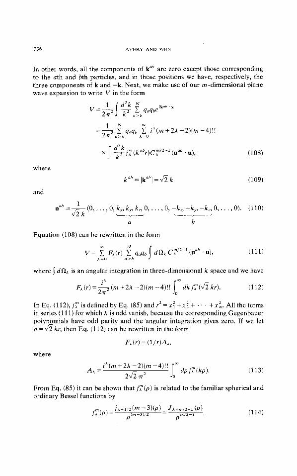
In other words, all the components of kab are zero except those corresponding to the ath and bth particles, and in those positions we have, respectively, the three components of k and -k. Next, we make use of our m-dimensional plane wave expansion to write V in the form
x $ jl:(kabr)C,”/2-’ (uab u),
and
Equation (108) can be rewritten in the form
where dRk is an angular integration in three-dimensional k space and we have
i“ 277
FA(r)=- (m +2A -2)(m -4)!!
2 In Eq. (112), j : is defined by Eq. (85) and r2 = x f + x i + * - +x,. All the terms in series (1 11) for which A is odd vanish, because the corresponding Gegenbauer polyn_omials have odd parity and the angular integration gives zero. If we let p = J2 kr, then Eq. (112) can be rewritten in the form
FA(r) = (1/r)&
where
From Eq. (85) it can be shown that j Y ( p ) is related to the familiar spherical and ordinary Bessel functions by
ANGULAR INTEGRATIONS 737
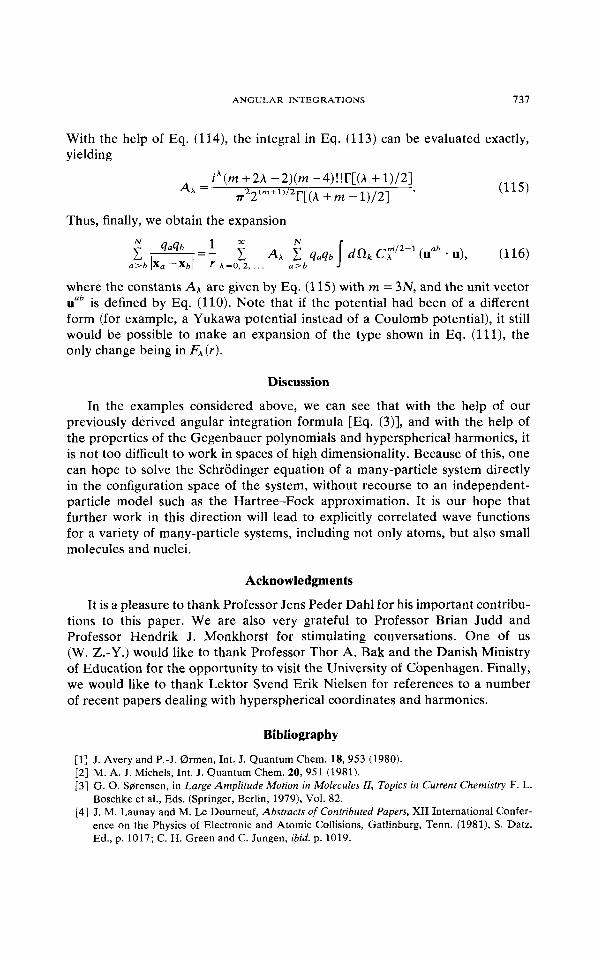
With the help of Eq. (114), the integral in Eq. (113) can be evaluated exactly, yielding
iA(m + 2 ~ -2)(m -4 ) ! ! r [ (~ +1)/2] T[(A + m - 1)/2] A, = T22(m+1)/2
Thus, finally, we obtain the expansion
where the constants A,+ are given by Eq. (115) with m = 3N, and the unit vector uab is defined by Eq. (110). Note that if the potential had been of a different form (for example, a Yukawa potential instead of a Coulomb potential), it still would be possible to make an expansion of the type shown in Eq. ( l l l ) , the only change being in FA ( r ) .
Discussion
In the examples considered above, we can see that with the help of our previously derived angular integration formula [Eq. (3)], and with the help of the properties of the Gegenbauer polynomials and hyperspherical harmonics, it is not too difficult to work in spaces of high dimensionality. Because of this, one can hope to solve the Schrodinger equation of a many-particle system directly in the configuration space of the system, without recourse to an independent- particle model such as the Hartree-Fock approximation. It is our hope that further work in this direction will lead to explicitly correlated wave functions for a variety of many-particle systems, including not only atoms, but also small molecules and nuclei.
Acknowledgments
It is a pleasure to thank Professor Jens Peder Dahl for his important contribu- tions to this paper. We are also very grateful to Professor Brian Judd and Professor Hendrik J. Monkhorst for stimulating conversations. One of us (W. Z.-Y.) would like to thank Professor Thor A. Bak and the Danish Ministry of Education for the opportunity to visit the University of Copenhagen. Finally, we would like to thank Lektor Svend Erik Nielsen for references to a number of recent papers dealing with hyperspherical coordinates and harmonics.
Bibliography
[l] J. Avery and P.-J. Qrmen, Int. J. Quantum Chem. 18, 953 (1980). [2] M. A. J. Michels, Int. J. Quantum Chem. 20, 951 (1981). [3] G. 0. Sprensen, in Large Amplitude Motion in Molecules 11, Topics in Current Chemistry F. L.
Boschke et al., Eds. (Springer, Berlin, 1979), Vol. 82. [4] J. M. Launay and M. Le Dourneuf, Abstracts of Contributed Papers, XI1 International Confer-
ence on the Physics of Electronic and Atomic Collisions, Gatlinburg, Tenn. (1981), s. Datz, Ed., p. 1017; C. H. Green and C. Jungen, ibid. p. 1019.
738 AVERY AND WEN
[5] B. R. Judd and E. E. Vogel, Phys. Rev. B 11,2427 (1975). [6] M. C. M. O’Brian, J. Phys. C 4,2524 (1971). [7] M. C. M. O’Brian, J. Phys. C 5, 2045 (1972). [8] M. J. M. Hill, Trans. Cambridge Philos. SOC. 13, 273 (1883). [9] J. D. Louck, J. Mol. Spectrosc. 4, 298 (1960).
[lo] T. Shibuya and C. E. Wulfrnan, Proc. R. SOC. London, Ser. A 286,376 (1965). [ll] B. R. Judd, Angular Momentum Theory for Diatomic Molecules (Academic, New York, 1975). [12] H. J. Monkhorst and B. Jeriorski, J. Chem. Phys. 71, 5268 (1979). [13] A. Erdelyi, W. Magnus, F. Oberhettinger, and F. G. Tricomi, Higher Transcendental Functions
(McGraw-Hill, New York, 1953). [141 N. J. Vilenkin, Special Functions and the Theory of Group Representations, Translations of
Mathematical Monographs, (American Mathematical Society, Providence, RI, 1968), Vol. 22. [15] F. T. Smith, Phys. Rev. 120, 1058 (1960). [16] F. T. Smith, J. Math. Phys. 3, 735 (1962). [17] R. C. Whitten and F. T. Smith, J. Math. Phys. 9, 103 (1968). [18] R. C. Whitten, J. Math. Phys. 10, 1631 (1969). [19] R. K. Bhaduri and Y. Nogarni, Phys. Rev. A 13, 1986 (1976). [20] H. Mayer, J. Phys. A 10, 1986 (1974). [21] C. D. Lin, Phys. Rev. A 14, 30 (1976). [22] C. D. Lin, Phys. Rev. A 14, 30 (1976). [23] J. H. Macek, Phys. Rev. 160, 170 (1967). [24] H. Klar and W. Schlecht, J. Phys. B 9, 1699 (1976). [25] C. W. Clark and C. H. Green, Phys. Rev. A 21, 1786 (1980). [26] G. 0. Morrell and D. L. Knirk, Theor. Chim. Acta 37, 345 (1975). [27] R. C. Whitten and J. S. Sims, Phys. Rev. A 9, 1586 (1974). [28] G. 0. Morrell, Doctoral thesis (Johns Hopkins University, Baltimore, 1979). [29] D. L. Knirk, J. Chem. Phys. 60, 66 (1974). [30] D. L. Knirk, J. Chem. Phys. 60, 760 (1974). [31] D. L. Knirk, Phys. Rev. Lett. 32, 651 (1974). [32] R. J. White and F. H. Stillinger Jr., J. Chem. Phys. 52, 5800 (1970). [33] W. G. Cooper and D. J. Kouri, J. Chern. Phys. 57,2487 (1972). [34] W. G. Cooper and D. J. Kouri, J. Math. Phys. 13, 809 (1972). [35] C. H. Greene, Phys. Rev. A 23,661 (1980). [36] M. Demiralp and E. Shuhubi, J. Math. Phys. 18, 777 (1977). [37] M. Demiralp, J. Chern. Phys. 72, 2828 (1980). [38] V. A. Fock, Izv. Akad. Nauk, SSSR Ser. Fiz. 18, 161 (1954). [39] L. M. Delves, Nucl. Phys. 9, 391 (1958-1959). [40] J. Avery and P.-J. armen, Int. J. Quantum Chem. 21, 515 (1982).
Received January 14, 1982 Accepted for publication March 23, 1982